Determination of pairing matrix elements from average single particle level densities

Abstract

A simple and efficient method to treat nuclear pairing correlations within a simple Hartree-Fock–plus-BCS description is proposed and discussed. It relies on the fact that the intensity of pairing correlations depends crucially on level densities around the Fermi surface ($\rho(e_{F})$) and that any fitting of nuclear energies as functions of the nucleon numbers is akin of a semi-classical average, smoothing out their quantal structure. A particular attention has been paid to two points generally ignored in previous similar approaches. One is a correction advocated by Möller and Nix [Nucl. Phys. A 536, 20 (1992)] taking into account the fact that the data included into the fit correspond to $\rho(e_{F})$ values systematically lower than average. The second is due to a systematic overestimation of the proton sp level density at the Fermi surface resulting from the local Slater approximation of the Coulomb terms in use in most microscopic descriptions. Our approach is validated by the agreement with data of corresponding calculated moments of inertia of well and rigidly deformed rare-earth nuclei, evaluated according to the Inglis-Belyaev ansatz with some crude Thouless-Valatin corrections. Indeed, the agreement which is found, is at least of the same quality as what results from a specific fit of the pairing intensities to these particular pieces of data. While this approach is currently limited to the very simple seniority force pairing treatment, it may serve as a starting point to define pairing residual interactions from averaged odd-even mass differences data, using merely average sp level densities associated to calculated canonical basis.

I Introduction

We aim at discussing a simple and phenomenologically successful approach to determine the intensity of a pairing residual interaction used in a two-steps self-consistent approach of low energy nuclear structure as currently performed and sketched below.

A self-consistent mean field is calculated upon using any particle-hole effective interaction (here the Skyrme parametrisation will be considered for the strong interaction part). This defines a single particle (sp) canonical basis from which pairing correlations are introduced either within a self-consistent Hartree-Fock (HF) approach (see the seminal paper [1]) or within a diagonalisation in a highly truncated particle-hole basis (the so-called HTDA as introduced in [2]).

In order to do so, one makes an appropriate choice of the residual interaction: seniority force (constant pairing matrix elements around the chemical potential), delta interaction possibly with a density dependence to enhance the surface effects [3], Gaussian in $r$-space or separable in $p$-space [4]. Here, as a first step, to demonstrate the validity and performance of the general approach we will consider the simple seniority force ansatz.

Bohr, Mottelson and Pines [5] have pointed out, in particular, two nuclear spectroscopic properties strongly contingent upon pairing correlations (odd-even mass differences $\delta E$ and moments of inertia $\mathcal{J}$ (MoI), i.e., in practice, the first 2⁺ energies in well and rigidly deformed nuclei). Both are a priori accessible to a theoretical description within the above defined self-consistent approaches.

In a previous paper [6], making two independent fits of these two properties in the rare earth region, it has been shown that one has obtained very similar values for the parameters of the seniority force matrix elements. This provides hints that: a) as expected, pairing correlations are indeed (all things being kept similar) the main factor to yield precise values of $\delta E$ as well as $\mathcal{J}$, and b) that such a simplified approach, also followed here, was suited globally to describe these properties.

However, in both approaches the quality of the agreement with data was locally (i.e. around a given nucleus) contingent upon a perfect reproduction of the ordering and fine distribution of the sp energies. But a fit corresponds in its very principle to a reproduction of some properties on the average. The above quoted success was obtained upon considering reasonably sized samples so one could conclude that on the average the regime of pairing correlations was correctly adjusted.

Taking stock of this remark, we have chosen here to perform an estimate of the pairing strengths using a tool a priori less sensitive to local sp spectrum deficiencies. The question we ask ourselves here is whether in doing so, we would obtain a reproduction of MoI at least as good as what has been obtained by a direct fit of these moments (see Ref. [6]).

In practice we used the so-called uniform gap method ([7], see also Ref. [8]) providing a value of the average matrix elements (around the Fermi energy) of the pairing residual interaction upon adopting an adequate smooth parametrisation of the neutron and proton pairing gaps $\Delta(N,Z)$.

Some special attention has been paid to two important points of a different nature.

The first issue is of a physical nature. Some analytical forms of the $\Delta(N,Z)$ function have been proposed by Jensen et al. [9] and Madland and Nix [10], but Möller and Nix [11] have pointed out a systematic bias of these approaches related with the lower than average character of the sp level density at equilibrium deformations. They proposed a phenomenological correction which we will adopt in this paper.

The second point concerns an approximation made in most self-consistent calculations (including most of ours) for the sake of numerical easiness. In previous studies (e.g. in Table II of [6]) one has noticed that the treatment of pairing correlations was significantly more successful for neutrons than it was for protons. It has been hinted that it was related to an approximate treatment of the non-local Fock term of the Coulomb mean field due to Slater [12]. As discussed in Sub-Section II.4, this approximation systematically overestimates the sp level density near the Fermi level [13, 14, 15]. A proper account of this spurious enhancement was thus in order and an appropriate correction to the proton sp level density has been implemented upon comparing the effect of the Coulomb exchange terms issued from approximate and exact calculations.

Calculations have been performed for a sample of $19$ lanthanide nuclei supplemented by three isotopes of Hafnium and one isotope of Tungsten (hereafter loosely refered to as rare earth nuclei) and 22 actinide nuclei. They are listed in Table 1. These nuclei are well ($\beta_{20}$ values in the $0.2-0.3$ range with usual notation) and rigidly deformed. The latter property is ascertained by a ratio of their first $2^{+}$ and $4^{+}$ levels $R_{42}\geq 3.290$ as displayed in Table 1 (energy data taken from the compilation of Ref. [16]).

Table 1: The ratio of the first $4^{+}$ over $2^{+}$ energy $R_{42}$, the estimated neutron $V_{n}$ and proton $V_{p}$ pairing matrix elements (in MeV), the calculated MoI (in $\hbar^{2}/\mbox{MeV}$), including a Thouless-Valatin corrective factor of $\alpha=1.32$, obtained with the SIII, SkM* and SLy4 parametrisations and the experimental MoI extracted from the first $2^{+}$ energy, $\mathcal{J}_{exp}$, for a nucleus with $Z$ protons and $N$ neutrons. Actinide nuclei removed from the MoI r.m.s analyses presented in Table 4 are marked with dashed lines.

Z	N	A	$R_{42}$	SIII			SkM*			SLy4			$\mathcal{J}_{exp}$
				$V_{n}$	$V_{p}$	$\mathcal{J}_{TV}$	$V_{n}$	$V_{p}$	$\mathcal{J}_{TV}$	$V_{n}$	$V_{p}$	$\mathcal{J}_{TV}$
62	94	156	3.290	0.1901	0.2529	37.742	0.1769	0.2450	39.438	0.2013	0.2537	38.221	39.531
62	96	158	3.301	0.1862	0.2517	38.068	0.1727	0.2440	42.063	0.1964	0.2527	37.148	41.209
62	98	160	3.292	0.1818	0.2510	40.765	0.1683	0.2435	40.693	0.1916	0.2518	39.215	42.373
64	96	160	3.302	0.1865	0.2454	36.537	0.1735	0.2383	39.943	0.1970	0.2467	35.192	39.860
64	98	162	3.302	0.1822	0.2442	40.663	0.1694	0.2377	38.840	0.1925	0.2453	38.258	41.899
64	100	164	3.295	0.1776	0.2430	40.657	0.1651	0.2370	38.136	0.1880	0.2445	42.849	40.944
64	102	166	3.297	0.1738	0.2422	42.775	0.1612	0.2366	39.549	0.1843	0.2437	37.230	42.857
66	96	162	3.294	0.1867	0.2389	35.283	0.1742	0.2308	38.742	0.1974	0.2393	35.302	37.193
66	98	164	3.301	0.1825	0.2379	39.453	0.1701	0.2302	38.577	0.1931	0.2381	39.004	40.876
66	100	166	3.310	0.1783	0.2373	38.850	0.1645	0.2294	38.936	0.1888	0.2372	43.868	39.171
66	102	168	3.313	0.1743	0.2367	40.901	0.1564	0.2290	42.649	0.1847	0.2359	38.845	40.021
68	100	168	3.309	0.1797	0.2318	36.297	0.1669	0.2224	37.682	0.1893	0.2319	41.603	37.592
68	102	170	3.310	0.1749	0.2307	39.076	0.1631	0.2217	39.339	0.1854	0.2302	37.400	38.173
68	104	172	3.314	0.1712	0.2296	35.341	0.1605	0.2209	39.610	0.1796	0.2287	36.688	38.961
70	100	170	3.293	0.1791	0.2261	35.754	0.1674	0.2167	38.655	0.1895	0.2266	40.594	35.606
70	102	172	3.305	0.1753	0.2246	37.865	0.1637	0.2154	41.260	0.1859	0.2244	37.624	38.099
70	104	174	3.310	0.1717	0.2227	35.636	0.1602	0.2135	43.698	0.1823	0.2221	37.465	39.231
70	106	176	3.310	0.1681	0.2215	34.882	0.1567	0.2120	42.205	0.1786	0.2202	38.821	36.525
70	108	178	3.310	0.1646	0.2204	37.397	0.1533	0.2109	42.128	0.1756	0.2185	38.506	35.714
72	106	178	3.291	0.1686	0.2164	31.988	0.1573	0.2108	33.572	0.1789	0.2188	33.180	32.196
72	108	180	3.307	0.1652	0.2154	33.615	0.1539	0.2097	31.557	0.1753	0.2175	31.464	32.146
72	110	182	3.295	0.1617	0.2144	31.436	0.1506	0.2089	31.185	0.1725	0.2165	31.184	30.678
74	108	182	3.291	0.1653	0.2112	30.384	0.1543	0.2061	27.708	0.1753	0.2141	27.755	29.968
90	144	234	3.291	0.1216	0.1744	57.708	0.1131	0.1671	65.546	0.1297	0.1715	74.584	60.545
92	140	232	3.291	0.1254	0.1632	63.879	0.1172	0.1628	-	0.1340	0.1678	76.273	63.061
92	142	234	3.296	0.1235	0.1698	-	0.1153	0.1630	-	0.1291	0.1677	82.008	68.969
92	144	236	3.304	0.1217	0.1700	63.052	0.1135	0.1634	-	0.1300	0.1678	84.126	66.307
92	146	238	3.303	0.1203	0.1701	59.663	0.1117	0.1639	-	0.1281	0.1682	71.416	66.791
92	148	240	3.347	0.1181	0.1704	-	0.1099	0.1642	-	0.1262	0.1691	63.613	66.667
94	142	236	3.304	0.1237	0.1654	-	0.1156	0.1599	71.615	0.1291	0.1593	-	67.219
94	144	238	3.312	0.1219	0.1654	67.935	0.1138	0.1601	70.205	0.1250	0.1645	-	68.081
94	146	240	3.309	0.1201	0.1656	65.827	0.1120	0.1602	73.433	0.1284	0.1647	71.278	70.054
94	148	242	3.307	0.1183	0.1703	61.921	0.1103	0.1606	-	0.1265	0.1650	66.699	67.355
94	150	244	3.391	0.1167	0.1663	63.423	0.1086	0.1609	64.584	0.1248	0.1654	73.284	67.873
94	152	246	3.308	0.1150	0.1669	-	0.1075	0.1612	59.134	0.1233	0.1656	59.224	64.240
96	146	242	3.252	0.1202	0.1622	-	0.1123	0.1565	-	0.1290	0.1611	-	71.208
96	148	244	3.314	0.1185	0.1626	66.225	0.1061	0.1566	-	0.1267	0.1610	70.430	69.837
96	150	246	3.313	0.1169	0.1630	65.332	0.1091	0.1569	68.096	0.1250	0.1612	-	70.008
96	152	248	3.313	0.1152	0.1635	-	0.1073	0.1571	64.122	0.1197	0.1614	65.674	69.124
98	150	248	3.318	0.1170	0.1597	63.764	0.1093	0.1532	71.893	0.1251	0.1592	-	72.237
98	152	250	3.321	0.1153	0.1599	-	0.1076	0.1534	68.774	0.1234	0.1578	67.810	70.223
98	154	252	3.319	0.1138	0.1640	-	0.1060	0.1537	62.400	0.1216	0.1579	61.026	65.617
100	154	254	3.319	0.1139	0.1560	-	0.1063	0.1499	64.823	0.1218	0.1546	62.273	66.679
100	156	256	3.317	0.1098	0.1560	-	0.1047	0.1502	59.527	0.1201	0.1545	61.250	62.344
102	150	252	3.310	0.1152	0.1520	67.468	0.1097	0.1469	-	0.1252	0.1521	-	64.655

The paper is organised as follows. The general fitting approach is presented in Section II. The extraction of averaged sp level density is performed à la Strutinsky [7] from our microscopic calculations for a sample of well and rigidly deformed nuclei. The uniform gap method is used to extract the matrix element of the pairing residual interaction upon using the Möller-Nix ansatz for average $\Delta(N,Z)$ values. The definition of effective average gaps to be fitted as well as the correction in the proton case for the approximation made on the Fock Coulomb terms are also discussed there. Some technical details are briefly presented in Section III. They include the choice of the sample of deformed nuclei in the two considered regions of heavy deformed nuclei (around rare-earth and actinide elements) and the specific choice made for the Strutinsky averaging of the sp level density. Our results obtained with three parametrisations of the Skyrme interaction, namely SIII [17], SkM* [18] and SLy4 [19], for the moments of inertia are presented in Section IV. Finally, Section V summarizes the main conclusions of our work.

II The approach

II.1 Overview of the approach

Assuming that we know the smooth behaviour of the average neutron and proton pairing gaps with $N$ and $Z$, we devise here an approach to get the corresponding smooth evolution of pairing matrix elements $V_{q}$ (where $q$ stands for the charge states) averaged over a given sp valence space being contained in the $[\lambda_{q}-\Omega,\lambda_{q}+\Omega]$ range where $\lambda_{q}$ is the Fermi energy to be defined later, while the above energy interval (spanning a $2\Omega$ energy range) characterizes the domain of sp states (of the canonical basis) active in the BCS treatment. In this work we will take $\Omega=6$ MeV.

From the exact sp level density $\rho(e)$ as a function (rigorously speaking distribution) of the energy $e$, we define a semi-classical sp level density function $\tilde{\rho}(e)$ obtained in practice by a Strutinsky averaging in $e$ [7]. We recall here the close connection of the Strutinsky energy averaging with a semi-classical averaging à la Wigner-Kirkwood (see Ref. [20]).

As stated in the introduction, we restrict ourselves in this work to constant pairing matrix elements $V_{q}$ for each charge state $q$ within an energy range of $2\Omega$ centered around averaged Fermi energies $\tilde{\lambda}_{q}$ defined below. Limiting the interval of sp states active in the BCS variational process makes the value of $V_{q}$ dependent on the value of $\Omega$, as well known. Here consistently we will take $\Omega=6$ MeV.

The matrix elements $V_{q}$ are determined in terms of the averaged sp level densities $\tilde{\rho}_{q}(e)$ and the average pairing gaps $\tilde{\Delta}_{q}$ through the following gap equation:

$$\frac{1}{V_{q}}=\int_{\tilde{\lambda}_{q}-\Omega}^{\tilde{\lambda}_{q}+\Omega}\frac{\tilde{\rho}_{q}(e)}{\sqrt{(e-\tilde{\lambda}_{q})^{2}+{\tilde{\Delta}}_{q}^{2}}}de.$$ (1)

The Fermi energies $\tilde{\lambda}_{q}$ are defined from the average density ${\tilde{\rho}}_{q}(e)$ for a total fermion number $N_{q}$ such that

$$N_{q}=\int_{-\infty}^{\tilde{\lambda}_{q}}\tilde{\rho}_{q}(e)de.$$ (2)

A frequently used approximation of the above gap equation consists in assuming that the variation of ${\tilde{\rho}}_{q}(e)$ is small enough within the $[\tilde{\lambda}_{q}-\Omega,\tilde{\lambda}_{q}+\Omega]$ sp energy interval so that one can replace it by a constant, namely its Fermi energy value ${\tilde{\rho}}_{q}(\lambda_{q})$. Upon performing the integral one then obtains a closed form formula for $V_{q}$ as

$$\frac{1}{V_{q}}=\frac{1}{2}{\tilde{\rho}}_{q}(\lambda_{q})sinh^{-1}\Big{(}\frac{\Omega}{{\tilde{\Delta}}}_{q}\Big{)}.$$ (3)

This approximation is shown to be indeed rather good as displayed in Figure 1 where we have plotted the difference in the pairing matrix elements obtained using equation (1) and (3) using an integration interval defined by $\Omega=6$ MeV. The difference in the proton pairing matrix elements between the two equations is mostly localized between $\pm 1$ keV while the largest difference for neutrons in absolute value is $4.3$ keV.

While we have shown en passant that the approximate equation (3) is a rather good approximation, we have however resorted to making a full integration using equation (1) for our calculations.

At the end of this process, we will then have for each charge state an average matrix element of the pairing residual interaction $V_{q}(N,Z)$ as a function of $N$ and $Z$.

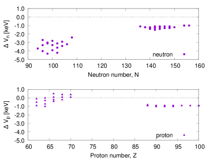
Figure 1: Difference in pairing matrix elements $\Delta v_{q}$ between values obtained using a full integration over the pairing window $\Omega$ and those obtained using the asinh function given in equation (3)

II.2 Determination of the average single-particle level density

The crucial part is then to determine the average level density for a given set of sp levels. We have computed the average level density using the equation [7, 21]

$$\tilde{\rho}_{q}(e)=\frac{1}{\gamma}\int_{-\infty}^{\infty}\rho(e^{\prime})f\Big{(}\frac{e^{\prime}-e}{\gamma}\Big{)}de^{\prime}.$$ (4)

The so-called curvature corrections (as discussed in Refs. [7, 21]) are taken care of by the $f(x)$ term defined as

$$f(x)=P(x)\>w(x)$$ (5)

where $P(x)$ is a polynomial of degree $2M$ in $x$ defined in terms of generalized Laguerre polynomials $L_{M}^{(\alpha)}$ of the form

$$P(x)=L_{M}^{1/2}(x^{2})=\sum_{n=0}^{M}a_{2n}\>x^{2n}.$$ (6)

with coefficients $a_{2n}$ given in Table 2 and $w(x)$ being a weightage of Gaussian type defined by

$$w(x)=\frac{1}{\sqrt{\pi}}e^{-x^{2}}.$$ (7)

M	$a_{0}$	$a_{2}$	$a_{4}$	$a_{6}$	$a_{8}$
0	1	–	–	–	–
1	3/2	-1	–	–	–
2	15/8	-5/2	1/2	–	–
3	35/16	-35/8	7/4	-1/6	–
4	945/384	-315/48	63/16	-9/12	1/24

Table 2: Five lowest generalized Laguerre polynomial coefficients entering equation (6).

The value of the smoothing width $\gamma$ appearing in equation (4) is crucial to define a correct energy window for the discrete sp levels to be considered in the integration of equation (4). This, as discussed e.g. in Refs. [7, 21], is generally defined by fulfilling the so-called plateau condition ensuring that the shell effect energy is almost constant as a function of $\gamma$.

In practice, we chose a value of $\gamma$ (in MeV) according to the total nucleon number $A$ as

$$\gamma=\beta\>\frac{41}{A^{1/3}}[MeV]$$ (8)

using the standard (see Ref. [22]) formula for the energy spacing between major oscillator shells. The specific value of the above constant $\beta$ and the polynomial order $2M$ in $x$ of $P(x)$ will be discussed in Sub-Section III.2.

II.3 Empirical vs effective-pairing gaps

The next crucial ingredient to the approach are the pairing gaps extracted from the data on $\delta E$, entering equation (1) or (3). At this point, it is important to differentiate between empirical pairing gaps as used e.g. in Refs. [9, 10] and those to be employed in any fitting approach such as ours. The latter are referred to as effective interaction pairing gaps in [11].

As discussed in [11], these effective gap values should take into account a bias due to the shell effects in the sp level density at equilibrium deformation making it systematically lower than its average value. Therefore the experimental pairing gaps should not be used as such to determine average pairing properties. Their values should be quenched since upon not doing that a fit of the residual interaction on them would lead to an overestimation of the pairing correlations in actual Hartree-Fock–plus–BCS (HF+BCS) calculations.

Herein, we use the effective-interaction average pairing gaps, phenomenologically determined in Ref. [11] to be:

$$\tilde{\Delta}_{q}=\frac{rB_{s}}{N_{q}^{1/3}}$$ (9)

where $B_{s}$ is set to $1$ and $r=4.8$ [11].

II.4 Effective pairing gaps in the proton case

In the case of protons, the above value of $r$ yields slightly too high BCS pairing gaps since the above formula corresponds supposedly to an exact treatment of the Coulomb interaction This is, however, not the case in most mean-field calculations. In order to avoid considering non-local mean fields, the Coulomb-exchange contribution is usually accounted for à la Slater, i.e. upon using the infinite nuclear matter Pauli correlation function [12]. As found long ago [13] and confirmed later [14, 15] the Slater approximation in use, systematically overestimates the sp level density near the Fermi level with respect to the corresponding exact treatment.

In order to correct for this systematic spurious trend modifying significantly the level density, we have proceeded as follows. We have considered for a given nucleus, two sp proton spectra obtained within the Skyrme HF+BCS framework, corresponding to an exact treatment and the Slater approximation of the Coulomb exchange terms. The exact calculation of the Coulomb energy matrix elements has been performed according to the method developed in Refs. [13] and [15]. This has yielded a corresponding ratio $R_{p}$ of the BCS gaps:

$$R_{p}=\frac{\Delta_{p}^{exact}}{\Delta_{p}^{Slater}}.$$ (10)

We take for granted the average effective gap of Ref. [11] (see equation (47)) with $r=4.8$ MeV as reproducing adequately effective average pairing matrix elements. For a given well and rigidly deformed nucleus and a given interaction, we perform calculations with the Slater approximation using the Möller-Nix value of $r$ and reasonable values (as defined below) of the average pairing matrix element for instance as (see the discussion of such a choice in Subsection III.1)

$$V_{q}^{0}=\frac{G_{q}}{11+N_{q}}\;\;\;\mbox{with}\;\forall_{q},\;G_{q}=19\;\mbox{MeV}.$$ (11)

It is well known that the sp spectra are almost unaffected by a variation of $V_{q}^{0}$ in quite a large range of values of around values such as those displayed above in eq. (11). This is demonstrated at least for the average sp level densities at the Fermi surface in Table 3. For two nuclei in their deformed ground states, ¹⁷⁶Yb and ²⁴⁰Pu, we have calculated $\tilde{\rho}_{q}(\lambda_{q})$ for three values of the intensity parameter $G_{q}=16,19,22$ MeV. They vary for both nuclei and for all values of $G_{q}$ no more than $0.1\%$. Therefore, the resulting values of the average pairing matrix elements $V_{q}^{1}$ contingent merely upon the sp spectra should seemingly not depend on the arbitrary chosen values of $V_{q}^{0}$. This is clearly so for the neutron matrix elements $V_{n}$ and not really the case for the proton matrix elements $V_{p}$, for reasons which will be discussed now.

It is not as simple as to perform calculations with these $V_{p}^{0}$ values taking exactly into account the Coulomb exchange calculations to get $\Delta_{p}^{exact}$ and then determine $R_{p}$ as defined in eq (10) to correct for the Möller-Nix parameter. It turns out that the value of $R_{p}$ depends on the chosen value of $V_{p}^{0}$ or in effect of the degree of pairing correlations as a monotonically increasing function. This could be expected since the more pairing correlations are present, the closer to a smoothed-out level density distribution one would get, making it more and more closer to the one present in infinite nuclear matter corresponding to the Slater approximation.

Let us assume, as it will be discussed in Appendix A, that we have at our disposal a universal formula relating $R_{p}$ with a quantity representing the degree of pairing correlations. Here, we consider the so-called pair condensation energy $E_{cond}^{p}$ for protons (the absolute value of the part of the HF+BCS energy which involves the abnormal density), given by

$$E_{cond}^{p}=\frac{\Delta_{p}^{2}}{V_{p}}.$$ (12)

Having at hand the function $R_{p}(E^{p}_{cond})$, we will proceed as follows.

We perform HF+BCS calculations with Coulomb à la Slater with the matrix elements $V_{p}^{0}$. We then obtain BCS pairing gaps $\Delta_{q}$ and in particular the proton gap $\Delta_{p}(V_{p}^{0})$ which combined with $V_{p}^{0}$ will provide us with $E_{cond}^{p}(V_{p}^{0})$ and the associated value $R_{p}^{0}$ of the gap ratio defined in eq. (10). It is clear that this ratio depends on the retained value for the initial proton pairing matrix element $V_{p}^{0}$. The necessity for an iterative determination of the correct ratio $R_{p}$ consistent with a corresponding matrix element $V_{p}$ should, in principle, be advocated.

However as it will be discussed at length in Appendix A, the convergence of this iterative process is indeed very fast. Furthermore, upon making some very limited preliminary studies, it is easy to determine a priori, for a given particle-hole interaction, an interval of initial values of $V_{p}^{0}$, previously dubbed as reasonable, such that the particular choices which are made for those, lead to insignificant corrections. It appears that the above mentioned choice of $G_{n}=G_{p}=19$ MeV is convenient in this respect. We therefore stick to the corresponding initial values of

$$r_{corr}=r\>R_{p}^{0}$$ (13)

without reiterative procedure. We get the final value $V_{p}^{1}$ of the proton average pairing matrix element as done in the first stage of this calculation for a given nucleus an a given interaction, using now the corrected value $r_{corr}$ of the Möller-Nix parameter for the estimation process.

As detailed in Appendix A, such a determination of the values of $R_{p}$ has been achieved for a restricted sample (with respect to the 45 nuclei listed in Table 1) of 19 nuclei in the case of SIII (17 nuclei for SLy4 and SkM*) Specifically, we have excluded nuclei exhibiting large large sp energy gaps leading to artifically low BCS pairing gap, in view of the well-known deficiency of the BCS approximation in such weak pairing regimes (see e.g. Ref [23]).

Table 3: The average Fermi level densities for neutrons and protons (in MeV^-1) are reported in columns 4 and 5, respectively, for the ¹⁷⁶Yb and ²⁴⁰Pu nuclei in the ground-state deformation characterized by its quadrupole moment $Q_{20}$ (in barns). Columns 6 and 7 give the corresponding fitted fitted values (in MeV) of the average matrix elements $V_{q}$ (with $M=2$, $\beta=1.2$). These values are generated from HF+BCS calculations using different $G_{q}$ values (equal for neutrons and protons) as reported in column 2.

Nucleus	$G_{q}$	$Q_{20}$	${\tilde{\rho}}_{n}(\lambda_{n})$	${\tilde{\rho}}_{p}(\lambda_{p})$	$V_{n}$	$V_{p}$
Yb-176	16	19.13	4.709	3.619	0.1681	0.2151
	19	18.73	4.710	3.622	0.1681	0.2215
	22	18.34	4.717	3.625	0.1680	0.2300
Pu-240	16	28.72	6.388	4.736	0.1201	0.1602
	19	28.26	6.386	4.735	0.1201	0.1656
	22	27.77	6.385	4.735	0.1201	0.1733

III Technical details

III.1 Generation of sp levels

We have performed HF+BCS calculations for the deformed nuclear ground-states using three Skyrme parametrizations, namely the SIII [17], SkM* [18] and SLy4 [19], for the strong interaction part of the particle-hole interaction.

The canonical basis is determined upon solving the HF equations resulting from the corresponding energy density functional of the one-body reduced density matrix including self-consistently the BCS occupation probabilities. The eigensolutions of the corresponding one-body Hamiltonian are obtained by projection of their eigenstates onto the eigenstates of an axially symmetrical harmonic oscillator, a choice consistent with the axial and intrinsic parity symmetries imposed onto our solutions.

The size of the deformation-dependent basis corresponds for spherical solutions to 17 major shells (i.e. with $N_{0}=16$ in the notation of [1]). The two parameters defining the size and the ellipsoidal deformation of the harmonic oscillator potential (i.e. $b$ and $q$ respectively in the notation of [1]) are optimised for each nucleus to yield the lowest equilibrium energy. Integrals involving the densities are performed using the Gauss-Hermite and Gauss-Laguerre approximate integration methods with 50 and 16 mesh points, respectively.

Pairing correlations are only considered in the isospin $T=1$ channel, which amounts in practice, for the considered nuclei far enough from the $N=Z$ line, to restrict to neutron-neutron and proton-proton pairing (thus for $|T_{z}|=1$). As already mentioned in Section I we define this residual pairing interaction $\widehat{v}_{res}$ from an average of its BCS matrix elements

$$V_{q}=\langle{i_{q}\bar{i_{q}}}|\widehat{v}_{res}\Big{(}|{j_{q}\bar{j_{q}}\rangle-|\bar{j}_{q}j_{q}}\rangle\Big{)}.$$ (14)

Now, we make a further phenomenological step considering as in Ref. [24] a specific dependence of $V_{q}$ on the neutron or proton numbers $N_{q}$ in the following form

$$V_{q}=\frac{G_{q}}{11+N_{q}},$$ (15)

and in what follows $G_{q}$ will be referred to as the pairing strength.

The validity of this parametrisation has been demonstrated by the quality of the description at the same time of odd-even mass differences and of moments of inertia obtained in Ref. [6]. A residual interaction is by definition dependent on the number of fermions (through the dependence of the mean field). Yet, it is worth noting that the above parametrisation does not necessarily represent only such a dependence but also, and may be primarily, in an average fashion, the corresponding dependence of the sp wavefunctions (e.g. through their size or compactness).

Thus our task here is to determine, as sketched in Section II, the two parameters $G_{n}$ and $G_{p}$ (and thus $V_{n}$ and $V_{p}$) for each of the 35 well and rigidly deformed nuclei in the rare earth and actinide regions (see Section IV for details). Our approach depends only on sp spectra (through the Fermi levels $\tilde{\lambda}_{q}$ and the value of the average sp level density at these energies $\tilde{\lambda}_{q}$). To get the sp spectra, we have considered pairing residual matrix elements defined by $G_{n}=G_{p}=19$ MeV, as already mentioned.

III.2 Choice of coefficients to determine average level density

Two important ingredients entering the equation  (1), apart from the choice of pairing gap $\tilde{\Delta}_{q}$ which has been addressed in Section II.3 are the order $M$ of the generalized Laguerre polynomial and the constant $\beta$.

To determine optimal values of $M$ and $\beta$, we performed fits of pairing matrix elements with $\Omega_{1}=\Omega_{2}=6$ MeV for two rare earth (¹⁶⁶Dy and ¹⁷⁶Yb) and two actinide (²⁴⁰U and ²⁵²No) nuclei. Figure 2 shows the variation of neutron (top panels) and proton (bottom panels) pairing matrix elements with $M$ and $\beta$ for these nuclei.

We searched for the values of $(M,\beta)$ pairs where a plateau in the average $V_{q}$ matrix elements is roughly achieved to ensure that they remain almost constant upon varying $\beta$. A value of $\beta<1$ is not sufficient to smooth the shell effect (see Figure 3) where some remnants shell effects are still apparent even for $\beta=1$. On the other hand, one must avoid too large $\beta$ values (e.g. such that $\beta\geq 1.6$) to avoid the dubious contribution of unbound sp states poorly approximated by their projection onto a truncated harmonic oscillator basis.

From the results displayed in Figure 2, we have taken as an optimal choice the following values of the smoothing parameters: $M=2$ and $\beta=1.2$.

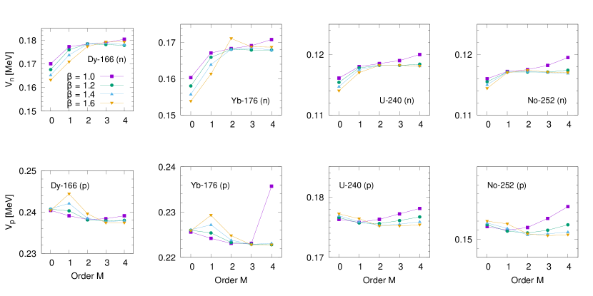
Figure 2: Variation of neutron (top panels) and proton (bottom panels) pairing matrix elements showing their evolution as a function of the order $M$ for different values of $\beta$.

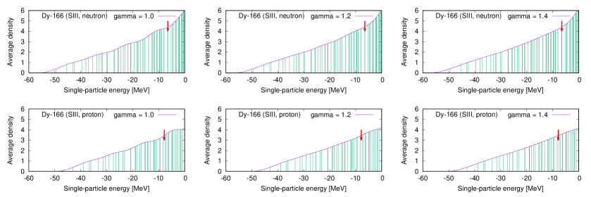
Figure 3: Average neutron (top panels) and proton (bottom panels) sp level densities (in MeV^-1) using equation (1) for the Dy-166 nucleus with $M=2$ and $\beta=1.0,1.2$ and $1.4$ as a function of sp energies. Red arrows indicated the location of the Fermi level.

IV Results

Using the approach discussed above, we calculated the MoI using the Inglis-Belyaev [25] formula with the estimated pairing strengths unique to each nucleus. To account approximately for the Thouless-Valatin selfconsistency correction (see Ref. [26]) the calculated MoI have been multiplied by a factor $1.32$, as suggested in Ref. [27] and shown in previous calculations (see e.g. Ref. [6]) to provide good estimates of this effect, for the three Skyrme parametrisations. The experimental MoI $\mathcal{J}_{exp}$ are determined from the energies of the first $2^{+}$ excited state in the pure rotor limit (these energies are taken from the compilation of Ref. [16] and tabulated in Table 1).

Prior to comparing our calculated MoI with experimental data, we further eliminate some actinide nuclei which exhibit deficiencies in the sp levels spectra. These nuclei marked with dashed lines in Table 1, all of which are in the heavy nuclei region, shows large energy gap located at incorrect nucleon number. In such nuclei, comparing the calculated MoI with experimental data would not be meaningful as the observed deviation is not due to the estimation procedure proposed herein, but rather due to the underlying mean-field solution, providing locally an inadequate sp level distribution at the Fermi surface.

Indeed, the proposed method which relies on an semi-classical averaging is blind to the existence of a large sp energy gap. As examples to this point, we refer to the ²⁴⁶Pu and ²⁴⁸Cm ($N=152$) isotones listed in Table 1. In Ref. [28] it was reported that an incorrect energy gap was found at $N=152$ with the SIII parametrisation. This deficiency is not propagated to the estimated $V_{n}$ as can be clearly seen when comparing the estimated $V_{n}$ with its neighbouring nuclei.

For comparison between our calculated values with experimental MoI, we look at the root-mean-square (r.m.s) deviation $\chi_{\mathcal{J}}$ such that

$$\chi_{\mathcal{J}}=\sqrt{\frac{\sum_{i}^{N}(\mathcal{J}_{TV}^{i}-\mathcal{J}_{exp}^{i})^{2}}{N}}$$ (16)

where $N$ is the total number of sample nuclei. The r.m.s deviation have been analysed for 23 nuclei around rare-earth region with all three Skyrme parametrizations and 12 (13) actinide nuclei with SIII and SLy4 (SkM*) separately. The $\chi_{\mathcal{J}}$ are tabulated in the top part of Table 4.

We found that the $\chi_{\mathcal{J}}$ values ranges from $1.7$ to $3.0$ $\hbar^{2}/\mbox{MeV}$ in the rare-earth region and from $3.4$ to $4.6$ $\hbar^{2}/\mbox{MeV}$ in the actinide region. It is interesting to note here that the value of $\chi_{\mathcal{J}}\sim 1.77\>\hbar^{2}/\mbox{MeV}$ for rare earth nuclei only is indeed very close to the r.m.s deviation ($1.75\>\hbar^{2}/\mbox{MeV}$) obtained from average pairing strengths fitted to experimental MoI in Ref. [6].

In comparing the $\chi_{\mathcal{J}}$ values, it appears that the agreement with data is less spectacular in the actinide region as compared to the rare-earth region. However, comparison of r.m.s deviation based on $\chi_{\mathcal{J}}$ defined in equation (16) is not suitable since the number $A$ of nucleons are starkly different affecting thus the values of MoI through their $A^{5/3}$ dependence. To remove the $A$ dependence, we compare instead the weighted r.m.s deviation defined as

$$\chi_{\mathcal{J}}^{A}=\sqrt{\frac{\sum_{i}^{N}\Big{(}\frac{\mathcal{J}_{TV}^{i}-\mathcal{J}_{exp}^{i}}{A^{5/3}_{i}}\Big{)}^{2}}{N}}$$ (17)

$$\chi_{\mathcal{J}}^{exp}=\sqrt{\frac{\sum_{i}^{N}\Big{(}\frac{\mathcal{J}_{TV}^{i}-\mathcal{J}_{exp}^{i}}{\mathcal{J}_{exp}^{i}}\Big{)}^{2}}{N}}.$$ (18)

In doing so, we see that the agreement with experimental MoI are indeed better for actinides than rare-earth region for the SkM* and SLy4 parametrisations (see Table 4).

Finally, we show that these values of the weighted r.m.s deviation provides a way to estimate the uncertainty in the calculated MoI uniquely for each nucleus. We define two uncertainty ranges for $\mathcal{J}$ associated to a given nucleus displayed in Table 5 as $\Delta_{\mathcal{J}}^{A}$ (resp. $\Delta_{\mathcal{J}}^{exp}$) by multiplying $\chi_{\mathcal{J}}^{A}$ (resp. $\chi_{\mathcal{J}}^{exp}$ ) by $A^{5/3}$ (resp. by $J_{TV}$).

Table 4: Weighted root-mean-square deviations $\chi_{\mathcal{J}}$ (in units of $\hbar^{2}/\mbox{MeV}$), $10^{4}\>\chi_{\mathcal{J}}^{A}$ (in units of $\hbar^{2}/\mbox{MeV}$) and $10^{2}\>\chi_{\mathcal{J}}^{exp}$ as defined in equations (16), (17) and (18 between calculated and experimentally defined MoI obtained with the three Skryme parametrisations.

		SIII	SkM*	SLy4
$\chi_{\mathcal{J}}$	Rare earth	1.769	2.706	2.940
	Actinide	4.582	3.394	3.498
$\chi_{\mathcal{J}}^{A}$	Rare earth	3.515	5.080	5.883
	Actinide	4.844	3.588	3.621
$\chi_{\mathcal{J}}^{exp}$	Rare earth	4.548	7.230	7.551
	Actinide	6.671	5.168	5.248

Table 5: Uncertainty ranges for the moment of inertia of some nuclei $\Delta_{J}^{A}$ and $\Delta_{J}^{exp}$ as defined in the text.

Z	N	$\mathcal{J}_{TV}$	$\mathcal{J}_{exp}$	$\Delta^{A}_{\mathcal{J}}$	$\Delta^{exp}_{\mathcal{J}}$
62	98	40.765	42.373	1.658	1.854
68	100	36.297	37.592	1.798	1.651
72	106	31.988	32.196	1.980	1.455
92	140	63.879	63.061	4.243	4.261
94	150	63.423	67.873	4.615	4.231
102	150	67.468	64.655	4.870	4.501

V Conclusion

In this paper, we have proposed and discussed a simple and efficient method to treat pairing correlations within a microscopic (non-relativistic) description of the structure of atomic nuclei. It takes stock on the fact that the intensity of pairing correlations depends crucially on level densities around the Fermi surface. It is suited to approaches where one has a good knowledge of the particle-hole interaction (e.g. of the usual Skyrme type) yielding (possibly in a self-consistent manner) the normal density matrix (and its canonical basis). Then one searches for a relevant approach to the abnormal density matrix, typically in a HF+BCS framework.

At present, it is limited to a very simple ansatz, namely using constant pairing matrix elements for sp states located in the vicinity of the Fermi surface, dubbed as the seniority force pairing treatment. Moreover, it is only operative a priori, so far, to describe the ground states of well and rigidly deformed nuclei. As a result, it yields, in a well-defined fashion, the pairing average matrix elements suited for a given nuclear ground state and a given particle-hole interaction. It is furthermore important to recall that, by no means it gives any direct access to a residual interaction since its output includes some average information on the wavefunctions of the states around the Fermi surface, particularly their spatial extensions.

For limited that it is now, it may serve, however, as a basis to determine the ingredients of a more elaborate pairing treatment, i.e. defining univocally a residual pairing interaction (contingent now merely on the choice of the particle – hole interaction) and not some average of its matrix elements. This would allow to build up a BCS treatment which can be used more safely on two counts: for all nuclei and away from their equilibrium deformation. On the one hand, it would include explicitely (and not in the average) information on the structure of the relevant sp wavefunctions. And defining an effective residual Hamiltonian, it could be used in a natural fashion away from the limited region where it has made sense to have it fitted with some piece of data, on another hand. The study of this necessary extension is currently under completion and will be presented in a forthcoming publication. To reach that goal it was therefore necessary to assess, first, the quality of the approach discussed here, for what it has been specifically tailored.

To determine the relevant pairing matrix elements, we used smoothly varying (with nucleon numbers) gaps as in Refs. [9, 10] corrected according to the prescription of Ref. [11]. Experimental odd-even mass difference $\delta E$ are the raw data from where these gaps are extracted. Such energies depend of course on the shell structure which is generally well reproduced by state of the art microscopic calculations, yet allowing in some well localised regions to generate some misplacement or bad rendering of sp gap intensities in some low sp level density regions. This is why the information from existing fits of experimental data in terms of smoothly varying (with respect to the nucleon numbers) has not been directly compared with what results from quantal calculations but with their underlying semi-classical content, determined in an approximate fashion. The mere ingredient of the latter relevant to pairing properties within our pairing model is the average sp level density at the Fermi surface and the nucleon numbers of the considered nucleus.

In doing so two important features, absent so far in fits of the pairing intensity, to the best of our knowledge, have been carefully taken into account. One is the correction advocated by Möller and Nix [11] due to the unescapable selection of data corresponding to sp level densities systematically lower than average. The second is due to a systematic overestimation of the proton sp level density at the Fermi surface resulting from the local Slater approximation of the Coulomb exchange contribution to the total energy [13, 14, 15].

The test of our method has consisted in using the so-determined average pairing matrix elements (with three different Skyrme force pararetrisations) to compare within an Inglis Belyaev approach (plus some approximate Thouless-Valatin correction) MoI of about forty well and rigidly deformed rare-earth and actinide nuclei, with what is deduced from the experimental energies of their first $2^{+}$ levels. The good quality of the theoretical estimate of these experimental MoI has been assessed to be about the same as what had been obtained within the same Hartree-Fock plus seniority BCS approach, in a particular case (for rare earth nuclei and using the Skyrme SIII parametrisation) by a direct fit of these MoI.

This gives confidence on the relevance of what is proposed here and allows to take stock on it to tackle our more ambitious attempt to define pairing residual interactions from averaged $\delta E$ data, using merely average sp level densities at the Fermi surface of the calculated canonical basis .

Appendix A Reduction factor for the Moller-Nix parameter in the case of protons

We performed both exact Coulomb and Slater approximation calculations for a series of nuclei using the pairing matrix elements listed in Table 6. The obtained ratio $R_{p}$ of the BCS proton gaps from all three Skyrme parametrisations considered herein, are then plotted in Figure 4 as a function of proton condensation energy $E_{cond}^{p}$.

The ratio $R_{p}$ increases, albeit rather minimally, with $E_{cond}^{p}$ defined in equation (12). A fit of the data to a linear equation yields

$$R_{p}=0.0181\>E_{cond}^{p}+0.781.$$ (19)

This equation allows for an estimation of the reduction factor to the Möller-Nix parameter for any Skyrme parametrisation and at a given initial pairing matrix element $V_{p}^{0}$. Multiplying the initial Möller-Nix parameter $r=4.8$ with the reduction factor, one then obtains the proton pairing gap to be utilized in the estimation of pairing matrix element via equation (1).

Let us discuss finally the influence of the choice of the initial pairing matrix element $V_{p}^{0}$ on the retained value for the gap ratio and consequently on the renormalization of the Möller-Nix proton gap values to be used in the fit (see SubSection II.4). Upon calculating the ground state deformation solutions of our selected nuclei within the HF+BCS approach (using the seniority force model) we get proton pairing condensation energies. They are, as already noted, dependent upon the choice of the average pairing matrix elements in use in these calculations. From them, using equation 13 we should define new values of the proton gaps from which using the uniform gap method and the sp spectra, we could generate new proton pairing matrix elements $V^{1}_{p}$. And we could iterate this process to get a convergence of the pairing matrix elements.

The question now is how much change from $V_{p}^{0}$ could we expect for these new matrix elements $V^{1}_{p}$. To estimate that, we assume that we have chosen reasonable values of the original $V_{p}^{0}$, i.e. quantified, for instance, by a deviation of the resulting $E_{cond}$ from the value obtained through a converged solution of this iterative process by no more than $\pm\>20\%$. We see from Figure 4 that such an interval for $E_{cond}$ corresponds to an interval for $R_{p}$ (and thus on the proton gaps used in the fit) of $\sim\pm\>2\%$. From the approximation (shown to be rather good, see Figure 1) of equation 3 concerning the relation between $V_{p}$ and $\Delta_{p}$, we get readily

$$\frac{\delta V_{p}}{V_{p}}=\frac{x}{ln(\sqrt{x+\sqrt{x^{2}+1}})}\frac{1}{\sqrt{x^{2}+1}}\frac{\delta\Delta_{p}}{\Delta_{p}}$$ (20)

with $x=\frac{\Omega}{\Delta_{p}}$. Using the following values $\Omega=6$ MeV and $\Delta_{p}=1$ MeV, one obtains an uncertainty on $V_{p}$ within the $\pm\>0.8\%$ range.

A specific convergence study has been performed for the two deformed nuclei considered in Table 3 (¹⁷⁶Yb and ²⁴⁰Pu) for the three values of the proton pairing intensity parameter $G_{p}=16,19,22$ MeV. One sees on Table 7 that the value of the proton matrix element $V^{0}_{p}$ is converged at the keV level at the second or third iteration. Similarly, the mass quadrupole moment $Q_{20}$ is converged at the fm² level already at the third iteration, even sometimes at the second. The other lesson comparing the starting value of $V^{0}_{p}$ and the converged one, is that one may hint that a reasonable range for $V^{0}_{p}$ values would lie in between $G_{p}=16$ and $G_{p}=19$ MeV. This constitutes a very simple preliminary study, for any given specific particle-hole interaction, allowing to define a priori for a global study some value of $V^{0}_{p}$ close to a level of about $1\%$ to what an iterative process would produce.

In view of the rough nature inherent to the averaging character of the relation between $E_{cond}$ and $R_{p}$ we deem that the iterative process sketched above presents no solid practical justification to this paper which aims to illustrate a method for determination of pairing strengths with limited dependence on experimental data.

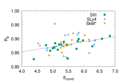
Figure 4: Ratio of the proton BCS gap between exact Coulomb and Slater approximation calculations $R_{p}$ as a function of the proton pairing condensation energy $E_{cond}$. All energies are given in MeV.

Table 6: The ratio $R_{p}$ of BCS proton pairing gap between Slater approximation $\Delta_{p}^{Slater}$ and exact Coulomb exchange $\Delta_{p}^{exact}$ calculations using the initial neutron and proton pairing matrix elements listed in column 4 and 5 respectively. The proton condensation energy defined in equation (12) are given in column 9.

	$Z$	$N$	$A$	$V_{n}^{0}$	$V_{p}^{0}$	$\Delta_{p}^{Slater}$	$\Delta_{p}^{exact}$	$R_{p}$	$E_{cond}^{p}$
SIII	62	94	156	0.1902	0.2686	1.0449	1.1884	0.879	5.2579
	62	96	158	0.1855	0.2682	0.9930	1.1319	0.877	4.7770
	64	96	160	0.1862	0.2600	1.0430	1.1894	0.877	5.4411
	66	98	164	0.1824	0.2520	1.0326	1.1612	0.889	5.3512
	66	100	166	0.1784	0.2515	1.0061	1.1436	0.880	5.1995
	66	102	168	0.1742	0.2511	0.9788	1.1254	0.870	5.0449
	68	104	172	0.1712	0.2433	0.9818	1.1108	0.884	5.0721
	70	104	174	0.1717	0.2363	0.9235	1.0772	0.857	4.9115
	70	106	176	0.1681	0.2358	0.8414	1.0169	0.827	4.3853
	72	106	178	0.1625	0.2291	0.9270	1.0700	0.866	4.9968
	74	108	182	0.1652	0.2227	0.9229	1.0715	0.861	5.1554
	92	142	234	0.1235	0.1765	0.9011	1.0114	0.891	5.7972
	92	148	240	0.1182	0.1756	0.9965	1.0954	0.910	6.8322
	94	148	242	0.1183	0.1720	0.8597	0.9952	0.864	5.7574
	94	150	244	0.1167	0.1718	0.9058	1.0375	0.873	6.2669
	96	148	244	0.1185	0.1686	0.7969	0.9611	0.829	5.4776
	98	154	252	0.1138	0.1646	0.9361	1.0406	0.900	6.5775
	100	154	254	0.1139	0.1615	0.8723	0.9700	0.899	5.8271
	100	156	256	0.1124	0.1612	0.8765	0.9806	0.894	5.9661
SLy4	62	94	156	0.2013	0.2688	1.2149	1.1111	0.915	5.4913
	62	96	158	0.1964	0.2678	1.2015	1.0971	0.913	5.3897
	64	96	160	0.1970	0.2603	1.2320	1.1356	0.922	5.8315
	66	98	164	0.1931	0.2523	1.1568	1.0111	0.874	5.3031
	66	100	166	0.1889	0.2516	1.1287	0.9786	0.867	5.0636
	66	102	168	0.1847	0.2507	1.0978	0.9427	0.859	4.8064
	68	104	172	0.1815	0.2432	1.0554	0.9247	0.876	4.5793
	72	106	178	0.1789	0.2300	1.1540	1.0573	0.916	5.7891
	74	108	182	0.1753	0.2237	1.1912	1.0646	0.894	6.3422
	92	148	240	0.1263	0.1742	1.0504	0.9242	0.880	6.3322
	94	146	240	0.1283	0.1717	0.9364	0.8173	0.873	5.1070
	94	148	242	0.1265	0.1712	0.9784	0.8606	0.880	5.5929
	94	150	244	0.1248	0.1707	1.0267	0.9148	0.891	6.1745
	96	148	244	0.1267	0.1681	0.8995	0.7800	0.867	4.8136
	98	154	252	0.1216	0.1637	0.9353	0.7838	0.838	5.3446
	100	154	254	0.1217	0.1609	0.9020	0.8601	0.954	5.0579
	100	156	256	0.1201	0.1603	0.9253	0.8174	0.883	5.3397
SkM*	62	94	156	0.1770	0.2574	1.2016	1.0758	0.895	5.6088
	62	96	158	0.1726	0.2570	1.1636	1.0319	0.887	5.2677
	64	96	160	0.1735	0.2493	1.2251	1.1169	0.912	6.0193
	66	98	164	0.1701	0.2414	1.1526	1.0119	0.878	5.5037
	66	100	166	0.1661	0.2409	1.1356	0.9898	0.872	5.3521
	66	102	168	0.1623	0.2405	1.1239	0.9740	0.867	5.2519
	68	104	172	0.1594	0.2331	1.0271	0.9068	0.883	4.5248
	72	106	178	0.1572	0.2199	1.1150	1.0251	0.919	5.6524
	74	108	182	0.1543	0.2138	1.1472	1.0296	0.897	6.1558
	92	148	240	0.1100	0.1675	1.0164	0.8614	0.848	6.1661
	94	146	240	0.1120	0.1644	0.9456	0.8330	0.881	5.4395
	94	148	242	0.1103	0.1642	0.9824	0.8719	0.888	5.8792
	94	150	244	0.1086	0.1639	1.0222	0.9149	0.895	6.3749
	96	148	244	0.1106	0.1609	0.9179	0.8042	0.876	5.2362
	98	154	252	0.1060	0.1570	0.9236	0.7692	0.833	5.4339
	100	154	254	0.1063	0.1539	0.8662	0.7278	0.840	4.8742
	100	156	256	0.1047	0.1537	0.9012	0.7656	0.850	5.2850

Table 7: Estimated proton pairing matrix elements $V_{p}$ (in MeV) at the ground-state quadrupole moments $Q_{20}$ (in barns) obtained for ¹⁷⁶Yb and ²⁴⁰Pu at corresponding iteration number with different starting initial pairing strength $G_{p}^{0}=16,19,22$ MeV. The estimated $V_{p}$ of the preceding iteration are used as initial values for subsequent HF+BCS calculations.

Nucleus	Iteration	$G_{p}^{0}=16$ MeV		$G_{p}^{0}=19$ MeV		$G_{p}^{0}=22$ MeV
		$Q_{20}$	$V_{p}$	$Q_{20}$	$V_{p}$	$Q_{20}$	$V_{p}$
Yb-176	1	19.13	0.2151	18.73	0.2215	18.35	0.2300
	2	18.89	0.2179	18.80	0.2189	18.74	0.2206
	3	18.88	0.2183	18.85	0.2185	18.83	0.2188
	4	18.86	0.2184	18.86	0.2185	18.85	0.2185
	5	18.86	0.2185	18.86	0.2185	18.86	0.2185
Pu-240	1	28.72	0.1602	28.26	0.1656	27.77	0.1733
	2	28.35	0.1614	28.34	0.1624	28.32	0.1639
	3	28.35	0.1615	28.35	0.1617	28.35	0.1620
	4	28.35	0.1616	28.31	0.1617	28.35	0.1616
	5	28.35	0.1616	28.35	0.1616	28.35	0.1616

References

- Flocard et al. [1973] H. Flocard, P. Quentin, A. Kerman, and D. Vautherin, Nucl. Phys. A 203, 433 (1973).
- Pillet et al. [2002] N. Pillet, P. Quentin, and J. Libert, Nucl. Phys. A 697, 141 (2002).
- Bochnacki et al. [1967] Z. Bochnacki, I. Holban, and I. Mikhailov, Nucl. Phys. A 97, 33 (1967).
- Tian et al. [2009] Y. Tian, Z. Ma, and P. Ring, Phys. Lett. B 676, 44 (2009).
- Bohr et al. [1958] A. Bohr, B. R. Mottelson, and D. Pines, Phys. Rev. 110, 936 (1958).
- Nor et al. [2019] N. M. Nor, N.-A. Rezle, K.-W. Kelvin-Lee, M.-H. Koh, L. Bonneau, and P. Quentin, Phys. Rev. C 99, 064306 (2019).
- Brack et al. [1972] M. Brack, J. Damgaard, and A. J. et al., Rev. Mod. Phys. 44, 320 (1972).
- Ring and Schuck [1980] P. Ring and P. Schuck, The Nuclear Many-body Problem (Springer-Verlag, 1980) p. 240.
- Jensen and Hansen [1984] A. S. Jensen and P. G. Hansen, Nucl. Phys. A 431, 393 (1984).
- Madland and Nix [1988] D. Madland and J. Nix, Nucl. Phys. A 476, 1 (1988).
- Möller and Nix [1992] P. Möller and J. Nix, Nucl. Phys. A 536, 20 (1992).
- Slater [1951] J. Slater, Phys. Rev. 81, 385 (1951).
- Titin-Schnaider and Quentin [1974] C. Titin-Schnaider and P. Quentin, Phys. Lett. B 49, 397 (1974).
- Skalski [2001] J. Skalski, Phys. Rev. C 63, 024312 (2001).
- Bloas et al. [2011] J. L. Bloas, M.-H. Koh, P. Quentin, L. Bonneau, and J. Ithnin, Phys. Rev. C 84, 0143310 (2011).
- [16] NNDC, https://www.nndc.bnl.gov/nudat3/ .
- Beiner et al. [1975] M. Beiner, H. Flocard, N. V. Giai, and P. Quentin, Nucl. Phys. A 238, 29 (1975).
- Bartel et al. [1982] J. Bartel, P. Quentin, M. Brack, C. Guet, and H.-B. Håkansson, Nucl. Phys. A 386, 79 (1982).
- Chabanat et al. [1988] E. Chabanat, P. Bonche, P. Haensel, J. Meyer, and R. Schaeffer, Nucl. Phys. A 635, 231 (1988).
- and. R.K. Bhaduri and Brack [1975] B. J. and. R.K. Bhaduri and M. Brack, Nucl. Phys. A 253, 29 (1975).
- Brack and Pauli [1973] M. Brack and H. Pauli, Nucl. Phys. A 207, 401 (1973).
- Moszkowski [1957] S. A. Moszkowski, Handbuch der Physik XXXIX, 469 (1957).
- Zheng et al. [1992] D. C. Zheng, D. W. L. Sprung, and H. Flocard, Phys. Rev. C 46, 1355 (1992).
- Bonche et al. [1985] P. Bonche, H. Flocard, P. Heenen, S. Krieger, and M. Weiss, Nucl. Phys. A 443, 39 (1985).
- Belyaev [1961] S. Belyaev, Nucl. Phys. A 24, 322 (1961).
- Thouless and Valatin [1962] D. J. Thouless and J. G. Valatin, Nucl. Phys. 31, 211 (1962).
- Libert et al. [1999] J. Libert, M. Girod, and J. Delaroche, Phys. Rev. C 60, 054301 (1999).
- Quentin et al. [2021] P. Quentin, L. Bonneau, N. Minkov, and et al., Bulg. J. Phys 48, 634 (2021).