Constraints on the variation of the fine-structure constant at $3<z<10$ with JWST emission-line galaxies

Abstract

We present constraints on the spacetime variation of the fine-structure constant $\alpha$ at redshifts $3<z<10$ using JWST emission-line galaxies. The galaxy sample consists of 572 high-quality spectra with strong and narrow [O III] $\lambda\lambda$4959,5007 doublet emission lines from 522 galaxies, including 267 spectra at $z>5$. The [O III] doublet lines are arguably the best emission lines to probe the variation in $\alpha$. We divide our sample into 5 subsamples based on redshift and calculate the relative variation $\Delta\alpha/\alpha$ for the individual subsamples. The calculated $\Delta\alpha/\alpha$ values are consistent with zero within $1\sigma$ at all redshifts, suggesting no time variation in $\alpha$ above a level of $(1-2)\times 10^{-4}$ ($1\sigma$) in the past 13.2 billion years. When the whole sample is combined, the constraint is improved to be $\Delta\alpha/\alpha=(0.4\pm 0.7)\times 10^{-4}$. We further test the spatial variation in $\alpha$ using four subsamples of galaxies in four different directions on the sky. The measured $\Delta\alpha/\alpha$ values are consistent with zero at a $1\sigma$ level of $\sim 10^{-4}$. While the constraints in this work are not as stringent as those from lower-redshift quasar absorption lines in previous studies, this work uses an independent tracer and provides the first constraints on $\Delta\alpha/\alpha$ at the highest redshifts. Our analyses also indicate that the relative wavelength calibration of the JWST spectra is robust. With the growing number of emission-line galaxies from JWST, we expect to achieve stronger constraints in the future.

1 Introduction

Fundamental physical constants do not vary in space and time in the framework of the Standard Model of particle physics. However, they are allowed or even required to vary in some modern theories beyond the Standard Model (Martins, 2017). Among these physical constants, the fine-structure constant $\alpha$ is of great interest. It is a dimensionless quantity that characterizes the strength of the electromagnetic interaction between elementary charged particles. In the past several decades, different methods have been developed to search for a possible variation in $\alpha$, including laboratory experiments and astrophysical observations (e.g., Uzan, 2011). In particular, astrophysical observations are able to constrain the $\alpha$ variation in the distant Universe. Previous studies have shown that any relative $\alpha$ variation $\Delta\alpha/\alpha$ or time variation $\dot{\alpha}/\alpha$ ($\dot{\alpha}\equiv{\rm d}\alpha/{\rm d}t$), if it exists, must be extremely small (e.g., Damour & Dyson, 1996; Petrov et al., 2006; Rosenband et al., 2008; Murphy et al., 2022).

The majority of the astrophysical observations in the past used quasar absorption lines. This is so far the primary method to probe the $\alpha$ variation at high redshift, and it relies on high-resolution (resolving power $R\geq 10,000$), high signal-to-noise ratio (S/N) spectra of very bright quasars. The absorption lines used in early studies were usually fine-structure doublet lines such as C IV, N V, Mg II, and Si IV (e.g., Potekhin & Varshalovich, 1994; Cowie & Songaila, 1995; Murphy et al., 2001b; Chand et al., 2005). This so-called alkali-doublet (AD) method is clean and straightforward to trace the $\alpha$ variation. Later, the many-multiplet (MM) method was introduced to include more absorption lines (e.g., Dzuba et al., 1999; Webb et al., 1999). This method takes advantage of different relativistic effects from different elements, and thus largely improves the detection sensitivity of $\Delta\alpha/\alpha$. On the other hand, it could suffer from a number of systematic uncertainties (e.g., Murphy et al., 2001a; Evans et al., 2014; Dumont & Webb, 2017; Lee et al., 2023; Webb et al., 2023), since it requires accurate wavelength measurements for all atomic transitions involved. Nevertheless, the MM method is currently the most widely-used technique and the strongest constraints on $\Delta\alpha/\alpha$ (null results) from this technique have reached an upper limit of several times $10^{-6}$ (e.g., King et al., 2012; Molaro et al., 2013; Songaila & Cowie, 2014; Wilczynska et al., 2015; Kotuš et al., 2017; Milaković et al., 2021; Lee et al., 2023; Webb et al., 2023).

Despite the fact that quasar absorption lines have been widely used in this field, the earliest astrophysical observations actually used quasar emission lines (e.g., Savedoff, 1956; Bahcall & Schmidt, 1967; Bahcall et al., 2004; Albareti et al., 2015), particularly the [O III] $\lambda\lambda$4959,5007 (hereafter [O III]) doublet lines. Quasar emission lines are usually broad, and their wavelength measurement can be affected by a series of issues such as the contamination from the H$\beta$ and Fe II emission near [O III]. The great advantage of emission lines (compared to absorption lines) in astronomy is that it is much easier to observe with high-S/N spectra. Therefore, narrow and clean emission lines from galaxies potentially offer a great tool to search for a variable $\alpha$. Recently, we utilized $\sim 110,000$ emission-line galaxies (ELGs) from the Dark Energy Spectroscopic Instrument (DESI; DESI Collaboration et al., 2022, 2023a, 2023b; Schlafly et al., 2023) to probe the spacetime variation of $\alpha$ (Jiang et al., 2024). The emission lines used in their work are the [O III] doublet. This doublet is arguably the best choice among all emission lines, owing to its wide wavelength separation between the two doublet lines and its strong emission in many galaxies (see Section 3.1). Jiang et al. (2024) have demonstrated that a large sample of strong [O III] emitters can provide a stringent constraint on the variation in $\alpha$.

The Jiang et al. (2024) work based on the DESI data focused on a low-redshift range $z<1$, covering half of all cosmic time. Previous studies based on quasar absorption lines probed a redshift range of roughly $z\leq 4$. At earlier times, a variable $\alpha$ is theoretically more possible (e.g., Barrow et al., 2002; Alves et al., 2018), but higher redshifts have been rarely explored (e.g., Wilczynska et al., 2020). Recently, JWST is collecting an unprecedented infrared dataset of galaxies and AGN spectra. An intriguing discovery is the existence of a high number density of strong [O III] emitters at very high redshifts up to $z\sim 10$ (e.g., D’Eugenio et al., 2024; Heintz et al., 2024). It allows us, for the first time, to explore the $\alpha$ variation at such high redshifts.

In this work we constrain the $\alpha$ variation in the early epochs using a sample of 572 JWST spectra from 522 strong [O III] emitters at $3<z<10$, including 267 spectra at $z>5$. The layout of the paper is as follows. In Section 2, we introduce our galaxy sample and spectroscopic data from JWST. In Section 3, we measure $\Delta\alpha/\alpha$ for the galaxies and present our results. We discuss the results in Section 4 and summarize the paper in Section 5. Throughout the paper, all magnitudes are expressed on the AB system. We use a $\Lambda$-dominated flat cosmology with $H_{0}=69\,{\rm km\,s}^{-1}\,{\rm Mpc}^{-1}$, $\Omega_{m}=0.3$, and $\Omega_{\Lambda}=0.7$.

Table 1: Spectral data compilation

Program or PID	Number of spectra	Instrument configuration
JADES	412	NIRSPEC/MOS (G235M/F170LP, G395M/F290LP, G395H/F290LP)
1324	14	NIRSPEC/MOS (G140H/F100LP, G235H/F170LP, G395H/F290LP)
1345	79	NIRSPEC/MOS (G140M/F100LP, G395M/F290LP, G235M/F170LP)
2078	37	NIRCam/WFSS (F356W)
2674	19	NIRSPEC/MOS (G395M/F290LP)
2736	6	NIRSPEC/MOS (G235M/F170LP, G395M/F290LP)
2883	2	NIRCam/WFSS (F360M)
4446	3	NIRSPEC/MOS (G140M/F100LP, G235M/F170LP)

Note. — JADES spectra dominate our sample, including data from PIDs 1180, 1181, 1210, 1286, and 3215. Column 2 indicates the number of spectra that are actually used in this work.

2 Spectral data and galaxy sample

In this section, we will first present our spectroscopic data collected from the JWST archive and the data reduction procedure. We will then address our target selection from the data and build a large sample of strong [O III] emission-line galaxies at $3<z<10$.

2.1 Data and Data Reduction

The spectral data used in this work were obtained from multiple JWST programs (Table 1). They consist of two types of observations, the NIRSpec multi-object spectroscopy (MOS) and the NIRCam wide field slitless spectroscopy (WFSS). The majority of the spectra were made with the NIRSpec MOS. We did not use prism data because of their very low spectral resolution.

Two of the largest JWST Cycle 1 NIRSpec programs are the JWST Advanced Deep Extragalactic Survey (JADES; Eisenstein et al., 2023) and the Cosmic Evolution Early Release Science Survey (CEERS; Finkelstein et al., 2023). The JADES program observes two deep pointings and 14 medium-deep pointings in the two GOODS fields, GOODS-S and GOODS-N. We included data from proposal IDs (PIDs) 1180, 1181, 1210, 1286, and 3215. As shown in Table 1, the JADES spectra dominate our sample. The CEERS program ( PID: 1345) observes six pointings in the Extended Groth Strip (EGS) CANDELS field. The details of the data reduction are presented in Arrabal Haro et al. (2023) and Bunker et al. (2023). The reduction procedure includes the subtraction of dark current and bias, the removal of $1/f$ noise and snowballs, flat-fielding, background subtraction, photometry, wavelength calculation, and slit-loss correction, etc. The individual 2D spectra of each target were then rectified and combined to generate the final 2D spectrum. In addition to the two programs, we collected more high-level NIRSpec spectra from the DAWN JWST Archive (Heintz et al., 2024). The data were reduced with MsaExp (Brammer, 2022), and the following five programs were included: 1324, 1345, 2674, 2736, and 4446 (see also Table 1).

Our NIRCam WFSS spectra were mainly from two JWST programs, “Medium-band Astrophysics with the Grism of NIRCam in Frontier Fields” (MAGNIF; PID: 2883) and “A SPectroscopic Survey of Biased Halos in the Reionization Era” (ASPIRE; PID: 2078). The MAGNIF program takes WFSS observations in the Frontier Fields using the F360M filter in the long wavelength channel and the F182M filter in the short wavelength (SW) channel, simultaneously. We included the Abell 2744 (A2744) cluster field in this work. The ASPIRE program observes 25 high-redshift ($z>6.5$) quasar fields, and uses the F356W filter for WFSS observations and the F200W filter for direct imaging observations. The details can be found in Wang et al. (2023).

The WFSS data were reduced as follows. They were first reduced to the level of Stage-1 using the standard JWST calibration pipeline. We applied a flat-field correction using flat-field images taken with the same filter and module, and subtracted the $1/f$ noise along rows for grism-C exposures. We then performed a 2D sky-background subtraction using sigma-clipped median images. The WCS of each image was calibrated with the Gaia DR3 catalog (Gaia Collaboration et al., 2023) by matching stars detected in the SW images. We extracted 2D spectra from individual exposures and stacked the 2D spectra after registering them to a common wavelength and spatial grid. Finally, 1D spectra were extracted from the stacked 2D spectra (Sun et al., 2023; Wang et al., 2023). Bright [O III] emitter candidates were later selected based on their photometric redshifts.

Study of the $\alpha$ variation relies on the wavelength calibration. It is often challenging for space telescopes to achieve robust wavelength measurements. In particular, the wavelength calibration for slitless spectra is quite limited. For example, the NIRCam WFSS calibration is accurate to about 1–2 nm, corresponding to $\sim 100$ $\rm km\,s^{-1}$ for a line at around 4 $\mu$m (e.g., Sun et al., 2023; Torralba-Torregrosa et al., 2024). Fortunately, the $\Delta\alpha/\alpha$ measurement in our method (and the AD method) is not sensitive to the absolute wavelength calibration, as we will see in Section 3.1. Instead, it is very sensitive the relative wavelength calibration. We will discuss the wavelength calibration in Section 4.

Some galaxies were observed in both (relatively) medium- ($R\sim 1500$) and high-resolution ($R\sim 2700$) modes, and thus have two spectra. Our analyses are based on spectra (not galaxies), i.e., two spectra of one galaxy are treated independently. This is consistent with previous studies based on quasar absorption lines, in which a small number of very bright quasars were observed multiple times by different telescopes and instruments in multiple years, and each observation was considered as an independent measurement.

2.2 Galaxy Sample

From the above JWST data, we searched the spectra for [O III] doublet emission lines with high S/Ns and built a sample of bright [O III] emitters. The line search was based on the detection significance of line emission, not the observed line flux density or absolute line luminosity, because different programs have different exposure times. We used a line-searching algorithm based on the method by Wang et al. (2023). The procedure was straightforward. We required that each [O III] $\lambda$4959 line should be detected above a $5\sigma$ level. Note that the [O III] $\lambda$5007 line is about three times stronger than the [O III] $\lambda$4959 line. Fainter lines do not help us improve our constraint on $\Delta\alpha/\alpha$. Since our targets are bright doublet emission lines, contaminant lines can be easily identified and rejected. When we selected galaxies from DESI in Jiang et al. (2024), we defined a line quality parameter that considered both line strength and width, and broad lines were removed. This is because the wavelength measurement depends on line width, and the shape of a line becomes more complex when its width is larger. Here we did not consider line width for two reasons. One is that we do not have typical type 1 AGN with broad lines in our sample. The other reason is that the spectral resolutions are much lower than those of the DESI spectra. As we will see in the next section, the emission lines in this work are well fitted by a single Gaussian profile.

We visually inspected the 1D spectra of the [O III] emitter candidates and removed lines with apparently asymmetric features or candidates whose two doublet lines have apparently different shapes due to cosmic rays, contamination from nearby objects, or unknown reasons. In Section 3.2, we will further remove a small number of spectra during the procedure of line fitting. Our final sample consists of 572 spectra from 522 strong [O III] galaxies in a redshift range of $3.0<z<9.5$. 50 galaxies have both medium and high-resolution spectra. We emphasize that ‘a strong line’ means a line with a high S/N, not necessarily a high flux density, as we explained earlier. In this work we focus on high redshift at $z>3$, since the lower-redshift regime has been well explored by the quasar absorption line method. The highest redshift in our sample is 9.43, when the Universe was only 0.5 Gyr old. Figure 1 shows the redshift distribution of our spectra.

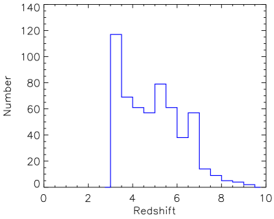
Figure 1: Redshift distribution of 572 spectra (522 galaxies) with high S/Ns in our sample. The sample covers a redshift range of $3.0<z<9.5$, with 267 spectra at $z>5$.

3 Results

In this section we measure $\Delta\alpha/\alpha$ and constrain the spacetime variation of $\alpha$ at $z>3$. We basically follow the procedure in our previous work (Jiang et al., 2024). The wavelength calibration is a key step to achieve the high accuracy of wavelength measurements, so previous studies paid close attention to it. In Jiang et al. (2024), the galaxy sample is very large, so the uncertainties of the $\Delta\alpha/\alpha$ measurements are dominated by systematics associated with the wavelength calibration. Compared to the DESI data in Jiang et al. (2024), the galaxy sample in this work is much smaller, and the spectral resolutions and S/Ns of the lines are lower. Therefore, we expect that the final $\Delta\alpha/\alpha$ uncertainties would be dominated by measurement errors instead of systematics. But we will show in Section 3.3 that systematics are still important. We will discuss the uncertainties of $\Delta\alpha/\alpha$ in Section 4.

3.1 Methodology

We first calculate $\Delta\alpha/\alpha$ for individual spectra or galaxies using the [O III] doublet lines based on the AD method. We use $\lambda_{1}$, $\lambda_{2}$, and $\bar{\lambda}$ to denote the two line wavelengths in vacuum and their average value. With a non-relativistic approximation for light elements, the wavelength separation of the doublet lines $\Delta\lambda=\lambda_{2}-\lambda_{1}$ is directly related to $\alpha$ via $\Delta\lambda/\bar{\lambda}\propto\alpha^{2}$. As we did in Jiang et al. (2024), we replace $\bar{\lambda}$ by $\lambda_{2}$, because the [O III] $\lambda$5007 line is much stronger and thus has a much higher S/N than the [O III] $\lambda$4959 line. This does not change the result. Then $\Delta\alpha/\alpha$ is calculated by

$$\Delta\alpha/\alpha\approx 0.5\times\left(\frac{\Delta\lambda(z_{2})/\lambda_{2}(z_{2})}{\Delta\lambda(z_{1})/\lambda_{2}(z_{1})}-1\right),$$ (1)

where $z_{1}$ and $z_{2}$ label two redshifts. Equation 1 measures the relative $\alpha$ variation at any two redshifts. One can see that any uniform shift of a spectrum caused by a cosmological redshift or a Doppler effect does not affect the $\Delta\alpha/\alpha$ measurement, meaning that this measurement strongly depends on the relative wavelength calibration. The absolute wavelength calibration is less important, and this is one major advantage of the AD method.

In Jiang et al. (2024), we have demonstrated the great power of [O III] for the $\Delta\alpha/\alpha$ measurement, owing to the wide wavelength separation between the two doublet lines and its strong emission in many galaxies. The wavelength separation $\Delta\lambda$ is directly proportional to the sensitivity of the $\Delta\alpha/\alpha$ measurement, because Equation 1 can be rewritten as

$$\Delta\alpha/\alpha\approx 0.5\times\delta(\Delta\lambda)/\Delta\lambda,$$ (2)

where $\delta(\Delta\lambda)=\Delta\lambda(z_{2})-\Delta\lambda(z_{1})$. The wavelength separation of [O III] in the rest frame is nearly 50 Å, roughly one order of magnitude larger than most fine-structure doublet lines in the UV and optical.

Previous studies used the present-day wavelengths as the reference values. Following these studies, we assume $z_{1}=0$, then the two reference values are $\lambda_{1}(0)=4960.295$ Å and $\lambda_{2}(0)=5008.240$ Å, respectively. As we emphasized above, the absolute values are not critical, because Equation 1 compares any two emission line systems at any two redshifts.

3.2 Measurement of $\Delta\alpha/\alpha$

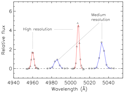
Figure 2: Example of a single Gaussian fit to [O III] in two spectra of one galaxy, including a medium-resolution spectrum and a high-resolution spectrum. The medium-resolution spectrum has been shifted by 25 Å (in the rest frame) for clarity. The triangles and squares represent the data points and the underlying continuum emission has been subtracted. The red and blue profiles are the best Gaussian fits.

We measure the wavelengths of the emission lines and calculate $\Delta\alpha/\alpha$ for individual spectra based on Equation 1. The two [O III] doublet emission lines intrinsically have the identical line profiles since both transitions are from the same excited energy level of double-ionized oxygen. In reality, they could have slightly different profiles in an observed spectrum due to different spectral resolutions and dispersions in different wavelength ranges. We use a single Gaussian profile to fit individual [O III] lines and obtain the line wavelengths from the best fits.

For each emission line, we first subtract its underlying continuum emission by fitting a second-order polynomial curve to a short spectral range around the line. After the continuum subtraction, we fit a single Gaussian to the line. The two [O III] doublet lines are fitted independently. Figure 2 shows an example of our best fits in two spectra of one galaxy, including a medium-resolution spectrum and a high-resolution spectrum (medium- and high-resolution are relative). The results are quite good. As we found in Jiang et al. (2024), a single Gaussian is sufficient to model narrow [O III] lines under the DESI resolution ($R=4000\sim 5000$), but a double Gaussian is preferred when lines are broader. In this work, our spectral resolutions are lower, so a single Gaussian works well for our galaxies.

With the measured wavelengths above, we calculate $\Delta\alpha/\alpha$ using Equation 1. Figure 3 shows an example of the $\Delta\alpha/\alpha$ values from individual spectra at $6<z<7$. The $\Delta\alpha/\alpha$ uncertainty of a spectrum is the combination in quadrature of a measurement error and a systematic error from the wavelength calibration. We have neglected the systematic error so far. The measurement error is estimated by Equation 1 from the propagation of the errors of the two line wavelengths. To suppress significant impact from a tiny fraction of individual spectra, we remove those whose $\Delta\alpha/\alpha$ values deviate from zero by more than $10\sigma$. Such strong detections for individual objects are almost certainly caused by non-physical reasons. There is only one spectrum/galaxy that meets this criterion and is excluded.

Figure 3: An example of measured $\Delta\alpha/\alpha$ values from individual spectra at $6<z<7$.

Figure 4 shows the distributions of the $\Delta\alpha/\alpha$ values in four redshift ranges. The distributions are generally symmetric, except the one in the second panel for $4<z<5$ that is slightly skewed with higher numbers at lower values. This asymmetric distribution naturally leads to a slightly negative $\Delta\alpha/\alpha$ value, as we will see in the next subsection.

3.3 Time Variation of $\alpha$

In order to estimate the time variation of $\alpha$, we divide the sample into five subsamples in the following five redshift bins, $3<z<4$, $4<z<5$, $5<z<6$, $6<z<7$, and $z>7$. For each redshift bin, we calculate $\Delta\alpha/\alpha$ and its error using two methods. In the first method, we take a weighted average. In the second method, we use a bootstrap estimate. For a redshift bin with $n$ galaxies, its $\Delta\alpha/\alpha$ and error are estimated from 10,000 simulated samples. To generate a simulated sample, we randomly draw $n$ galaxies with replacement from the real galaxies in this redshift bin, and calculate the weighted average of $\Delta\alpha/\alpha$ for the simulated sample. If we assume that the weighted averages from the 10,000 simulated samples obey a Gaussian distribution, then the $\Delta\alpha/\alpha$ and error values of this redshift bin are the mean and standard deviation of this Gaussian distribution.

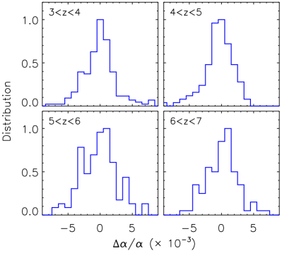
Figure 4: Distributions of $\Delta\alpha/\alpha$ for individual spectra in four redshift ranges. Each histogram has been normalized so that the peak value is 1.

Figure 5 displays the results from the two methods. They are well consistent, except that the errors from the bootstrap method are about twice larger. The bootstrap method is usually more robust, because it is less sensitive to individual errors (which could be underestimated or overestimated). The discrepancy between the errors can be caused by different reasons, such as the sample size and systematics associated with the wavelength calibration. The bootstrap estimate works better for larger sample sizes. In Jiang et al. (2024), the sample size or the sizes of subsamples are very large and the spectra are homogeneous in terms of S/Ns, so the errors from the two methods are well consistent. In this work, the sample sizes are much smaller and the spectra are quite heterogeneous. In a few subsamples, the weighted averages of the simulated samples apparently deviate from a Gaussian distribution. Nevertheless, the bootstrap method should have provided us with a reliable estimate of the upper limits of the errors. On the contrary, the weighted average method may have underestimated the errors, because a high-accuracy wavelength calibration for JWST is challenging and we did not consider any systematics associated with the wavelength calibration. We will discuss the errors of $\Delta\alpha/\alpha$ in Section 4.

Figure 5 shows that the $1\sigma$ errors of $\Delta\alpha/\alpha$ in individual redshift bins are roughly $(1-2)\times 10^{-4}$, depending on the methods adopted. It further suggests a non-variation of $\alpha$ (within $1\sigma$) in all redshift ranges. We also calculate $\Delta\alpha/\alpha$ for the whole sample and the values are $(0.4\pm 0.4)\times 10^{-4}$ and $(0.4\pm 0.7)\times 10^{-4}$ from the two methods, respectively. The magenta and black squares (arbitrarily placed at $z=6$ in Figure 5) indicate the two measurements. These constraints are not as strong as those from observations of lower-redshift objects, particularly quasar absorption lines. However, previous studies rarely reached the redshift range of $z>4$, and here we provide the first constraints on the $\alpha$ variation at the highest redshifts up to $z>9$. Future JWST observations will provide more stringent constraint.

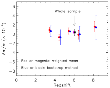
Figure 5: Relative $\alpha$ variation $\Delta\alpha/\alpha$ with redshift. The red and blue circles represent the results from the weighted average and bootstrap estimate methods, respectively. The results from the two methods are well consistent, except that the errors from the bootstrap method are larger. The magenta and black squares, arbitrarily placed at $z=6$, represent the result for the whole sample. The figure shows no apparent $\alpha$ variation (within $1\sigma$) with time.

3.4 Spatial Variation of $\alpha$

We briefly test the spatial variation of $\alpha$. Some previous studies found tentative evidence for a possible variation of $\Delta\alpha/\alpha$ in space at a level below $10^{-5}$ (e.g., Webb et al., 2011; King et al., 2012). In Jiang et al. (2024), we used a large number of galaxies over a few thousand deg² at $z<1$ and did not find an apparent variation of $\alpha$ at a level of $<10^{-4}$. In this work, we do not have a sufficiently large sample or a sufficiently high accuracy of $\Delta\alpha/\alpha$ to perform a detailed analysis. Instead, we compare four $\Delta\alpha/\alpha$ values for four fields, including CEERS (14h20m, +52d58m), GOODS-S (03h32m, $-$27d49m), GOODS-N (12h36m, +62d15m), and A2744 (00h14m, $-$30d25m). The spectra in these fields dominate our sample, and they cover a similar redshift range. We calculate their $\Delta\alpha/\alpha$ values using the bootstrap method and the result is shown in Figure 6. The calculated $\Delta\alpha/\alpha$ values for the GOODS-N and A2744 fields are well consistent with zero. The $\Delta\alpha/\alpha$ values for the GOODS-S and CEERS fields marginally deviate from zero, but are still consistent within a $1\sigma$ level of $\sim 10^{-4}$. The small deviation is likely caused by systematics associated with the wavelength calibration (see discussions below).

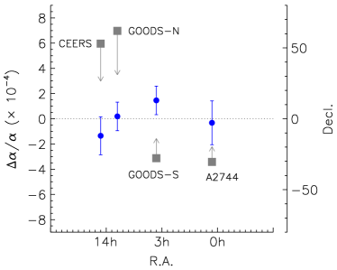
Figure 6: Spatial variation of $\Delta\alpha/\alpha$. The blue circles represent the results from the bootstrap method for four fields, including CEERS, GOODS-S, GOODS-N, and A2744. The coordinates of the fields are indicated by the gray squares: the $x$-axis only shows the R.A. values of our interest, and the $y$-axis on the right shows declination. The figure shows that the four $\Delta\alpha/\alpha$ values are roughly consistent with zero within $1\sigma$.

4 Discussion

The calculation of $\Delta\alpha/\alpha$ relies on the wavelength measurement of emission lines. The uncertainty of $\Delta\alpha/\alpha$ is mainly the combination in quadrature of a measurement error and a systematic error originated from the wavelength calibration. We did not consider the latter in this work. It is often challenging to obtain a high-accuracy wavelength calibration for space missions. Figure 5 shows that the uncertainties from the bootstrap method are roughly twice larger than those from the weighted mean method. We proposed a few explanations for the discrepancy, but the major reason is likely to be the wavelength calibration, i.e., the weighted mean method has probably underestimated the errors. In other words, the uncertainties from the wavelength calibration that we did not consider are comparable to the measurement errors. We discuss them below.

Equation 1 indicates that our calculation of $\Delta\alpha/\alpha$ depends on the absolute wavelength $\lambda_{2}$ and the wavelength difference $\Delta\lambda$, but it is much more sensitive to the latter. We first estimate the effect of the absolute wavelength calibration. The NIRCam WFSS absolute wavelength calibration is accurate to about 1–2 nm for a line at around 4 $\mu$m (e.g., Sun et al., 2023; Torralba-Torregrosa et al., 2024). Using Equation 1, this corresponds to an uncertainty of about $2\times 10^{-4}$ for individual $\Delta\alpha/\alpha$ measurements. The absolute wavelength calibration for the NIRSpec MOS spectra is a few times better (e.g., D’Eugenio et al., 2024), suggesting an uncertainty of $<0.5\times 10^{-4}$ on $\Delta\alpha/\alpha$. It is worth mentioning that our sample is completely dominated by the NIRSpec MOS spectra. If this uncertainty is statistically random, then its effect should be significantly suppressed for large samples. Therefore, this uncertainty from the absolute wavelength calibration is negligible, given that the typical $\Delta\alpha/\alpha$ uncertainties seen in Figures 5 and 6 are about $(1-2)\times 10^{-4}$.

The calculation of $\Delta\alpha/\alpha$ is very sensitive to the relative wavelength calibration or the wavelength difference $\Delta\lambda$. Equation 2 shows that a change of 0.1 Å in $\Delta\lambda$ for [O III] leads to $\Delta\alpha/\alpha\approx 10^{-3}$, meaning that a wavelength distortion of 0.1 Å in the rest frame (or 0.4–1 Å in the observed frame for our sample) between the two doublet lines will cause a variation of $\Delta\alpha/\alpha\approx 10^{-3}$. Note that 0.4–1 Å corresponds to several percent of one pixel in the JWST spectra. Such a small wavelength uncertainty is highly possible, thought the JWST wavelength calibration has not been fully understood. If this uncertainty is statistically random, then its effect can be reduced by large samples. Figure 6 shows that two $\Delta\alpha/\alpha$ data points marginally deviate from zero by $\sim 1\sigma$. It is presumably caused by this uncertainty from the relative wavelength calibration. In other words, this uncertainty is not completely random, and thus introduces small systematical biases at a level of $\sim 10^{-4}$.

Despite that the uncertainties from the wavelength calibration are non-negligible, they should be very small. Their introduced systematical biases are at a level of $\Delta\alpha/\alpha\sim 10^{-4}$, corresponding to a wavelength distortion of $0.04\sim 0.1$ Å in the observed spectra. If the systematical uncertainties are larger, we would have seen a significant detection of $\Delta\alpha/\alpha$. This implies that the wavelength calibration for the current JWST spectra is quite robust.

5 Summary

We have used a sample of high-redshift [O III] emission-line galaxies to constrain the spacetime variation of $\alpha$ at redshift $3<z<10$. The sample consists of 572 JWST spectra with high S/Ns from 522 galaxies. The sample was divided into 5 subsamples based on redshift and $\Delta\alpha/\alpha$ was calculated for the individual subsamples using two methods. We found that the calculated $\Delta\alpha/\alpha$ values are all consistent with zero within $1\sigma$ error of $(1-2)\times 10^{-4}$. A stronger constraint was achieved to be $\Delta\alpha/\alpha=(0.4\pm 0.7)\times 10^{-4}$ when the whole sample was used. We also briefly tested the spatial variation in $\alpha$ using galaxies in four directions on the sky and the $\Delta\alpha/\alpha$ values in different directions are also consistent with zero at a $1\sigma$ level of $\sim 10^{-4}$. Our results suggest no strong variation in $\alpha$ over a wide redshift range up to $z\sim 9.5$. This is the first constraint on $\alpha$ using the highest-redshift objects. We also found that the systematical errors from the wavelength calibration in the JWST spectra are non-negligible but small, and they did not introduce obvious systematical biases. As JWST is accumulating data at a fast pace, we expect to have a much larger dataset and put stronger constraints on $\Delta\alpha/\alpha$ in the future.

References

- Albareti et al. (2015) Albareti, F. D., Comparat, J., Gutiérrez, C. M., et al. 2015, MNRAS, 452, 4153, doi: 10.1093/mnras/stv1406
- Alves et al. (2018) Alves, C. S., Leite, A. C. O., Martins, C. J. A. P., et al. 2018, Phys. Rev. D, 97, 023522, doi: 10.1103/PhysRevD.97.023522
- Arrabal Haro et al. (2023) Arrabal Haro, P., Dickinson, M., Finkelstein, S. L., et al. 2023, ApJ, 951, L22, doi: 10.3847/2041-8213/acdd54
- Bahcall & Schmidt (1967) Bahcall, J. N., & Schmidt, M. 1967, Phys. Rev. Lett., 19, 1294, doi: 10.1103/PhysRevLett.19.1294
- Bahcall et al. (2004) Bahcall, J. N., Steinhardt, C. L., & Schlegel, D. 2004, ApJ, 600, 520, doi: 10.1086/379971
- Barrow et al. (2002) Barrow, J. D., Sandvik, H. B., & Magueijo, J. 2002, Phys. Rev. D, 65, 063504, doi: 10.1103/PhysRevD.65.063504
- Brammer (2022) Brammer, G. 2022, msaexp: NIRSpec analyis tools, 0.3.4, Zenodo, doi: 10.5281/zenodo.7313329
- Bunker et al. (2023) Bunker, A. J., Cameron, A. J., Curtis-Lake, E., et al. 2023, arXiv e-prints, arXiv:2306.02467, doi: 10.48550/arXiv.2306.02467
- Chand et al. (2005) Chand, H., Petitjean, P., Srianand, R., & Aracil, B. 2005, A&A, 430, 47, doi: 10.1051/0004-6361:20041186
- Cowie & Songaila (1995) Cowie, L. L., & Songaila, A. 1995, ApJ, 453, 596, doi: 10.1086/176422
- Damour & Dyson (1996) Damour, T., & Dyson, F. 1996, Nuclear Physics B, 480, 37, doi: 10.1016/S0550-3213(96)00467-1
- DESI Collaboration et al. (2022) DESI Collaboration, Abareshi, B., Aguilar, J., et al. 2022, AJ, 164, 207, doi: 10.3847/1538-3881/ac882b
- DESI Collaboration et al. (2023a) DESI Collaboration, Adame, A. G., Aguilar, J., et al. 2023a, arXiv e-prints, arXiv:2306.06308, doi: 10.48550/arXiv.2306.06308
- DESI Collaboration et al. (2023b) —. 2023b, arXiv e-prints, arXiv:2306.06307, doi: 10.48550/arXiv.2306.06307
- D’Eugenio et al. (2024) D’Eugenio, F., Cameron, A. J., Scholtz, J., et al. 2024, arXiv e-prints, arXiv:2404.06531. https://arxiv.org/abs/2404.06531
- Dumont & Webb (2017) Dumont, V., & Webb, J. K. 2017, MNRAS, 468, 1568, doi: 10.1093/mnras/stx381
- Dzuba et al. (1999) Dzuba, V. A., Flambaum, V. V., & Webb, J. K. 1999, Phys. Rev. Lett., 82, 888, doi: 10.1103/PhysRevLett.82.888
- Eisenstein et al. (2023) Eisenstein, D. J., Willott, C., Alberts, S., et al. 2023, arXiv e-prints, arXiv:2306.02465, doi: 10.48550/arXiv.2306.02465
- Evans et al. (2014) Evans, T. M., Murphy, M. T., Whitmore, J. B., et al. 2014, MNRAS, 445, 128, doi: 10.1093/mnras/stu1754
- Finkelstein et al. (2023) Finkelstein, S. L., Bagley, M. B., Ferguson, H. C., et al. 2023, ApJ, 946, L13, doi: 10.3847/2041-8213/acade4
- Gaia Collaboration et al. (2023) Gaia Collaboration, Vallenari, A., Brown, A. G. A., et al. 2023, A&A, 674, A1, doi: 10.1051/0004-6361/202243940
- Heintz et al. (2024) Heintz, K. E., Brammer, G. B., Watson, D., et al. 2024, arXiv e-prints, arXiv:2404.02211, doi: 10.48550/arXiv.2404.02211
- Jiang et al. (2024) Jiang, L., Pan, Z., Aguilar, J. N., et al. 2024, arXiv e-prints, arXiv:2404.03123, doi: 10.48550/arXiv.2404.03123
- King et al. (2012) King, J. A., Webb, J. K., Murphy, M. T., et al. 2012, MNRAS, 422, 3370, doi: 10.1111/j.1365-2966.2012.20852.x
- Kotuš et al. (2017) Kotuš, S. M., Murphy, M. T., & Carswell, R. F. 2017, MNRAS, 464, 3679, doi: 10.1093/mnras/stw2543
- Lee et al. (2023) Lee, C.-C., Webb, J. K., Carswell, R. F., et al. 2023, MNRAS, 521, 850, doi: 10.1093/mnras/stad600
- Martins (2017) Martins, C. J. A. P. 2017, Reports on Progress in Physics, 80, 126902, doi: 10.1088/1361-6633/aa860e
- Milaković et al. (2021) Milaković, D., Lee, C.-C., Carswell, R. F., et al. 2021, MNRAS, 500, 1, doi: 10.1093/mnras/staa3217
- Molaro et al. (2013) Molaro, P., Centurión, M., Whitmore, J. B., et al. 2013, A&A, 555, A68, doi: 10.1051/0004-6361/201321351
- Murphy et al. (2022) Murphy, M. T., Berke, D. A., Liu, F., et al. 2022, Science, 378, 634, doi: 10.1126/science.abi9232
- Murphy et al. (2001a) Murphy, M. T., Webb, J. K., Flambaum, V. V., Churchill, C. W., & Prochaska, J. X. 2001a, MNRAS, 327, 1223, doi: 10.1046/j.1365-8711.2001.04841.x
- Murphy et al. (2001b) Murphy, M. T., Webb, J. K., Flambaum, V. V., Prochaska, J. X., & Wolfe, A. M. 2001b, MNRAS, 327, 1237, doi: 10.1046/j.1365-8711.2001.04842.x
- Petrov et al. (2006) Petrov, Y. V., Nazarov, A. I., Onegin, M. S., Petrov, V. Y., & Sakhnovsky, E. G. 2006, Phys. Rev. C, 74, 064610, doi: 10.1103/PhysRevC.74.064610
- Potekhin & Varshalovich (1994) Potekhin, A. Y., & Varshalovich, D. A. 1994, A&AS, 104, 89
- Rosenband et al. (2008) Rosenband, T., Hume, D. B., Schmidt, P. O., et al. 2008, Science, 319, 1808, doi: 10.1126/science.1154622
- Savedoff (1956) Savedoff, M. P. 1956, Nature, 178, 688, doi: 10.1038/178688b0
- Schlafly et al. (2023) Schlafly, E. F., Kirkby, D., Schlegel, D. J., et al. 2023, arXiv e-prints, arXiv:2306.06309, doi: 10.48550/arXiv.2306.06309
- Songaila & Cowie (2014) Songaila, A., & Cowie, L. L. 2014, ApJ, 793, 103, doi: 10.1088/0004-637X/793/2/103
- Sun et al. (2023) Sun, F., Egami, E., Pirzkal, N., et al. 2023, ApJ, 953, 53, doi: 10.3847/1538-4357/acd53c
- Torralba-Torregrosa et al. (2024) Torralba-Torregrosa, A., Matthee, J., Naidu, R. P., et al. 2024, arXiv e-prints, arXiv:2404.10040, doi: 10.48550/arXiv.2404.10040
- Uzan (2011) Uzan, J.-P. 2011, Living Reviews in Relativity, 14, 2, doi: 10.12942/lrr-2011-2
- Wang et al. (2023) Wang, F., Yang, J., Hennawi, J. F., et al. 2023, ApJ, 951, L4, doi: 10.3847/2041-8213/accd6f
- Webb et al. (1999) Webb, J. K., Flambaum, V. V., Churchill, C. W., Drinkwater, M. J., & Barrow, J. D. 1999, Phys. Rev. Lett., 82, 884, doi: 10.1103/PhysRevLett.82.884
- Webb et al. (2011) Webb, J. K., King, J. A., Murphy, M. T., et al. 2011, Phys. Rev. Lett., 107, 191101, doi: 10.1103/PhysRevLett.107.191101
- Webb et al. (2023) Webb, J. K., Lee, C.-C., Milakovic, D., et al. 2023, arXiv e-prints, arXiv:2401.00888, doi: 10.48550/arXiv.2401.00888
- Wilczynska et al. (2015) Wilczynska, M. R., Webb, J. K., King, J. A., et al. 2015, MNRAS, 454, 3082, doi: 10.1093/mnras/stv2148
- Wilczynska et al. (2020) Wilczynska, M. R., Webb, J. K., Bainbridge, M., et al. 2020, Science Advances, 6, eaay9672, doi: 10.1126/sciadv.aay9672