A distribution-free valid p-value for finite samples of bounded random variables

Abstract

We build a valid p-value based on the Pelekis-Ramon-Wang inequality for bounded random variables introduced in [9]. The motivation behind this work is the calibration of predictive algorithms in a distribution-free setting. The super-uniform p-value is tighter than Hoeffding’s and Bentkus’s alternatives in certain regions. Even though we are motivated by a calibration setting in a machine learning context, the ideas presented in this work are also relevant in classical statistical inference. Furthermore, we compare the power of a collection of valid p-values for bounded losses, which are presented in [1].

1 Introduction

In the context of hypothesis testing problems, valid p-values (also known in the literature as super-uniform p-values) offer test statistics that can be used controlling any user-specified significance level. In particular, valid p-values are useful because many multiple testing algorithms use them as an input [3, 7]. Moreover, recent literature has introduced frameworks where valid p-values play a key role to provide rigorous statistical guarantees and uncertainty quantification for a variety of machine learning models [8, 1, 5, 2].

In this work we build upon a concentration inequality from [9], and construct a valid p-value for the calibration of predictive algorithms and multiple testing algorithms. We call this valid p-value the PRW valid p-value (due to Pelekis, Ramon and Wang).

Our work is motivated by applications in predictive inference, particularly, it is motivated by recent work on distribution-free uncertainty quantification for black-box algorithms [1, 4]. On a broader perspective, this work relies on the idea of leveraging concentration inequalities and converting them to obtain valid p-values [4]. Our contribution is mainly concerned with the details of such strategy for a specific concentration inequality. There are variety of concentration inequalities [10] for which these kind of ideas can be replicated with adequate modifications and considerations.

Consider a collection of $n$ independent and identically distributed random variables bounded in $[0,1]$, $L_{1},L_{2},\dots,L_{n}$. We denote $R\coloneq\mathbb{E}(L_{i})\in(0,1)$. We use $\hat{R}$ to denote the sample mean, namely, $\hat{R}\coloneqq\frac{1}{n}\sum_{i=1}^{n}L_{i}$. For example, the random sample $\{L_{i}\}_{i=1}^{n}$ may be associated to the losses of a machine learning model in some calibration set, as in [1]. In such setting we refer to $\hat{R}$ as the empirical risk and $R$ as the theoretical risk. We assume that the latter one is unknown. We may be interested in a hypothesis testing problem:

$$H_{0}:R>\alpha\text{ vs. }H_{1}:R\leq\alpha.$$ (1)

Our objective is to determine if there is statistical significance that a pre-trained predictive algorithm producing losses $\{L_{i}\}_{i=1}^{n}$ on a calibration set has a risk (expected loss) below some specified level $\alpha\in(0,1)$.

The motivation for this work from the perspective of classical statistical inference is a setting where we would like to do a hypothesis test for the mean of a collection of $n$ i.i.d. random variables as in 1, where we do not know any other information about the generating distribution other than the fact that its support is a subset of the interval $[0,1]$. The random variables can be either discrete of continuous.

2 Main results

Let us begin considering Theorem 1.8 from [9], for the special case where the involved random variables are all identically distributed.

Theorem 2.1

Let $X_{1},\dots,X_{n}$ be independent and identically distributed (i.i.d.) random variables such that $0\leq X_{i}\leq 1$ and $p\coloneqq\mathbb{E}[X_{i}]$. Let $n\in\mathbb{N}$, $p\in(0,1)$ and $Bin(n,p)$ denote a Binomial random variable with parameters $(n,p)$. Then for any positive integer $t$ such that $np<t\leq n$,

$$\mathbb{P}\Big{(}\sum_{i=1}^{n}X_{i}\geq t\Big{)}\leq\frac{t-tp}{t-np}\mathbb{P}\{Bin(n,p)\geq t\}.$$

Just as the authors of [9] point out, for certain values of $p,n,\text{ and }t$ this upper bound is smaller than the one provided by Bentkus in his celebrated inequality [6]. We will verify those observations in the valid p-value formulation in the last section of this paper.

A classical idea for many concentration inequalities is that the results that hold for a lower tail also hold for the upper tail and vice versa. This is the case for this inequality.

Corollary 2.1.1

(Lower tail version) Let $L_{1},\dots,L_{n}$ be i.i.d. bounded random variables in $[0,1]$, and $R\coloneqq\mathbb{E}(L_{i})\in(0,1)$. Then for any integer $k\in[0,nR)$,

$$\mathbb{P}\Big{(}\sum_{i=1}^{n}L_{i}\leq k\Big{)}\leq\frac{R(n-k)}{nR-k}\mathbb{P}\Big{(}Bin(n,R)\leq k\Big{)}.$$

Proof:

Let $k\in[0,nR)$. Consider a change of variables, $X_{i}\coloneqq 1-L_{i}$, and we take $p\coloneq 1-R$, which is the mean of each $X_{i}$; notice that $p\in(0,1)$ and $0\leq X_{i}\leq 1$ for all $i\in\{1,\dots,n\}$. Also notice that $k\in[0,nR)$ implies $n-k\in(np,n]$.

$$\begin{split}\mathbb{P}\{\sum_{i=1}^{n}L_{i}\leq k\}&=\mathbb{P}\{\sum_{i=1}^{n}(1-X_{i})\leq k\}\\ &=\mathbb{P}\{\sum_{i=1}^{n}X_{i}\geq n-k\}\\ &\leq\frac{n-k-(n-k)(1-R)}{n-k-n(1-R)}\mathbb{P}\{Bin(n,1-R)\geq n-k\}\\ &=\frac{(n-k)R}{nR-k}\mathbb{P}\{n-Bin(n,1-R)\leq k\}\\ &=\frac{(n-k)R}{nR-k}\mathbb{P}\{Bin(n,R)\leq k\}.\end{split}$$

$\square$

We can reformulate this corollary in the following way:

$$\begin{split}\mathbb{P}\{\frac{1}{n}\sum_{i=1}^{n}L_{i}\leq t\}&=\mathbb{P}\{\sum_{i=1}^{n}L_{i}\leq nt\}\\ &\leq\mathbb{P}\{\sum_{i=1}^{n}L_{i}\leq\lceil nt\rceil\}\\ &\leq\frac{R(n-\lceil nt\rceil)}{nR-\lceil nt\rceil}\mathbb{P}\{Bin(n,R)\leq\lceil nt\rceil\},\end{split}$$ (2)

for values of $t\in[0,R)$ such that $0\leq\lceil nt\rceil<nR$. We applied Corollary 2.1.1, and we use the fact that any CDF is non-decreasing. A visual representation of the function $t\mapsto\lceil nt\rceil$ is helpful to understand the upper bound for $t$. We present such representation in Figure 1.

Figure 1: A graph of $\lceil nt\rceil$ in $[0,1]$, with some hypothetical critical values to make sure that the upper bound is well defined. This figure motivates the definition of $\gamma(R)$. The function $\lceil nt\rceil$ takes positive jumps at $\{0,\frac{1}{n},\frac{2}{n},\dots,\frac{n-1}{n}\}$.

Given that $R\in(0,1)$, we have that $0<nR<n$ for any $n\in\mathbb{N}$. Hence, we take

$$\gamma(R)\coloneqq\text{min}\{r\in\mathbb{N}:r\geq nR\}.$$

By the Archimedian Property, the involved set is non-empty. Furthermore, given that the set is not empty, the Well Order Principle guarantees that the minimum always exists. Note the fact that $n$ is always an element in $\{r\in\mathbb{N}:r\geq nR\}$.

Moreover, we consider values of $t\in[0,R)$ such that $t\leq\frac{\gamma(R)-1}{n}$. Note that by definition, $\frac{\gamma(R)-1}{n}<R$. This election of $\gamma(R)$ guarantees that the upper bound for 2 is well defined. Equivalently, what the definition of $\gamma(R)$ helps us ensure is that

$$\Big{[}0,\frac{\gamma(R)-1}{n}\Big{]}\subset\{t\in[0,R):0\leq\lceil nt\rceil<nR\},$$

because by definition, $\gamma(R)-1\notin\{r\in\mathbb{N}:r\geq nR\}$, so

$$t\in\Big{[}0,\frac{\gamma(R)-1}{n}\Big{]}\implies nt\leq\gamma(R)-1<nR\implies\lceil nt\rceil\leq\gamma(R)-1<nR.$$

2.1 Outline

• We will show that if we define $g(t;R)\coloneqq\frac{R(n-\lceil nt\rceil)}{nR-\lceil nt\rceil}\mathbb{P}\{Bin(n,R)\leq\lceil nt\rceil\}$ for all $t\in[0,\frac{\gamma(R)-1}{n})$ and $g(\frac{\gamma(R)-1}{n};R)\coloneqq\text{max}\{1,\frac{R(n-\gamma(R)+1)}{nR-\gamma(R)+1}\mathbb{P}\{Bin(n,R)\leq\gamma(R)-1\}\}$, then we obtain that

  $$g\Big{(}\text{min}\{\hat{R},\frac{\gamma(\alpha)-1}{n}\};\alpha\Big{)}$$

  is a super-uniform p-value to test $H_{0}:R>\alpha$. We will refer to it as PRW valid p-value. We will also provide some plots comparing this valid p-value to Bentkus’s valid p-value and Hoeffding’s tight super-uniform p-value, showing that the PRW valid p-value is tighter than both of them in some regions. As an auxiliary step towards this goal we need intermediate considerations.

• We will show that $g$ has the following properties. Firstly, $g(\cdot;R)$ is a non-decreasing function in its first argument for any fixed value of $R$, for values of $t\in[0,\frac{\gamma(R)-1}{n}]$. For any $R_{1},R_{2}\in(0,1)$ and any $t\in[0,\frac{\gamma(R_{1})-1}{n})$, such that $R_{1}\leq R_{2}$, $g(t;R_{2})\leq g(t;R_{1})$. Moreover, $t\in[0,\frac{\gamma(R_{1})-1}{n})$ implies $t\in[0,\frac{\gamma(R_{2})-1}{n})$ so that we are always in the region where we’ve defined $g$. Finally, for any $\delta\in(0,1)$ such that $\delta>(1-R)^{n}$, we can define

  $$g^{-1}(\delta;R)\coloneqq\text{sup}\Big{\{}t\in\big{[}0,\frac{\gamma(R)-1}{n}\big{]}\quad|\quad g(t;R)\leq\delta\Big{\}}.$$

  And by the fact that $t\mapsto\lceil nt\rceil$ is left continuous and non-decreasing, such supremum is always a maximum and is well defined. Given that $g(0;R)=(1-R)^{n}$, the underlying set is always non-empty for values of $\delta\in(0,1)$ such that $(1-R)^{n}<\delta$.

Lemma 2.2

$g(\cdot;R):[0,\frac{\gamma(R)-1}{n}]\longrightarrow\mathbb{R}$ is non-decreasing for any fixed $R\in(0,1)$.

Proof:

Let $R\in(0,1)$.

Let $t_{1},t_{2}\in[0,\frac{\gamma(R)-1}{n}]$ be such that $t_{1}<t_{2}$ and $k_{j}\coloneqq\lceil nt_{j}\rceil$ for $j=1,2$ such that $k_{2}=k_{1}+1$.

In our first case, we consider $t_{2}<\frac{\gamma(R)-1}{n}$. Then

$$\begin{split}g(t_{1};R)<g(t_{2};R)&\iff\frac{R(n-\lceil nt_{1}\rceil)}{nR-\lceil nt_{1}\rceil}\mathbb{P}\{Bin(n,R)\leq\lceil nt_{1}\rceil\}<\frac{R(n-\lceil nt_{2}\rceil)}{nR-\lceil nt_{2}\rceil}\mathbb{P}\{Bin(n,R)\leq\lceil nt_{2}\rceil\}\\ &\iff\frac{R(n-k_{1})}{nR-k_{1}}\mathbb{P}\{Bin(n,R)\leq k_{1}\}<\frac{R(n-k_{1}-1)}{nR-k_{1}-1}\mathbb{P}\{Bin(n,R)\leq k_{1}+1\}.\\ \end{split}$$

Separately we consider $\mathbb{P}\{Bin(n,R)\leq k_{1}\}<\mathbb{P}\{Bin(n,R)\leq k_{1}+1\}$, which is true by the properties of a CDF of any binomial random variable. Whereas

$$\begin{split}\frac{R(n-k_{1})}{nR-k_{1}}&<\frac{R(n-k_{1}-1)}{nR-k_{1}-1}\iff R(n-k_{1})(nR-k_{1}-1)<R(n-k_{1}-1)(nR-k_{1})\\ &\iff(n-k_{1})(nR-k_{1})-(n-k_{1})<(n-k_{1})(nR-k_{1})-(nR-k_{1})\\ &\iff k_{1}-n<k_{1}-nR\\ &\iff nR<n\\ &\iff R<1.\end{split}$$

We conclude the desired result multiplying both quantities. Moreover this proves that the smallest value that $g(t;R)$ can attain for values of $t\in[0,\frac{\gamma(R)-1}{n}]$ is $g(0;R)=(1-R)^{n}$. And if $t_{2}=\frac{\gamma(R)-1}{n}$, then the same reasoning proves that

$$g(t_{1};R)<\frac{R(n-\lceil nt_{2}\rceil)}{nR-\lceil nt_{2}\rceil}\mathbb{P}\{Bin(n,R)\leq\lceil nt_{2}\rceil\}.$$

And by definition of $g(\frac{\gamma(R)-1}{n};R)$, $\frac{R(n-\lceil nt_{2}\rceil)}{nR-\lceil nt_{2}\rceil}\mathbb{P}\{Bin(n,R)\leq\lceil nt_{2}\rceil\}\leq g(\frac{\gamma(R)-1}{n};R)$, so we can conclude that $g(t_{1};R)<g(t_{2};R)$ when $0\leq t_{1}<t_{2}=\frac{\gamma(R)-1}{n}$. $\square$

Lemma 2.3

$g(t;\cdot):(0,1)\longrightarrow\mathbb{R}$ is non-increasing in $R\in(0,1)$ for any fixed value of $t\in[0,\frac{\gamma(R)-1}{n})$.

Proof:

Let $0<R_{1}<R_{2}<1$. Let $t\in[0,\frac{\gamma(R_{1})-1}{n})$. We notice that

$$0<R_{1}<R_{2}<1\implies\gamma(R_{1})\leq\gamma(R_{2}),$$

by definition of

$$\gamma(R)\coloneqq\text{min}\{r\in\mathbb{N}:r\geq nR\}\text{ for all }R\in(0,1).$$

We have that $\{r\in\mathbb{N}:r\geq nR_{2}\}\subset\{r\in\mathbb{N}:r\geq nR_{1}\}$. So $t\in[0,\frac{\gamma(R_{1})-1}{n})\subseteq[0,\frac{\gamma(R_{2})-1}{n})$.

Let $k\coloneqq\lceil nt\rceil$. Then

$$g(t;R_{2})\leq g(t;R_{1})\iff\frac{R_{2}(n-k)}{nR_{2}-k}\mathbb{P}\{Bin(n,R_{2})\leq k\}\leq\frac{R_{1}(n-k)}{nR_{1}-k}\mathbb{P}\{Bin(n,R_{1})\leq k\}.$$

Clearly, $\mathbb{P}\{Bin(n,R_{2})\leq k\}\leq\mathbb{P}\{Bin(n,R_{1})\leq k\}$. On the other hand, $\frac{R_{2}(n-k)}{nR_{2}-k}\leq\frac{R_{1}(n-k)}{nR_{1}-k}$ if and only if $(nR_{1}-k)R_{2}\leq R_{1}(nR_{2}-k)$. In turn, this occurs if and only if $kR_{1}\leq kR_{2}$, which is true since $k$ is a non-negative integer and $R_{1}<R_{2}$. $\square$

With this context in mind, we introduce the following theorem, which is the main result of this work.

Theorem 2.4

Let $L_{1},\dots,L_{n}$ be a random sample of random variables bounded in $[0,1]$ whose mean is $R\in(0,1)$. Let $\alpha\in(0,1)$. Consider the hypothesis testing problem $H_{0}:R>\alpha\text{ vs. }H_{1}:R\leq\alpha$. Take $\hat{R}\coloneqq\sum\limits_{i=1}^{n}L_{i}$. Then $g\Big{(}\text{min}\{\hat{R},\frac{\gamma(\alpha)-1}{n}\};\alpha\Big{)}$ is a valid p-value to test $H_{0}:R>\alpha$.

Proof:

Let $\delta\in(0,1)$.

Case 1: $\delta\geq(1-R)^{n}$.

Then

$$\begin{split}\mathbb{P}_{H_{0}}\Big{(}g\Big{(}\text{min}\{\hat{R},\frac{\gamma(\alpha)-1}{n}\};\alpha\Big{)}\leq\delta\Big{)}&=\mathbb{P}_{H_{0}}\Big{(}g\Big{(}\text{min}\{\hat{R},\frac{\gamma(\alpha)-1}{n}\};\alpha\Big{)}\leq\delta,\hat{R}\geq\frac{\gamma(\alpha)-1}{n}\Big{)}\\ &+\mathbb{P}_{H_{0}}\Big{(}g\Big{(}\text{min}\{\hat{R},\frac{\gamma(\alpha)-1}{n}\};\alpha\Big{)}\leq\delta,\hat{R}<\frac{\gamma(\alpha)-1}{n}\Big{)},\end{split}$$

where we applied the law of total probability. The event inside the probability of the first term is equal to the empty set due to the fact that by definition $g(\frac{\gamma(\alpha)-1}{n};\alpha)\geq 1$. So we only need to consider the second term.

$$\begin{split}\mathbb{P}_{H_{0}}\Big{(}g\Big{(}\text{min}\{\hat{R},\frac{\gamma(\alpha)-1}{n}\};\alpha\Big{)}\leq\delta\Big{)}&=\mathbb{P}_{H_{0}}\{g\big{(}\hat{R};\alpha\big{)}\leq\delta,\hat{R}<\frac{\gamma(\alpha)-1}{n}\}\\ &\leq\mathbb{P}_{H_{0}}\{g\big{(}\hat{R};R\big{)}\leq\delta,\hat{R}<\frac{\gamma(\alpha)-1}{n}\},\end{split}$$

where we used that $g$ is non-increasing in its second argument for fixed values of its first argument. Next we apply the definition of $g^{-1}$

$$\begin{split}\mathbb{P}_{H_{0}}\{g\big{(}\hat{R};R\big{)}\leq\delta,\hat{R}<\frac{\gamma(\alpha)-1}{n}\}&=\mathbb{P}_{H_{0}}\{\hat{R}\leq g^{-1}(\delta;R),\hat{R}<\frac{\gamma(\alpha)-1}{n}\}\\ &\leq\mathbb{P}_{H_{0}}\{\hat{R}\leq g^{-1}(\delta;R)\}\\ &\leq g(g^{-1}(\delta;R);R)\leq\delta.\end{split}$$

Case 2: $\delta<(1-R)^{n}$. Then it is straightforward that

$$\mathbb{P}_{H_{0}}\Big{(}g\Big{(}\text{min}\{\hat{R},\frac{\gamma(\alpha)-1}{n}\};\alpha\Big{)}\leq\delta\Big{)}=0\leq\delta,$$

because the smallest value that $g(t;\alpha)$ can take for values of $t$ such that $t\in[0,\frac{\gamma(\alpha)-1}{n}]$ is $(1-\alpha)^{n}$ and under $H_{0}$, $(1-R)^{n}\leq(1-\alpha)^{n}$. Thus under $H_{0}$, $\delta<(1-R)^{n}$ implies $\delta<(1-\alpha)^{n}$. $\square$

3 A comment on some FWER controlling algorithms

The proposed valid p-value is particularly relevant for regions where the observed empirical risk is much smaller than the considered $\alpha$ in the formulated hypothesis test in 1 as the plots in the Appendix show. This is useful information for the purposes of FWER controlling algorithms that incorporate prior knowledge of the experiments to be carried out, for example in the fixed sequence algorithm and in the fallback procedure [7]. Note that our plots suggest that the PRW super-uniform p-value is not very powerful for values of the empirical risk that are smaller than $\alpha$ but close to it, when comparing it to Bentkus and Hoeffding’s valid p-values. However, we can leverage the fact that the PRW valid p-value is very powerful for small observations of the empirical risk. We can leverage this fact when implementing a fixed sequence procedure or a fallback procedure. In the context of those algorithms, given the provided order for the null hypotheses, it suggests that the observed valid p-values using the PRW valid p-value will be smaller than Bentkus’s and Hoeffding’s valid p-values for many of the first nulls, hence increasing the power of the algorithms.

Appendix

We study some properties of $g^{-1}(\delta;R)\coloneqq\text{sup}\Big{\{}t\in\big{[}0,\frac{\gamma(R)-1}{n}\big{]}\quad|\quad g(t;R)\leq\delta\Big{\}}$, for values of $\delta\in[(1-R)^{n},1)$. By definition, $(1-R)^{n}=g(0;R)$, thus $0\in\Big{\{}t\in\big{[}0,\frac{\gamma(R)-1}{n}\big{]}\quad|\quad g(t;R)\leq\delta\Big{\}}$. Moreover, since $\Big{\{}t\in\big{[}0,\frac{\gamma(R)-1}{n}\big{]}\quad|\quad g(t;R)\leq\delta\Big{\}}\subset\big{[}0,\frac{\gamma(R)-1}{n}\big{]}$, then the set of interest is bounded above and by he Axiom of Completeness, $g^{-1}(\delta;R)$ is defined. Furthermore, $g^{-1}(\delta;R)\leq\text{sup}\big{[}0,\frac{\gamma(R)-1}{n}\big{]}=\frac{\gamma(R)-1}{n}$. And by definition $g(\frac{\gamma(R)-1}{n};R)\geq 1$, thus $\frac{\gamma(R)-1}{n}\notin\Big{\{}t\in\big{[}0,\frac{\gamma(R)-1}{n}\big{]}\quad|\quad g(t;R)\leq\delta\Big{\}}$. We want to show that $g^{-1}(\delta;R)\in\Big{\{}t\in\big{[}0,\frac{\gamma(R)-1}{n}\big{]}\quad|\quad g(t;R)\leq\delta\Big{\}}$. That is, $g^{-1}(\delta;R)$ is a maximum. By contradiction suppose that $g(g^{-1}(\delta;R);R)>\delta$. But given that for any fixed $R\in(0,1)$, $g(t;R)$ is continuous from the left and has a step function form, $\exists\epsilon>0$ sufficiently small such that $g(g^{-1}(\delta;R)-\epsilon;R)=g(g^{-1}(\delta;R);R)>\delta$. And given that $g(t;R)$ is non-decreasing, then $t\leq g^{-1}(\delta;R)-\epsilon$ for all $t\in\Big{\{}x\in\big{[}0,\frac{\gamma(R)-1}{n}\big{]}:g(x;R)\leq\delta\Big{\}}$. But this contradicts that $g^{-1}(\delta;R)$ is a supremum. We conclude that $g(g^{-1}(\delta;R);R)\leq\delta$.

Theorem 2.1 holds for $t=n$

If the involved random variables are continuous, it is then immediate that

$$\mathbb{P}\Big{(}\sum_{i=1}^{n}X_{i}\geq t\Big{)}\leq\frac{t-tp}{t-np}\mathbb{P}\{Bin(n,p)\geq t\},$$

because this inequality for $t=n$ simplifies to

$$\mathbb{P}\Big{(}\sum_{i=1}^{n}X_{i}\geq n\Big{)}=\mathbb{P}\Big{(}\bigcap_{i=1}^{n}\{X_{i}=1\}\Big{)}=0\leq\mathbb{P}\{Bin(n,p)\geq n\}.$$

Whereas in the discrete case, consider $Y_{i}\overset{i.i.d.}{\sim}Bernoulli(p)$, for $i\in\{1,\dots,n\}$.

$$\begin{split}\mathbb{P}\Big{(}\sum_{i=1}^{n}X_{i}\geq n\Big{)}&=\mathbb{P}\Big{(}\bigcap_{i=1}^{n}\{X_{i}=1\}\Big{)}\\ &=\mathbb{P}(X_{1}=1)^{n}.\end{split}$$

On the other hand, the desired upper bound is given by

$$\begin{split}\frac{n-np}{n-np}\mathbb{P}\{Bin(n,p)\geq n\}&=\mathbb{P}\Big{(}\bigcap_{i=1}^{n}\{Y_{i}=1\}\Big{)}\\ &=p^{n}.\end{split}$$

Hence the inequality holds in the discrete case if and only if $\mathbb{P}(X_{1}=1)\leq p$. By definition of $p\coloneq\mathbb{E}\{X_{1}\}$ the result follows:

$$\begin{split}\mathbb{P}(X_{1}=1)\leq\sum_{x\in S_{X_{1}}}x\mathbb{P}(X_{1}=x)=\sum_{x\in S_{X_{1}}-\{1\}}x\mathbb{P}(X_{1}=x)+1\cdot\mathbb{P}(X_{1}=1),\end{split}$$

where $S_{X_{1}}\subseteq[0,1]$ denotes the support of the $X_{i}$’s.

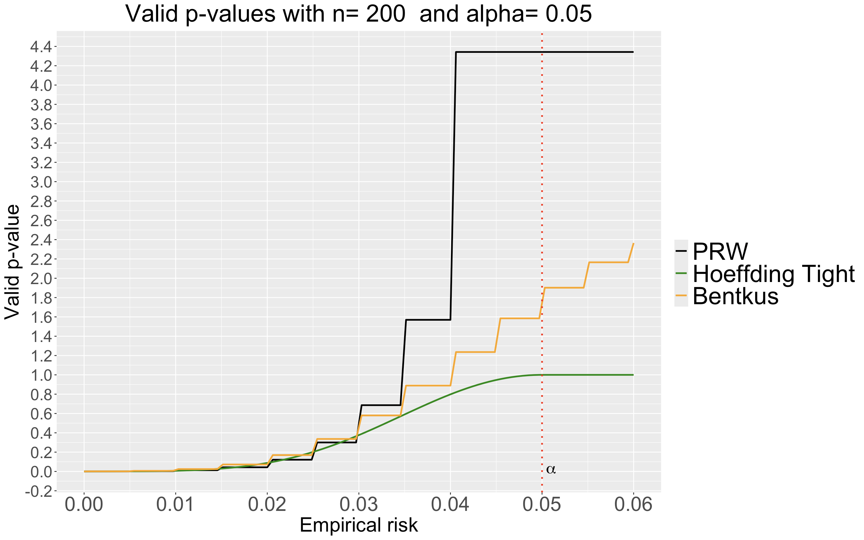
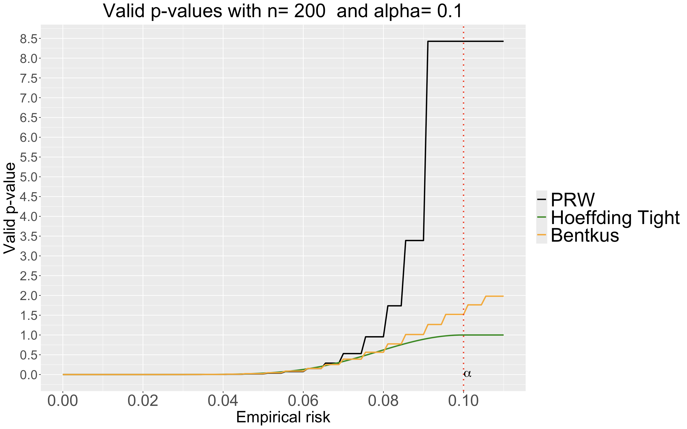
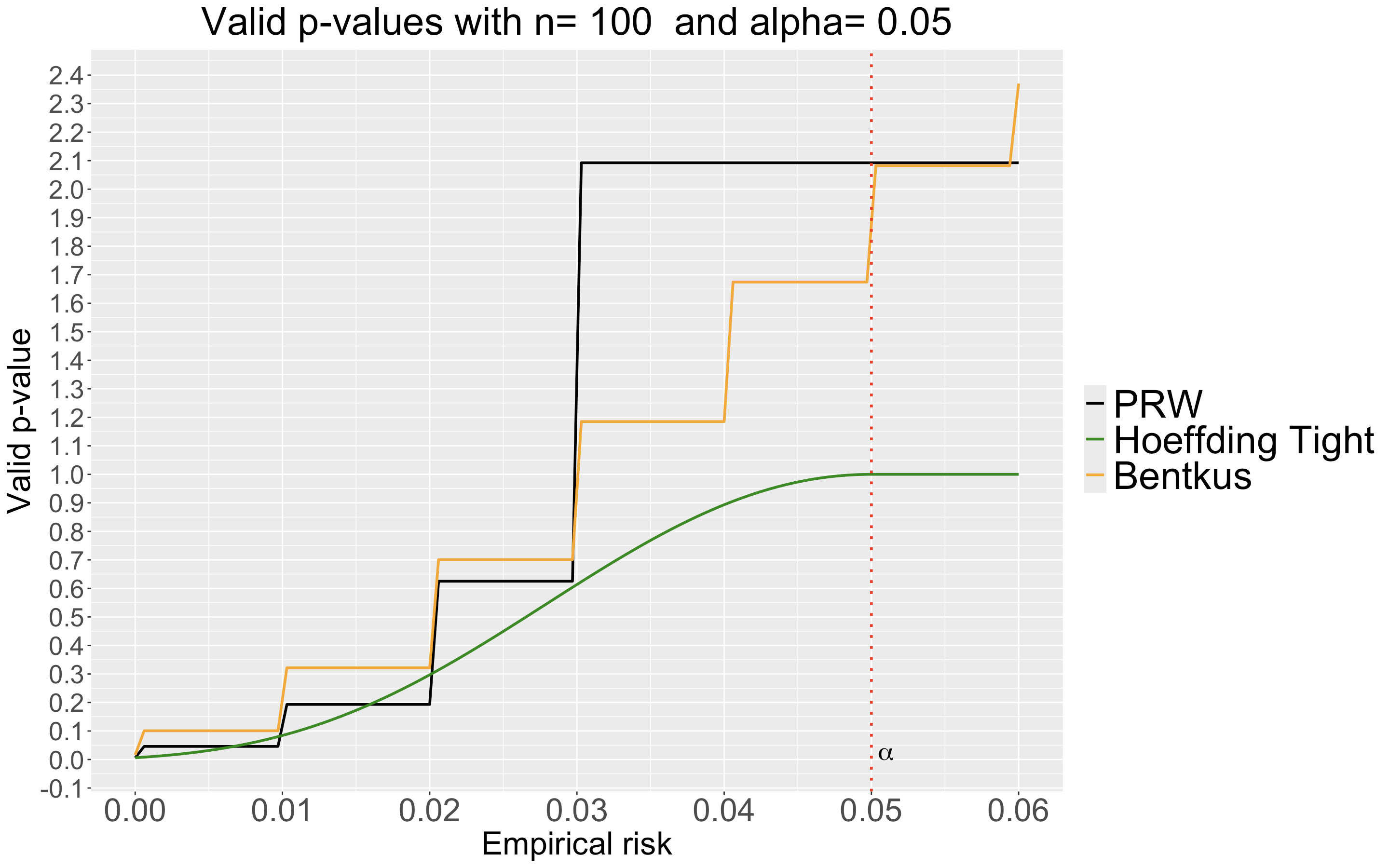
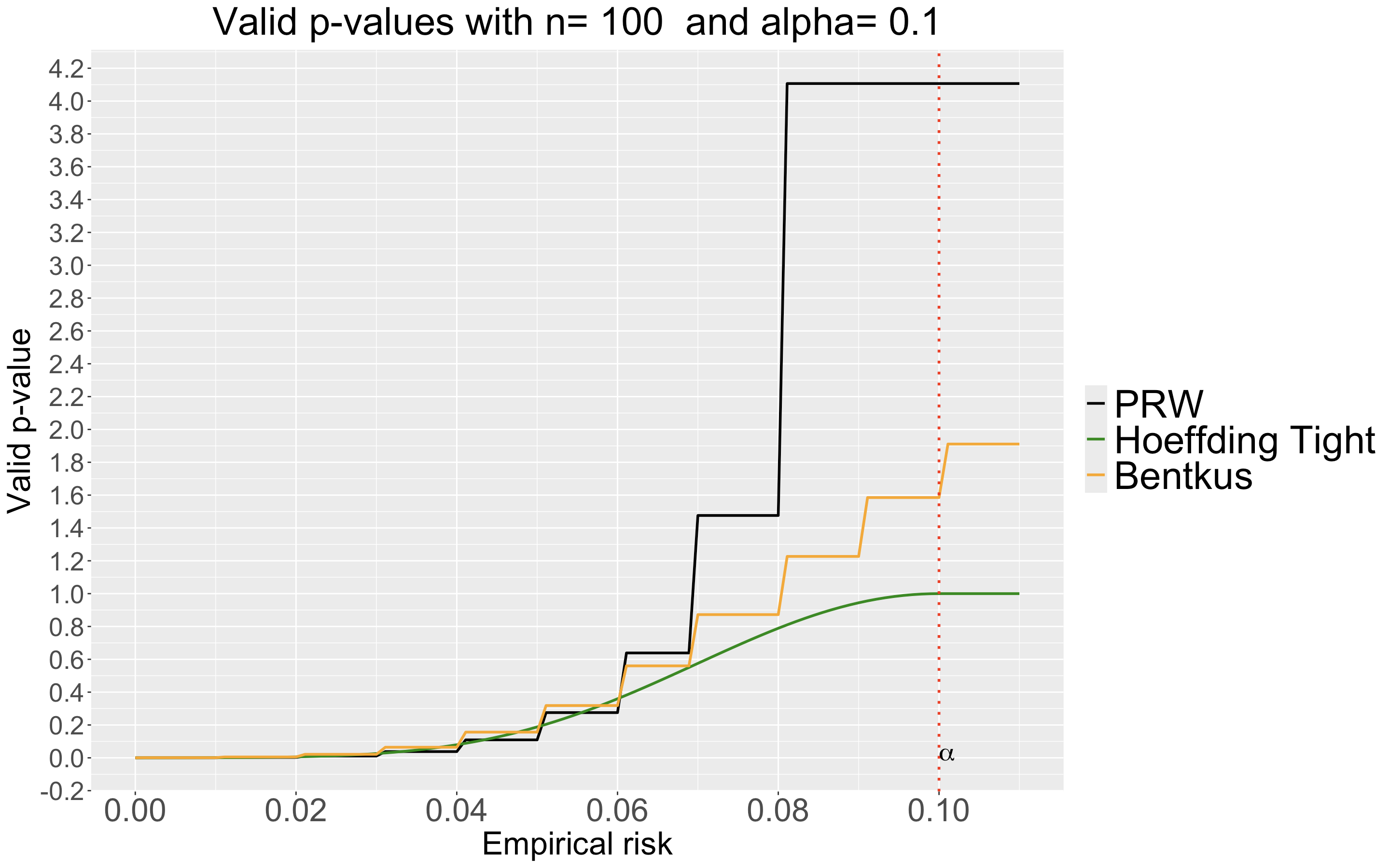
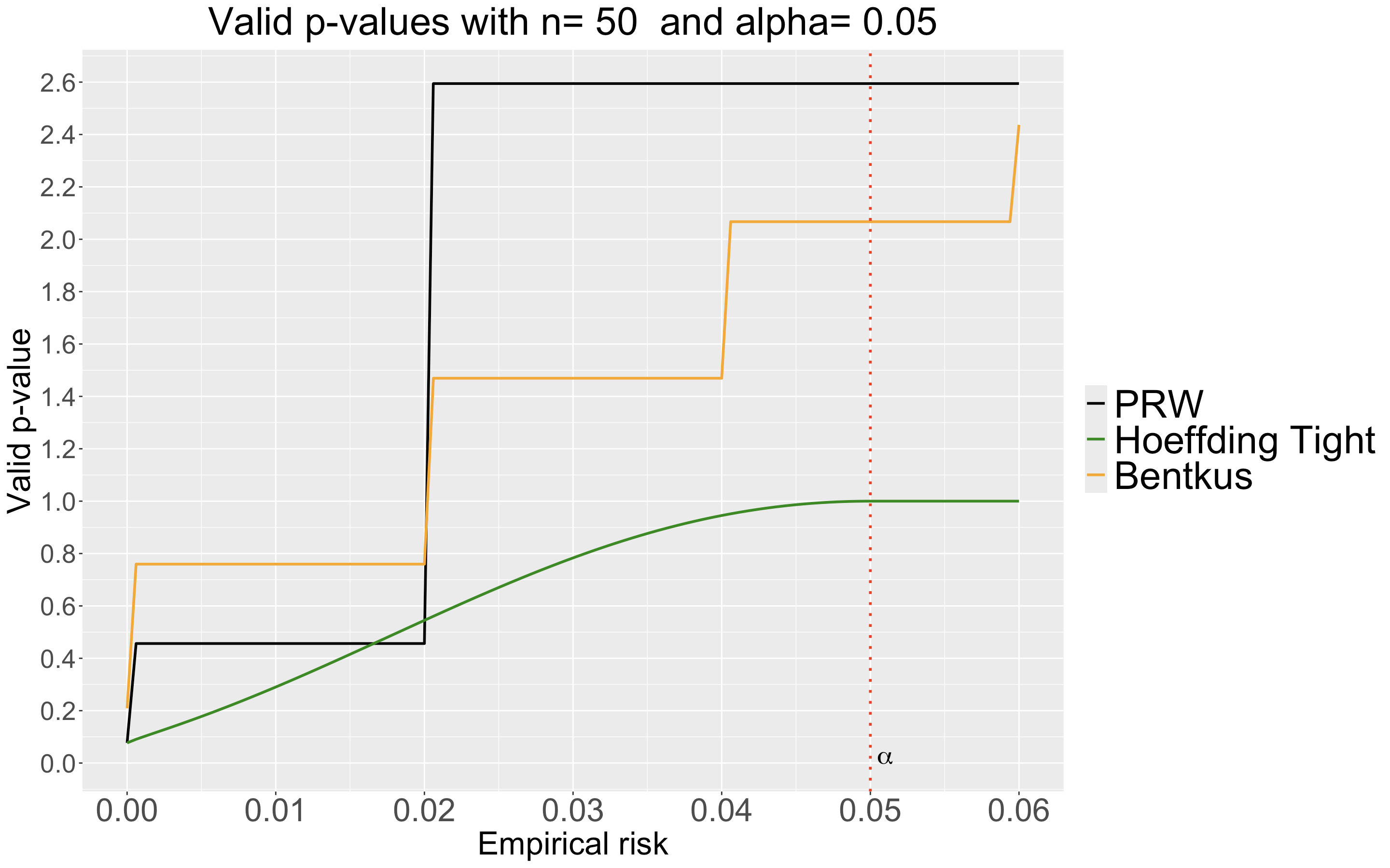
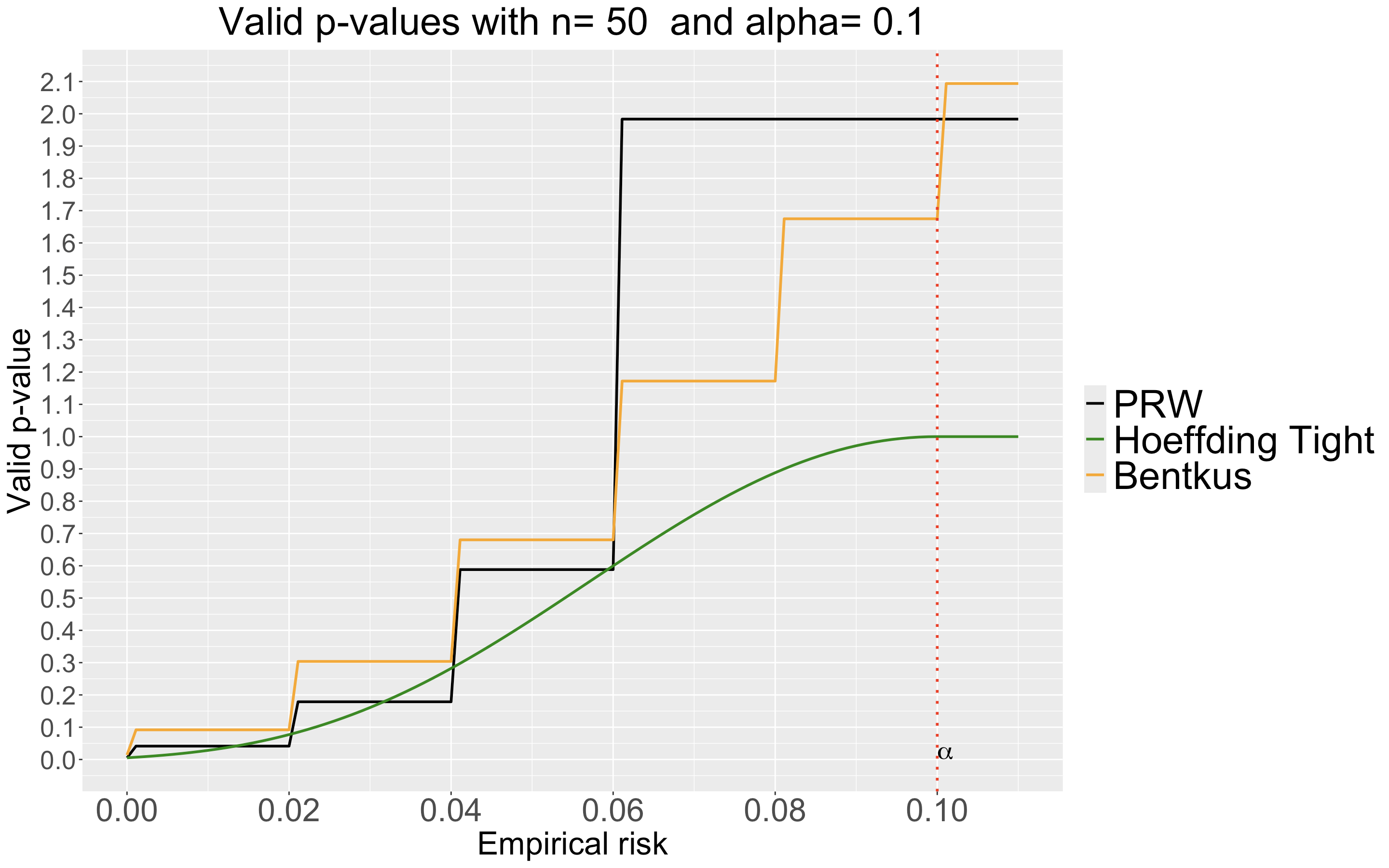
Figure 2: In the same setting as in 1, we consider the following valid p-values as presented in [1] and [4]: $p_{Bent}\coloneqq e\mathbb{P}\{Bin(n,\alpha)\leq\lceil n\hat{R}\rceil\}$, Bentkus’ valid p-value, $p_{HT}\coloneqq exp\Big{\{}-n\Big{(}\text{min}\{\hat{R},\alpha\}log(\frac{\text{min}\{\hat{R},\alpha\}}{\alpha})+(1-\text{min}\{\hat{R},\alpha\})log(\frac{(1-\text{min}\{\hat{R},\alpha\})}{1-\alpha})\Big{)}\Big{\}}$ Hoeffding’s valid p-value (tight version). We consider the valid p-value introduced in this work: $g\Big{(}\text{min}\{\hat{R},\frac{\gamma(\alpha)-1}{n}\};\alpha\Big{)}$, PRW’s valid p-value.

$\hat{R}$	PRW	Hoeffding Tight	Bentkus
0.0000	0.0000	0.0000	0.0001
0.0015	0.0004	0.0001	0.0009
0.0030	0.0004	0.0001	0.0009
0.0045	0.0004	0.0002	0.0009
0.0061	0.0004	0.0003	0.0009
0.0076	0.0004	0.0004	0.0009
0.0091	0.0004	0.0006	0.0009
0.0106	0.0024	0.0009	0.0053
0.0121	0.0024	0.0013	0.0053
0.0136	0.0024	0.0018	0.0053
0.0152	0.0024	0.0024	0.0053
0.0167	0.0024	0.0033	0.0053
0.0182	0.0024	0.0043	0.0053
0.0197	0.0024	0.0056	0.0053
0.0212	0.0109	0.0073	0.0213
0.0227	0.0109	0.0093	0.0213
0.0242	0.0109	0.0117	0.0213
0.0258	0.0109	0.0146	0.0213
0.0273	0.0109	0.0180	0.0213
0.0288	0.0109	0.0221	0.0213
0.0303	0.0379	0.0269	0.0645
0.0318	0.0379	0.0325	0.0645
0.0333	0.0379	0.0389	0.0645
0.0348	0.0379	0.0463	0.0645
0.0364	0.0379	0.0548	0.0645
0.0379	0.0379	0.0643	0.0645
0.0394	0.0379	0.0750	0.0645
0.0409	0.1094	0.0869	0.1565
0.0424	0.1094	0.1002	0.1565
0.0439	0.1094	0.1149	0.1565
0.0455	0.1094	0.1310	0.1565
0.0470	0.1094	0.1485	0.1565
0.0485	0.1094	0.1676	0.1565
0.0500	0.2753	0.1881	0.3185
0.0515	0.2753	0.2102	0.3185
0.0530	0.2753	0.2337	0.3185
0.0545	0.2753	0.2587	0.3185
0.0561	0.2753	0.2851	0.3185
0.0576	0.2753	0.3128	0.3185
0.0591	0.2753	0.3417	0.3185
0.0606	0.6388	0.3718	0.5601
0.0621	0.6388	0.4029	0.5601
0.0636	0.6388	0.4349	0.5601
0.0652	0.6388	0.4677	0.5601
0.0667	0.6388	0.5010	0.5601

Table 1: Values of the p-values across different values of the empirical risk, using $\alpha=0.1,n=100$. Numbers are rounded to 4 decimals.

References

- [1] Anastasios N. Angelopoulos et al. “Learn then Test: Calibrating Predictive Algorithms to Achieve Risk Control”, 2022 arXiv:2110.01052 [cs.LG]
- [2] Anastasios N. Angelopoulos et al. “Prediction-Powered Inference”, 2023 arXiv:2301.09633 [stat.ML]
- [3] Rina Foygel Barber and Emmanuel J. Candès “Controlling the false discovery rate via knockoffs” In The Annals of Statistics 43.5 Institute of Mathematical Statistics, 2015 DOI: 10.1214/15-aos1337
- [4] Stephen Bates et al. “Distribution-Free, Risk-Controlling Prediction Sets”, 2021 arXiv:2101.02703 [cs.LG]
- [5] Stephen Bates et al. “Testing for outliers with conformal p-values” In The Annals of Statistics 51.1 Institute of Mathematical Statistics, 2023 DOI: 10.1214/22-aos2244
- [6] Vidmantas Bentkus “On Hoeffding’s inequalities” In The Annals of Probability 32.2 Institute of Mathematical Statistics, 2004 DOI: 10.1214/009117904000000360
- [7] Alex Dmitrienko, Ajit C Tamhane and Frank Bretz “Multiple testing problems in pharmaceutical statistics”, 2010
- [8] Ziyi Liang, Matteo Sesia and Wenguang Sun “Integrative conformal p-values for powerful out-of-distribution testing with labeled outliers”, 2022 arXiv:2208.11111 [stat.ME]
- [9] Christos Pelekis, Jan Ramon and Yuyi Wang “On the Bernstein-Hoeffding method”, 2015 arXiv:1503.02284 [math.PR]
- [10] Karthik Sridharan “A Gentle Introduction to Concentration Inequalities” URL: https://www.cs.cornell.edu/~sridharan/concentration.pdf