Computation-Aware Kalman Filtering and Smoothing

Abstract

Kalman filtering and smoothing are the foundational mechanisms for efficient inference in Gauss-Markov models. However, their time and memory complexities scale prohibitively with the size of the state space. This is particularly problematic in spatiotemporal regression problems, where the state dimension scales with the number of spatial observations. Existing approximate frameworks leverage low-rank approximations of the covariance matrix. Since they do not model the error introduced by the computational approximation, their predictive uncertainty estimates can be overly optimistic. In this work, we propose a probabilistic numerical method for inference in high-dimensional Gauss-Markov models which mitigates these scaling issues. Our matrix-free iterative algorithm leverages GPU acceleration and crucially enables a tunable trade-off between computational cost and predictive uncertainty. Finally, we demonstrate the scalability of our method on a large-scale climate dataset.

1 Introduction

From language modeling to robotics to climate science, many application domains of machine learning generate data that are correlated in time. By describing the underlying temporal dynamics via a state space model (SSM), the sequential structure can be leveraged to perform efficient inference. In machine learning, state space models are widely used in reinforcement learning [1], as well as for deep [2] and probabilistic [3] sequence modeling. As an example, suppose we aim to forecast temperature as a function of time from a set of $n_{t}$ observations. Standard regression approaches have cubic cost $\mathcal{O}{(n_{t}^{3})}$ in the number of data points [4]. Instead, one can leverage the inherent temporal structure of the problem by representing it as a state space model and performing Bayesian filtering and smoothing, which has linear time complexity $\mathcal{O}(n_{t})$ [3].

Challenges of a Large State Space Dimension

However, if the latent state has more than a few dimensions, inference in a state space model can quickly become prohibitive. The overall computational cost is linear in time, but cubic in the size of the state space $d$ with a quadratic memory requirement. Returning to the example above, suppose temperatures are given at a set of $n_{\bm{x}}$ spatial measurement locations around the globe. Assuming a non-zero correlation in temperature between those locations, the computational cost $\mathcal{O}(n_{t}\cdot d^{3})$ with $d=n_{\bm{x}}$ quickly becomes prohibitive. In response, many approximate filtering and smoothing algorithms have been proposed, e.g. based on sampling [e.g. 5], Krylov subspace methods [6], sketching [7], and dynamical-low-rank approximation [8]. All of these methods inevitably introduce approximation error, which is not accounted for in the uncertainty estimates of the resulting posterior distributions.

0.48 Mean
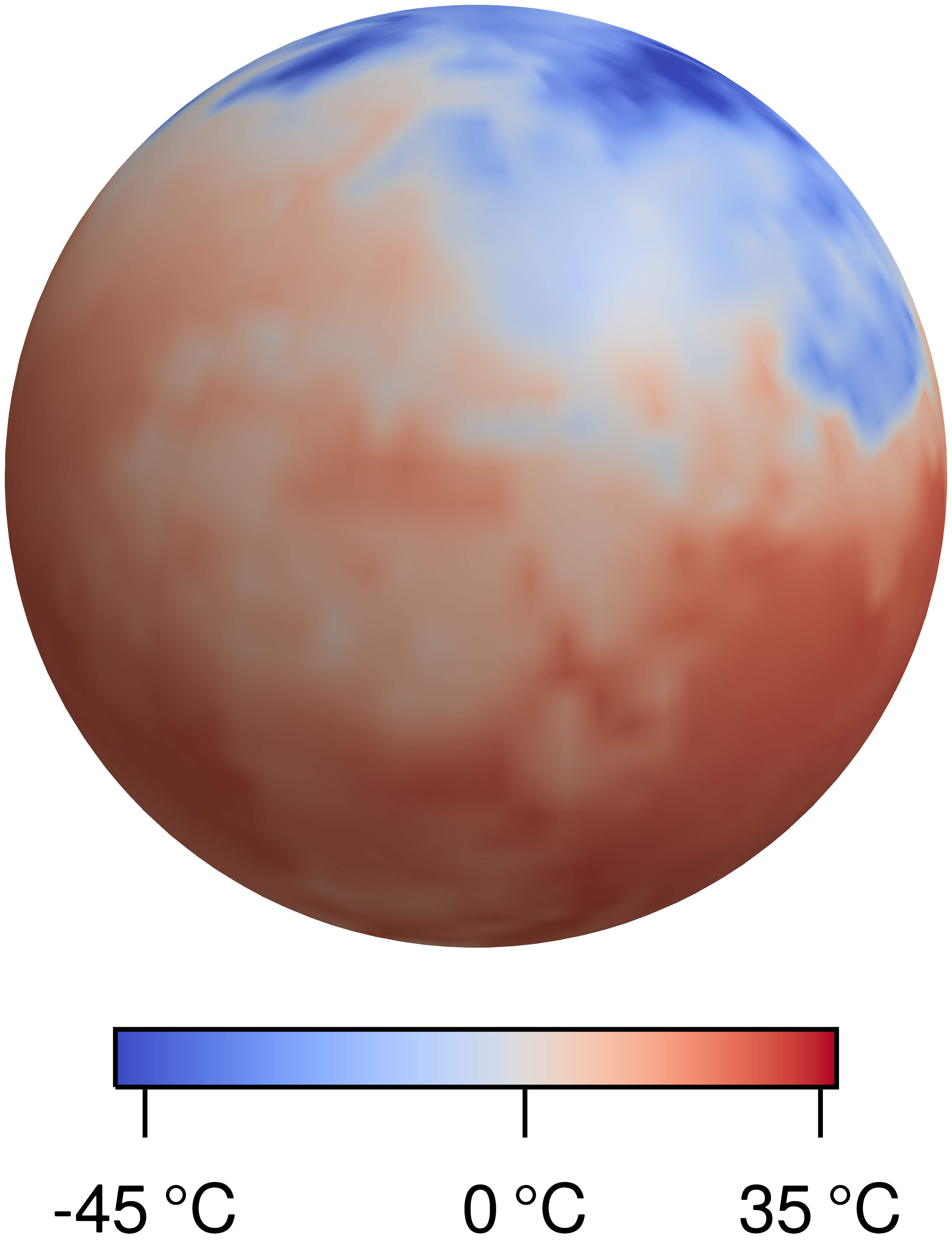
Standard Deviation
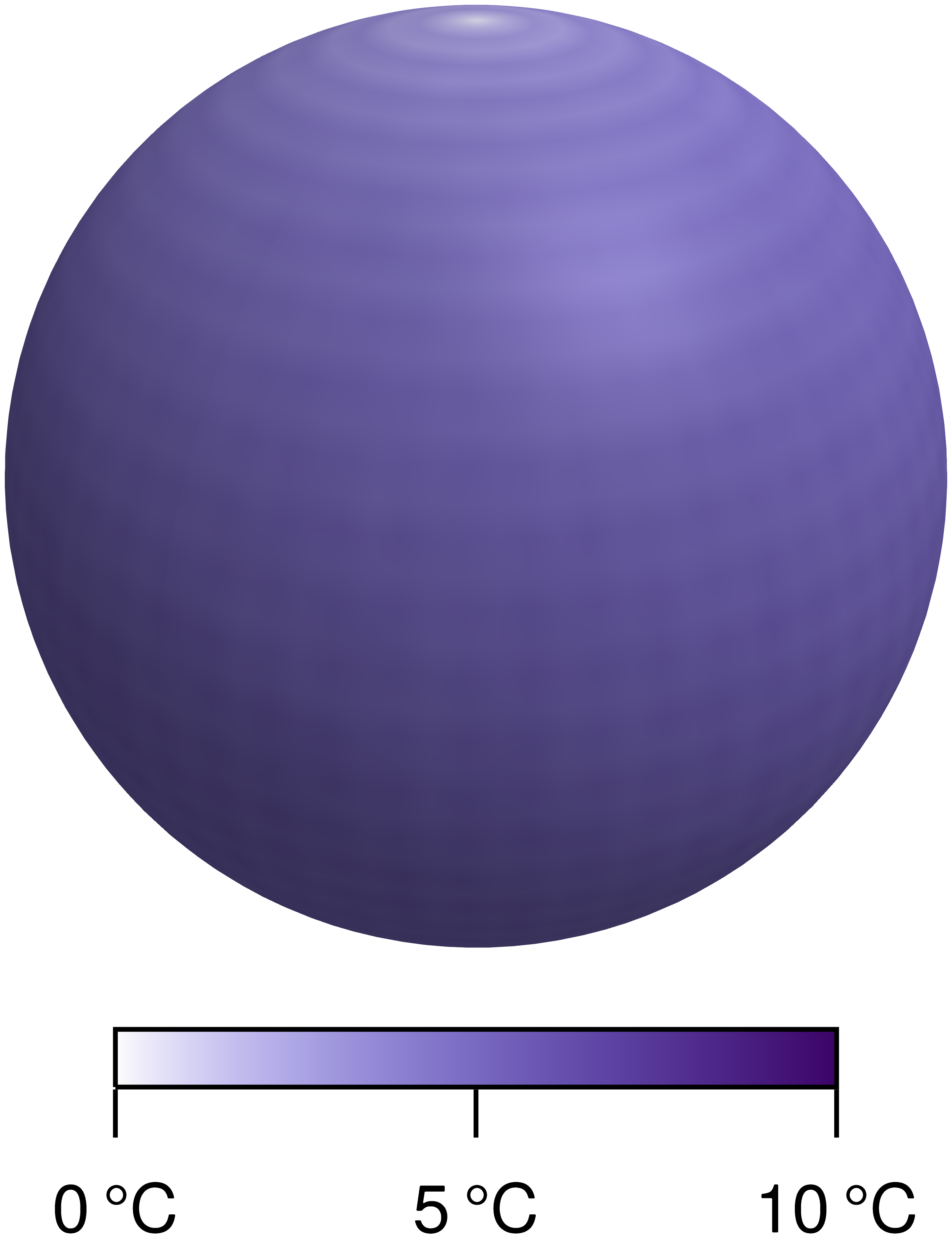
0.48 Mean
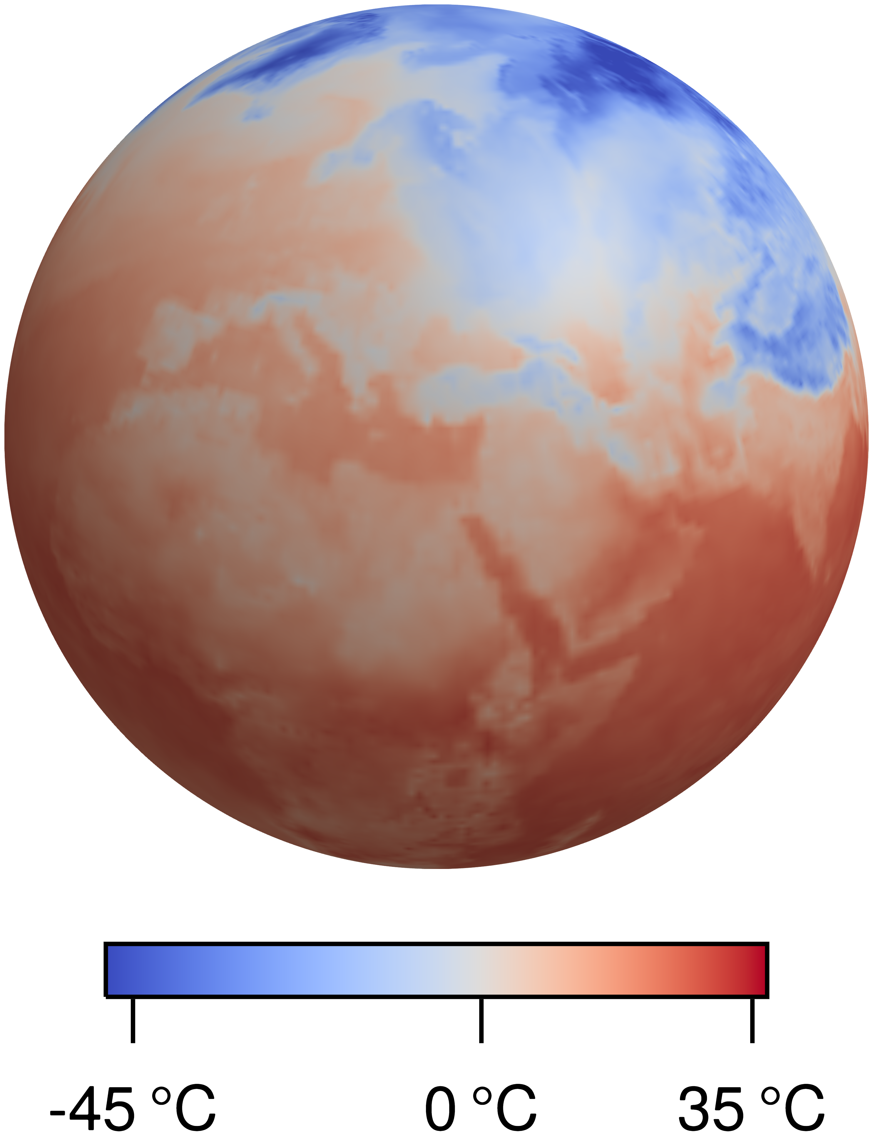
Standard Deviation

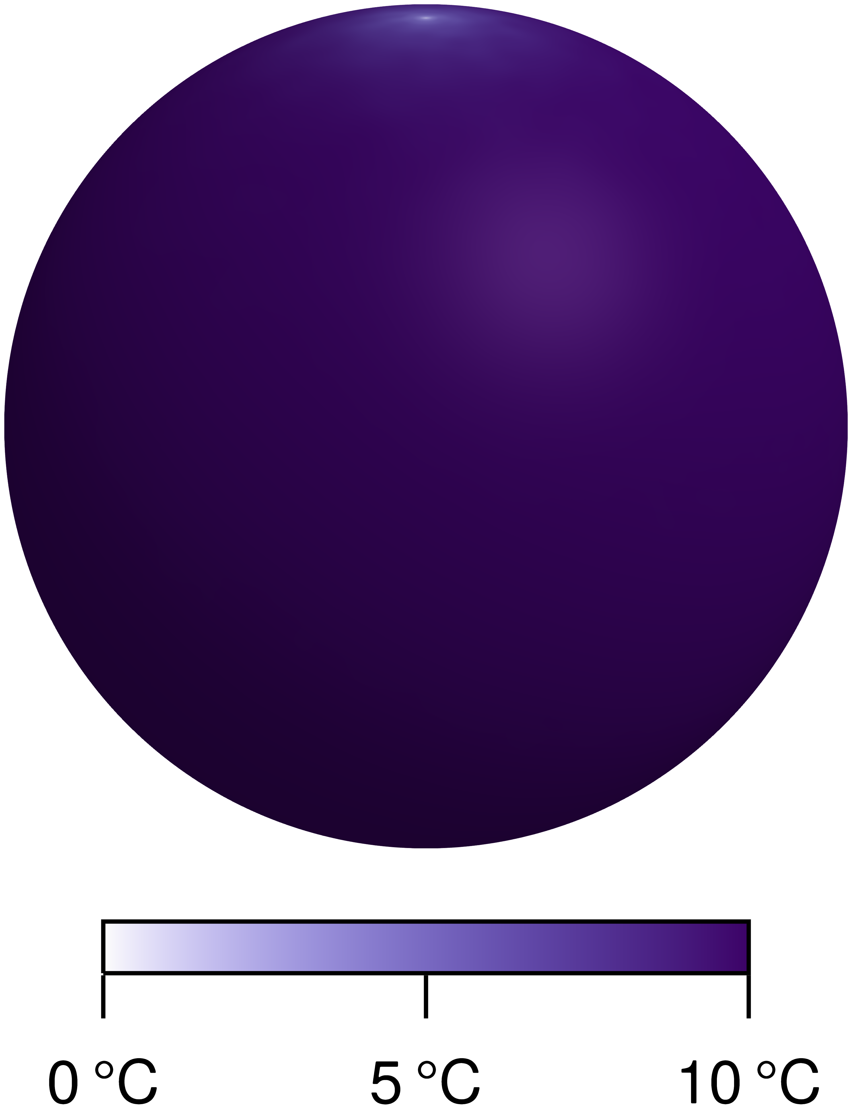
Figure 1: $d=$14\,640$$

Figure 2: $d=$231\,360$$

Figure 3: Spatio-temporal Gaussian process regression of Earth’s surface temperature using the ERA5 dataset [9] via computation-aware filtering and smoothing for two different values of state space dimension $d$. Existing filtering and smoothing methods would require in excess of $\qty{1.17}{\tebi}$ of memory to generate figure 3. Our novel algorithms scale to larger state space dimension $d$ with lower time and memory costs, resolving finer detail and achieving better predictive performance.

Computation-aware Filtering and Smoothing

In this work, we introduce computation-aware Kalman filters (CAKFs) and smoothers (CAKSs): novel approximate versions of the Kalman filter and Rauch-Tung-Striebel (RTS) smoother. Approximations are introduced both to reduce the computational cost through low-dimensional projection of the data (section 3.1) and memory burden through covariance truncation (section 3.2). Alongside their prediction for the underlying dynamics, they return a combined uncertainty estimate quantifying both epistemic uncertainty and the approximation error. We showcase our approach in Figure 3 on a large-scale spatiotemporal regression problem.

Contribution We introduce the CAKF and CAKS, novel filtering and smoothing algorithms that are:

1. iterative and matrix-free, and can fully leverage modern parallel hardware (i.e. GPUs);

2. more efficient both in time and space than their standard versions (see section 6.1); and

3. computation-aware, i.e. they come with theoretical guarantees for their uncertainty estimates which capture the inevitable approximation error (theorem 1).

We demonstrate the scalability of our approach empirically on climate data with up to $n_{t}\cdot n_{\bm{x}}\approx$4$\mathrm{M}$ observations and state space dimension $d\approx 230\mathrm{k}$.

2 Background

Many temporal processes can be modeled with a linear Gaussian state space model, in which exact Bayesian inference can be done efficiently using the Kalman filter and smoother.

2.1 Inference in Linear-Gaussian State Space Models

In the following, we want to infer the values of the states ${\bm{\mathrm{u}}}_{k}$ of an unobserved discrete-time Gauss-Markov process $\{{\bm{\mathrm{u}}}_{k}\}_{k=1}^{n_{t}}$ (or a discretized continuous-time Gauss-Markov process with ${\bm{\mathrm{u}}}_{k}={\bm{\mathrm{u}}}(t_{k})$) defined by the dynamics model

$${\bm{\mathrm{u}}}_{k}={\bm{A}}_{k-1}{\bm{\mathrm{u}}}_{k-1}+{\bm{b}}_{k-1}+{\bm{\mathrm{q}}}_{k-1}\in{\mathbb{R}}^{d}$$

with ${\bm{\mathrm{u}}}_{0}\sim{\operatorname{\mathcal{N}}\left({\bm{\mu}}_{0},{\bm{\Sigma}}_{0}\right)}$ and ${\bm{\mathrm{q}}}_{k-1}\sim{\operatorname{\mathcal{N}}\left({\bm{0}},{\bm{Q}}_{k-1}\right)}$ from a given set of noisy observations $\{{\bm{y}}_{k}\}_{k=1}^{n_{k}}$ made through the observation model

$${\bm{\mathrm{y}}}_{k}={\bm{H}}_{k}{\bm{\mathrm{u}}}_{k}+{\bm{\mathrm{\epsilon}}}_{k}\in{\mathbb{R}}^{n_{k}}.$$

with ${\bm{\mathrm{\epsilon}}}_{k}\sim{\operatorname{\mathcal{N}}\left({\bm{0}},{\bm{\Lambda}}_{k}\right)}$. Collectively, the dynamics and observation models are referred to as a linear-Gaussian state space model (LGSSM). The initial state ${\bm{\mathrm{u}}}_{0}$, the process noise $\{{\bm{\mathrm{q}}}_{k}\}_{k=1}^{n_{t}}$, and the observation noise $\{{\bm{\mathrm{\epsilon}}}_{k}\}_{k=1}^{n_{t}}$ are pairwise independent. One can show that ${\bm{\mathrm{u}}}_{k}\sim{\operatorname{\mathcal{N}}\left({\bm{\mu}}_{k},{\bm{\Sigma}}_{k}\right)}$, where ${\bm{\mu}}_{k+1}\coloneqq{\bm{A}}_{k}{\bm{\mu}}_{k}+{\bm{b}}_{k}$ and ${\bm{\Sigma}}_{k+1}\coloneqq{\bm{A}}_{k}{\bm{\Sigma}}_{k}{\bm{A}}_{k}^{\top}+{\bm{Q}}_{k}$. The Kalman filter is an algorithm for computing conditional distributions of the form ${\bm{\mathrm{u}}}_{k}\nonscript\>|\allowbreak\nonscript\>\mathopen{}{\bm{\mathrm{y}}}_{1:k}={\bm{y}}_{1:k}$, $k=1,\dots,n_{t}$. It alternates recursively between computing the moments

$${\bm{m}}^{-}_{k} \coloneqq{\bm{A}}_{k-1}{\bm{m}}_{k-1}$$

$${\bm{P}}^{-}_{k} \coloneqq{\bm{A}}_{k-1}{\bm{P}}_{k-1}{\bm{A}}_{k-1}^{\top}+{\bm{Q}}_{k-1}$$

of ${\bm{\mathrm{u}}}^{f-}_{k}\coloneqq({\bm{\mathrm{u}}}_{k}\mid{\bm{\mathrm{y}}}_{1:k-1}={\bm{y}}_{1:k-1})\sim{\operatorname{\mathcal{N}}\left({\bm{m}}^{-}_{k},{\bm{P}}^{-}_{k}\right)}$ in the predict step and the moments

$${\bm{m}}_{k} \coloneqq{\bm{m}}^{-}_{k}+{\bm{P}}^{-}_{k}{\bm{H}}_{k}{\bm{G}}_{k}^{-1}({\bm{\mathrm{y}}}_{k}-{\bm{H}}_{k}{\bm{m}}^{-}_{k})$$ (2.1a)

$${\bm{P}}_{k} \coloneqq{\bm{P}}^{-}_{k}-{\bm{P}}^{-}_{k}{\bm{H}}_{k}{\bm{G}}_{k}^{-1}{\bm{H}}_{k}^{\top}{\bm{P}}^{-}_{k}$$ (2.1b)

of ${\bm{\mathrm{u}}}^{f}_{k}\coloneqq({\bm{\mathrm{u}}}_{k}\mid{\bm{\mathrm{y}}}_{1:k}={\bm{y}}_{1:k})\sim{\operatorname{\mathcal{N}}\left({\bm{m}}_{k},{\bm{P}}_{k}\right)}$ in the update step, where ${\bm{G}}_{k}\coloneqq{\bm{H}}_{k}{\bm{P}}^{-}_{k}{\bm{H}}_{k}^{\top}+{\bm{\Lambda}}_{k}$. The conditional distributions computed by the filter are mainly useful for forecasting. For interpolation, we care about the full Bayesian posterior ${\bm{\mathrm{u}}}^{s}_{k}\coloneqq({\bm{\mathrm{u}}}_{k}\nonscript\>|\allowbreak\nonscript\>\mathopen{}{\bm{\mathrm{y}}}_{1:n_{t}}={\bm{y}}_{1:n_{t}})\sim{\operatorname{\mathcal{N}}\left({\bm{m}}^{s}_{k},{\bm{P}}^{s}_{k}\right)}.$ Its moments can be computed from the filter moments via the Rauch-Tung-Striebel (RTS) smoother recursion

$${\bm{m}}^{s}_{k} \coloneqq{\bm{m}}_{k}+{\bm{K}}^{s}_{k}({\bm{m}}^{s}_{k+1}-{\bm{m}}^{-}_{k+1})$$

$${\bm{P}}^{s}_{k} \coloneqq{\bm{P}}_{k}+{\bm{K}}^{s}_{k}({\bm{P}}^{s}_{k+1}-{\bm{P}}^{-}_{k+1})({\bm{K}}^{s}_{k})^{\top}$$

with ${\bm{K}}^{s}_{k}\coloneqq{\bm{P}}_{k}{\bm{A}}_{k}^{\top}({\bm{P}}^{-}_{k+1})^{-1}$, ${\bm{m}}^{s}_{n_{t}}={\bm{m}}_{n_{t}}$, and ${\bm{P}}^{s}_{n_{t}}={\bm{P}}_{n_{t}}$. See Särkkä and Svensson [3] for an in-depth introduction to Kalman filtering and RTS smoothing.

2.2 Spatiotemporal Regression

A major application of state space models is spatiotemporal Gaussian Process (GP) regression [10, 11]. Suppose we aim to learn a function ${\bm{f}}:[t_{0},T]\times{\mathbb{X}}\to{\mathbb{R}}$ from training data $\{(t_{k},{\bm{X}}_{k}),{\bm{y}}_{k}\}_{k=1}^{n_{t}}\subset([t_{0},T]\times{\mathbb{X}}^{n_{\bm{x}}})\times{\mathbb{R}}^{n_{\bm{x}}}$. Given a GP prior ${\mathrm{f}}\sim{\operatorname{\mathcal{GP}}\left(\mu,\Sigma\right)}$, if the multi-output GP ${\bm{\mathrm{f}}}(t,{\bm{x}})\coloneqq(\partial_{t}^{i}{\mathrm{f}}(t,{\bm{x}}))_{i=0}^{d^{\prime}-1}\in{\mathbb{R}}^{d^{\prime}}$ defined by ${\mathrm{f}}$ and $d^{\prime}-1$ of its time derivatives is a space-time separable Gauss-Markov process (STSGMP), then one can construct an equivalent linear Gaussian state space model (see lemma B.2). The resulting state space dimension $d$ scales linearly with the number of spatial observations $n_{\bm{x}}$. Therefore the computational cost of spatiotemporal GP regression can be reduced from $\mathcal{O}(n_{t}^{3}n_{\bm{x}}^{3})$ to $\mathcal{O}(n_{t}n_{\bm{x}}^{3})$ via Bayesian filtering and smoothing.

3 The Computation-Aware Kalman Filter

Figure 4: Probabilistic graphical model for the computation-aware Kalman filter and RTS smoother. Solid arrows and circles define the joint generative model (i.e. the posterior computed by filter and smoother). Dashed arrows visualize the information flow between nodes, with the corresponding “messages” in parentheses.

While filtering and smoothing are efficient in time, they scale prohibitively with the dimension $d$ of the state space. Direct implementations of the Kalman filter incur two major computational challenges that are addressed with the CAKF:

1. The state covariances ${\bm{P}}^{-}_{k},{\bm{P}}_{k}\in{\mathbb{R}}^{d\times d}$ need to be stored in memory, requiring $\mathcal{O}(d^{2})$ space.

2. The inversion of the innovation matrix ${\bm{G}}_{k}\in{\mathbb{R}}^{n_{k}\times n_{k}}$ costs $\mathcal{O}(n_{k}^{3})$ time and $\mathcal{O}(n_{k}^{2})$ space.

Both of these quickly become prohibitive if $d$ and/or $n_{k}$ is large. To mitigate these costs, we apply iterative, matrix-free linear algebra in the Kalman recursion.

3.1 From Matrix-y to Matrix-Free

We start by noting that the Kalman filter’s update step at time $k$ conditions the predictive belief ${\bm{\mathrm{u}}}^{f-}_{k}$ on the observation that ${\bm{\mathrm{y}}}_{k}={\bm{y}}_{k}$. To reduce both the time and memory complexity of the update step, we project both sides of the observation onto a low-dimensional subspace: $\check{{\bm{\mathrm{y}}}}_{k}\coloneqq{\bm{S}}_{k}^{\top}{\bm{\mathrm{y}}}_{k}={\bm{S}}_{k}^{\top}{\bm{y}}_{k}\eqqcolon\check{{\bm{y}}}_{k},$ where ${\bm{S}}_{k}\in{\mathbb{R}}^{n_{k}\times\check{n}_{k}}$ with $\check{n}_{k}\ll n_{k}$. The corresponding modified observation model then reads

$$\check{{\bm{\mathrm{y}}}}_{k}=\underbracket{{\bm{S}}_{k}^{\top}{\bm{H}}_{k}}_{\eqqcolon\check{{\bm{H}}}_{k}}{\bm{\mathrm{u}}}_{k}+\underbracket{{\bm{S}}_{k}^{\top}{\bm{\mathrm{\epsilon}}}_{k}}_{\eqqcolon\check{{\bm{\mathrm{\epsilon}}}}_{k}}\in{\mathbb{R}}^{\check{n}_{k}},$$ (3.1)

where $\check{{\bm{\mathrm{\epsilon}}}}_{k}\sim{\operatorname{\mathcal{N}}\left({\bm{0}},\check{{\bm{\Lambda}}}_{k}\right)}$ with $\check{{\bm{\Lambda}}}_{k}:={\bm{S}}_{k}^{\top}{\bm{\Lambda}}_{k}{\bm{S}}_{k}$. Consequently, the modified filtering equations can be obtained from equation 2.1 by substituting ${\bm{y}}_{k}\mapsto\check{{\bm{y}}}_{k}$, ${\bm{H}}_{k}\mapsto\check{{\bm{H}}}_{k}$ and $\check{{\bm{\Lambda}}}_{k}\mapsto{\bm{S}}_{k}^{\top}{\bm{\Lambda}}_{k}{\bm{S}}_{k}$. The inversion of the innovation matrix $\check{{\bm{G}}}_{k}\in{\mathbb{R}}^{\check{n}\times\check{n}}$ in the projected update step then costs $\mathcal{O}(\check{n}_{k}^{3})$ time and $\mathcal{O}(\check{n}_{k}^{2})$ memory, which solves (C2).

Since ${\bm{S}}_{k}$ is not square the projection results in a loss of information and the filtering moments $\{\hat{{\bm{m}}}_{k},\hat{{\bm{P}}}_{k}\}_{k=1}^{n_{t}}$ and $\{\hat{{\bm{m}}}^{-}_{k},\hat{{\bm{P}}}^{-}_{k}\}_{k=1}^{n_{t}}$ obtained from the Kalman recursion with the modified observation model 3.1 are only approximations of the corresponding moments from the unmodified Kalman recursion. We can choose the columns of ${\bm{S}}_{k}$, the actions, such that they retain the most informative parts of the observation, keeping the approximation error small (more on this in section 3.3). Moreover, we show in section 6 that the approximation error in the state mean will be accounted for by an increase in the corresponding state covariance and hence our inference procedure is computation-aware (in the sense of [12]). In essence, this is because we made the projection onto ${\bm{S}}_{k}$ part of the modified observation model 3.1, i.e. the likelihood accounts for the fact that we do not observe the data ${\bm{y}}_{k}$ in the orthogonal complement of $\operatorname{span}\left({\bm{S}}_{k}\right)$. The resulting posterior is sometimes called a partial posterior, and such posteriors are known to provide sensible uncertainty quantification under certain technical assumptions [13].

Since $\check{n}_{k}\ll n_{k}$, one can show that the updated state covariance $\hat{{\bm{P}}}_{k}$ under the modified observation model differs from the corresponding predictive state covariance $\hat{{\bm{P}}}^{-}_{k}$ by a low-rank downdate

$$\hat{{\bm{P}}}_{k}=\hat{{\bm{P}}}^{-}_{k}-\hat{{\bm{P}}}^{-}_{k}\check{{\bm{H}}}_{k}^{\top}\check{{\bm{V}}}_{k}(\hat{{\bm{P}}}^{-}_{k}\check{{\bm{H}}}_{k}^{\top}\check{{\bm{V}}}_{k})^{\top},$$

where $\check{{\bm{V}}}_{k}\in{\mathbb{R}}^{\check{n}_{k}\times\check{n}_{k}}$ with $\check{{\bm{V}}}_{k}\check{{\bm{V}}}_{k}^{\top}=\check{{\bm{G}}}_{k}^{-1}$. It turns out that the recursion for the state covariances in the Kalman filter is compatible with the low-rank downdate structure. More precisely, in proposition A.3, we show that an alternative recursion for $\hat{{\bm{P}}}^{-}_{k}$ and $\hat{{\bm{P}}}_{k}$ is given by

$$\hat{{\bm{P}}}^{-}_{k} ={\bm{\Sigma}}_{k}-\hat{{\bm{M}}}^{-}_{k}(\hat{{\bm{M}}}^{-}_{k})^{\top},$$ (3.2a)

$$\hat{{\bm{P}}}_{k} ={\bm{\Sigma}}_{k}-\hat{{\bm{M}}}_{k}\hat{{\bm{M}}}_{k}^{\top},$$ (3.2b)

where $\hat{{\bm{M}}}^{-}_{k}={\bm{A}}_{k-1}\hat{{\bm{M}}}_{k-1}$ and $\hat{{\bm{M}}}_{k}=(\hat{{\bm{M}}}^{-}_{k}\ \ \ \hat{{\bm{P}}}^{-}_{k}\check{{\bm{H}}}_{k}^{\top}\check{{\bm{V}}}_{k})$. Incidentally, this observation solves (C1): When implementing the CAKF using the recursions in equation 3.2, we only need access to matrix-vector products ${\bm{\Sigma}}_{k}{\bm{v}}$, ${\bm{A}}_{k}{\bm{v}}$, ${\bm{H}}_{k}^{\top}{\bm{v}}$, and ${\bm{\Lambda}}_{k}{\bm{v}}$ with $\check{n}_{k}+1$ vectors ${\bm{v}}$. In many cases, such matrix-vector products can be efficiently implemented or accurately approximated in a “matrix-free” fashion, i.e. without needing to explicitly store the matrix in memory, at cost less than $\mathcal{O}(d^{2})$ time and (much) less than $\mathcal{O}(d^{2})$ space. For instance, this is possible if $\{{\bm{\mathrm{u}}}_{k}\}_{k=0}^{n_{t}}$ is a discretization of a continuous-time space-time separable Gauss-Markov process with known covariance function, in which case a mathematical expression for the entries $({\bm{\Sigma}}_{k})_{ij}$ of the state covariance is known. We emphasize the matrix-free implementation of our algorithm where matrices are greyed-out or followed by square brackets (i.e. ${\bm{\Sigma}}_{k}[\cdot]$) in algorithms 1, 2, 3 and 4. Assuming the rank of the downdates in equation 3.2 is small (see also section 3.2), such a matrix-free implementation of a Kalman filter only incurs linear memory cost per time step.

Pseudocode for the procedure outlined above can be found in algorithms 1 and 2. In the algorithm, the IsMissing line is included to allow a user to make predictions for intermediate states $k$ for which there is no associated data. The choice of ${\bm{S}}_{k}$ is given by a state-dependent Policy. In algorithm 2 ${\bm{S}}_{k}$ is selected in batch through a single call to Policy at the beginning of each update step. This is mostly presented for clarity; in practice we implement the update step as shown in algorithm A.1. Algorithm A.1 can be derived as successive conditioning of $\hat{{\bm{\mathrm{u}}}}^{f-}_{k}$ on the events $\langle{\bm{s}}_{k}^{(i)},{\bm{\mathrm{y}}}_{k}\rangle_{2}=\langle{\bm{s}}_{k}^{(i)},{\bm{y}}_{k}\rangle_{2}$ for $i=1,\dotsc,\check{n}_{k}$, where the actions ${\bm{s}}_{k}^{(i)}$ form the columns of ${\bm{S}}_{k}$. One can show that this is equivalent to conditioning on ${\bm{S}}_{k}^{\top}{\bm{\mathrm{y}}}_{k}={\bm{S}}_{k}^{\top}{\bm{y}}_{k}$. However, such a sequential selection of the actions through calls to Policy that are allowed to depend on the current state of the iteration (e.g. through data residuals) allows the actions to adapt to the problem more effectively.

Algorithm 1 Computation-Aware Kalman Filter (CAKF)

Filter$\hat{{\bm{m}}}_{0},\{{\bm{\Sigma}}_{k},{\bm{A}}_{k},{\bm{b}}_{k},{\bm{H}}_{k},{\bm{\Lambda}}_{k},{\bm{y}}_{k}\}_{k=1}^{n_{t}}$

$\hat{{\bm{M}}}^{+}_{0}\leftarrow(\quad)\in{\mathbb{R}}^{d\times 0}$ $k=1,\dotsc,n_{t}$

$\phantom{\hat{{\bm{M}}}^{-}_{k}}\mathllap{\hat{{\bm{m}}}^{-}_{k}}\leftarrow{\bm{A}}_{k-1}[\hat{{\bm{m}}}_{k-1}]+{\bm{b}}_{k-1}$ $\triangleright$ Predict

$\hat{{\bm{M}}}^{-}_{k}\leftarrow{\bm{A}}_{k-1}[\hat{{\bm{M}}}^{+}_{k-1}]$ $\neg\Call{IsMissing}{{\bm{y}}_{k}}$

$\hat{{\bm{m}}}_{k},\hat{{\bm{M}}}_{k}\leftarrow\Call{Update}{\hat{{\bm{m}}}^{-}_{k},\hat{{\bm{M}}}^{-}_{k},\dotsc}$

$\hat{{\bm{m}}}_{k},\hat{{\bm{M}}}_{k}\leftarrow\hat{{\bm{m}}}^{-}_{k},\hat{{\bm{M}}}^{-}_{k}$

$\hat{{\bm{M}}}^{+}_{k}\leftarrow\Call{Truncate}{\hat{{\bm{M}}}_{k}}$

return $\{\hat{{\bm{m}}}_{k},\hat{{\bm{M}}}_{k}\}_{k=1}^{n_{t}}$

Algorithm 2 CAKF Update Step

Update$\hat{{\bm{m}}}^{-},\hat{{\bm{M}}}^{-},{\bm{\Sigma}},{\bm{H}},{\bm{\Lambda}},{\bm{y}}$

$\phantom{\check{{\bm{H}}}^{\top}}\mathllap{\hat{{\bm{P}}}^{-}}\leftarrow{\bm{\Sigma}}-\hat{{\bm{M}}}^{-}(\hat{{\bm{M}}}^{-})^{\top}$

$\phantom{\check{{\bm{H}}}^{\top}}\mathllap{{\bm{S}}}\leftarrow\Call{Policy}{\hat{{\bm{m}}}^{-},\hat{{\bm{P}}}^{-},\dotsc}$

$\phantom{\check{{\bm{H}}}^{\top}}\mathllap{\check{{\bm{H}}}^{\top}}\leftarrow{\bm{H}}^{\top}[{\bm{S}}]$

$\phantom{\check{{\bm{H}}}^{\top}}\mathllap{\check{{\bm{\Lambda}}}}\leftarrow{\bm{S}}^{\top}{\bm{\Lambda}}[{\bm{S}}]$

$\phantom{\check{{\bm{H}}}^{\top}}\mathllap{\check{{\bm{y}}}}\leftarrow{\bm{S}}^{\top}{\bm{y}}$

$\phantom{\check{{\bm{H}}}^{\top}}\mathllap{\check{{\bm{G}}}}\leftarrow\check{{\bm{H}}}\hat{{\bm{P}}}^{-}[\check{{\bm{H}}}^{\top}]+\check{{\bm{\Lambda}}}$

$\phantom{\check{{\bm{H}}}^{\top}}\mathllap{\hat{{\bm{w}}}}\leftarrow\check{{\bm{H}}}^{\top}\check{{\bm{G}}}^{\dagger}(\check{{\bm{y}}}-\check{{\bm{H}}}\hat{{\bm{m}}}^{-})$

$\phantom{\check{{\bm{H}}}^{\top}}\mathllap{\hat{{\bm{W}}}}\leftarrow\check{{\bm{H}}}^{\top}(\check{{\bm{G}}}^{\dagger})^{\frac{1}{2}}$

$\phantom{\check{{\bm{H}}}^{\top}}\mathllap{\hat{{\bm{m}}}}\leftarrow\hat{{\bm{m}}}^{-}+\hat{{\bm{P}}}^{-}[\hat{{\bm{w}}}]$

$\phantom{\check{{\bm{H}}}^{\top}}\mathllap{\hat{{\bm{M}}}}\leftarrow\begin{pmatrix}\hat{{\bm{M}}}^{-}&\hat{{\bm{P}}}^{-}[\hat{{\bm{W}}}]\end{pmatrix}$

return $(\hat{{\bm{m}}},\hat{{\bm{M}}})$

3.2 Downdate Truncation

While the algorithm is matrix-free in the sense of not needing to compute and store $d\times d$ matrices, the accumulation of the downdate matrices $\hat{{\bm{M}}}_{k}$ results in an $\mathcal{O}(d\sum_{l=1}^{k}\check{n}_{l})$ memory cost at step $k$, which can easily exceed $\mathcal{O}(d^{2})$. To address this, in this section we introduce an optimal truncation of the downdate matrices in the Truncate procedure to control the memory requirements of the algorithm.

Consider the square root $\hat{{\bm{M}}}_{k}\in{\mathbb{R}}^{d\times r_{k}}$ of a belief covariance downdate. To truncate the downdate matrices we fix a maximal rank $r^{\text{max}}_{k}$. Then at each iteration we select $r^{+}_{k}=\min(r_{k},r^{\text{max}}_{k})$, $\hat{{\bm{M}}}^{+}_{k}\in{\mathbb{R}}^{d\times r^{+}_{k}}$, and ${\bm{N}}_{k}\in{\mathbb{R}}^{d\times(r_{k}-r^{+}_{k})}$ such that $\hat{{\bm{M}}}_{k}\hat{{\bm{M}}}_{k}^{\top}=\hat{{\bm{M}}}^{+}_{k}(\hat{{\bm{M}}}^{+}_{k})^{\top}+{\bm{N}}_{k}{\bm{N}}_{k}^{\top}$ and approximate $\hat{{\bm{M}}}_{k}\approx\hat{{\bm{M}}}^{+}_{k}$ as well as $\hat{{\bm{P}}}_{k}\approx\hat{{\bm{P}}}^{+}_{k}\coloneqq{\bm{\Sigma}}_{k}-\hat{{\bm{M}}}^{+}_{k}(\hat{{\bm{M}}}^{+}_{k})^{\top}.$ Noting that $\hat{{\bm{P}}}^{+}_{k}=\hat{{\bm{P}}}_{k}+{\bm{N}}_{k}{\bm{N}}_{k}^{\top}$, we realise that the truncation of the downdate can be interpreted as the addition of independent computational uncertainty [12]: additional noise ${\bm{\mathrm{q}}}^{\text{comp}}_{k}\sim{\operatorname{\mathcal{N}}\left({\bm{0}},{\bm{N}}_{k}{\bm{N}}_{k}^{\top}\right)}$ added to the posterior covariance to account for uncertainty due to incomplete computation, in this case, truncation. To represent the addition of computational uncertainty due to truncation, we augment the dynamics model with additional prior states ${\bm{\mathrm{u}}}^{+}_{k},{\bm{\mathrm{u}}}^{-}_{k}$ as visualized in figure 4, such that

$${\bm{\mathrm{u}}}^{+}_{k} \coloneqq{\bm{\mathrm{u}}}_{k}+{\bm{\mathrm{q}}}^{\text{comp}}_{k}$$

$${\bm{\mathrm{u}}}^{-}_{k+1} \coloneqq{\bm{A}}_{k}{\bm{\mathrm{u}}}^{+}_{k}+{\bm{b}}_{k}+{\bm{\mathrm{q}}}_{k}$$

$${\bm{\mathrm{u}}}_{k} \coloneqq{\bm{\mathrm{u}}}^{-}_{k+1}$$

Even though the truncation leads to a further approximation of the state beliefs, this approximation will be conservative, which directly follows from the computational noise interpretation above.

We truncate by computing a singular-value decomposition of $\hat{{\bm{M}}}_{k}\hat{{\bm{M}}}_{k}^{\top}$, and dropping the subspace corresponding to the smallest singular vectors. By the Eckart-Young-Mirsky theorem [14], this truncation is optimal with respect to all unitarily invariant matrix norms. The effect of rank truncation is that at most $\mathcal{O}(dr_{k}^{+})$ memory is required to store the downdate matrices, and that the cost of computing matrix-vector products with the truncated covariance $\hat{{\bm{P}}}^{+}_{k}$ is at most $\mathcal{O}(\rho_{k}+dr_{k}^{+})$, where $\rho_{k}$ is the cost of computing a matrix-vector product with ${\bm{\Sigma}}_{k}$.

3.3 Choice of Policy

It remains to specify a Policy defining the actions ${\bm{S}}_{k}$. This can have a significant impact on the algorithm, both from the perspective of how close the CAKF states are to the states of the true Kalman filter and in terms of its computational cost. Heuristically we would like to make $\check{n}_{k}$ as small as possible while keeping $\hat{{\bm{\mathrm{u}}}}^{f}_{k}$ close to ${\bm{\mathrm{u}}}^{f}_{k}$. We discuss and compare a number of natural policy choices in more detail in Section C.2. In the experiments in section 8 we exclusively use Lanczos/CG-based directions, corresponding to choosing the current residual $\smash{\hat{{\bm{r}}}_{k}^{(i)}}$ as the action in iteration $i$ of algorithm A.1, i.e. $\textsc{Policy}(i,\dotsc)=\smash{\hat{{\bm{r}}}_{k}^{(i)}}$. We found these to perform well empirically compared to other choices (see Figure C.1), and similar policies have been found effective for other applications of probabilistic linear solvers [15, 12].

4 Computation-Aware RTS Smoothing

If the state space dimension $d$ is large, naive implementations of the RTS smoother face similar challenges to those outlined for the Kalman filter in section 3. This is due to the smoother gain matrices ${\bm{K}}^{s}_{k}$ needing to be stored and inverted at $\mathcal{O}(d^{3})$ time and $\mathcal{O}(d^{2})$ memory cost. Fortunately, we can apply a similar strategy to section 3.1 to make the smoother matrix-free. Specifically, in proposition A.5 we show that the mean and covariance of the RTS smoother can be computed from quantities precomputed in the Kalman filter, i.e. without the need to compute any additional inverses:

$${\bm{m}}^{s}_{k} ={\bm{m}}_{k}+{\bm{P}}_{k}{\bm{A}}_{k}^{\top}{\bm{w}}^{s}_{k}$$

$${\bm{P}}^{s}_{k} ={\bm{\Sigma}}_{k}-{\bm{M}}^{s}_{k}({\bm{M}}^{s}_{k})^{\top}$$

with ${\bm{M}}^{s}_{k}=\begin{pmatrix}{\bm{M}}_{k}&{\bm{P}}_{k}{\bm{A}}_{k}^{\top}{\bm{W}}^{s}_{k}\end{pmatrix}$ where recursive expressions for ${\bm{w}}^{s}_{k}$ and ${\bm{W}}^{s}_{k}$ are given in equations A.1 and A.2. Hence, just as for the filtering covariances, the smoother covariances take the form of a downdated prior covariance. The terms ${\bm{w}}^{s}_{k}$ and ${\bm{W}}^{s}_{k}$ can be efficiently computed from quantities cached in algorithms 1 and 2 without materializing any $\mathcal{O}(d^{2})$ matrices in memory. Applying proposition A.5 in matrix-free form to the modified state space model of the CAKF introduced in section 3 yields algorithm 3 – the computation-aware RTS smoother (CAKS).

Algorithm 3 Computation-Aware RTS Smoother (CAKS)

Smooth$\{\dotsc,\hat{{\bm{m}}}_{k},\hat{{\bm{M}}}_{k},\hat{{\bm{w}}}_{k},\hat{{\bm{W}}}_{k},\dotsc\}_{k=1}^{n_{t}}$

$\phantom{\hat{{\bm{W}}}^{s}_{n_{t}}}\mathllap{\hat{{\bm{w}}}^{s}_{n_{t}}}\leftarrow\hat{{\bm{w}}}_{n_{t}}$

$\hat{{\bm{W}}}^{s}_{n_{t}}\leftarrow\hat{{\bm{W}}}_{n_{t}}$ $k=n_{t}-1,\dotsc,1$

$\phantom{\hat{{\bm{W}}}^{s}_{n_{t}}}\mathllap{\hat{{\bm{m}}}^{s}_{k}}\leftarrow\hat{{\bm{m}}}_{k}+\hat{{\bm{P}}}_{k}[{\bm{A}}_{k}^{\top}\hat{{\bm{w}}}^{s}_{k+1}]$

$\phantom{\hat{{\bm{W}}}^{s}_{n_{t}}}\mathllap{\hat{{\bm{M}}}^{s}_{k}}\leftarrow\begin{pmatrix}\hat{{\bm{M}}}_{k}&\hat{{\bm{P}}}_{k}[{\bm{A}}_{k}^{\top}\hat{{\bm{W}}}^{s}_{k+1}]\end{pmatrix}$

$\phantom{\hat{{\bm{W}}}^{s}_{n_{t}}}\mathllap{\hat{{\bm{P}}}^{-}_{k}}\leftarrow{\bm{\Sigma}}_{k}-\hat{{\bm{M}}}^{-}_{k}(\hat{{\bm{M}}}^{-}_{k})^{\top}\in{\mathbb{R}}^{d\times d}$

$\phantom{\hat{{\bm{W}}}^{s}_{n_{t}}}\mathllap{\hat{{\bm{w}}}^{s}_{k}}\leftarrow\hat{{\bm{w}}}_{k}+({\bm{I}}-\hat{{\bm{W}}}_{k}\hat{{\bm{W}}}_{k}^{\top}\hat{{\bm{P}}}^{-}_{k})[{\bm{A}}_{k}^{\top}\hat{{\bm{w}}}^{s}_{k+1}]$

$\phantom{\hat{{\bm{W}}}^{s}_{n_{t}}}\mathllap{\hat{{\bm{W}}}^{s}_{k}}\leftarrow\begin{pmatrix}\hat{{\bm{W}}}_{k}&({\bm{I}}-\hat{{\bm{W}}}_{k}\hat{{\bm{W}}}_{k}^{\top}\hat{{\bm{P}}}^{-}_{k})[{\bm{A}}_{k}^{\top}\hat{{\bm{W}}}^{s}_{k+1}]\end{pmatrix}$

$\phantom{\hat{{\bm{W}}}^{s}_{n_{t}}}\mathllap{\hat{{\bm{W}}}^{s}_{k}}\leftarrow\Call{Truncate}{\hat{{\bm{W}}}^{s}_{k}}$

return $\{\hat{{\bm{m}}}^{s}_{k},\hat{{\bm{M}}}^{s}_{k}\}_{k=1}^{n_{t}}$

Algorithm 4 CAKF/CAKS Sampler

Sample$\{\cdots,\hat{{\bm{M}}}_{k},\hat{{\bm{V}}}_{k},\hat{{\bm{W}}}_{k},\dotsc\}_{k=1}^{n_{t}}$

1:$\hat{{\bm{\mathrm{u}}}}^{f}_{0}\sim{\operatorname{\mathcal{N}}\left({\bm{\mu}}_{0},{\bm{\Sigma}}_{0}\right)}$ $k=1,\dotsc,n_{t}$

2:$\phantom{\hat{{\bm{\mathrm{u}}}}^{f-}_{k}}\mathllap{{\bm{\mathrm{q}}}_{k-1}}\sim{\operatorname{\mathcal{N}}\left({\bm{0}},{\bm{Q}}_{k-1}\right)}$

3:$\phantom{\hat{{\bm{\mathrm{u}}}}^{f-}_{k}}\mathllap{{\bm{\mathrm{\epsilon}}}_{k}}\sim{\operatorname{\mathcal{N}}\left({\bm{0}},{\bm{\Lambda}}_{k}\right)}$

4:$\phantom{\hat{{\bm{\mathrm{u}}}}^{f-}_{k}}\mathllap{\hat{{\bm{\mathrm{u}}}}^{f-}_{k}}\leftarrow{\bm{A}}_{k-1}\hat{{\bm{\mathrm{u}}}}^{f}_{k-1}+{\bm{b}}_{k-1}+{\bm{\mathrm{q}}}_{k-1}$

5:$\phantom{\hat{{\bm{\mathrm{u}}}}^{f-}_{k}}\mathllap{\hat{{\bm{\mathrm{w}}}}_{k}}\leftarrow\hat{{\bm{W}}}_{k}\hat{{\bm{V}}}_{k}^{\top}[{\bm{y}}_{k}-{\bm{H}}_{k}\hat{{\bm{\mathrm{u}}}}^{f-}_{k}-{\bm{\mathrm{\epsilon}}}_{k}]$

6:$\phantom{\hat{{\bm{\mathrm{u}}}}^{f-}_{k}}\mathllap{\hat{{\bm{\mathrm{u}}}}^{f}_{k}}\leftarrow\hat{{\bm{\mathrm{u}}}}^{f-}_{k}+\hat{{\bm{P}}}^{-}_{k}[\hat{{\bm{\mathrm{w}}}}_{k}]$

7:$\hat{{\bm{\mathrm{w}}}}^{s}_{n}=\hat{{\bm{\mathrm{w}}}}_{n_{t}}$ $k=n_{t}-1,\dotsc,1$

8:$\begin{aligned} \hat{{\bm{\mathrm{w}}}}^{s}_{k}&\leftarrow\hat{{\bm{\mathrm{w}}}}_{k}+{\bm{A}}_{k}[\hat{{\bm{\mathrm{w}}}}^{s}_{k+1}]\\ &\qquad-\hat{{\bm{W}}}_{k}\hat{{\bm{W}}}_{k}^{\top}\hat{{\bm{P}}}^{-}_{k}{\bm{A}}_{k}[\hat{{\bm{\mathrm{w}}}}^{s}_{k+1}]\end{aligned}$

9:return $\{\hat{{\bm{\mathrm{u}}}}^{s}_{k}=\hat{{\bm{\mathrm{u}}}}^{f}_{k}+\hat{{\bm{P}}}_{k}{\bm{A}}_{k}^{\top}[\hat{{\bm{\mathrm{w}}}}^{s}_{k}]\}_{k=1}^{n_{t}}$

While the cost of filtering is reduced by the low-dimensional projection of the data, the same does not hold for the smoother. Examining algorithm 2 we see that $\hat{{\bm{P}}}^{-}_{k}$ only appears in a product with $\check{{\bm{H}}}$, whereas in algorithm 3 products with $\hat{{\bm{P}}}^{-}_{k}$ appear directly. We also note that it is necessary to truncate the directions $\hat{{\bm{W}}}^{s}_{k}$ accumulated over the course of the smoother to mitigate a further $\mathcal{O}(d\sum_{l=k}^{n_{t}}\check{n}_{l})$ storage cost. This is implemented using the same procedure as described in section 3.2.

5 Sampling via Matheron’s Rule

The naive approach to sampling from a multivariate normal distribution (e.g. by Cholesky factorization) has $\mathcal{O}(d^{3})$ cost and requires storing ${\bm{P}}$ in memory, which is not possible for large state space dimension $d$. We alleviate this by employing Matheron’s rule [16], making it possible to sample the filtering and smoothing posteriors by transforming samples from the prior.

To proceed, we assume that it is feasible to obtain an (approximate) sample ${\bm{\mathrm{u}}}_{0}\sim{\operatorname{\mathcal{N}}\left({\bm{\mu}}_{0},{\bm{\Sigma}}_{0}\right)}$, as well as (approximate) samples from the dynamics and observational noise ${\bm{\mathrm{q}}}_{k-1}\sim{\operatorname{\mathcal{N}}\left({\bm{0}},{\bm{Q}}_{k-1}\right)}$, ${\bm{\mathrm{\epsilon}}}_{k}\sim{\operatorname{\mathcal{N}}\left({\bm{0}},{\bm{\Lambda}}_{k}\right)}$, $k=1,\dots,n_{t}$. This assumption is reasonable because the covariance matrices ${\bm{\Sigma}}_{0},{\bm{Q}}_{k-1},{\bm{\Lambda}}_{k}$ are often simple or highly structured; for example it is common for ${\bm{\Lambda}}_{k}$ to be diagonal. Moreover, for discretized spatiotemporal Gauss-Markov processes one can use function space approximations like random Fourier features (RFF) [17] to obtain approximate samples from ${\bm{\mathrm{u}}}_{0}$ and ${\bm{\mathrm{q}}}_{k-1}$ [see also 18]. Finally, Krylov methods can be used to approximate matrix square roots of the covariances in a matrix-free fashion [see e.g. 19]. With these samples, theorem A.6 shows how Matheron sampling can be implemented for the standard Kalman filter and RTS smoother, while proposition A.7 gives an equivalent form of Matheron sampling for the smoother that circumvents inversion of state covariance matrices.

Each of these approaches can be applied to the modified state space model used in the CAKF and the CAKS at low cost, again recycling computed values from the filtering pass in algorithms 1 and 2. The resulting algorithm for sampling from the computation-aware posterior process $\{\hat{{\bm{\mathrm{u}}}}^{s}_{k}\}_{k=1}^{n_{t}}$ is detailed in algorithm 4. If it is stopped early before 7, then it can also be used to compute samples from the CAKF states $\{\hat{{\bm{\mathrm{u}}}}^{f}_{k}\}_{k=1}^{n_{t}}$. Also note that algorithm 4 allows us to sample from the full Bayesian posterior without running the CAKS, since all quantities used above have already been computed by the filter.

6 Theoretical Analysis

6.1 Computational Complexity

As mentioned in section 3, the CAKF and CAKS assume that we can efficiently evaluate matrix-vector products with ${\bm{\Sigma}}_{k}$, ${\bm{A}}_{k}$, ${\bm{H}}_{k}^{\top}$, and ${\bm{\Lambda}}_{k}$, without synthesizing the matrices in memory. More precisely, we assume that matrix-vector products with these matrices can be computed with a memory complexity linear in the larger of their two dimensions and with the same worst-case time complexity.

Filtering The CAKF predict step at time $k$ costs at most $\mathcal{O}(d^{2}r^{\text{max}}_{k-1})$ time and $\mathcal{O}(dr^{\text{max}}_{k-1})$ memory. The CAKF update step at time $k$ costs at most $\mathcal{O}\big{(}(dn_{k}+n_{k}^{2}+d^{2})\check{n}_{k}\big{)}$ time and $\mathcal{O}\big{(}(n_{k}+d)\check{n}_{k}\big{)}$ memory. The SVD downdate truncation has a time complexity of at most $\mathcal{O}(d(r^{\text{max}}_{k-1}+\check{n}_{k})^{2})$.

Smoothing CAKS iteration $k$ costs $\mathcal{O}\big{(}d(d+\check{n}_{k})r^{\text{max}}_{k+1}+d\check{n}_{k}^{2}\big{)}$ time and $\mathcal{O}\big{(}(d+\check{n}_{k})r^{\text{max}}_{k+1}\big{)}$ memory.

Simplified Complexities In practice, especially for spatiotemporal GP regression, it virtually always holds that $d=\mathcal{O}(n_{k})$. With this assumption, the time and memory complexities of the CAKF update step simplify to $\mathcal{O}(d^{2}\check{n})$ and $\mathcal{O}(d\check{n})$, respectively. Similarly, iteration $k$ of the smoother then costs $\mathcal{O}(d^{2}(r^{\text{max}}_{k+1}+\check{n}_{k}))$ time and $\mathcal{O}(dr^{\text{max}}_{k+1})$ memory. It is also sometimes desirable to set $r^{\text{max}}_{k}=r^{\text{max}}$ and $\check{n}_{k}=\check{n}$, i.e. uniform in $k$, with $r^{\text{max}}=\mathcal{O}(\check{n})$. In this case, running both CAKF and CAKS for $n_{t}$ time steps results in worst-case time and memory complexities of $\mathcal{O}\big{(}n_{t}d^{2}\check{n}\big{)}$ and $\mathcal{O}\big{(}n_{t}d\check{n}\big{)}$.

6.2 Error Bound for Spatiotemporal Regression

From a theoretical perspective, it is important to understand the impact of the approximations made by the CAKF and CAKS on the resulting predictions. So far we have argued informally, that the additional uncertainty of the CAKS captures the approximation error. We will now make this statement rigorous for the case of spatiotemporal regression.

Theorem 1 (Pointwise Worst-Case Prediction Error).

Let ${\mathbb{Z}}=[t_{0},T]\times{\mathbb{X}}$ and define a space-time separable Gauss-Markov process ${\bm{\mathrm{f}}}\sim{\operatorname{\mathcal{GP}}\left({\bm{\mu}},{\bm{\Sigma}}\right)}$ such that its first component ${\mathrm{f}}\coloneqq{\mathrm{f}}_{0}\sim{\operatorname{\mathcal{GP}}\left(\mu,\Sigma\right)}$ defines a prior for the latent function $f\in{\mathbb{H}}_{\Sigma}$ generating the data, which is assumed to be an element of the RKHS defined by ${\mathbb{H}}_{\Sigma}$. Given observation noise $\sigma^{2}\geq 0$, let $y(\cdot)\in{\mathbb{H}}_{\Sigma^{\sigma}}$ be the observed process with $\Sigma^{\sigma}({\bm{z}},{\bm{z}}^{\prime})\coloneqq\Sigma({\bm{z}},{\bm{z}}^{\prime})+\sigma^{2}\delta({\bm{z}},{\bm{z}}^{\prime})$. Given training inputs ${{\bm{Z}}_{\text{train}}}\subset{\mathbb{Z}}$ and targets ${\bm{y}}=y({{\bm{Z}}_{\text{train}}})$, let $\hat{\mu}^{y}({\bm{z}})$ and $\hat{\Sigma}({\bm{z}},{\bm{z}})$ be the mean and variance of the CAKS for an arbitrary test input ${\bm{z}}=(t,{\bm{x}})\in{\mathbb{Z}}\setminus{\bm{Z}}$. Then it holds that

$$\sup\limits_{y\in{\mathbb{H}}_{\Sigma^{\sigma}}\setminus\{0\}}\frac{\lvert y({\bm{z}})-\hat{\mu}^{y}({\bm{z}})\rvert}{\lVert y\rVert_{{\mathbb{H}}_{\Sigma^{\sigma}}}}=\sqrt{\hat{\Sigma}({\bm{z}},{\bm{z}})+\sigma^{2}}.$$ (6.1)

If $\sigma^{2}=0$, the above also holds for training inputs ${\bm{z}}\in{{\bm{Z}}_{\text{train}}}$. If ${\bm{z}}=(t,{\bm{x}})$ such that $t\geq t_{n_{t}}$, then it suffices to run the CAKF to compute the mean and variance.

The proof can be found in section B.2. Theorem 1 says that the (relative) worst-case error of the CAKS’s posterior mean $\hat{\mu}^{y}$ computed for data from the data-generating process $y(\cdot)$ is tightly bounded by its predictive standard deviation $(\hat{\Sigma}({\bm{z}},{\bm{z}})+\sigma^{2})^{\nicefrac{{1}}{{2}}}$ (assuming no truncation). Importantly, this guarantee is of the same form as the one satisfied by the exact posterior predictive ${\operatorname{\mathcal{GP}}\left(\bar{\mu}^{y},\bar{\Sigma}^{y}+\sigma^{2}\delta\right)}$ for the same prior (see Prop. 3.8 of Kanagawa et al. [20]), except for the corresponding approximations. In this sense, Theorem 1 makes the nomenclature computation-aware rigorous, since both the error due to finite data and the inevitable approximation error incurred by using $\hat{\mu}^{y}\approx\bar{\mu}^{y}$ for prediction is quantified by its uncertainty estimate. Finally, truncation only increases the marginal variance of the CAKS, which leads us to conject that the same guarantee as in equation 6.1 holds with inequality for truncation.

7 Related Work

Reducing the cost of Kalman filtering and smoothing in the high-dimensional regime is a fundamental problem. A large family of methods accelerates Kalman filtering by truncating state covariance matrices. This includes the ensemble Kalman filter (EnKF) [5] and its many variants as well as the reduced-rank Kalman filter (RRKF) [8]. However in contrast to this work, the above cited papers truncate the full state covariance rather than downdates, which can lead to overconfident uncertainty estimates [8, Appendix E]. Some authors also propose dimension reduction techniques for the state space [e.g. 21] with the notable exception of Berberidis and Giannakis [7], which focuses on data dimension reduction, as we do here. Bardsley et al. [6] uses a similar Lanczos-inspired methodology; in certain settings, this is equivalent to low-dimensional projections of the data.

The main application of high-dimensional filtering and smoothing considered in sections 6 and 8 is to spatiotemporal Gaussian process regression. The connection between this and Bayesian filtering and smoothing was first expounded in Hartikainen and Särkkä [10], Särkkä et al. [11] and generalized to a wider class of covariance functions in Todescato et al. [22]. The works above focus on discretizing the Gaussian process to obtain a state space model. One can also apply the Kalman filter directly in the infinite-dimensional setting, as proposed by Särkkä and Hartikainen [23], Solin and Särkkä [24].

The CAKF is a probabilistic numerical method [25, 26, 27]. In particular, algorithm A.1 is closely related to the literature on probabilistic linear solvers [28, 15, 29], which frequently employ the Lanczos process. The idea of using such solvers for GP regression was explored in Wenger et al. [12], which first proposed the construction of computation-aware solvers; the sense in which the CAKF is computation-aware is slightly different, in that the truncation of the covariance downdates also plays a role. Tatzel et al. [30] explores similar ideas in the context of Bayesian generalized linear models.

8 Experiments

We will now demonstrate the features of the computation-aware Kalman filter and smoother by applying it both to a task with synthetic data and to a large-scale spatiotemporal regression problem.

Implementation A flexible and efficient implementation of the CAKF and CAKS, including Matheron sampling and support for spatiotemporal modeling, is available as an open-source Julia library at https://github.com/marvinpfoertner/ComputationAwareKalman.jl. When applying the CAKF and CAKS to separable spatiotemporal Gauss-Markov models, the main performance bottleneck is the computation of matrix-vector products with the prior’s state covariance, since this involves a multiplication with a large kernel Gram matrix $\Sigma^{\bm{x}}({\bm{X}},{\bm{X}})$. Our Julia implementation includes a custom CUDA kernel for multiplying with Gramians generated by covariance kernels without materializing the matrix in memory.

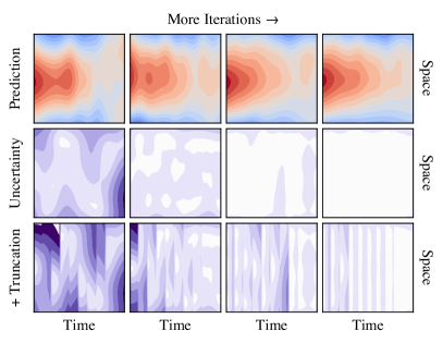
Figure 5: Predictive mean, uncertainty and truncated uncertainty for an increasing number of iterations $\check{n}\equiv\check{n}_{k}$ per time step on a synthetic spatiotemporal regression problem.

8.1 Synthetic Dataset

We generate synthetic data from the latent function $f(t,x)\coloneqq\sin(x)\exp(-t)$ such that ${\mathrm{y}}\sim{\operatorname{\mathcal{N}}\left(f(t,x),\sigma^{2}\right)}$ with $\sigma=0.1$ and define a space-time separable GP prior, which for inference we translate into an equivalent STSGMP (see Section C.1.1 for details). We illustrate the effect of the number of iterations $\check{n}_{k}$ and the truncation rank $r^{\text{max}}_{k}=2\check{n}_{k}$ on the predictive mean and uncertainty in Figure 5. Notice how for an increasing number of iterations the posterior mean $\hat{\mu}$ improves and the posterior variance $\hat{\Sigma}$ reduces. When the belief is (optimally) truncated to save memory, the uncertainty per timestep increases in a structured fashion.

8.2 Climate Dataset

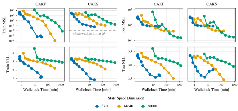
Figure 6: Work-precision diagrams for the CAKF and CAKS on the ERA5 climate dataset. The plot shows the mean squared error (MSE) and negative log-likelihood (NLL) of the computation-aware filter and smoother for different problem sizes (i.e. state space dimension) and number of iterations on the train and test set. The predictive error measured by MSE decreases with larger problem sizes, while the NLL increases. This is because we assume a limited computational budget and thus run fewer iterations for larger problems, i.e. we trade reduced computation cost for increased uncertainty.

To demonstrate that our approach scales to large, real-world problems, we use the CAKS to interpolate earth surface temperature data over time using an STSGMP prior on the sphere.

Data We consider the 2m temperature variable from the ERA5 global reanalysis dataset [9]. The data reside on a 1440$\times$721 spatial latitude-longitude grid with an hourly temporal resolution. For our experiments, we selected the first $\qty{48}{}$ of 2022 with a temporal stride of $\qty{1}{}$, i.e. $n_{t}=48$. To show the effect of different problem sizes on our algorithms, we downsample the dataset by factors of 3, 6, 12, and 24 along both spatial dimensions using nearest neighbor downsampling. A regular subgrid consisting of 25 of the points in the downsampled dataset is used for testing, while the remaining points are used as a training set. The total number of spatial points and the number of spatial training points for each downsampled version of the dataset can be found in table C.1.

Model We choose a zero-mean Gaussian Process prior with a space-time separable covariance function $\Sigma({\bm{z}},{\bm{z}}^{\prime})=\Sigma^{t}(t,t^{\prime})\Sigma^{\bm{x}}({\bm{x}},{\bm{x}}^{\prime})$, where $\Sigma^{t}$ is a Matérn($\nicefrac{{3}}{{2}}$) covariance function and $\Sigma^{\bm{x}}$ is an extrinsic Matérn($\nicefrac{{3}}{{2}}$) kernel on the sphere, i.e. a covariance function on ${\mathbb{R}}^{3}$ concatenated with a coordinate transformation from spherical/geographic coordinates to ${\mathbb{R}}^{3}$ in both arguments. We choose a temporal lengthscale of 3, the spatial lengthscale is set to the geodesic distance of the training points at the equator, and the output scale is 10. We assume the data is corrupted by independent and identically distributed Gaussian noise with standard deviation $\qty{0.1}{}$. These hyperparameters were chosen a priori and not tuned for the given training data.

Evaluation We run the CAKF and the CAKS for three different problem sizes (spatial downsampling factors of 6, 12, and 24) corresponding to increasing state space dimension (see table C.1), up to a total of $\approx$1\,000\,000$$ training datapoints. For each problem size, we vary the computational budget, defined by the number of actions $\check{n}_{k}$ and the maximal rank $r^{\text{max}}_{k}=2\check{n}_{k}$ of the downdates after truncation. For the smallest problem, we use up to $\check{n}_{k}=2^{10}$ actions, while for the largest problem, we use up to $\check{n}_{k}=2^{8}$. We measure predictive performance via the average mean squared error (MSE) and average negative marginal log likelihood (NLL) on the train and test set, as a function of wallclock time. All of our experiments were run on a single dedicated machine equipped with an Intel i7-8700K CPU with 32 of RAM and an NVIDIA GeForce RTX 2080 Ti GPU with 11 of VRAM. The experimental results are visualized in a work-precision diagram in figure 6.

Figure 3 was generated by running the CAKF and the CAKS with a spatial downsampling factor of 3, corresponding to a state space dimension of $231\,360$ and $\approx$4\,000\,000$$ total training data points. The number of actions is set to $\check{n}_{k}=64$ and the maximal rank after truncation is set to $r^{\text{max}}_{k}=2\check{n}_{k}=128$.

Interpretation As we increase the number of actions, i.e. our computational budget, the MSE and NLL improve for both the CAKF and CAKS. As the state space dimension increases, inference becomes more computationally demanding and the CAKF and CAKS take longer to compute the posterior marginals, however with more data, both improve their generalization performance as measured by the MSE. To stay within a fixed upper limit on the time and memory budget, we constrain the number of iterations $\check{n}_{k}$ more as the problem size increases, which results in larger NLL for the bigger problem scales. This is an example of the aforementioned trade-off between reduced computational resources and increased uncertainty.

9 Conclusion

Kalman filtering and smoothing enable efficient inference in state space models from a set of noisy observations. However, in many practical applications, such as spatiotemporal regression, the latent state is high-dimensional. This results in prohibitive computational demands. In this work, we introduced computation-aware versions of the Kalman filter and smoother, which significantly reduce the time and memory complexity, while quantifying their inevitable approximation error via an appropriate increase in predictive uncertainty. A natural next step is to extend our approach such that model selection via evidence maximization becomes possible. Since the CAKF and CAKS are performing exact inference in a modified linear Gaussian state space model, this is in theory directly possible by exploiting known techniques for the vanilla filter and smoother [Sec. 16.3.2, 3], however, the need for truncation complicates this. Similarly, if enough parallelism is available on the GPU, it may be possible to reduce the time complexity from linear to logarithmic via an associative scan [31].

Supplementary Material

The supplementary materials contain derivations for our theoretical framework and proofs for the mathematical statements in the main text. We also provide implementation specifics and describe our experimental setup in more detail.

[sections] [sections]l1

Appendix A Derivation of the Algorithm

Definition A.1 (Linear-Gaussian State Space Model).

A linear-Gaussian state space model (LGSSM) is a pair $(\{{\bm{\mathrm{u}}}_{k}\}_{k=1}^{n},\{{\bm{\mathrm{y}}}_{k}\}_{k=1}^{n})$ of discrete-time stochastic processes defined by

$${\bm{\mathrm{u}}}_{k} \coloneqq{\bm{A}}_{k-1}{\bm{\mathrm{u}}}_{k-1}+{\bm{b}}_{k-1}+{\bm{\mathrm{q}}}_{k-1}\in{\mathbb{R}}^{d}$$

$${\bm{\mathrm{y}}}_{k} \coloneqq{\bm{H}}_{k}{\bm{\mathrm{u}}}_{k}+{\bm{\mathrm{\epsilon}}}_{k}\in{\mathbb{R}}^{d_{k}}$$

for $k=2,\dotsc,n$, where

$${\bm{\mathrm{u}}}_{0} \sim{\operatorname{\mathcal{N}}\left({\bm{\mu}}_{0},{\bm{\Sigma}}_{0}\right)}$$

$${\bm{\mathrm{q}}}_{k-1} \sim{\operatorname{\mathcal{N}}\left({\bm{0}},{\bm{Q}}_{k-1}\right)}$$

$${\bm{\mathrm{\epsilon}}}_{k} \sim{\operatorname{\mathcal{N}}\left({\bm{0}},{\bm{\Lambda}}_{k}\right)}$$

are pairwise independent.

A.1 Filtering

Theorem A.2 (Kalman Filter).

Let $({\bm{\mathrm{u}}},{\bm{\mathrm{y}}})$ be the LGSSM from definition A.1. Then

$${\bm{\mathrm{u}}}_{k}\nonscript\>|\allowbreak\nonscript\>\mathopen{}{\bm{\mathrm{y}}}_{1:k-1}={\bm{y}}_{1:k-1}\sim{\operatorname{\mathcal{N}}\left({\bm{m}}^{-}_{k},{\bm{P}}^{-}_{k}\right)},$$

where

$${\bm{m}}^{-}_{k} \coloneqq{\bm{A}}_{k-1}{\bm{m}}_{k-1}+{\bm{b}}_{k-1},$$

$${\bm{P}}^{-}_{k} \coloneqq{\bm{A}}_{k-1}{\bm{P}}_{k-1}{\bm{A}}_{k-1}^{\top}+{\bm{Q}}_{k-1},$$

and

$${\bm{\mathrm{u}}}_{k}\nonscript\>|\allowbreak\nonscript\>\mathopen{}{\bm{\mathrm{y}}}_{1:k}={\bm{y}}_{1:k}\sim{\operatorname{\mathcal{N}}\left({\bm{m}}_{k},{\bm{P}}_{k}\right)},$$

where ${\bm{m}}_{0}={\bm{\mu}}_{0}$, ${\bm{P}}_{0}={\bm{\Sigma}}_{0}$, and

$${\bm{m}}_{k} \coloneqq{\bm{m}}^{-}_{k}+{\bm{K}}_{k}{\bm{r}}_{k},$$

$${\bm{P}}_{k} \coloneqq{\bm{P}}^{-}_{k}-{\bm{K}}_{k}{\bm{G}}_{k}{\bm{K}}_{k}^{\top},$$

for $$k=1,\dotsc,n$$ with

$${\bm{r}}_{k} \coloneqq{\bm{y}}_{k}-{\bm{H}}_{k}{\bm{m}}^{-}_{k},$$

$${\bm{G}}_{k} \coloneqq{\bm{H}}_{k}{\bm{P}}^{-}_{k}{\bm{H}}_{k}^{\top}+{\bm{\Lambda}}_{k},$$

$${\bm{K}}_{k} \coloneqq{\bm{P}}^{-}_{k}{\bm{H}}_{k}^{\top}{\bm{G}}_{k}^{-1}.$$

Proposition A.3 (Downdate-Form Kalman Filter).

The Kalman state covariances can equivalently be computed via

$${\bm{P}}^{-}_{k} ={\bm{\Sigma}}_{k}-{\bm{M}}^{-}_{k}({\bm{M}}^{-}_{k})^{\top},$$

$${\bm{P}}_{k} ={\bm{\Sigma}}_{k}-{\bm{M}}_{k}{\bm{M}}_{k}^{\top},$$

where ${\bm{M}}_{k}\coloneqq\begin{pmatrix}\ \end{pmatrix}\in{\mathbb{R}}^{d\times 0}$ and

$${\bm{M}}^{-}_{k} \coloneqq{\bm{A}}_{k-1}{\bm{M}}_{k-1},$$

$${\bm{M}}_{k} \coloneqq\begin{pmatrix}{\bm{M}}^{-}_{k}&{\bm{P}}^{-}_{k}{\bm{H}}_{k}^{\top}{\bm{V}}_{k}\end{pmatrix}$$

with ${\bm{V}}_{k}{\bm{V}}_{k}^{\top}={\bm{G}}_{k}^{-1}$ for $k=1,\dotsc,n$.

Proof.

For $k=0$, we find that

$${\bm{P}}_{0}={\bm{\Sigma}}_{0}={\bm{\Sigma}}_{0}-{\bm{0}}_{d\times d}={\bm{\Sigma}}_{0}-{\bm{M}}_{0}{\bm{M}}_{0}^{\top}.$$

Now let $1\leq k<n$ and assume that the statement holds for $k-1$. Then

$${\bm{P}}^{-}_{k} ={\bm{A}}_{k-1}{\bm{P}}_{k-1}{\bm{A}}_{k-1}^{\top}+{\bm{Q}}_{k-1}$$

$$={\bm{A}}_{k-1}{\bm{\Sigma}}_{k-1}{\bm{A}}_{k-1}^{\top}+{\bm{Q}}_{k-1}-{\bm{A}}_{k-1}{\bm{M}}_{k-1}{\bm{M}}_{k-1}^{\top}{\bm{A}}_{k-1}^{\top}$$

$$={\bm{\Sigma}}_{k}-{\bm{A}}_{k-1}{\bm{M}}_{k-1}({\bm{A}}_{k-1}{\bm{M}}_{k-1})^{\top}$$

$$={\bm{\Sigma}}_{k}-{\bm{M}}^{-}_{k}({\bm{M}}^{-}_{k})^{\top},$$

and

$${\bm{P}}_{k} ={\bm{P}}^{-}_{k}-{\bm{P}}^{-}_{k}{\bm{H}}_{k}^{\top}{\bm{G}}_{k}^{-1}{\bm{H}}_{k}{\bm{P}}^{-}_{k}$$

$$={\bm{\Sigma}}_{k}-{\bm{M}}^{-}_{k}({\bm{M}}^{-}_{k})^{\top}-{\bm{P}}^{-}_{k}{\bm{H}}_{k}^{\top}{\bm{V}}_{k}{\bm{V}}_{k}^{\top}{\bm{H}}_{k}{\bm{P}}^{-}_{k}$$

$$={\bm{\Sigma}}_{k}-\begin{pmatrix}{\bm{M}}^{-}_{k}&{\bm{P}}^{-}_{k}{\bm{H}}_{k}^{\top}{\bm{V}}_{k}\end{pmatrix}\begin{pmatrix}{\bm{M}}^{-}_{k}&{\bm{P}}^{-}_{k}{\bm{H}}_{k}^{\top}{\bm{V}}_{k}\end{pmatrix}^{\top}$$

$$={\bm{\Sigma}}_{k}-{\bm{M}}_{k}{\bm{M}}_{k}^{\top}.$$

∎

A.2 Smoothing

Theorem A.4 (RTS Smoother).

Let $({\bm{\mathrm{u}}},{\bm{\mathrm{y}}})$ be the LGSSM from definition A.1. Then

$${\bm{\mathrm{u}}}_{k}\nonscript\>|\allowbreak\nonscript\>\mathopen{}{\bm{\mathrm{y}}}_{1:n}={\bm{y}}_{1:n}\sim{\operatorname{\mathcal{N}}\left({\bm{m}}^{s}_{k},{\bm{P}}^{s}_{k}\right)},$$

where ${\bm{m}}^{s}_{n}={\bm{m}}_{n}$, ${\bm{P}}^{s}_{n}={\bm{P}}_{n}$, and

$${\bm{m}}^{s}_{k} \coloneqq{\bm{m}}_{k}+{\bm{K}}^{s}_{k}({\bm{m}}^{s}_{k+1}-{\bm{m}}^{-}_{k+1})$$

$${\bm{P}}^{s}_{k} \coloneqq{\bm{P}}_{k}+{\bm{K}}^{s}_{k}({\bm{P}}^{s}_{k+1}-{\bm{P}}^{-}_{k+1})({\bm{K}}^{s}_{k})^{\top}$$

for $k=1,\dotsc,n-1$ with ${\bm{K}}^{s}_{k}\coloneqq{\bm{P}}_{k}{\bm{A}}_{k}^{\top}({\bm{P}}^{-}_{k+1})^{-1}$.

Proposition A.5 (Inverse-Free RTS Smoother).

The RTS smoother moments can be equivalently computed by the recursion

$${\bm{m}}^{s}_{k} ={\bm{m}}^{-}_{k}+{\bm{P}}^{-}_{k}{\bm{w}}^{s}_{k}$$

$${\bm{P}}^{s}_{k} ={\bm{P}}^{-}_{k}-{\bm{P}}^{-}_{k}{\bm{W}}^{s}_{k}({\bm{P}}^{-}_{k}{\bm{W}}^{s}_{k})^{\top},$$

where ${\bm{w}}^{s}_{n}={\bm{H}}_{n}^{\top}{\bm{G}}_{n}^{-1}{\bm{r}}_{n}$, ${\bm{W}}^{s}_{n}({\bm{W}}^{s}_{n})^{\top}={\bm{H}}_{n}^{\top}{\bm{G}}_{n}^{-1}{\bm{H}}_{n}$, and

$${\bm{w}}^{s}_{k} ={\bm{H}}_{k}^{\top}{\bm{G}}_{k}^{-1}{\bm{r}}_{k}+({\bm{I}}-{\bm{H}}_{k}^{\top}{\bm{K}}_{k}^{\top}){\bm{A}}_{k}^{\top}{\bm{w}}^{s}_{k+1}$$

$$={\bm{H}}_{k}^{\top}{\bm{G}}_{k}^{-1}{\bm{r}}_{k}+({\bm{I}}-{\bm{H}}_{k}^{\top}{\bm{G}}_{k}^{-1}{\bm{H}}_{k}{\bm{P}}^{-}_{k}){\bm{A}}_{k}^{\top}{\bm{w}}^{s}_{k+1}$$ (A.1)

$${\bm{W}}^{s}_{k}({\bm{W}}^{s}_{k})^{\top} ={\bm{H}}_{k}^{\top}{\bm{G}}_{k}^{-1}{\bm{H}}_{k}+({\bm{I}}-{\bm{H}}_{k}^{\top}{\bm{K}}_{k}^{\top}){\bm{A}}_{k}^{\top}{\bm{W}}^{s}_{k+1}\big{(}({\bm{I}}-{\bm{H}}_{k}^{\top}{\bm{K}}_{k}^{\top}){\bm{A}}_{k}^{\top}{\bm{W}}^{s}_{k+1}\big{)}^{\top}$$

$$={\bm{H}}_{k}^{\top}{\bm{G}}_{k}^{-1}{\bm{H}}_{k}+({\bm{I}}-{\bm{H}}_{k}^{\top}{\bm{G}}_{k}^{-1}{\bm{H}}_{k}{\bm{P}}^{-}_{k}){\bm{A}}_{k}^{\top}{\bm{W}}^{s}_{k+1}\big{(}({\bm{I}}-{\bm{H}}_{k}^{\top}{\bm{G}}_{k}^{-1}{\bm{H}}_{k}{\bm{P}}^{-}_{k}){\bm{A}}_{k}^{\top}{\bm{W}}^{s}_{k+1}\big{)}^{\top}$$ (A.2)

for $k=1,\dotsc,n-1$. Moreover,

$${\bm{m}}^{s}_{k} ={\bm{m}}_{k}+{\bm{P}}_{k}{\bm{A}}_{k}^{\top}{\bm{w}}^{s}_{k+1},$$ (A.3)

$${\bm{P}}^{s}_{k} ={\bm{P}}_{k}-{\bm{P}}_{k}{\bm{A}}_{k}^{\top}{\bm{W}}^{s}_{k+1}({\bm{P}}_{k}{\bm{A}}_{k}^{\top}{\bm{W}}^{s}_{k+1})^{\top}$$ (A.4)

for $k=1,\dotsc,n-1$.

Proof.

For $k=n$, we have

$${\bm{m}}^{s}_{n}={\bm{m}}_{n}={\bm{m}}^{-}_{n}+{\bm{K}}_{n}{\bm{r}}_{n}={\bm{m}}^{-}_{n}+{\bm{P}}^{-}_{n}\underbracket{{\bm{H}}_{n}^{\top}{\bm{G}}_{n}^{-1}{\bm{r}}_{n}}_{={\bm{w}}^{s}_{n}}$$

and

$${\bm{P}}^{s}_{n}={\bm{P}}_{n}={\bm{P}}^{-}_{n}-{\bm{K}}_{n}{\bm{G}}_{n}{\bm{K}}_{n}^{\top}={\bm{P}}^{-}_{n}-{\bm{P}}^{-}_{n}\underbracket{{\bm{H}}_{n}^{\top}{\bm{G}}_{n}^{-1}{\bm{G}}_{n}{\bm{G}}_{n}^{-1}{\bm{H}}_{n}}_{={\bm{W}}^{s}_{n}({\bm{W}}^{s}_{n})^{\top}}{\bm{P}}^{-}_{n}.$$

Now let $1\leq k<n$ and assume that

$${\bm{m}}^{s}_{k+1} ={\bm{m}}^{-}_{k+1}+{\bm{P}}^{-}_{k+1}{\bm{w}}^{s}_{k+1} \qquad\Leftrightarrow\qquad {\bm{m}}^{s}_{k+1}-{\bm{m}}^{-}_{k+1} ={\bm{P}}^{-}_{k+1}{\bm{w}}^{s}_{k+1},$$

$${\bm{P}}^{s}_{k+1} ={\bm{P}}^{-}_{k+1}-{\bm{P}}^{-}_{k+1}{\bm{W}}^{s}_{k+1}({\bm{P}}^{-}_{k+1}{\bm{W}}^{s}_{k+1})^{\top} \qquad\Leftrightarrow\qquad {\bm{P}}^{s}_{k+1}-{\bm{P}}^{-}_{k+1} =-{\bm{P}}^{-}_{k+1}{\bm{W}}^{s}_{k+1}({\bm{P}}^{-}_{k+1}{\bm{W}}^{s}_{k+1})^{\top}.$$

It follows that

$${\bm{m}}^{s}_{k} ={\bm{m}}_{k}+{\bm{K}}^{s}_{k}({\bm{m}}^{s}_{k+1}-{\bm{m}}^{-}_{k+1})$$

$$={\bm{m}}_{k}+{\bm{K}}^{s}_{k}{\bm{P}}^{-}_{k+1}{\bm{w}}^{s}_{k+1}$$

$$={\bm{m}}_{k}+{\bm{P}}_{k}{\bm{A}}_{k}^{\top}{\bm{w}}^{s}_{k+1}$$

$$={\bm{m}}^{-}_{k}+{\bm{K}}_{k}{\bm{r}}_{k}+({\bm{P}}^{-}_{k}-{\bm{K}}_{k}{\bm{G}}_{k}{\bm{K}}_{k}^{\top}){\bm{A}}_{k}^{\top}{\bm{w}}^{s}_{k+1}$$

$$={\bm{m}}^{-}_{k}+{\bm{P}}^{-}_{k}\Big{(}{\bm{H}}_{k}^{\top}{\bm{G}}_{k}^{-1}{\bm{r}}_{k}+({\bm{I}}-{\bm{H}}_{k}^{\top}{\bm{K}}_{k}^{\top}){\bm{A}}_{k}^{\top}{\bm{w}}^{s}_{k+1}\Big{)}$$

$$={\bm{m}}^{-}_{k}+{\bm{P}}^{-}_{k}{\bm{w}}^{s}_{k}$$

and

$${\bm{P}}^{s}_{k} ={\bm{P}}_{k}+{\bm{K}}^{s}_{k}({\bm{P}}^{s}_{k+1}-{\bm{P}}^{-}_{k+1})({\bm{K}}^{s}_{k})^{\top}$$

$$={\bm{P}}_{k}-{\bm{P}}_{k}{\bm{A}}_{k}^{\top}({\bm{P}}^{-}_{k+1})^{-1}{\bm{P}}^{-}_{k+1}{\bm{W}}^{s}_{k+1}({\bm{P}}^{-}_{k+1}{\bm{W}}^{s}_{k+1})^{\top}({\bm{P}}^{-}_{k+1})^{-1}{\bm{A}}_{k}{\bm{P}}_{k}$$

$$={\bm{P}}_{k}-{\bm{P}}_{k}{\bm{A}}_{k}^{\top}{\bm{W}}^{s}_{k+1}\big{(}{\bm{P}}_{k}{\bm{A}}_{k}^{\top}{\bm{W}}^{s}_{k+1}\big{)}^{\top}$$

$$={\bm{P}}^{-}_{k}-{\bm{K}}_{k}{\bm{G}}_{k}{\bm{K}}_{k}^{\top}-({\bm{P}}^{-}_{k}-{\bm{K}}_{k}{\bm{G}}_{k}{\bm{K}}_{k}^{\top}){\bm{A}}_{k}^{\top}{\bm{W}}^{s}_{k+1}\big{(}({\bm{P}}^{-}_{k}-{\bm{K}}_{k}{\bm{G}}_{k}{\bm{K}}_{k}^{\top}){\bm{A}}_{k}^{\top}{\bm{W}}^{s}_{k+1}\big{)}^{\top}$$

$$={\bm{P}}^{-}_{k}-{\bm{P}}^{-}_{k}\Big{(}{\bm{H}}_{k}^{\top}{\bm{G}}_{k}^{-1}{\bm{H}}_{k}+({\bm{I}}-{\bm{H}}_{k}^{\top}{\bm{K}}_{k}^{\top}){\bm{A}}_{k}^{\top}{\bm{W}}^{s}_{k+1}\big{(}({\bm{I}}-{\bm{H}}_{k}^{\top}{\bm{K}}_{k}^{\top}){\bm{A}}_{k}^{\top}{\bm{W}}^{s}_{k+1}\big{)}^{\top}\Big{)}{\bm{P}}^{-}_{k}$$

$$={\bm{P}}^{-}_{k}-{\bm{P}}^{-}_{k}{\bm{W}}_{k}{\bm{P}}^{-}_{k}.$$

∎

A.3 Sampling

Theorem A.6.

Let ${\bm{\mathrm{u}}}_{0},{\bm{\mathrm{q}}}_{0},{\bm{\mathrm{\epsilon}}}_{1},\dotsc,{\bm{\mathrm{q}}}_{n-1},{\bm{\mathrm{\epsilon}}}_{n}$ be a joint sample from the prior, ${\bm{y}}_{k}\in{\mathbb{R}}^{d_{k}}$ for $k=1,\dotsc,n$, and define

$${\bm{\mathrm{u}}}^{f-}_{k} \coloneqq{\bm{A}}_{k-1}{\bm{\mathrm{u}}}^{f}_{k-1}+{\bm{b}}_{k-1}+{\bm{\mathrm{q}}}_{k-1}$$

$${\bm{\mathrm{y}}}^{f-}_{k} \coloneqq{\bm{H}}_{k}{\bm{\mathrm{u}}}^{f-}_{k}+{\bm{\mathrm{\epsilon}}}_{k}$$

$${\bm{\mathrm{u}}}^{f}_{k} \coloneqq{\bm{\mathrm{u}}}^{f-}_{k}+{\bm{K}}_{k}({\bm{y}}_{k}-{\bm{\mathrm{y}}}^{f-}_{k})$$

for $k=1,\dotsc,n$, where ${\bm{\mathrm{u}}}^{f}_{0}\coloneqq{\bm{\mathrm{u}}}_{0}$, as well as

$${\bm{\mathrm{u}}}^{s}_{k}\coloneqq{\bm{\mathrm{u}}}^{f}_{k}+{\bm{K}}^{s}_{k}({\bm{\mathrm{u}}}^{s}_{k+1}-{\bm{\mathrm{u}}}^{f-}_{k+1})$$

for $k=n-1,\dotsc,0$, where ${\bm{\mathrm{u}}}^{s}_{n}\coloneqq{\bm{\mathrm{u}}}^{f}_{n}$. Then

$${\bm{\mathrm{u}}}^{s}_{1:n}\stackrel{{\scriptstyle d}}{{=}}\Big{(}{\bm{\mathrm{u}}}_{1:n}\nonscript\>|\allowbreak\nonscript\>\mathopen{}{\bm{\mathrm{y}}}_{1:n}={\bm{y}}_{1:n}\Big{)}.$$

Proof.

We have

$$p({\bm{\mathrm{u}}}_{0:n}\mid{\bm{\mathrm{y}}}_{1:n}) =p({\bm{\mathrm{u}}}_{n}\mid{\bm{\mathrm{y}}}_{1:n})\prod_{k=1}^{n-1}p({\bm{\mathrm{u}}}_{k}\mid{\bm{\mathrm{u}}}_{k+1:n},{\bm{\mathrm{y}}}_{1:n})$$

$$=p({\bm{\mathrm{u}}}_{n}\mid{\bm{\mathrm{y}}}_{1:n})\prod_{k=1}^{n-1}p({\bm{\mathrm{u}}}_{k}\mid{\bm{\mathrm{u}}}_{k+1},{\bm{\mathrm{y}}}_{1:k},{\bm{\mathrm{u}}}_{k+2:n},{\bm{\mathrm{y}}}_{k+1:n})$$

$$=p({\bm{\mathrm{u}}}_{n}\mid{\bm{\mathrm{y}}}_{1:n})\prod_{k=0}^{n-1}p({\bm{\mathrm{u}}}_{k}\mid{\bm{\mathrm{u}}}_{k+1},{\bm{\mathrm{y}}}_{1:k})$$

by the Markov property. Moreover,

$$p({\bm{\mathrm{u}}}^{s}_{0:n})=p({\bm{\mathrm{u}}}^{s}_{n})\prod_{k=0}^{n-1}p({\bm{\mathrm{u}}}^{s}_{k}\mid{\bm{\mathrm{u}}}^{s}_{k+1})$$

by d-separation. Hence, it suffices to show that $p({\bm{\mathrm{u}}}^{s}_{n}={\bm{u}}_{n})=p({\bm{\mathrm{u}}}_{n}={\bm{u}}_{n}\mid{\bm{\mathrm{y}}}_{1:n}={\bm{y}}_{1:n})$ for all ${\bm{u}}_{n}\in{\mathbb{R}}^{d}$, and

$$p({\bm{\mathrm{u}}}^{s}_{k}={\bm{u}}_{k}\mid{\bm{\mathrm{u}}}^{s}_{k+1}={\bm{u}}_{k+1}) =p({\bm{\mathrm{u}}}_{k}={\bm{u}}_{k}\mid{\bm{\mathrm{u}}}_{k+1}={\bm{u}}_{k+1},{\bm{\mathrm{y}}}_{1:k}={\bm{y}}_{1:k})$$

$$={\operatorname{\mathcal{N}}\left({\bm{u}}_{k};{\bm{m}}_{k}+{\bm{K}}^{s}_{k}({\bm{u}}_{k+1}-{\bm{m}}^{-}_{k+1}),{\bm{P}}_{k}-{\bm{P}}_{k}{\bm{A}}_{k}^{\top}({\bm{P}}^{-}_{k+1})^{-1}{\bm{A}}_{k}{\bm{P}}_{k}\right)}$$

for all ${\bm{u}}_{k},{\bm{u}}_{k+1}\in{\mathbb{R}}^{d}$. It is easy to show by induction that ${\bm{\mathrm{u}}}^{f-}_{k}\sim{\operatorname{\mathcal{N}}\left({\bm{m}}^{-}_{k},{\bm{P}}^{-}_{k}\right)}$ and ${\bm{\mathrm{u}}}^{f}_{k}\sim{\operatorname{\mathcal{N}}\left({\bm{m}}_{k},{\bm{P}}_{k}\right)}$ for all $k=1,\dotsc,n$. Consequently, ${\bm{\mathrm{u}}}^{s}_{n}={\bm{\mathrm{u}}}^{f}_{n}\sim{\operatorname{\mathcal{N}}\left({\bm{m}}^{s}_{n},{\bm{P}}^{s}_{n}\right)}$, i.e. $p({\bm{\mathrm{u}}}^{s}_{n}={\bm{u}}_{n})=p({\bm{\mathrm{u}}}_{n}={\bm{u}}_{n}\mid{\bm{\mathrm{y}}}_{1:n}={\bm{y}}_{1:n})$ for all ${\bm{u}}_{n}\in{\mathbb{R}}^{d}$. Moreover,

$$\begin{pmatrix}{\bm{\mathrm{u}}}^{f}_{k}\\ {\bm{\mathrm{u}}}^{f-}_{k+1}\end{pmatrix}\sim{\operatorname{\mathcal{N}}\left(\begin{pmatrix}{\bm{m}}_{k}\\ {\bm{m}}^{-}_{k+1}\end{pmatrix},\begin{pmatrix}{\bm{P}}_{k}&{\bm{P}}_{k}{\bm{A}}_{k}^{\top}\\ {\bm{A}}_{k}{\bm{P}}_{k}&{\bm{P}}^{-}_{k+1}\end{pmatrix}\right)}.$$

This implies that $({\bm{\mathrm{u}}}^{s}_{k}\nonscript\>|\allowbreak\nonscript\>\mathopen{}{\bm{\mathrm{u}}}^{s}_{k+1}={\bm{u}}_{k+1})={\bm{\mathrm{u}}}^{f}_{k}+{\bm{K}}^{s}_{k}({\bm{u}}_{k+1}-{\bm{\mathrm{u}}}^{f-}_{k+1})$ is Gaussian with mean

$$\operatorname{\mathbb{E}}\left[{\bm{\mathrm{u}}}^{s}_{k}\nonscript\>|\allowbreak\nonscript\>\mathopen{}{\bm{\mathrm{u}}}^{s}_{k+1}={\bm{u}}_{k+1}\right]={\bm{m}}_{k}+{\bm{K}}^{s}_{k}({\bm{u}}_{k+1}-{\bm{m}}^{-}_{k+1})$$

and covariance matrix

$$\operatorname{\mathbb{V}}\left[{\bm{\mathrm{u}}}^{s}_{k}\nonscript\>|\allowbreak\nonscript\>\mathopen{}{\bm{\mathrm{u}}}^{s}_{k+1}={\bm{u}}_{k+1}\right] ={\bm{P}}_{k}-{\bm{P}}_{k}{\bm{A}}_{k}^{\top}({\bm{K}}^{s}_{k})^{\top}-{\bm{K}}^{s}_{k}{\bm{A}}_{k}{\bm{P}}_{k}+{\bm{K}}^{s}_{k}{\bm{P}}^{-}_{k+1}({\bm{K}}^{s}_{k})^{\top}$$

$$={\bm{P}}_{k}-2{\bm{P}}_{k}{\bm{A}}_{k}^{\top}({\bm{P}}^{-}_{k+1})^{-1}{\bm{A}}_{k}{\bm{P}}_{k}+{\bm{P}}_{k}{\bm{A}}_{k}^{\top}({\bm{P}}^{-}_{k+1})^{-1}{\bm{P}}^{-}_{k+1}({\bm{P}}^{-}_{k+1})^{-1}{\bm{A}}_{k}{\bm{P}}_{k}$$

$$={\bm{P}}_{k}-{\bm{P}}_{k}{\bm{A}}_{k}^{\top}({\bm{P}}^{-}_{k+1})^{-1}{\bm{A}}_{k}{\bm{P}}_{k},$$

i.e. $p({\bm{\mathrm{u}}}^{s}_{k}={\bm{u}}_{k}\mid{\bm{\mathrm{u}}}^{s}_{k+1}={\bm{u}}_{k+1})=p({\bm{\mathrm{u}}}_{k}={\bm{u}}_{k}\mid{\bm{\mathrm{u}}}_{k+1}={\bm{u}}_{k+1},{\bm{\mathrm{y}}}_{1:k}={\bm{y}}_{1:k})$ for all ${\bm{u}}_{k},{\bm{u}}_{k+1}\in{\mathbb{R}}^{d}$. ∎

Proposition A.7 (Inverse-Free Posterior Sampling).

Samples from the smoothing posterior can be equivalently computed by means of the recursion

$${\bm{\mathrm{u}}}^{s}_{k}={\bm{\mathrm{u}}}^{f-}_{k}+{\bm{P}}^{-}_{k}{\bm{\mathrm{w}}}^{s}_{k},$$

where ${\bm{\mathrm{w}}}^{s}_{n}\coloneqq{\bm{H}}_{n}^{\top}{\bm{G}}_{n}^{-1}({\bm{y}}_{n}-{\bm{\mathrm{y}}}^{f-}_{n})$, and

$${\bm{\mathrm{w}}}^{s}_{k} \coloneqq{\bm{H}}_{k}{\bm{G}}_{k}^{-1}({\bm{y}}_{k}-{\bm{\mathrm{y}}}^{f-}_{k})+({\bm{I}}-{\bm{H}}_{k}^{\top}{\bm{K}}_{k}^{\top}){\bm{A}}_{k}^{\top}{\bm{\mathrm{w}}}^{s}_{k+1}$$

$$={\bm{H}}_{k}{\bm{G}}_{k}^{-1}({\bm{y}}_{k}-{\bm{\mathrm{y}}}^{f-}_{k})+({\bm{I}}-{\bm{H}}_{k}^{\top}{\bm{G}}_{k}^{-1}{\bm{H}}_{k}{\bm{P}}^{-}_{k}){\bm{A}}_{k}^{\top}{\bm{\mathrm{w}}}_{k+1}$$

for $k=1,\dotsc,n-1$. Moreover,

$${\bm{\mathrm{u}}}^{s}_{k}={\bm{\mathrm{u}}}^{f}_{k}+{\bm{P}}_{k}{\bm{A}}_{k}^{\top}{\bm{\mathrm{w}}}^{s}_{k+1}$$

pointwise for $k=1,\dotsc,n-1$.

Proof.

$${\bm{\mathrm{u}}}^{s}_{n}={\bm{\mathrm{u}}}^{f}_{n}={\bm{\mathrm{u}}}^{f-}_{n}+{\bm{K}}_{n}({\bm{y}}_{n}-{\bm{\mathrm{y}}}^{f-}_{n})={\bm{\mathrm{u}}}^{f-}_{n}+{\bm{P}}^{-}_{n}\underbracket{{\bm{H}}_{n}^{\top}{\bm{G}}_{n}^{-1}({\bm{y}}_{n}-{\bm{\mathrm{y}}}^{f-}_{n})}_{={\bm{\mathrm{w}}}^{s}_{n}}$$

Now assume that ${\bm{\mathrm{u}}}^{s}_{k+1}={\bm{\mathrm{u}}}^{f-}_{k+1}+{\bm{P}}^{-}_{k+1}{\bm{\mathrm{w}}}^{s}_{k+1}$, which is equivalent to ${\bm{\mathrm{u}}}^{s}_{k+1}-{\bm{\mathrm{u}}}^{f-}_{k+1}={\bm{P}}^{-}_{k+1}{\bm{\mathrm{w}}}^{s}_{k+1}$. Then

$${\bm{\mathrm{u}}}^{s}_{k} ={\bm{\mathrm{u}}}^{f}_{k}+{\bm{K}}^{s}_{k}({\bm{\mathrm{u}}}^{s}_{k+1}-{\bm{\mathrm{u}}}^{f-}_{k+1})$$

$$={\bm{\mathrm{u}}}^{f}_{k}+{\bm{P}}_{k}{\bm{A}}_{k}^{\top}({\bm{P}}^{-}_{k+1})^{-1}{\bm{P}}^{-}_{k+1}{\bm{\mathrm{w}}}^{s}_{k+1}$$

$$={\bm{\mathrm{u}}}^{f}_{k}+{\bm{P}}_{k}{\bm{A}}_{k}^{\top}{\bm{\mathrm{w}}}^{s}_{k+1}$$

$$={\bm{\mathrm{u}}}^{f-}_{k}+{\bm{K}}_{k}({\bm{y}}_{k}-{\bm{\mathrm{y}}}^{f-}_{k})+{\bm{P}}_{k}{\bm{A}}_{k}^{\top}({\bm{P}}^{-}_{k+1})^{-1}{\bm{P}}^{-}_{k+1}{\bm{\mathrm{w}}}^{s}_{k+1}$$

$$={\bm{\mathrm{u}}}^{f-}_{k}+{\bm{K}}_{k}({\bm{y}}_{k}-{\bm{\mathrm{y}}}^{f-}_{k})+({\bm{P}}^{-}_{k}-{\bm{K}}_{k}{\bm{G}}_{k}{\bm{K}}_{k}^{\top}){\bm{A}}_{k}^{\top}{\bm{\mathrm{w}}}^{s}_{k+1}$$

$$={\bm{\mathrm{u}}}^{f-}_{k}+{\bm{P}}^{-}_{k}\underbracket{\Big{(}{\bm{H}}_{k}^{\top}{\bm{G}}_{k}^{-1}({\bm{y}}_{k}-{\bm{\mathrm{y}}}^{f-}_{k})+({\bm{I}}-{\bm{H}}_{k}^{\top}{\bm{K}}_{k}^{\top}){\bm{A}}_{k}^{\top}{\bm{\mathrm{w}}}^{s}_{k}\Big{)}}_{={\bm{\mathrm{w}}}^{s}_{k}}.$$

∎

A.4 Iterative Version of the CAKF Update Step

Algorithm A.1 CAKF Update Step (Iterative Version)

Update$\hat{{\bm{m}}}^{-}_{k},\hat{{\bm{M}}}^{-}_{k},{\bm{\Sigma}}_{k},{\bm{H}}_{k},{\bm{\Lambda}}_{k},{\bm{y}}_{k}$

1:$\hat{{\bm{P}}}^{-}_{k}\leftarrow{\bm{\Sigma}}_{k}-\hat{{\bm{M}}}^{-}_{k}(\hat{{\bm{M}}}^{-}_{k})^{\top}\in{\mathbb{R}}^{d\times d}$

2:$\hat{{\bm{G}}}_{k}\leftarrow{\bm{H}}_{k}\hat{{\bm{P}}}^{-}_{k}{\bm{H}}_{k}^{\top}+{\bm{\Lambda}}_{k}\in{\mathbb{R}}^{n_{k}\times n_{k}}$

3:$\hat{{\bm{v}}}_{k}^{(0)}\leftarrow{\bm{0}}\in{\mathbb{R}}^{n_{k}}$

4:$\hat{{\bm{V}}}_{k}^{(0)}\leftarrow(\quad)\in{\mathbb{R}}^{n_{k}\times 0}$

5:$\hat{{\bm{r}}}_{k}^{(0)}\leftarrow{\bm{y}}_{k}-{\bm{H}}_{k}[\hat{{\bm{m}}}^{-}_{k}]$ $\neg\Call{StoppingCriterion}{i,\hat{{\bm{r}}}_{k}^{(i)},\dotsc}$

6:${\bm{s}}_{k}^{(i)}\leftarrow\Call{Policy}{i,\hat{{\bm{r}}}_{k}^{(i-1)},\dotsc}$

7:$\hat{{\bm{r}}}_{k}^{(i)}\leftarrow\hat{{\bm{r}}}_{k}^{(0)}-\hat{{\bm{G}}}_{k}[\hat{{\bm{v}}}_{k}^{(i-1)}]$

8:$\alpha_{k}^{(i)}\leftarrow\langle{\bm{s}}_{k}^{(i)},\hat{{\bm{r}}}_{k}^{(i)}\rangle$

9:${\bm{d}}_{k}^{(i)}\leftarrow({\bm{I}}-\hat{{\bm{V}}}_{k}^{(i-1)}(\hat{{\bm{V}}}_{k}^{(i-1)})^{\top}\hat{{\bm{G}}}_{k})[{\bm{s}}_{k}^{(i)}]$

10:$\eta_{k}^{(i)}\leftarrow\langle{\bm{s}}_{k}^{(i)},\hat{{\bm{G}}}_{k}[{\bm{d}}_{k}^{(i)}]\rangle$

11:$\hat{{\bm{v}}}_{k}^{(i)}\leftarrow\hat{{\bm{v}}}_{k}^{(i-1)}+\frac{\alpha_{k}^{(i)}}{\eta_{k}^{(i)}}{\bm{d}}_{k}^{(i)}$

12:$\hat{{\bm{V}}}_{k}^{(i)}\leftarrow\begin{pmatrix}\hat{{\bm{V}}}_{k}^{(i-1)}&\frac{1}{\sqrt{\eta_{k}^{(i)}}}{\bm{d}}^{(i)}\end{pmatrix}\in{\mathbb{R}}^{n_{k}\times i}$

13:$\hat{{\bm{w}}}_{k}\leftarrow{\bm{H}}_{k}^{\top}\hat{{\bm{v}}}_{k}^{(i)}$

14:$\hat{{\bm{W}}}_{k}\leftarrow{\bm{H}}_{k}^{\top}\hat{{\bm{V}}}_{k}^{(i)}$

15:$\hat{{\bm{m}}}_{k}\leftarrow\hat{{\bm{m}}}^{-}_{k}+{\bm{P}}_{k}^{-}[\hat{{\bm{w}}}_{k}]$

16:$\hat{{\bm{M}}}_{k}\leftarrow\begin{pmatrix}\hat{{\bm{M}}}^{-}_{k}&\hat{{\bm{P}}}^{-}_{k}[\hat{{\bm{W}}}_{k}]\end{pmatrix}$

17:return $(\hat{{\bm{m}}}_{k},\hat{{\bm{M}}}_{k})$

Proposition A.8.

When an identical Policy is used, algorithms 2 and A.1 are equivalent (in exact precision).

Proof.

The principal difference between the two algorithms is that the quantities $\hat{{\bm{w}}}_{k}$ and $\hat{{\bm{W}}}_{k}$ are calculated differently. To show that these actually take the same values for the same policy, first note that in algorithm 2 we have that $\hat{{\bm{W}}}_{k}\hat{{\bm{W}}}_{k}^{\top}=\check{{\bm{H}}}_{k}^{\top}\check{{\bm{G}}}_{k}^{\dagger}\check{{\bm{H}}}_{k}={\bm{H}}_{k}^{\top}{\bm{S}}_{k}({\bm{S}}_{k}^{\top}\hat{{\bm{G}}}_{k}{\bm{S}}_{k})^{\dagger}{\bm{S}}_{k}^{\top}{\bm{H}}_{k}$. In algorithm A.1 the matrix $\hat{{\bm{V}}}_{k}^{{}^{(\check{n}_{k})}}$ has the same span as ${\bm{S}}_{k}$, but is orthogonalised to remove the need for the matrix inversion in $\hat{{\bm{W}}}_{k}\hat{{\bm{W}}}_{k}^{\top}$. This essentially follows from the fact that 9 implements a version of the Gram-Schmidt procedure with an adjustment to enforce orthogonality with-respect to $\langle\cdot,\cdot\rangle_{\hat{{\bm{G}}}_{k}}$ rather than the standard Euclidean inner product.

To show this we proceed by induction. For the base step we need only show that $(\hat{{\bm{V}}}_{k}^{{}^{(1)}})^{\top}\hat{{\bm{G}}}_{k}\hat{{\bm{V}}}_{k}^{{}^{(1)}}={\bm{I}}$; this follows from the fact that since $\hat{{\bm{V}}}_{k}^{{}^{(0)}}$ is an empty matrix, ${\bm{d}}_{k}^{{}^{(1)}}={\bm{s}}_{k}^{{}^{(1)}}$ and therefore

$$({\bm{d}}_{k}^{{}^{(1)}})^{\top}\hat{{\bm{G}}}_{k}{\bm{d}}_{k}^{{}^{(1)}} =({\bm{s}}_{k}^{{}^{(1)}})^{\top}\hat{{\bm{G}}}_{k}{\bm{d}}_{k}^{{}^{(1)}}=\eta_{k}^{{}^{(1)}}$$

$$\implies\left\lVert\frac{{\bm{d}}_{k}^{{}^{(1)}}}{\sqrt{\eta_{k}^{{}^{(1)}}}}\right\rVert_{\hat{{\bm{G}}}_{k}} =1.$$

For the induction step suppose that $\hat{{\bm{V}}}_{k}^{{}^{(i-1)}}$ is $\hat{{\bm{G}}}_{k}$-orthonormal. Let ${\bm{z}}^{{}^{(i)}}=\frac{{\bm{d}}_{k}^{{}^{(i)}}}{\sqrt{\eta_{k}^{{}^{(i)}}}}$ and consider the matrix

$$(\hat{{\bm{V}}}_{k}^{{}^{(i)}})^{\top}\hat{{\bm{G}}}_{k}\hat{{\bm{V}}}_{k}^{{}^{(i)}}=\begin{pmatrix}(\hat{{\bm{V}}}_{k}^{{}^{(i-1)}})^{\top}\hat{{\bm{G}}}_{k}\hat{{\bm{V}}}_{k}^{{}^{(i-1)}}&(\hat{{\bm{V}}}_{k}^{{}^{(i-1)}})^{\top}\hat{{\bm{G}}}_{k}{\bm{z}}^{{}^{(i)}}\\ ({\bm{z}}^{{}^{(i)}})^{\top}\hat{{\bm{G}}}_{k}(\hat{{\bm{V}}}_{k}^{{}^{(i-1)}})&({\bm{z}}^{{}^{(i)}})^{\top}\hat{{\bm{G}}}_{k}{\bm{z}}^{{}^{(i)}}\end{pmatrix}.$$

It is straightforward to show that $({\bm{z}}^{{}^{(i)}})^{\top}\hat{{\bm{G}}}_{k}(\hat{{\bm{V}}}_{k}^{{}^{(i-1)}})=0$, since

$$({\bm{d}}_{k}^{{}^{(i)}})^{\top}\hat{{\bm{G}}}_{k}(\hat{{\bm{V}}}_{k}^{{}^{(i-1)}}) =({\bm{s}}_{k}^{{}^{(i)}})^{\top}({\bm{I}}-\hat{{\bm{G}}}_{k}\hat{{\bm{V}}}_{k}^{(i-1)}(\hat{{\bm{V}}}_{k}^{(i-1)})^{\top})\hat{{\bm{G}}}_{k}(\hat{{\bm{V}}}_{k}^{{}^{(i-1)}})$$ (A.5)

$$=({\bm{s}}_{k}^{{}^{(i)}})^{\top}\hat{{\bm{G}}}_{k}\hat{{\bm{V}}}_{k}^{{}^{(i-1)}}-({\bm{s}}_{k}^{{}^{(i)}})^{\top}\hat{{\bm{G}}}_{k}\hat{{\bm{V}}}_{k}^{(i-1)}\underbracket{(\hat{{\bm{V}}}_{k}^{(i-1)})^{\top}\hat{{\bm{G}}}_{k}(\hat{{\bm{V}}}_{k}^{{}^{(i-1)}})}_{={\bm{I}}}$$ (A.6)

$$={\bm{0}}$$ (A.7)

by the inductive assumption. It remains to show that $({\bm{z}}^{{}^{(i)}})^{\top}\hat{{\bm{G}}}{\bm{z}}^{{}^{(i)}}=1$. This follows from observing that

$$\lVert{\bm{d}}_{k}^{{}^{(i)}}\rVert_{\hat{{\bm{G}}}_{k}}^{2} =({\bm{s}}_{k}^{{}^{(i)}})^{\top}({\bm{I}}-\ \hat{{\bm{G}}}_{k}\hat{{\bm{V}}}_{k}^{(i-1)}(\hat{{\bm{V}}}_{k}^{(i-1)})^{\top})\hat{{\bm{G}}}_{k}{\bm{d}}_{k}^{{}^{(i)}}$$

$$=({\bm{s}}_{k}^{{}^{(i)}})^{\top}\hat{{\bm{G}}}_{k}{\bm{d}}_{k}^{{}^{(i)}}-({\bm{s}}_{k}^{{}^{(i)}})^{\top}\hat{{\bm{G}}}_{k}\hat{{\bm{V}}}_{k}^{(i-1)}\underbracket{(\hat{{\bm{V}}}_{k}^{(i-1)})^{\top}\hat{{\bm{G}}}_{k}{\bm{d}}_{k}^{{}^{(i)}}}_{={\bm{0}}}$$

$$=\eta_{k}^{{}^{(i)}}$$

where equality with zero is from the calculation above. It follows that ${\bm{S}}_{k}({\bm{S}}_{k}^{\top}\hat{{\bm{G}}}{\bm{S}}_{k}){\bm{S}}_{k}^{\top}=(\hat{{\bm{V}}}_{k}^{{}^{(\check{n}_{k})}})^{\top}\hat{{\bm{V}}}_{k}^{{}^{(\check{n}_{k})}}$, which completes the proof. ∎

Appendix B Space-Time Separable Gauss-Markov Processes

Assume we are given a spatiotemporal regression problem over the domain ${\mathbb{Z}}=[t_{0},T]\times{\mathbb{X}}$ and a Gaussian process prior

$${\mathrm{f}}\sim{\operatorname{\mathcal{GP}}\left(\mu,\Sigma\right)}$$ (B.1)

for the latent function $f\in{\mathbb{H}}_{\Sigma}$, where $\mu:{\mathbb{Z}}\to{\mathbb{R}}$ and $\Sigma:{\mathbb{Z}}\times{\mathbb{Z}}\to{\mathbb{R}}$. Our goal will be to translate this batch GP regression problem into state space form where under suitable assumptions the state dynamics are Markovian, such that we can perform exact and importantly linear-time inference via Bayesian filtering and smoothing.

B.1 Spatiotemporal GP Regression in State-Space Form

As a first step, we augment the state with a sufficient number of $d^{\prime}-1$ time derivatives, i.e.

$${\bm{\mathrm{f}}}(t,{\bm{x}})=\begin{pmatrix}{\mathrm{f}}_{0}(t,{\bm{x}})\\ \vdots\\ {\mathrm{f}}_{d^{\prime}-1}(t,{\bm{x}})\end{pmatrix}\coloneqq\begin{pmatrix}{\mathrm{f}}(t,{\bm{x}})\\ \frac{\partial}{\partial t}{\mathrm{f}}(t,{\bm{x}})\\ \vdots\\ \frac{\partial^{(d^{\prime}-1)}}{\partial t^{(d^{\prime}-1)}}{\mathrm{f}}(t,{\bm{x}})\end{pmatrix}\in{\mathbb{R}}^{d^{\prime}},$$ (B.2)

and assume the resulting Gaussian process is space-time separable.

Definition B.1 (Space-Time Separable Gaussian Process).

A $d^{\prime}$-output Gaussian process ${\bm{\mathrm{f}}}\sim{\operatorname{\mathcal{GP}}\left({\bm{\mu}},{\bm{\Sigma}}\right)}$ with index set $[t_{0},T]\times{\mathbb{X}}$ is called space-time separable if ${\bm{\mu}}(t,{\bm{x}})={\bm{\mu}}^{t}(t)\cdot\mu^{\bm{x}}({\bm{x}})$ and

$${\bm{\Sigma}}((t_{1},{\bm{x}}_{1}),(t_{2},{\bm{x}}_{2}))={\bm{\Sigma}}^{t}(t_{1},t_{2})\cdot\Sigma^{\bm{x}}({\bm{x}}_{1},{\bm{x}}_{2}).$$

Then given that the temporal process ${\bm{\mathrm{f}}}^{t}\sim{\operatorname{\mathcal{GP}}\left({\bm{\mu}}^{t},{\bm{\Sigma}}^{t}\right)}$ is Markovian, we obtain the desired state space representation, which can be computed exactly in closed form under suitable assumptions on the covariance function ${\bm{\Sigma}}^{t}$ (see remark B.5). The following result formalizing this argument has been presented previously, but without an explicit proof [23, 32, 33].

Lemma B.2.

Let ${\bm{\mathrm{f}}}\sim{\operatorname{\mathcal{GP}}\left({\bm{\mu}},{\bm{\Sigma}}\right)}$ be a space-time separable $d^{\prime}$-output Gaussian process with index set $[t_{0},T]\times{\mathbb{X}}$ such that ${\bm{\mathrm{f}}}^{t}\sim{\operatorname{\mathcal{GP}}\left({\bm{\mu}}^{t},{\bm{\Sigma}}^{t}\right)}$ is Markov with transition densities $p({\bm{\mathrm{f}}}^{t}(t)\mid{\bm{\mathrm{f}}}^{t}(s))={\operatorname{\mathcal{N}}\left({\bm{\mathrm{f}}}^{t}(t);{\bm{A}}^{t}(t,s){\bm{\mathrm{f}}}^{t}(s)+{\bm{b}}^{t}(t,s),{\bm{Q}}^{t}(t,s)\right)}.$ Let ${\bm{X}}\in{\mathbb{X}}^{n_{\bm{x}}}$ and define

$${\bm{\mathrm{u}}}(t)\coloneqq{\bm{\mathrm{f}}}(t,{\bm{X}})=\begin{pmatrix}{\mathrm{f}}_{0}(t,{\bm{X}})\\ \vdots\\ {\mathrm{f}}_{d^{\prime}-1}(t,{\bm{X}})\end{pmatrix}\in{\mathbb{R}}^{d^{\prime}\cdot n_{\bm{x}}}$$ (B.3)

for all $t\in[t_{0},T]$. Then ${\bm{\mathrm{u}}}$ is a Gauss-Markov process with transition densities

$$p({\bm{\mathrm{u}}}(t)\mid{\bm{\mathrm{u}}}(s))={\operatorname{\mathcal{N}}\left({\bm{\mathrm{u}}}(t);{\bm{A}}(t,s){\bm{\mathrm{u}}}(s)+{\bm{b}}(t,s),{\bm{Q}}(t,s)\right)},$$

where

$${\bm{A}}(t,s) \coloneqq{\bm{A}}^{t}(t,s)\otimes{\bm{I}}_{n_{\bm{x}}}$$

$${\bm{b}}(t,s) \coloneqq{\bm{b}}^{t}(t,s)\otimes\mu^{\bm{x}}({\bm{X}}),\qquad\text{and}$$

$${\bm{Q}}(t,s) \coloneqq{\bm{Q}}^{t}(t,s)\otimes\Sigma^{\bm{x}}({\bm{X}},{\bm{X}}).$$

Remark B.3.

Abusing terminology, we refer to ${\bm{\mathrm{f}}}$ as a space-time separable Gauss-Markov process if ${\bm{\mathrm{f}}}$ is space-time separable and ${\operatorname{\mathcal{GP}}\left({\bm{\mu}}^{t},{\bm{\Sigma}}^{t}\right)}$ is Markov.

To prove lemma B.2, we will need the following intermediate result, which can be found in most standard textbooks, for example in Appendix B of Bishop [34]. We restate the result here for convenience:

Lemma B.4.

Let

$$\begin{pmatrix}{\bm{\mathrm{x}}}_{1}\\ {\bm{\mathrm{x}}}_{2}\end{pmatrix}\sim{\operatorname{\mathcal{N}}\left(\begin{pmatrix}{\bm{\mu}}_{1}\\ {\bm{\mu}}_{2}\end{pmatrix},\begin{pmatrix}{\bm{\Sigma}}_{11}&{\bm{\Sigma}}_{21}^{\top}\\ {\bm{\Sigma}}_{21}&{\bm{\Sigma}}_{22}\end{pmatrix}\right)}.$$

Then

$${\bm{\mathrm{x}}}_{2}\mid{\bm{\mathrm{x}}}_{1}\sim{\operatorname{\mathcal{N}}\left({\bm{A}}{\bm{\mathrm{x}}}_{1}+{\bm{b}},{\bm{Q}}\right)},$$

where ${\bm{A}}={\bm{\Sigma}}_{21}{\bm{\Sigma}}_{11}^{\dagger}$, ${\bm{b}}=({\bm{\mu}}_{2}-{\bm{A}}{\bm{\mu}}_{1})$, and ${\bm{Q}}={\bm{\Sigma}}_{22}-{\bm{A}}{\bm{\Sigma}}_{11}{\bm{A}}^{\top}$.

We can now use Lemma B.4 to show that every Gauss-Markov process has transition densities of the form required by lemma B.2.

Proof of lemma B.2.

By definition, ${\bm{\mathrm{u}}}$ is a $d^{\prime}\cdot n_{\bm{x}}$-output Gaussian process with index set $[t_{0},T]$, whose mean and covariance functions are given by

$${\bm{\mu}}_{\bm{\mathrm{u}}}(t) \coloneqq{\bm{\mu}}^{t}(t)\otimes\mu^{\bm{x}}({\bm{X}}),\qquad\text{and}$$

$${\bm{\Sigma}}_{\bm{\mathrm{u}}}(t_{1},t_{2}) \coloneqq{\bm{\Sigma}}^{t}(t_{1},t_{2})\otimes\Sigma^{\bm{x}}({\bm{X}},{\bm{X}}),$$

respectively. Let $t_{0}\leq t_{1}<\dotsb<t_{n_{t}}\leq T$ and define

$${\bm{A}}^{t}_{k} \coloneqq{\bm{A}}^{t}(t_{k+1},t_{k}),$$

$${\bm{b}}^{t}_{k} \coloneqq{\bm{b}}^{t}(t_{k+1},t_{k}),\qquad\text{and}$$

$${\bm{Q}}^{t}_{k} \coloneqq{\bm{Q}}^{t}(t_{k+1},t_{k}).$$

We have

$${\bm{\mu}}^{t}(t_{k+1}) ={\bm{A}}^{t}_{k}{\bm{\mu}}^{t}(t_{k})+{\bm{b}}^{t}_{k},$$

$${\bm{\Sigma}}^{t}(t_{k+1},t_{k+1}) ={\bm{A}}^{t}_{k}{\bm{\Sigma}}^{t}(t_{k},t_{k})({\bm{A}}^{t}_{k})^{\top}+{\bm{Q}}^{t}_{k},\qquad\text{and}$$

$${\bm{\Sigma}}^{t}(t_{k},t_{k+l}) ={\bm{\Sigma}}^{t}(t_{k},t_{k})\prod_{j=0}^{l-1}({\bm{A}}^{t}_{k+j})^{\top}.$$

It follows that

$${\bm{\mu}}_{\bm{\mathrm{u}}}(t_{k+1}) ={\bm{\mu}}^{t}(t_{k+1})\otimes\mu^{\bm{x}}({\bm{X}})$$

$$=({\bm{A}}^{t}_{k}{\bm{\mu}}^{t}(t_{k})+{\bm{b}}^{t}_{k})\otimes\mu^{\bm{x}}({\bm{X}})$$

$$=\underbracket{({\bm{A}}^{t}_{k}\otimes{\bm{I}}_{n})}_{\eqqcolon{\bm{A}}_{k}}({\bm{\mu}}^{t}(t_{k})\otimes\mu^{\bm{x}}({\bm{X}}))+\underbracket{{\bm{b}}^{t}_{k}\otimes\mu^{\bm{x}}({\bm{X}})}_{\eqqcolon{\bm{b}}_{k}}$$

$$={\bm{A}}_{k}{\bm{\mu}}_{\bm{\mathrm{u}}}(t_{k})+{\bm{b}}_{k},$$

as well as

$${\bm{\Sigma}}_{\bm{\mathrm{u}}}(t_{k},t_{k}) ={\bm{\Sigma}}^{t}(t_{k},t_{k})\otimes\Sigma^{\bm{x}}({\bm{X}},{\bm{X}})$$

$$=({\bm{A}}^{t}_{k}{\bm{\Sigma}}^{t}(t_{k},t_{k})({\bm{A}}^{t}_{k})^{\top}+{\bm{Q}}^{t}_{k})\otimes\Sigma^{\bm{x}}({\bm{X}},{\bm{X}})$$

$$=({\bm{A}}^{t}_{k}\otimes{\bm{I}}_{n})({\bm{\Sigma}}^{t}(t_{k},t_{k})\otimes\Sigma^{\bm{x}}({\bm{X}},{\bm{X}}))({\bm{A}}^{t}_{k}\otimes{\bm{I}}_{n})^{\top}+\underbracket{{\bm{Q}}^{t}_{k}\otimes\Sigma^{\bm{x}}({\bm{X}},{\bm{X}})}_{\eqqcolon{\bm{Q}}_{k}}$$

$$={\bm{A}}_{k}{\bm{\Sigma}}_{\bm{\mathrm{u}}}(t_{k},t_{k}){\bm{A}}_{k}^{\top}+{\bm{Q}}_{k},$$

and

$${\bm{\Sigma}}_{\bm{\mathrm{u}}}(t_{k},t_{k+l}) ={\bm{\Sigma}}^{t}(t_{k},t_{k+l})\otimes\Sigma^{\bm{x}}({\bm{X}},{\bm{X}})$$

$$=\left({\bm{\Sigma}}^{t}(t_{k},t_{k})\prod_{j=0}^{l-1}({\bm{A}}^{t}_{k+j})^{\top}\right)\otimes\Sigma^{\bm{x}}({\bm{X}},{\bm{X}})$$

$$=({\bm{\Sigma}}^{t}(t_{k},t_{k})\otimes\Sigma^{\bm{x}}({\bm{X}},{\bm{X}}))\prod_{j=0}^{l-1}({\bm{A}}^{t}_{k+j}\otimes{\bm{I}})^{\top}$$

$$={\bm{\Sigma}}_{\bm{\mathrm{u}}}(t_{k},t_{k})\prod_{j=0}^{l-1}{\bm{A}}_{k+j}^{\top}.$$

Moreover, by lemma B.4, we have

$$p({\bm{\mathrm{u}}}(t_{k+1})\mid{\bm{\mathrm{u}}}(t_{k}))={\operatorname{\mathcal{N}}\left({\bm{\mathrm{u}}}(t_{k+1});{\bm{A}}_{k}{\bm{\mathrm{u}}}(t_{k})+{\bm{b}}_{k},{\bm{Q}}_{k}\right)}.$$

All in all, this shows that

$$p({\bm{\mathrm{u}}}(t_{1}),\dotsc,{\bm{\mathrm{u}}}(t_{n_{t}}))=p({\bm{\mathrm{u}}}(t_{1}))\prod_{k=2}^{n_{t}}p({\bm{\mathrm{u}}}(t_{k})\mid{\bm{\mathrm{u}}}(t_{k-1})).$$

The statement then follows from [35, “Consequences of the definition” below Definition 6.2]. ∎

Remark B.5 (Converting Spatiotemporal GP Priors to Space-Time Separable Gauss-Markov Processes).

Not every Gaussian process prior ${\mathrm{f}}\sim{\operatorname{\mathcal{GP}}\left(\mu,\Sigma\right)}$ induces a space-time separable Gauss-Markov process, even if both $\mu$ and $\Sigma$ are separable, such that $\mu({\bm{z}})=\mu^{t}(t)\mu^{\bm{x}}({\bm{x}})$ and $\Sigma({\bm{z}},{\bm{z}}^{\prime})=\Sigma^{t}(t,t^{\prime})\Sigma^{\bm{x}}({\bm{x}},{\bm{x}}^{\prime})$, e.g if $\Sigma^{t}$ is an exponentiated quadratic kernel. However, if $\Sigma^{t}$ is stationary and the spectral density of $\Sigma^{t}$ is a rational function of the form

$$S^{t}(\omega)=\frac{\textrm{(constant)}}{(\textrm{polynomial in }\omega^{2})}$$ (B.4)

then a corresponding STSGMP exists. This is the case for example if $\Sigma^{t}$ is a Matérn($\nu$) kernel with differentiability parameter $p$ such that $\nu=p+\frac{1}{2}$. See [Sec. 4 10], Särkkä et al. [11], and Solin [Sec. 4.3 32] for details.

B.2 Pointwise Error Bound

Having formalized assumptions under which the (spatiotemporal) batch GP regression problem can be equivalently formulated in state space form and thus solved via Bayesian filtering and smoothing, we now aim to give a relative error bound for the approximate posterior mean computed by the CAKS in terms of its approximate marginal variance.

B.2.1 (Iteratively Approximated) Batch Gaussian Process Regression

The CAKF and CAKS can be viewed as performing exact inference in an approximate observation model. Therefore we can analyze its error via the corresponding iterative approximation for the batch GP regression problem as introduced by Wenger et al. [12].

Definition B.6 (Iteratively Approximated Batch GP Regression).

Let ${\mathbb{Z}}$ be a non-empty set, ${\mathrm{f}}\sim{\operatorname{\mathcal{GP}}\left(\mu,\Sigma\right)}$ a Gaussian process prior for the latent function $f\in{\mathbb{H}}_{\Sigma}$ assumed to lie in the RKHS induced by $\Sigma$. Define the noise scale $\sigma^{2}\geq 0$, the covariance function $\Sigma^{\sigma}({\bm{z}},{\bm{z}}^{\prime})\coloneqq\Sigma({\bm{z}},{\bm{z}}^{\prime})+\sigma^{2}\delta({\bm{z}},{\bm{z}}^{\prime})$ of the observed process [20, Eqn. (32)] and let $y(\cdot)\in{\mathbb{H}}_{\Sigma^{\sigma}}$ be the function generating the data. Assume we’ve observed training data ${\bm{y}}={y}({\bm{Z}})=({y}({\bm{z}}_{1}),\dots,{y}({\bm{z}}_{n}))^{\top}\in{\mathbb{R}}^{n}$ at inputs ${\bm{Z}}=({\bm{z}}_{1},\dots,{\bm{z}}_{n})^{\top}\in{\mathbb{Z}}^{n}$ and let ${\bm{S}}\in{\mathbb{R}}^{n\times\check{n}}$ be a matrix with linearly independent columns. Following Wenger et al. [12], define the iteratively approximated batch GP posterior as $({\mathrm{f}}\mid{\bm{S}}^{\top}{\bm{y}})\sim{\operatorname{\mathcal{GP}}\left(\hat{\mu}^{y},\hat{\Sigma}\right)}$, with

$$\hat{\mu}^{y}({\bm{z}}) =\mu({\bm{z}})+\Sigma({\bm{z}},{\bm{Z}}){\bm{C}}{\bm{y}},$$ (B.5)

$$\hat{\Sigma}({\bm{z}},{\bm{z}}^{\prime}) =\Sigma({\bm{z}},{\bm{z}}^{\prime})-\Sigma({\bm{z}},{\bm{Z}}){\bm{C}}\Sigma({\bm{Z}},{\bm{z}}^{\prime}),$$

where ${\bm{C}}={\bm{S}}({\bm{S}}^{\top}(\Sigma({\bm{Z}},{\bm{Z}})+\sigma^{2}{\bm{I}}){\bm{S}}^{\top})^{{}^{\dagger}}{\bm{S}}^{\top}$

Lemma B.7 (Iteratively Approximated GP as Exact Inference Given a Modified Observation Model).

Given a Gaussian process prior ${\mathrm{f}}\sim{\operatorname{\mathcal{GP}}\left(\mu,\Sigma\right)}$ and training data $({\bm{Z}},{\bm{y}})$ the iteratively approximated batch GP posterior $({\mathrm{f}}\mid{\bm{S}}^{\top}{\bm{y}})\sim{\operatorname{\mathcal{GP}}\left(\hat{\mu}^{y},\hat{\Sigma}\right)}$ (see definition B.6) is equivalent to an exact batch GP posterior $({\mathrm{f}}\mid\check{{\bm{y}}})$ given observations $\check{{\bm{y}}}={\bm{S}}^{\top}{\bm{y}}$ observed according to the modified likelihood ${\bm{\mathrm{\check{{\bm{y}}}}}}\mid f({\bm{Z}})\sim{\operatorname{\mathcal{N}}\left({\bm{S}}^{\top}f({\bm{Z}}),\sigma^{2}{\bm{S}}^{\top}{\bm{S}}\right)}$.

Proof.

By basic properties of Gaussian distributions, we have for arbitrary ${\bm{Z}}^{\prime}\in{\mathbb{Z}}^{{n_{\text{test}}}}$ that

$$\begin{pmatrix}{\bm{\mathrm{\check{{\bm{y}}}}}}\\ {\mathrm{f}}({\bm{Z}}^{\prime})\end{pmatrix}\sim{\operatorname{\mathcal{N}}\left(\begin{pmatrix}{\bm{S}}^{\top}\mu({\bm{Z}})\\ \mu({\bm{Z}}^{\prime})\end{pmatrix},\begin{pmatrix}{\bm{S}}^{\top}\Sigma({\bm{Z}},{\bm{Z}}){\bm{S}}+\sigma^{2}{\bm{S}}^{\top}{\bm{S}}&{\bm{S}}^{\top}\Sigma({\bm{Z}},{\bm{Z}}^{\prime})\\ \Sigma({\bm{Z}}^{\prime},{\bm{Z}}){\bm{S}}&\Sigma({\bm{Z}}^{\prime},{\bm{Z}}^{\prime})\\ \end{pmatrix}\right)}$$

is jointly Gaussian. Therefore by lemma B.4 we have that ${\mathrm{f}}({\bm{Z}}^{\prime})\mid\tilde{{\bm{y}}}\sim{\operatorname{\mathcal{N}}\left(\hat{\mu}^{y}({\bm{Z}}^{\prime}),\hat{\Sigma}({\bm{Z}}^{\prime},{\bm{Z}}^{\prime})\right)}$ where

$$\hat{\mu}^{y}({\bm{Z}}^{\prime}) =\mu({\bm{Z}}^{\prime})+\Sigma({\bm{Z}}^{\prime},{\bm{Z}}){\bm{S}}({\bm{S}}^{\top}(\Sigma({\bm{Z}},{\bm{Z}})+\sigma^{2}{\bm{I}}){\bm{S}}^{\top})^{{}^{\dagger}}\check{{\bm{y}}},$$

$$\hat{\Sigma}({\bm{Z}}^{\prime},{\bm{Z}}^{\prime}) =\Sigma({\bm{Z}}^{\prime},{\bm{Z}}^{\prime})-\Sigma({\bm{Z}}^{\prime},{\bm{Z}}){\bm{S}}({\bm{S}}^{\top}(\Sigma({\bm{Z}},{\bm{Z}})+\sigma^{2}{\bm{I}}){\bm{S}}^{\top})^{{}^{\dagger}}{\bm{S}}^{\top}\Sigma({\bm{Z}},{\bm{Z}}^{\prime})$$

which is equivalent to the form of iteratively approximated GP posterior in definition B.6. This proves the claim. ∎

The iteratively approximated posterior mean satisfies a pointwise worst-case error bound in a unit ball in the underlying RKHS, where the bound is given by the approximate standard deviation. Therefore the output of the approximate method directly provides an error bound on its prediction error, that includes any error introduced through approximation.

Theorem B.8 (Worst-Case Error of (Iteratively Approximated) Batch GP Regression [12]).

Consider the (iteratively approximated) GP posterior $({\mathrm{f}}\mid{\bm{S}}^{\top}{\bm{y}})\sim{\operatorname{\mathcal{GP}}\left(\hat{\mu}^{y},\hat{\Sigma}\right)}$ given in definition B.6. The pointwise worst-case error of the (approximate) posterior mean $\hat{\mu}^{y}$ for an arbitrary data-generating function $y\in{\mathbb{H}}_{K^{\sigma}}$ such that $\lVert y\rVert_{{\mathbb{H}}_{\Sigma^{\sigma}}}\leq 1$ is given by

$$\sup\limits_{\begin{subarray}{c}y\in{\mathbb{H}}_{\Sigma^{\sigma}}\\ \lVert y\rVert_{{\mathbb{H}}_{\Sigma^{\sigma}}}\leq 1\end{subarray}}\lvert y({\bm{z}})-\hat{\mu}^{y}({\bm{z}})\rvert=\sqrt{\hat{\Sigma}({\bm{z}},{\bm{z}})+\sigma^{2}}.$$ (B.6)

for any ${\bm{z}}\in{\mathbb{Z}}\setminus{\bm{Z}}$ not in the training data. In the absence of observation noise, i.e. $\sigma^{2}=0$, this holds for all ${\bm{z}}\in{\mathbb{Z}}$. Note that this result also trivially extends to the exact batch GP posterior by choosing ${\bm{S}}={\bm{I}}_{n\times n}$.

Proof.

This result and its proof are identical to Theorem 2 in Wenger et al. [12]. We give a proof in our notation for completeness. Let ${\bm{z}}_{0}={\bm{z}}$, $c_{0}=1$ and $c_{j}=-({\bm{C}}\Sigma^{\sigma}({\bm{Z}},{\bm{z}}))_{j}$ for $j=1,\dots,n$. Then by Lemma 3.9 of Kanagawa et al. [20], it holds that

$$\left(\sup\limits_{\begin{subarray}{c}y\in{\mathbb{H}}_{\Sigma^{\sigma}}\\ \lVert y\rVert_{{\mathbb{H}}_{\Sigma^{\sigma}}}\leq 1\end{subarray}}\lvert y({\bm{z}})-\hat{\mu}^{y}({\bm{z}})\rvert\right)^{2} =\left(\sup\limits_{\begin{subarray}{c}y\in{\mathbb{H}}_{\Sigma^{\sigma}}\\ \lVert y\rVert_{{\mathbb{H}}_{\Sigma^{\sigma}}}\leq 1\end{subarray}}\sum_{j=0}^{n}c_{j}y({\bm{z}}_{j})\right)^{2}=\left\lVert\sum_{j=0}^{n}c_{j}\Sigma(\cdot,{\bm{z}}_{j})\right\rVert_{{\mathbb{H}}_{\Sigma^{\sigma}}}^{2}$$

$$=\left\lVert\Sigma^{\sigma}(\cdot,{\bm{z}}_{0})-\sum_{j=1}^{n}c_{j}\Sigma^{\sigma}(\cdot,{\bm{z}}_{j})\right\rVert_{{\mathbb{H}}_{\Sigma^{\sigma}}}^{2}=\left\lVert\Sigma^{\sigma}(\cdot,{\bm{z}})-\Sigma^{\sigma}(\cdot,{\bm{Z}}){\bm{C}}\Sigma^{\sigma}({\bm{Z}},{\bm{z}})\right\rVert_{{\mathbb{H}}_{\Sigma^{\sigma}}}^{2}$$

$$=\langle\Sigma^{\sigma}(\cdot,{\bm{z}}),\Sigma^{\sigma}(\cdot,{\bm{z}})\rangle_{{\mathbb{H}}_{K^{\sigma}}}-2\langle\Sigma^{\sigma}(\cdot,{\bm{z}}),\Sigma^{\sigma}(\cdot,{\bm{Z}}){\bm{C}}\Sigma^{\sigma}({\bm{Z}},{\bm{z}})\rangle_{{\mathbb{H}}_{K^{\sigma}}}$$

$$\quad+\langle\Sigma^{\sigma}(\cdot,{\bm{Z}}){\bm{C}}\Sigma^{\sigma}({\bm{Z}},{\bm{z}}),\Sigma^{\sigma}(\cdot,{\bm{Z}}){\bm{C}}\Sigma^{\sigma}({\bm{Z}},{\bm{z}})\rangle_{{\mathbb{H}}_{K^{\sigma}}}$$

By the reproducing property it holds that

$$=\Sigma^{\sigma}({\bm{z}},{\bm{z}})-2\Sigma^{\sigma}({\bm{z}},{\bm{Z}}){\bm{C}}\Sigma^{\sigma}({\bm{Z}},{\bm{z}})+\Sigma^{\sigma}({\bm{z}},{\bm{Z}}){\bm{C}}\Sigma^{\sigma}({\bm{Z}},{\bm{Z}}){\bm{C}}\Sigma^{\sigma}({\bm{Z}},{\bm{z}})$$

$$=\Sigma^{\sigma}({\bm{z}},{\bm{z}})-\Sigma^{\sigma}({\bm{z}},{\bm{Z}}){\bm{C}}\Sigma^{\sigma}({\bm{Z}},{\bm{z}})$$

$$\eqcolon{\hat{\Sigma}}^{\sigma}({\bm{z}},{\bm{z}})$$

Now if ${\bm{z}}\notin{\bm{Z}}$ or $\sigma^{2}=0$ it holds that $\Sigma^{\sigma}({\bm{z}},{\bm{Z}})=\Sigma({\bm{z}},{\bm{Z}})$ and therefore ${\hat{\Sigma}}^{\sigma}({\bm{z}},{\bm{z}})=\hat{\Sigma}({\bm{z}},{\bm{z}})+\sigma^{2}$. ∎

B.2.2 Computation-aware Filtering and Smoothing

Having obtained an error bound for the iteratively approximated batch GP posterior, we now aim to show that the CAKF and CAKS compute precisely the same posterior marginals and thus satisfy the same error bound. We do so by leveraging lemma B.2 describing how to translate between a (batch) GP regression problem and an equivalent state space formulation under suitable assumptions on the model.

Proposition B.9 (Connecting (Computation-Aware) Batch Spatio-temporal GP Regression and Filtering and Smoothing).

Consider the following spatiotemporal regression problem over the domain ${\mathbb{Z}}=[t_{0},T]\times{\mathbb{X}}$. Define a space-time separable Gauss-Markov process ${\bm{\mathrm{f}}}\sim{\operatorname{\mathcal{GP}}\left({\bm{\mu}},{\bm{\Sigma}}\right)}$ such that its first component ${\mathrm{f}}\coloneqq{\mathrm{f}}_{0}\sim{\operatorname{\mathcal{GP}}\left(\mu,\Sigma\right)}$ defines a Gaussian process prior for the latent function $f\in{\mathbb{H}}_{\Sigma}$, where $\mu({\bm{z}})=\mu^{t}_{0}(t)\mu^{\bm{x}}({\bm{x}})$ and $\Sigma({\bm{z}},{\bm{z}}^{\prime})=\Sigma^{t}_{0}(t,t^{\prime})\Sigma^{\bm{x}}({\bm{x}},{\bm{x}}^{\prime})$. Assume we are given a training dataset consisting of inputs ${{\bm{Z}}_{\text{train}}}=((t_{1},{\bm{x}}_{1}),\dotsc,(t_{1},{\bm{x}}_{n_{\bm{x}}}),\dotsc,(t_{n_{t}},{\bm{x}}_{1}),\dotsc,(t_{n_{t}},{\bm{x}}_{n_{\bm{x}}}))\in{\mathbb{Z}}^{n_{t}n_{\bm{x}}}$ and targets $\check{{\bm{\mathrm{y}}}}\in{\mathbb{R}}^{\sum_{k=1}^{n_{t}}\check{n}_{k}}$ such that $\check{{\bm{\mathrm{y}}}}\sim{\operatorname{\mathcal{N}}\left({\bm{S}}^{\top}f({{\bm{Z}}_{\text{train}}}),\sigma^{2}{\bm{S}}^{\top}{\bm{S}}\right)}$ for a given noise scale $\sigma^{2}\geq 0$ and

$${\bm{S}}=\begin{pmatrix}{\bm{S}}_{1}&&{\bm{0}}\\ &\ddots&\\ {\bm{0}}&&{\bm{S}}_{n_{t}}\end{pmatrix}\in{\mathbb{R}}^{n_{t}n_{\bm{x}}\times\sum_{k=1}^{n_{t}}\check{n}_{k}}$$ (B.7)

with $\operatorname{rank}\left({\bm{S}}_{k}\right)=\check{n}_{k}$. Then for any test input ${\bm{z}}=(t,{\bm{x}})\in{\mathbb{Z}}$ the computation-aware smoother computes the mean $\hat{\mu}^{y}({\bm{z}})$ and variance $\hat{\Sigma}({\bm{z}},{\bm{z}})$ of the marginal distribution of the iteratively approximated batch GP posterior ${({\mathrm{f}}\mid{\bm{S}}^{\top}{\bm{y}})\sim{\operatorname{\mathcal{GP}}\left(\hat{\mu}^{y},\hat{\Sigma}\right)}}$ evaluated at the given test input. If $t\geq t_{n_{t}}$ it suffices to run the computation-aware filter.

Proof.

Let ${\bm{X}}=({\bm{x}}_{1},\dotsc,{\bm{x}}_{n_{\bm{x}}},{\bm{x}})\in{\mathbb{X}}^{n_{\bm{x}}+1}$ be the concatenation of the spatial training data and the spatial test point and ${{\bm{X}}_{\text{train}}}={\bm{X}}_{1:n_{\bm{x}}}$. By Lemma B.2 a space-time separable Gauss-Markov process ${\bm{\mathrm{f}}}$ evaluated at the spatial inputs ${\bm{X}}$, i.e. ${\bm{\mathrm{u}}}(t)\coloneqq{\bm{\mathrm{f}}}(t,{\bm{X}})\in{\mathbb{R}}^{(n_{\bm{x}}+1)d^{\prime}}$, admits a state space representation with dynamics

$${\bm{\mathrm{u}}}(t)={\bm{A}}(t,s){\bm{\mathrm{u}}}(s)+{\bm{b}}(t,s)+{\bm{\mathrm{q}}}(t,s)$$ (B.8)

where ${\bm{\mathrm{q}}}(t,s)\sim{\operatorname{\mathcal{N}}\left({\bm{0}},{\bm{Q}}(t,s)\right)}$ and the observation model is by assumption given by

$$\check{{\bm{\mathrm{y}}}}_{k}={\bm{S}}_{k}^{\top}{\mathrm{f}}_{0}(t_{k},{{\bm{X}}_{\text{train}}})+{\bm{\mathrm{\epsilon}}}_{k}=\tilde{{\bm{S}}}^{\top}_{k}{\bm{H}}_{k}{\bm{\mathrm{u}}}_{k}+{\bm{\mathrm{\epsilon}}}_{k}\in{\mathbb{R}}^{\check{n}_{k}}$$ (B.9)

where

$${\bm{H}}_{k}=\begin{pmatrix}{\bm{I}}_{(n_{\bm{x}}+1)\times(n_{\bm{x}}+1)}\\ {\bm{0}}\end{pmatrix}\in{\mathbb{R}}^{(n_{\bm{x}}+1)\times(n_{\bm{x}}+1)d^{\prime}}$$ (B.10)

selects the first $n_{\bm{x}}+1$ components of ${\bm{\mathrm{u}}}_{k}$ corresponding to ${\mathrm{f}}_{0}(t_{k},{\bm{X}})$ evaluated at the combined training and test data ${\bm{X}}$ and the modified actions

$$\tilde{{\bm{S}}}_{k}=\begin{pmatrix}{\bm{S}}_{k}\\ {\bm{0}}\end{pmatrix}\in{\mathbb{R}}^{(n_{\bm{x}}+1)\times\check{n}_{k}}$$ (B.11)

are defined to only operate on the entries of $({\mathrm{f}}_{0}(t_{k},{\bm{X}}))_{1:n_{k}}={\mathrm{f}}_{0}(t_{k},{{\bm{X}}_{\text{train}}})$ corresponding to training data. Finally, the observation noise is given by ${\bm{\mathrm{\epsilon}}}_{k}\sim{\operatorname{\mathcal{N}}\left({\bm{0}},\check{{\bm{\Lambda}}}_{k}\right)}$ with $\check{{\bm{\Lambda}}}_{k}=\sigma^{2}{\bm{S}}_{k}^{\top}{\bm{S}}_{k}\in{\mathbb{R}}^{\check{n}_{k}\times\check{n}_{k}}$.

Now, in a linear Gaussian state space model as defined by equation B.8 and equation B.9, the vanilla Kalman filter and smoother [37, Alg. 3.14 & 3.17] compute the posterior marginal

$$({\mathrm{f}}_{0}(t,{\bm{X}})\mid\check{{\bm{\mathrm{y}}}}_{1},\dots,\check{{\bm{\mathrm{y}}}}_{n_{t}})={\operatorname{\mathcal{N}}\left({\bm{\hat{\mu}}}^{y}(t),{\bm{\hat{\Sigma}}}(t,t)\right)}$$ (B.12)

at an arbitrary timepoint $t$ exactly, and if $t\geq t_{n_{t}}$, then it suffices to run the filter [38, Alg. 10.15 & 10.18]. By construction, the output of the computation-aware filter and smoother for given ${\bm{S}}_{1},\dots,{\bm{S}}_{n_{t}}$ (assuming no truncation) are equivalent to applying the vanilla filter and smoother to the state space model defined by equation B.8 and equation B.9. Now since ${\bm{\mathrm{f}}}$ is space-time separable and using the form of the modified actions $\tilde{{\bm{S}}}\in{\mathbb{R}}^{n_{t}(n_{\bm{x}}+1)\times\sum_{k=1}^{n_{t}}\check{n}_{k}}$, the posterior marginal mean and covariance of $({\mathrm{f}}_{0}(t,{\bm{X}})\mid\check{{\bm{\mathrm{y}}}}_{1},\dots,\check{{\bm{\mathrm{y}}}}_{n_{t}})$ are given by

$${\bm{\hat{\mu}}}^{y}(t) ={\bm{\mu}}(t)+{\bm{\Sigma}}(t,{\bm{t}})\tilde{{\bm{S}}}(\tilde{{\bm{S}}}^{\top}({\bm{\Sigma}}({\bm{t}},{\bm{t}})+\sigma^{2}{\bm{I}})\tilde{{\bm{S}}})^{\dagger}\tilde{{\bm{S}}}^{\top}{\bm{y}}$$ (B.13)

$$=\mu^{t}_{0}(t)\mu^{\bm{x}}({\bm{X}})+\Sigma^{t}_{0}(t,{\bm{t}})\otimes\Sigma^{\bm{x}}({\bm{X}},{{\bm{X}}_{\text{train}}}){\bm{C}}{\bm{y}}$$

$${\bm{\hat{\Sigma}}}(t,t) ={\bm{\Sigma}}(t,t)-{\bm{\Sigma}}(t,{\bm{t}})\tilde{{\bm{S}}}(\tilde{{\bm{S}}}^{\top}({\bm{\Sigma}}({\bm{t}},{\bm{t}})+\sigma^{2}{\bm{I}})\tilde{{\bm{S}}})^{\dagger}\tilde{{\bm{S}}}^{\top}{\bm{\Sigma}}({\bm{t}},t)$$

$$=\Sigma^{t}_{0}(t,t)\Sigma^{\bm{x}}({\bm{X}},{\bm{X}})-\Sigma^{t}_{0}(t,{\bm{t}})\otimes\Sigma^{\bm{x}}({\bm{X}},{{\bm{X}}_{\text{train}}}){\bm{C}}\Sigma^{\bm{x}}({{\bm{X}}_{\text{train}}},{\bm{X}})\otimes\Sigma^{t}_{0}({\bm{t}},t)$$

where ${\bm{t}}=\begin{pmatrix}t_{1}&\dots&t_{n_{t}}\end{pmatrix}^{\top}\in{\mathbb{R}}^{n_{t}}$ and ${\bm{C}}={\bm{S}}({\bm{S}}^{\top}(\Sigma^{t}_{0}({\bm{t}},{\bm{t}})\otimes\Sigma^{\bm{x}}({{\bm{X}}_{\text{train}}},{{\bm{X}}_{\text{train}}})+\sigma^{2}{\bm{I}}){\bm{S}})^{\dagger}{\bm{S}}^{\top}\in{\mathbb{R}}^{n_{t}n_{\bm{x}}\times n_{t}n_{\bm{x}}}$. Now consider the $(n_{\bm{x}}+1)$st component of $({\mathrm{f}}_{0}(t,{\bm{X}})\mid\check{{\bm{\mathrm{y}}}}_{1},\dots,\check{{\bm{\mathrm{y}}}}_{n_{t}})$ corresponding to the spatial test point ${\bm{x}}$. This defines a Gaussian process ${\operatorname{\mathcal{GP}}\left({\hat{\mu}}_{{\bm{x}}}^{y},\hat{\Sigma}_{{\bm{x}}}\right)}$ with mean and variance function given by

$${\hat{\mu}}_{{\bm{x}}}^{y}(t) =\mu^{t}_{0}(t)\mu^{\bm{x}}({\bm{x}})+\Sigma^{t}_{0}(t,{\bm{t}})\otimes\Sigma^{\bm{x}}({\bm{x}},{{\bm{X}}_{\text{train}}}){\bm{C}}{\bm{y}}$$ (B.14)

$$=\hat{\mu}^{y}(t,{\bm{x}})$$

$$\hat{\Sigma}_{{\bm{x}}}(t,t) =\Sigma^{t}_{0}(t,t)\Sigma^{\bm{x}}({\bm{x}},{\bm{x}})-\Sigma^{t}_{0}(t,{\bm{t}})\otimes\Sigma^{\bm{x}}({\bm{x}},{{\bm{X}}_{\text{train}}}){\bm{C}}\Sigma^{\bm{x}}({{\bm{X}}_{\text{train}}},{\bm{x}})\otimes\Sigma^{t}_{0}({\bm{t}},t)$$

$$=\hat{\Sigma}((t,{\bm{x}}),(t,{\bm{x}}))$$

By definition B.6 this is equivalent to the marginals of the iteratively approximated batch GP posterior ${({\mathrm{f}}\mid{\bm{S}}^{\top}{\bm{y}})\sim{\operatorname{\mathcal{GP}}\left(\hat{\mu}^{y},\hat{\Sigma}\right)}}$ evaluated at the test point ${\bm{z}}=(t,{\bm{x}})$. This completes the proof.

∎

See 1

Proof.

By Proposition B.9 the marginal mean $\hat{\mu}^{y}({\bm{z}})$ and variance $\hat{\Sigma}({\bm{z}},{\bm{z}})$ computed by the computation-aware filter and smoother for the test input ${\bm{z}}=(t,{\bm{x}})$ are equivalent to the marginal posterior mean and variance of an iteratively approximated batch GP posterior with the induced (space-time separable) prior ${\mathrm{f}}\coloneqq{\mathrm{f}}_{0}\sim{\operatorname{\mathcal{GP}}\left(\mu,\Sigma\right)}$ and actions ${\bm{S}}$ defined as in equation B.7. Therefore by theorem B.8 it holds that

$$\sup\limits_{\begin{subarray}{c}y^{\prime}\in{\mathbb{H}}_{\Sigma^{\sigma}}\\ \lVert y^{\prime}\rVert_{{\mathbb{H}}_{\Sigma^{\sigma}}}\leq 1\end{subarray}}\lvert y^{\prime}({\bm{z}})-\hat{\mu}^{y^{\prime}}({\bm{z}})\rvert=\sqrt{\hat{\Sigma}({\bm{z}},{\bm{z}})+\sigma^{2}}$$

Recognizing that the supremum is achieved on the boundary, i.e. where $\lVert y^{\prime}\rVert_{{\mathbb{H}}_{\Sigma^{\sigma}}}=1$, we can equivalently consider $y^{\prime}(\cdot)=\frac{y(\cdot)}{\lVert y\rVert_{{\mathbb{H}}_{\Sigma^{\sigma}}}}$ for $y\in{\mathbb{H}}_{\Sigma^{\sigma}}\setminus\{0\}$ arbitrary. Then it holds that $\hat{\mu}^{y^{\prime}}({\bm{z}})=\frac{\hat{\mu}^{y}({\bm{z}})}{\lVert y\rVert_{{\mathbb{H}}_{\Sigma^{\sigma}}}}$ and therefore we have

$$\sup\limits_{y\in{\mathbb{H}}_{\Sigma^{\sigma}}\setminus\{0\}}\frac{\lvert y({\bm{z}})-\hat{\mu}^{y}({\bm{z}})\rvert}{\lVert y\rVert_{{\mathbb{H}}_{\Sigma^{\sigma}}}}=\sup\limits_{\begin{subarray}{c}y^{\prime}\in{\mathbb{H}}_{\Sigma^{\sigma}}\\ \lVert y^{\prime}\rVert_{{\mathbb{H}}_{\Sigma^{\sigma}}}=1\end{subarray}}\lvert y^{\prime}({\bm{z}})-\hat{\mu}^{y^{\prime}}({\bm{z}})\rvert=\sqrt{\hat{\Sigma}({\bm{z}},{\bm{z}})+\sigma^{2}}$$

This proves the claim. ∎

Appendix C Experiments

C.1 Experiment Details

We provide some additional details for the experiments conducted in Section 8 in this section.

C.1.1 Synthetic Data

The temporal domain of the problem is $[0,1]$, while the spatial domain is $[0,\pi]$. We generate the synthetic data on a regular grid of size $11\times 16$ (in time and space) and the plots are generated on a $51\times 158$ regular grid. The training data is corrupted by i.i.d. zero-mean Gaussian measurement noise with standard deviation 0.1. As prior, we posit a zero-mean Gaussian process whose covariance function is a tensor product of a Matérn($\nicefrac{{3}}{{2}}$) covariance function in time and a Matérn($\nicefrac{{5}}{{2}}$) covariance function in space with lengthscales 0.5 and 2, respectively. The output scale is set to 1. The resulting state space dimension of the spatially discretized model is 348.

C.1.2 Climate Dataset

Table C.1: Total number of spatial points $\lvert{\bm{X}}\rvert=\lvert{{\bm{X}}_{\text{train}}}\rvert+\lvert{{\bm{X}}_{\text{test}}}\rvert$, state space dimension $d$, number of spatial training points per time step $\lvert{{\bm{X}}_{\text{train}}}\rvert$, and total number of training points $n_{t}\cdot\lvert{{\bm{X}}_{\text{train}}}\rvert$ for the ERA5 experiment.

Sampling factor	$\lvert{\bm{X}}\rvert$	$d$	$\lvert{{\bm{X}}_{\text{train}}}\rvert$	$n_{t}\cdot\lvert{{\bm{X}}_{\text{train}}}\rvert$
$(\nicefrac{{1}}{{24}})^{2}$	$1860$	$3720$	$1440$	$69\,120$
$(\nicefrac{{1}}{{12}})^{2}$	$7320$	$14\,640$	$5580$	$267\,840$
$(\nicefrac{{1}}{{6}})^{2}$	$29\,040$	$58\,080$	$21\,960$	$1\,054\,080$
$(\nicefrac{{1}}{{3}})^{2}$	$115\,680$	$231\,360$	$87\,120$	$4\,181\,760$

C.2 Policy Choice

In general, the choice of optimal policy may be highly problem-dependent, but some natural choices present themselves.

Coordinate Actions

The simplest choice of policy produces a sequence of unit vectors with all zero entries, except for a single coordinate $j(i)$, i.e. ${\bm{s}}_{k}^{(i)}={\bm{e}}_{j(i)}$. Choosing $j(i)=i$ simply corresponds to sequential conditioning on a subset of the components of ${\bm{y}}_{k}$, which in the spatiotemporal regression setting correspond to a subset of spatial locations. When the data has spatial structure, e.g. when it is placed on a grid as in Section 8.2, this structure can be leveraged by choosing a space-filling sequence of points. Berberidis and Giannakis [7] similar to our work explored low-dimensional projections to accelerate Kalman filtering. They propose several effective policy choices, among them a coordinate policy, which is based on a computable measure of the amount of information in each component of ${\bm{y}}_{k}$, allowing one to select informative points sequentially while omitting uninformative data points.

Randomized Actions

Berberidis and Giannakis [7] also proposed using randomized actions inspired by sketching techniques in randomized numerical linear algebra [39]. For example, a common choice are actions with i.i.d. sampled entries, e.g. ${\bm{s}}_{k}^{(i)}\sim{\operatorname{\mathcal{N}}\left({\bm{0}},{\bm{I}}\right)}$.

Bayesian Experimental Design

Another choice is to use Bayesian experimental design [see e.g.  40]. This has been explored before in the context of probabilistic linear solvers [15] and was found to suffer from slow convergence since these are a-priori optimal and therefore do not adapt well to the specific problem. Furthermore, such optimal actions are not always tractable to compute.

CG/Lanczos Actions

Finally, a choice that has been repeatedly proposed in the literature on probabilistic linear solvers [28, 15, 29, 12] is the Lanczos/CG algorithm [41, Section 6.6]. In this approach, we obtain the vectors ${\bm{s}}_{k}^{(1)},\dots,{\bm{s}}_{k}^{(\check{n}_{k})}$ by appling the Lanczos procedure to the matrix $\hat{{\bm{G}}}_{k}={\bm{H}}_{k}\hat{{\bm{P}}}^{-}_{k}{\bm{H}}_{k}^{\top}+{\bm{\Lambda}}$, with initial vector $\hat{{\bm{r}}}_{k}^{(0)}={\bm{y}}_{k}-{\bm{H}}_{k}\hat{{\bm{m}}}^{-}_{k}$. This has the effect of ensuring that the residuals $\hat{{\bm{r}}}_{k}^{(i)}\to 0$ at an exponential rate in $i$ [see e.g.  42, Corollary 5.6.7]. As shown by Wenger et al. [12, Cor. S2], this choice is equivalent to directly selecting the current residual as the next action, i.e. ${\bm{s}}_{k}^{(i)}=\hat{{\bm{r}}}_{k}^{(i)}$.

C.2.1 Empirical Comparison of Policies

To empirically compare some of the proposed policy choices for the CAKF and CAKS, we rerun the experiment on the ERA5 climate dataset with a downsampling factor of 12 ($d=$14\,640$$, orange line in figure 6) using three different policies selected from the above choices. We compare coordinate actions with coordinates corresponding to spatial locations chosen according to an (approximately) space-filling design, random actions obtained by drawing independent samples from a standard normal distribution, i.e. ${\bm{s}}_{k}^{(i)}\sim{\operatorname{\mathcal{N}}\left({\bm{0}},{\bm{I}}\right)}$, and finally CG/Lanczos actions given by ${\bm{s}}_{k}^{(i)}=\hat{{\bm{r}}}_{k}^{(i)}$. The corresponding work-precision diagrams are shown in Figure C.1. It shows that CG actions are preferable to the other actions considered in terms of the MSE and NLL achieved on both train and test sets. Note that the blue lines in Figure C.1 coincide with the orange lines in Figure 6. In particular, the exponential convergence rate of CG can be seen in the top-left panel (the CG MSE terminates just below $10^{-4}$ for $2^{8}$ iterations per time step as can be seen in Figure 6).

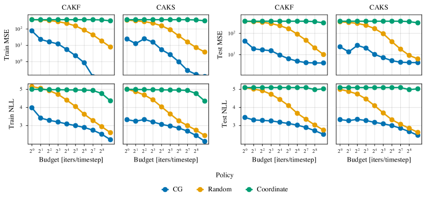
Figure C.1: Comparison of different policies for the CAKF and CAKS on the ERA5 climate dataset. The work-precision diagrams measuring MSE and NLL on the train and test set universally show that CG actions achieve lower error as a function of the budget when compared to either coordinate or random actions.

[sections]

References

- Hafner et al. [2019] Danijar Hafner, Timothy Lillicrap, Ian Fischer, Ruben Villegas, David Ha, Honglak Lee, and James Davidson. Learning Latent Dynamics for Planning from Pixels. In International Conference on Machine Learning (ICML), 2019. doi:10.48550/arXiv.1811.04551. URL http://arxiv.org/abs/1811.04551.
- Gu and Dao [2023] Albert Gu and Tri Dao. Mamba: Linear-Time Sequence Modeling with Selective State Spaces, 2023. URL http://arxiv.org/abs/2312.00752.
- Särkkä and Svensson [2023] Simo Särkkä and Lennart Svensson. Bayesian Filtering and Smoothing, volume 17. Cambridge University Press, 2nd edition, 2023. ISBN 978-1-108-91230-3.
- Rasmussen and Williams [2006] Carl Edward Rasmussen and Christopher K. I. Williams. Gaussian Processes for Machine Learning. The MIT Press, 2006.
- Evensen [1994] Geir Evensen. Sequential data assimilation with a nonlinear quasi-geostrophic model using Monte Carlo methods to forecast error statistics. Journal of Geophysical Research: Oceans, 99(C5):10143–10162, 1994. doi:10.1029/94JC00572.
- Bardsley et al. [2011] Johnathan M. Bardsley, Albert Parker, Antti Solonen, and Marylesa Howard. Krylov space approximate Kalman filtering. Numerical Linear Algebra with Applications, 20(2):171–184, December 2011. ISSN 1099-1506. doi:10.1002/nla.805. URL http://dx.doi.org/10.1002/nla.805.