Chaotic dynamics at the boundary of a basin of attraction via non-transversal intersections for a non-global smooth diffeomorphism
Ernest Fontich
Departament de Matemàtiques i Informàtica, Universitat de Barcelona (UB),
Gran Via de les Corts Catalanes 585, 08007 Barcelona, Catalonia, Spain
and
Centre de Recerca Matemàtica (CRM),
08193 Bellaterra, Barcelona, Catalonia, Spain
fontich@ub.edu, Antonio Garijo
Departament d’Enginyeria Informàtica i Matemàtiques,
Universitat Rovira i Virgili, 43007 Tarragona, Catalonia, Spain
antonio.garijo@urv.cat and Xavier Jarque
Departament de Matemàtiques i Informàtica, Universitat de Barcelona, Gran Via, 585, 08007 Barcelona, Catalonia and Centre de Recerca Matemàtica, Edifici C, Campus Bellaterra, 08193 Bellaterra, Catalonia
xavier.jarque@ub.edu
Abstract.
In this paper we give analytic proofs of the existence of transversal homoclinic points for a family of non-globally smooth diffeomorphisms having the origin as a fixed point which come out as a truncated map governing the local dynamics near a critical period three cycle associated to the Secant map. Using Moser’s version of Birkhoff-Smale’s Theorem, we prove that the boundary of the basin of attraction of the origin contains a Cantor-like invariant subset such that the restricted dynamics to it is conjugate to the full shift of -symbols for any integer or infinity.
The first author is supported by the
grant PID2021-125535NB-I00.
The second and third authors were supported by MICIU/AEI grant PID2020-118281GB-C32(33) Both grant are funded by MICIU/AEI/10.13039/501100011033/FEDER,UE. The second author is supported by Generalitat de Catalunya 2021SGR-633. We want to thank the Thematic Research Programme Modern holomorphic dynamics and related fields, Excellence Initiative – Research University programme at the University of Warsaw.
Finally, this work has also been funded through the María de Maeztu Program for Centers and Units of Excellence in R&D, grant CEX2020-001084-M funded by MICIU/AEI/10.13039/501100011033/FEDER,UE.
1. Introduction
The question of whether a dynamical system admits invariant subsets of the phase portrait in which the dynamics is chaotic goes back to the origins of this area of mathematics.
Studying the existence, or not, of chaotic dynamics and determine the topology and the geometry of the subsets where this happens has become a classical problem. Nevertheless, since the question arises in so many distinct scenarios there has been different approaches to this phenomena, including the use of non-equivalent mathematical definitions in order to capture the meaning of chaos in each particular case.
Measuring chaos in high, or even infinite, dimensional Hamiltonian dynamical systems or doing so for one-dimensional interval dynamics requires to particularize the meaning of the word chaos to concrete mathematical definitions.
Nonetheless, once we agree on which dynamical properties characterize chaos (density of periodic points, transitivity, dense orbits, sensibility with respect to initial conditions, all at once, …) a common accepted approach to ensure chaotic dynamics is to show that, in certain dynamically invariant region(s) of our phase portrait, the dynamics is conjugate (that is, equal up to a homeomorphism) to the one of a model for which it is somehow easy to test the properties mentioned above.
The usual toy model is the dynamical system , where
is the set of bi-infinite (or one-side) sequences of symbols and is the shift map; see [Mos01]. One can easily check that the system captures the dynamical properties proposed above. Since the conjugacy sends orbits of our dynamical systems to orbits of the shift map acting on the space of symbols, this methodology is also known as symbolic dynamics. To focus on the content of this paper and simplify the discussion, let us assume we have a discrete dynamical system in generated by the iterates of a (smooth) map.
In any event, the difficult part to apply this strategy is to show that in some regions of the phase portrait our dynamics is conjugate to the dynamical system . A major result in this direction goes back to the cornerstone ideas of S. Smale (Birkhoff-Smale’s Theorem) and J. Moser [Mos01] who provide checkable (in some cases only numerically) dynamical conditions to ensure that a given dynamical system has a subset of the phase portrait whose dynamics is conjugated to the full-shift of an arbitrary number of symbols (even infinitely many). Roughly speaking they showed that if a smooth map has a transversal homoclinic intersection between the stable and unstable invariant manifolds of a hyperbolic saddle fixed point then, there is an invariant Cantor set whose restricted dynamics is conjugate to .
Even though the results have been extremely helpful in many different contexts (and extended in many different directions) we emphasize that the hypotheses include three key ingredients: the hyperbolicity of the saddle point, the map is a global diffeomorphism and the transversality of the intersection of the invariant manifolds. The main goal of this paper is to address the presence of chaotic dynamics, for a concrete family of maps, under the lack of two of the conditions; the inverse map would not be globally smooth and in a first step we only can prove (analytically) that we have an intersection with a finite order contact.
Concretely, in this paper we consider the map
(1.1)
with being odd. Such map is a truncated expression of the third iterate of the (extended) Secant map applied to a polynomial near a critical period thee cycle
where (but ). See [BF18, GJ19, GJ22, FGJ24] for more details. For later discussions we point out here that is a global homeomorphism, but it is not a global diffeomorphism since the inverse map, , is not smooth over the line (see (2.1) for its particular expression).
One can easily check that the origin of (1.1) is a fixed point and its basin of attraction
(1.2)
is not empty. In [FGJ24] we proved the following topological description of
and further information about its boundary. We denote and .
Theorem 1.1.
Let odd. Then is an open, simply connected, unbounded set. Moreover, contains the stable manifold of the hyperbolic two-cycle lying in .
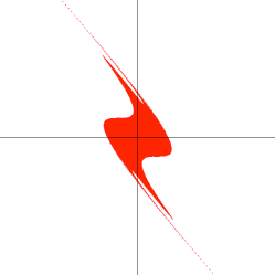
Figure 1. The picture (in red) of the set . Notice that according to Theorem 1.1 the red region is connected, simply connected and unbounded
The thesis of the above theorem glimpse the possible topological complexity of (see Figure 1). In fact, the main goal of this paper is to provide a better understanding of by proving that, apart from the stable manifold of the hyperbolic two-cycle there is a Cantor subset of where the dynamics is conjugated to the
one of the shift of symbols and so inhering all its chaotic dynamics.
In [FGJ24] we were able to describe and bound the shape of a piece of the unstable manifold of for (and it was a key point in the arguments to prove Theorem 1.1). In this paper we mimic some of the arguments there to control the shape of a piece of the stable manifold of . Using both constructions and a singular -Lemma [Ray03] we can ensure the existence of homoclinic (not necessarily linearly transversal) points for .
Theorem A.
Let be the hyperbolic two cycle lying in the boundary of . Then, the stable and unstable manifolds of (as well as ), as a fixed point for , intersect at a homoclinic point.
Going back to our previous arguments, if we want to apply Birkhoff-Smale’s Theorem we need to prove the existence of transversal homoclinic points, so that Theorem A is not enough. In [CR80] the authors are able to conclude transversal intersections under the presence of (topological) homoclinic intersections, but their map is area preserving, is a global smooth diffeomorphism and admits, in a sufficiently small neighbourhood the hyperbolic saddle, a concrete local normal form which provides a first integral.
In our case we have not the previously mentioned normal form and since is not smooth over the line we cannot use that the globalization of the stable manifold of the 2-cycle by applying is analytic. In any event, inspired in the strategy proof in [CR80], using alternative arguments to deal with our weaker conditions we are able to conclude the existence of transversal homoclinic intersections.
Theorem B.
Let be the hyperbolic two cycle lying in the boundary of . Then, the stable and unstable manifolds of (as well as , as a fixed point for , intersect transversally.
Although from the previous theorem, we have the existence of transversal homoclinic points we still cannot directly apply Birkhoff-Smale’s Theorem since the inverse map, map is not globally smooth. However, we can overcome this difficulty and prove the main result of this paper.
Theorem C.
There exists an invariant Cantor set, contained in , where the dynamics of is conjugate to the full shift of -symbols. In particular, contains infinitely many periodic points with arbitrary high period.
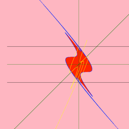
Figure 2. This picture corresponds to . In red we plot the attracting basin . In blue (respectively, yellow) we draw the stable (respectively, unstable) manifold of the two cycle . The picture illustrate (numerically) the transversal intersections described in Theorem B. According to Theorem C, contains the stable manifold of the two cycle (in blue) and a Cantor-set like with chaotic dynamics.
We emphasize that the theorems provide analytic proofs, rather than numerical evidence, of non-local properties of invariant manifolds for a family of maps. There are few cases where this has been done. For instance, in [Fon90], there is an analytical proof of the transversal intersection of the invariant manifolds for a wide range of a parameter for a class of maps which include the conservative Hénon map and the Chirikov standard map.
In [Gel99] there is an analytical proof of the transversal intersection of the invariant manifolds of the standard map when the angle is exponentially small with respect to the parameter of the family. Also, in [DRR96] and [MSS11] they prove transversal intersection for the manifolds of close to integrable maps.
We organize the paper as follows. In Section 2 we summarize some preliminaries from [FGJ24] that we need in the proofs of the present paper, trying to make the present paper self-contained. In Section 3 we prove Theorem A, in Section 4 we prove Theorem B and finally in Section 5 we conclude the proof Theorem C.
2. Preliminaries
In this section we collect some preliminary results about the map , introduced in (1.1), for , an odd number. Everything was already introduced in [FGJ24] but, for the sake of completeness and easier reading, we include them here.
The map is a polynomial and a homeomorphism and its inverse map is real analytic in , but not differentiable on the line . Its inverse is given by
(2.1)
Observe that for all . One can easily check that has a unique two-cycle , i.e., and . This two-cycle will play a fundamental role in the dynamics of . Moreover, we have that
(2.2)
A direct computation shows that the
characteristic equation of is
and the
eigenvalues and eigenvectors are given by
(2.3)
and
(2.4)
respectively.
On the one hand, it is easy to check that both eigenvalues are strictly positive. Moreover,
is strictly decreasing and is strictly increasing, with respect to the parameter . We also have
and
and
On the other hand, is negative and strictly increasing while is positive and strictly decreasing (both with respect to the parameter ). We also have
and
and
Therefore, the two cycle is hyperbolic of saddle type.
We denote , the stable and the unstable manifolds of the fixed points for the map , . Similarly we denote by , the corresponding local stable and unstable manifolds of some size that we do not make explicit in the notation. Actually, given some size ,
where denotes the open ball centered at with radius , for . We define analogously for .
We also denote
the global stable and unstable manifolds of the periodic orbit , respectively.
Since is analytic on and is analytic on the local versions of the invariant manifolds are analytic. Moreover, the (global) unstable manifold, obtained iterating by the local one, is analytic and the (global) stable manifold, obtained iterating by , is analytic except at the preimages of the intersections of with .
When there is no confusion we use the simplified notation and .
The triangle and its images: and .
In [FGJ24, Section 5] we considered the triangle of vertices
where , or equivalently,
We also considered the sets and .
We showed that the set is bounded by the images of the sides of given by the curves
, where
(2.5)
for , and
Finally, we claim that there is a (connected) piece of , tangent to the line at , contained in joining the point with some point in . We call left and right boundaries of the curves and , respectively. See Figure 3 (left). We do not include here the arguments used in [FGJ24, Lemma 5.4] to prove the claim but in the next section we mimic, including all computations, the ideas used in [FGJ24] for the case of , and .
3. Proof of Theorem A
To prove Theorem A we first show the existence of an heteroclinic intersection for the map . More precisely, we have the following statement.
Proposition 3.1.
Let be the hyperbolic two-cycle lying in the boundary of (see Theorem 1.1). Then, the unstable manifold of and the stable manifold of intersect in a heteroclinic point.
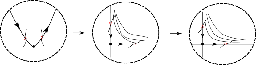
The idea is to show that (Figure 3, left) and ((Figure 3, right) intersect in a suitable manner that forces the intersection of the invariant manifolds (Figure 4).
Since the proof of this proposition is quite long, we split it into several lemmas. We assume all notation introduced in Section 2. In particular we have described the construction provided in [FGJ24, Lemma 5.4] to localize the piece of the unstable manifold attached to inside . The first step is to make
a similar construction to localize a piece of the stable manifold of . Let
(3.1)
where the inequalities follow from direct computations. We introduce the triangle with vertices
or equivalently,
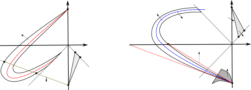
Figure 3. Left: The triangle , its image and (dashed, red) a piece of attached to . Right: The triangle , its images and , and (dashed, blue) a piece of attached to . We also add the relevant objects appearing in the proof of Proposition 3.1 and Theorem A.
As we did with the set in [FGJ24, Lemma 5.3], we study the geometry of the sets and . From the properties of these sets, we will prove that there is a piece of that is contained in . Moreover, this piece joints with a point in . See the right picture in Figure 3. Then, using the geometry of the intersection of and we will prove that and have to cross (topologically) in a heteroclinic intersection, proving Proposition 3.1. From this heteroclinic intersection we will obtain a homoclinic intersection as claimed in Theorem A.
The preimage . We denote by the image by
of the segment . Thus,
(3.2)
where
We are interested in for . Note that the point on corresponds to and is mapped by to on the line . Taking derivatives we have that
A direct computation shows that if and only if , where
and
, since, as , we have
.
It follows from these computations that has a unique minimum (in its domain) at . Finally,
which means that when meets , its tangent line is horizontal. See the right picture in Figure 3.
In other words the vectors and are parallel to the lines and , respectively.
Since is invertible (linear), for any we can represent the curve as the graph of a function (remember that ), by taking
.
Since , we have that
The convexity of implies that the image of is above its tangent line at . In case , this tangent line has slope and it is the minimum slope for all . Therefore, is above the line .
Also, has a unique minimum at . Moreover, intersects when at the point
with
Again, the convexity of the function implies that its graph intersected with is below the line
and, in particular (see Figure 3), taking we conclude that is below
(3.3)
The image . We notice that since is a two-cycle we have
so that is attached to as it was the case of .
We denote by the image by of the segment
, with . Hence, where
(3.4)
To simplify notation, we write and and unless it is strictly necessary to show the dependence in . The derivatives are given by
,,,.
Since and we have the inequalities
Then, for (odd), we have
Next lemma provides basic estimates on the parametrization .
Lemma 3.2.
Let and . The following conditions hold.
(a)
, , for , and .
(b)
with if and only if and .
(c)
for .
Proof.
The proof of the items follows from some computations based on the expressions of , and their derivatives above.
Easily . On the one hand, we have
On the other hand, where the equality only holds for and (see (3.1)). Hence (unless and where ) and so is decreasing (and negative unless ). Finally, we have . All together implies (a) and (b).
Since , the function is invertible.
If is the inverse map of , then (the image of) can be represented as the graph of the function . From its definition the function is smooth.
Lemma 3.3.
We have that is concave.
Proof.
Taking derivatives we have
From the expressions of and and their derivatives (see (3.4) and the derivatives below) we have and . Therefore
concluding and hence is concave (remember that the result is valid for all values of in the range). ∎
Now we fix . We claim that (the image of) belongs to and it is above . To check the claim, accordingly to the previous study of it is sufficient to check that is above the line introduced in (3.3). Moreover, since (the image of)
is the graph of a concave function it is enough to check that
Moreover, we also claim that is below . This easily follows from the fact that, by the description of the
preimage , the left boundary of is the graph of a convex function while
is the graph of a concave function and both graphs are tangent at .
It follows from lemmas above that we have a deep control on the left and right boundaries of , and their relative position with respect to the set . See the right picture of Figure 3. Now we close the argument by controlling the image of .
Lemma 3.4.
The upper piece of the boundary of is the
image by of the piece of the boundary
of . It can be represented as the graph of an increasing function and is contained in .
Proof.
We introduce
Taking first and second derivatives we have
First we check that, in the corresponding domain, and . This follows from
and
and
The condition implies that is invertible. Let be its inverse function
and
. The curve is the graph of and
Moreover, since
we have and .
∎
Up to this point we have completed the study of the geometry and relative positions of and (see the right picture of Figure 3). Next two lemmas show that there is a piece of attached to , being tangent to at , included in and connecting with a point in .
Let . Then we write . The first lemma characterize the dynamics of points in whose all iterates under remain in .
Moreover, the right boundary of is given by
and, by Lemma
3.2(a), .
Now, let as in the statement with . Using that
is below the line
we have that
(3.6)
First, we compute
We observe that belongs to the line .
By the definition of , we have that is less than the first coordinate
of the intersection
, i.e.,
.
Moreover, using (3.6),
Next we bound
Now we deal with the next iterate .
Since ,
and we conclude that
Consequently,
Recursively, we obtain that and this implies , Since, by hypothesis, for all we conclude that .
∎
Lemma 3.6.
The set contains a piece of joining the point with a point in .
Proof.
We will use the same argument we have used in [FGJ24].
Take any segment joining the right and left boundaries of
. By the previous lemmas, is a curve contained in joining its right and left boundaries which are outside , thus it has to cross the right and left boundaries of .
We define and, in general,
Then, is a sequence of nested compact sets and
. This set has the property that all points in are such that all their iterates stay in
and, by Lemma 3.5, converge to . Therefore, .
∎
We will see that the above description of the relative positions of and
(neighbourhoods of pieces of and , respectively) implies a heteroclinic intersection between the stable manifold of and the unstable manifold of . Unless it is necessary, we drop the dependence on the parameter .
On the one hand, in [FGJ24, Lemma 5.4] it is proven that there is a connected piece of contained in joining with some point in . On the other hand, the above lemmas show that there is a piece of contained in which joints with a point in .
We claim that the line given by , tangent to the left boundary of
at , intersects in two points the right boundary of
which is given by the curve
in
(2.5) with . If we write we have
See Figure 4. To check the claim, recall that .
We consider the auxiliary function
which measures whether is below, above or on the line .
We have
Accordingly, in order to see that has two zeros in its domain it is enough to show that there is a point in
such that . We take and, using that
, we have
Therefore, has to cross .
Next we claim that
is a segment with . To see this claim we look for the intersection of the right and left boundaries of , given by
and , respectively, with . We recall that and
The value such that is
,
and
In the same way, denoting the value such that
, we obtain
Putting together the information of the two previous claims we get that when ,
is to the right of
and that there exists some for which is to the left of and therefore
has to be at the left of
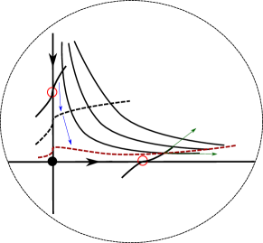
. This finish the proof of the proposition. See Figure 4.
∎
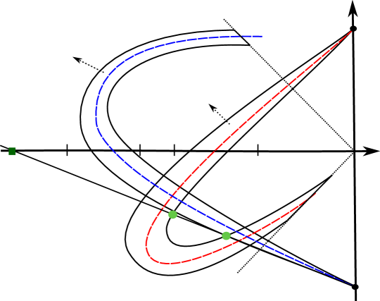
Figure 4. Sketch of the arguments providing the (topological, not necessarily transversal as it is shown in the picture) intersection of the stable and unstable manifold of the hyperbolic two-cycle (Theorem A). The green dots indicates the two intersections between and the line .
Proof of Theorem A.
Since is odd, the map is symmetric with respect to . Proposition 3.1 provides a
(maybe non-transversal) heteroclinic point in . In any case at this point the manifolds cross each other. Therefore is also a heteroclinic point. By symmetry, at the point the unstable manifold of intersects the stable manifold of . We know that the unstable manifold is analytic. The stable manifold is analytic in a neighbourhood of since the globalization of the local manifold has not meet yet. Since the manifolds do not coincide, they have a finite order contact.
Since we do not know if the intersection is transversal, we cannot apply the -Lemma of Palis in [Pal69]. However, we can apply the singular -Lemma in [Ray03].
In the two dimensional case it asserts that the iteration of a disc in the unstable manifold
accumulates in a manner to the unstable manifold of , except for an arbitrarily small neighbourhood of .
Now consider a piece of the connected component of the unstable manifold of in joining two points of the upper and lower boundaries of , respectively.
Then, by the singular -Lemma, the unstable manifold of will have discs arbitrary
-close to the unstable manifold of and therefore the discs will be in .
Finally, using the same argument as in the end of the proof of the first part of Theorem A these discs should have an intersection with the stable manifold of thus providing the desired homoclinic point.
∎
4. Proof of Theorem B
In the previous section we have proven the existence of homoclinic points associated to the stable and unstable of the cycle . Using this fact, in this section we demonstrate that stable and the unstable manifolds of intersect in a transverse homoclinic point. Our approach is inspired in the work of [CR80]. However, there is an important difference. In [CR80] the authors deal with analytic area preserving maps and can use tools as the Birkhoff normal form, while our map is not area preserving and it is not an analytic diffeomorphism. Our presentation uses the special structure of the map and the fact that we can linearize the map around which a conjugation.
For the point we will denote by
the local stable, local unstable, global stable and global unstable manifolds associated to for the map , respectively. The size of the local manifolds will be as small as we need.
We split the proof of Theorem B into several lemmas. Given we let be the open ball centered at and radius .
Lemma 4.1.
Let be small enough. Then, there exist two points and in such that
Moreover, there exist analytic local parametrizations of around
and of around
given by with
and with
for some small.
Since the manifolds do not coincide, the above intersections (at the points and ) have finite order contact.
Fix small enough such that
and . We denote by the piece of and by the piece of .
Proof.
Fix small enough and consider local manifolds contained in . Let be the point determined by the topological transversal intersection of the stable and the unstable manifolds of for the map given by Theorem A. By iterating forward this point by and we obtain the existence of and in , respectively. Moreover, since and are analytic we have that intersect with finite order contact (otherwise they would coincide). Then, there exists as claimed. By construction, there exists such that
According to the previous arguments if
(4.1)
then intersect at , is analytic in a neighbourhood of and the intersection has a finite order contact and the lemma follows. Now, we consider the case that there exists a finite sequence of natural numbers , , such that
(4.2)
Note that , and hence, . First, we deal with , the first time the globalization of meets so that is analytic from to this point. Thus, near the stable manifold ,
is analytic and can be parametrized as
where , , are analytic, satisfy and and is small enough. Since we have
where .
Since is odd we can reparametrize the curve using the new parameter to obtain analytic and
with , .
We conclude thus that admits an analytic parametrization in a sufficiently small neighbourhood of . Repeating the same procedure a finite number of times it is clear that intersects with finite order contact at the point .
∎
The translation
moves to the origin. For simplicity we write the new coordinates again as . Observe that (in the new coordinates) and that
(4.3)
The eigenvalues and eigenvectors are given in
(2.3) and (2.4), respectively.
We will denote
(4.4)
(we drop the dependence on unless it is strictly necessary). We recall from Section 2 that
(4.5)
We parametrize the local stable and unstable manifolds associated to the origin by the -variable so that the expressions can be written as and , respectively. We obviously have
(4.6)
Next step is to introduce local analytic coordinates
around so that the expression of the local stable and unstable manifolds would be and , respectively.
Lemma 4.2.
We consider the local change of variables
Then, for small enough the local expression of in is given by
where
Moreover, the local change of coordinates, , is analytic.
Proof.
We claim that the new variables define a local change of coordinates around the origin. Indeed, since and are analytic, by the Inverse Function Theorem we only need to check that
is non-singular and this is a direct consequence of (4.5).
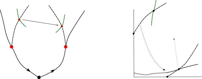
Clearly is a local analytic diffeomorphism. See Figure 5.
∎
Figure 5. The changes of coordinates corresponding to Lemma 4.2 and Lemma 4.4. In fact in this figure includes a primer change of coordinates to move to the origin.
We will see next that is -conjugate to its linear part . For this we will apply Sternberg’s Theorem [Ste58, Theorem 1]. The following lemma checks a key hypothesis of that theorem.
Lemma 4.3.
The eigenvalues and of the linear part of at given in (4.4) and (2.3) are non-resonant.
Proof.
We first note that (the determinant of ). It is easy to check by induction that
and
where , and is not a perfect square.
This means that for all .
In case (a), since and the previous equality is impossible.
In case (b), cannot be 0. Then, so that (4.9) is also impossible.
Concerning resonances of the form (4.8) the argument is completely analogous.
∎
Theorem 1 in [Ste58] provides a local change of coordinates conjugating to its linear part .
From it we will obtain a near the identity conjugation.
Lemma 4.4.
There is a conjugacy from to its linear part at the origin of the form
(4.10)
where , are functions defined in a sufficiently small neighbourhood of the origin with .
Proof.
Let be the local conjugacy given by Sternberg’s Theorem. Consequently, should send the stable and unstable manifolds of to the corresponding ones of , which in this case means that it preserves the axes.
Writing , this is translated into the conditions and . Then,
with ,
and analogously
with .
Since is a diffeomorphim, .
We write .
We claim that is also a conjugation from to . Indeed, since commutes with ,
Moreover, is of the form given in (4.10). See Figure 5.
∎
In Lemma 4.1 we have proven the existence of the points
Then, we can use the changes of coordinates introduced in the previous lemmas to transport those curves to a neighbourhood of the origin. Denote by and the parametrizations of and , respectively. We focus on the pieces of and in the first quadrant. Without loss of generality we can assume that these pieces are parametrized by .
Lemma 4.5.
The curves and intersect the coordinate axes and
at points and and have a finite order contact there, respectively. Moreover, for small enough we have that , admit the following parametrization
(4.11)
where for , , , and are functions with , for .
See Figure 6.
Proof.
The lemma follows from the fact that and are points of finite order contact between the stable and the unstable manifolds of and the change of coordinates we have used is .
∎
Figure 6. Sketch of the situation described in Lemma 4.5.
We want to show that, for large enough, and intersect transversally. This framework is quite close to the one in [CR80, Theorem 1.1] but in their case the linear map admits the function as a first integral, which is not our case. Then, we provide a proof in our case to get the same conclusion.
Given and introduced in (4.4)
and (2.3) and we
consider the auxiliary interpolation map
We also consider the first quadrant and defined by
(4.12)
It is continuous and real analytic in the interior of .
Lemma 4.6.
The function is a first integral of , , in .
Proof.
To prove the lemma we compute
∎
Next step is to show that there exist reparametrizations , ,
of the curves , which have a useful property.
Lemma 4.7.
There exist continuous reparametrizations , , of the curves given by , , that are in and they satisfy
for some small enough.
Proof.
For we impose the condition to obtain . Using (4.11) and (4.12) we have
(4.13)
We have , .
Consequently, by the Inverse Function Theorem, is locally invertible
and we can write
(4.14)
for for some small.
For , arguing as above, we have
Analogous computations imply that and
(4.15)
∎
The following lemma establishes a relation between and .
Lemma 4.8.
Let be small enough. Then, there exists a function , such that
Moreover
(4.16)
In particular, there exist in and a sequence of positive values , such that and for every .
Proof.
Let be as in Lemma 4.7. We use the following notation
We define
and therefore
(4.17)
Clearly, is in .
Next, we will check that . Using that is a first integral and Lemma 4.7 we have that
since
and
.
Using
and the fact that is a function in its domain we get from Bolzano’s Theorem that there exist such that for every there exists such that , and the lemma follows.
∎
The lemma above shows that the curves and intersect at the values . Next lemma shows that these intersections, for large enough, are transversal.
Lemma 4.9.
Let be large enough. The following limits hold.
(4.20)
In particular, for large enough, the curves and intersect transversally at the values .
Proof.
To prove the lemma we first make some computations. From the proof of Lemma 4.7, and equations (4.14) and (4.15), we deduce the following asymptotic behaviours (as )
(4.21)
where
are non-zero. Hence, using (4.11), we can compute the following expressions for some of the terms of the numerator and denominator in (4.20).
On the one hand, we have
On the other hand, we have
From (4.17) and (4.18) evaluated at the values of corresponding to we can also conclude that
and
All together allows us to compute the limits of the statement
∎
End of the proof of Theorem B.
Let satisfy the conditions of the previous lemmas. We consider the sequence of points
(4.22)
From Lemma 4.9,
and intersect transversally. It follows from (4.11) and the lemmas above than
To conclude the proof of Theorem B we argue as follows. We know that and . Also the stable and unstable manifolds are invariant sets for the map . Finally, Lemma 4.9, definition (4.24) and equation (4.25) imply that and correspond to transversal intersections of the stable and unstable manifolds of accumulating to the points and , respectively. See Figure 7.
∎
Figure 7. Sketch of the proof of Theorem B with the points and being transversal intersections of the stable and unstable manifolds of (for ).
5. Proof of Theorem C
The proof of Theorem C is based on Moser’s version of Birkhoff-Smale Theorem, concretely we will apply Theorem 3.7 in [Mos01] in our setup. The key difficulty
comes from the fact that, in our case, is not differentiable on the line . Therefore, we need to make sure that the construction in [Mos01] can be made so that we only have to deal with our map and its inverse in a domain that does not meet the line . However, notice that both the stable and the unstable manifolds of the two-cycle cross the line . See Figure 2.
Remark 5.1.
It follows from Lemma 4.1 that as well as intersect the line at isolated points. In other words, finite length pieces of and only contain finitely many intersections with .
Let be a neighbourhood of as in Lemma 4.4 where we can take local coordinates
for which is located at and
the stable and the unstable manifolds of are the vertical and horizontal axes, respectively. Assume also that .
In the following items, we summarize notation and facts of the constructions we have made in the previous section that will be important in the proof of Theorem C. See Figure 8.
(a)
Let be the homoclinic point given in Theorem A and and , , be the points given in Lemma 4.1.
Let and introduced after the statement of Lemma 4.1. Then
and . Moreover, taking we have that
(b)
Let and be the points introduced in
(4.24). We have that
and are transversal homoclinic points,
and
(c)
Let
and
.
(d)
We consider the points
As a consequence of the previous items we have
(e)
For any and , if we write,
we have that
(5.1)
In particular, considering and as large as necessary we know that the corresponding points and are as close as needed to the point , and, by the -Lemma [Pal69] they are transverse homoclinic points with tangent vectors close to the tangent vectors of the local manifolds.
Proof of Theorem C.
Let be a neighbourhood of .
Assume it is sufficiently small so that
is contained in . Clearly, is a neighbourhood of . From items (b) and (d) there exists such that and for all .
Let be large enough and let be a small neighbourhood of (suitable size will be decided later on). Then is a neighbourhood of and, if we denote
then is a neighbourhood of .
Let be a pseudo-rectangle in the first quadrant attached to whose boundaries are given by pieces of and and the others are just straight lines (parallel to the tangent lines of and at ).
Define
(5.2)
If we iterate by , while staying in where the dynamics is conjugate to the one of the linearization at , we eventually meet .
Following Moser we introduce the transversal map . Given we consider a number of iterates bigger that of . By construction . Next we consider to be the smallest integer such that and , , if it exists. We denote by the set of such that exists and we define
by
(5.3)
To apply Moser’s Theorem we should check that the restriction of to is a diffeomorphism or equivalently that .
That is, we should prove that, by choosing small enough the points travelling from to itself would not meet the line , where is not smooth.
Since and is a small neighbourhood of the iterates of will travel
following the orbit of
until they arrive to . Then, by item (b), from to the iterates will stay in .
Hence, the only iterates of points which might fall in the line are the iterates needed to go from to and the ones from to . To finish the argument, we distinguish two cases.
Case 1. The finite set does not intersect . By continuity there exists a sufficiently small open neighbourhood of such that the open set
does not intersect either.
Of course, by items (b) and (d) there are infinitely many points of the sequences belonging to .
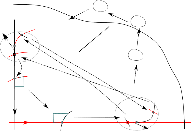
Choose (the neighbourhood of above) small enough and large enough such that and such that belong to , for . Choose and define as in (5.2). By construction, the map is well defined and , it has an inverse which is also since no iterates of or in the definition of (see (5.3)) intersect .
Figure 8. The illustration of all items (a)-(f).
Case 2.
The set intersects .
Let ,
for , for some , be the intersection.
We recall that the
stable and unstable manifolds of the point have discrete intersection with .
Again, items (b) and (d) imply that we can choose large enough such that there exist two small open neighbourhoods of and of such that for all we have that
We are in the same situation as in the previous case. Therefore, choosing (the neighbourhood of above) small enough and large enough we obtain the regularity claim for
and .
Now, Theorem 3.7 in [Mos01] implies that there is a Cantor set contained in and a homeomorphism from to the space of sequences of symbols () which conjugates with the Bernoulli shift and, as a consequence,
there is a dense set of periodic orbits of
, and therefore of and in .
Moreover, Theorem 3.8 in [Mos01] implies that there is a dense subset of homoclinic points to in . We recall from Theorem A (b) of [FGJ24] that . Finally, since
,
that is, the boundary of has infinitely many periodic orbits with arbitrary high period.
∎
References
[BF18]
Eric Bedford and Paul Frigge.
The secant method for root finding, viewed as a dynamical system.
Dolomites Res. Notes Approx., 11(Special Issue Norm
Levenberg):122–129, 2018.
[CR80]
Richard C. Churchill and David L. Rod.
Pathology in dynamical systems. III. Analytic Hamiltonians.
J. Differential Equations, 37(1):23–38, 1980.
[DRR96]
Amadeu Delshams and Rafael Ramírez-Ros.
Poincaré-Melnikov-Arnold method for analytic planar maps.
Nonlinearity, 9(1):1–26, 1996.
[FGJ24]
Ernest Fontich, Antoni Garijo, and Xavier Jarque.
On the basin of attraction of a critical three-cycle of a model for
the secant map.
Preprint, 2024.
[Fon90]
E. Fontich.
Transversal homoclinic points of a class of conservative
diffeomorphisms.
J. Differential Equations, 87(1):1–27, 1990.
[Gel99]
V. G. Gelfreich.
A proof of the exponentially small transversality of the separatrices
for the standard map.
Comm. Math. Phys., 201(1):155–216, 1999.
[GJ19]
Antonio Garijo and Xavier Jarque.
Global dynamics of the real secant method.
Nonlinearity, 32(11):4557–4578, 2019.
[GJ22]
Antonio Garijo and Xavier Jarque.
Dynamics of the secant map near infinity.
J. Difference Equ. Appl., 28(10):1334–1347, 2022.
[Mos01]
Jürgen Moser.
Stable and random motions in dynamical systems.
Princeton Landmarks in Mathematics. Princeton University Press,
Princeton, NJ, 2001.
With special emphasis on celestial mechanics, Reprint of the 1973
original, With a foreword by Philip J. Holmes.
[MSS11]
Pau Martín, David Sauzin, and Tere M. Seara.
Exponentially small splitting of separatrices in the perturbed
McMillan map.
Discrete Contin. Dyn. Syst., 31(2):301–372, 2011.
[Pal69]
J. Palis.
On Morse-Smale dynamical systems.
Topology, 8(4):385–404, 1969.
[Ray03]
Victoria Rayskin.
Multidimensional singular -lemma.
Electron. J. Differential Equations, pages No. 38, 9, 2003.
[Ste58]
Shlomo Sternberg.
On the structure of local homeomorphisms of euclidean -space.
II.
Amer. J. Math., 80:623–631, 1958.