Quantum computing with Qiskit

Abstract

We describe Qiskit, a software development kit for quantum information science. We discuss the key design decisions that have shaped its development, and examine the software architecture and its core components. We demonstrate an end-to-end workflow for solving a problem in condensed matter physics on a quantum computer that serves to highlight some of Qiskit’s capabilities, for example the representation and optimization of circuits at various abstraction levels, its scalability and retargetability to new gates, and the use of quantum-classical computations via dynamic circuits. Lastly, we discuss some of the ecosystem of tools and plugins that extend Qiskit for various tasks, and the future ahead.

I Introduction

Quantum computing is progressing at a rapid pace, and robust software tools such as Qiskit are becoming increasingly important as a means of facilitating research, education, and to run computationally interesting problems on quantum computers. For example, Qiskit was used in a recent paper that showed evidence of utility for quantum computers by using error mitigation kim2023evidence. It was also used in a demonstration of fault-tolerant magic state preparation beyond break-even fidelity gupta2023encoding, and the preparation of ground states for Heisengberg and Schwinger models on 100⁺ qubit systems farrell2023scalable; yu2023simulating.

Qiskit was started in 2017 as an open-source toolbox for quantum computing by IBM. Six years after its initial release, the Qiskit ecosystem is thriving. The package has been installed over 6 million times, at a current rate of 300,000 per month. 500⁺ individuals have contributed to its development, the vast majority of whom are unaffiliated with IBM. 300 packages in the Python Package Index (PyPI) depend on Qiskit, as well as hundreds of other code repositories on Github github; pypi. More than 2,000 scientific papers posted to arXiv have used Qiskit, and many university courses have used Qiskit in their material. By a large margin, Qiskit is the most widely-adopted quantum computing software unitaryfund.

Recently Qiskit reached a 1.0 major release milestone. In this paper we overview the software’s design philosophy and overall architecture. We also showcase some of its capabilities through end-to-end examples, and discuss the software ecosystem that has formed around it.

The rest of this paper is organized as follows: Section II discusses the main design decisions and the driving philosophy behind Qiskit. Section III gives an overview of the software architecture, with a deeper dive into circuits, operators, pass managers and primitives, which form the core components of Qiskit. We combine these in Section IV to show an example workflow where a Hamiltonian simulation problem is solved using Qiskit on a quantum computer. We demonstrate how Qiskit can be leveraged to improve the experimental performance using a variety of techniques, including by targeting hardware-native gatesets and leveraging dynamic circuits. Section LABEL:sec:ecosystem illustrates some software tools from the community that have built on Qiskit, and Section LABEL:sec:conclusion concludes the paper with a look towards the future.

II Design Philosophy

We begin by discussing Qiskit’s scope within the broader quantum computing software stack, as illustrated in Figure 1. Starting from a computational problem, a quantum algorithm specifies how the problem may be solved with quantum circuits. This step involves translating the classical problem to the quantum domain, for example Fermion to qubit mapping qiskit-nature; mcclean2020openfermion. Circuits at this level can be quite abstract, for example only specifying a set of Pauli rotations, some unitaries, or other high-level mathematical operators. Importantly, these abstract circuits are representable in Qiskit, which contains synthesis methods to generate concrete circuits from them. Such concrete circuits are formed using a standard library of gates, and may now be represented using intermediate quantum languages such as OpenQASM and QIR cross2022openqasm; mccaskey2021mlir.

The transpiler rewrites circuits in multiple rounds of passes, in order to optimize and translate it to the target instruction set architecture (ISA). The word “transpiler” is used within Qiskit to emphasize its nature as a circuit-to-circuit rewriting tool, distinct from a full compilation down to controller binaries which is necessary for executing circuits. But the transpiler can also be thought of as an optimizing compiler for quantum programs.

The ISA is the key abstraction layer separating the hardware from the software, and depends heavily on the quantum computer architecture beneath. For example for a physical quantum computer based on superconducting qubits, this can include $\tt CNOT$, $\tt\sqrt{X}$ and $\tt RZ(\theta)$ rotations. For a logical quantum computer, it can include joint Pauli measurements, magic state distillation, or other operations specific to the error correcting code beverland2022assessing. Note that the ISA is often more than just a universal set of quantum gates, and can include classical control-flow such as if branches and while loops, or limited concurrent classical computations on classical data.

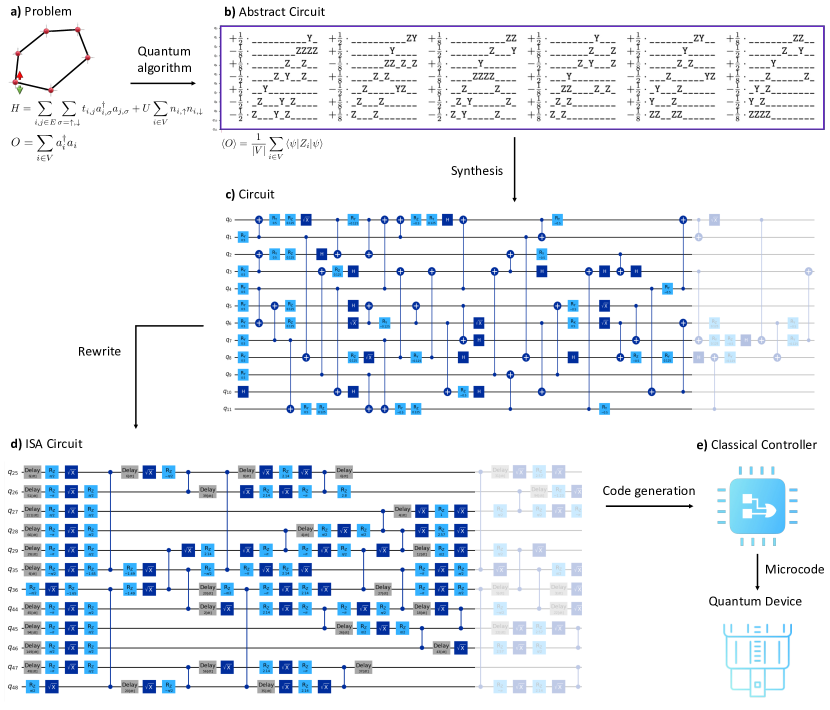
Figure 1: The quantum computing software stack at various abstraction levels. Qiskit’s scope spans the middle-end from (b) to (d), which includes all the tools and algorithms needed to efficiently represent and compile circuits. a) A representation of the problem and the observable to be measured, for example the dynamics of a Fermi-Hubbard model. b) Translation of the problem to an abstract Hamiltonian simulation circuit, represented by exponentials of Pauli operators. c) Synthesis of the high-level operators to standard gates, yielding a circuit with gates from a standard library. d) ISA circuit that is compatible with the hardware’s instruction set, where all gates and their schedule is explicit. The ISA is a feature of the underlying quantum computer, and differs among various technological platforms and between fault-tolerant vs. pre-fault-tolerant quantum computers. e) Classical code generation for a controller to execute the ISA circuit on the quantum device.

In the rest of this section we discuss some key design decisions that have informed Qiskit’s development.

II.0.1 Modularity and extensibility

Quantum computing is an active area of research huang2020predicting, and major advances in many areas are needed to solve interesting and classically intractable problems. Qiskit is built as a tool to explore quantum computing and drive innovation. As such, modularity and extensibility are principal driving forces behind the software design. For example, it is straightforward extend its library of circuits or circuit synthesis and optimization methods. These can be completely outside of Qiskit, visible to Qiskit only via a plug-in interface, so that research code can be seamlessly used by Qiskit users. In Section LABEL:sec:ecosystem we give examples of some projects that extend Qiskit in interesting ways using this mechanism.

II.0.2 Balance between performance and rapid prototyping

Speed is a fundamental consideration for large-scale quantum computing, and software performance must not hinder the overall workflow. As quantum computers scale, larger and larger circuit volumes must be analyzed and transformed rapidly. In addition, many quantum algorithms as well as error mitigation protocols require a large number of circuit executions peruzzo2014variational; van2023probabilistic. As such, Qiskit places a significant focus on speed. Performance-critical components and algorithms are written in the Rust programming language 10.1145/2663171.2663188, and performance is tracked over time using extensive benchmarks asv. However, Python remains the language of choice for many in the scientific community due to its ease of adoption and lower barrier of entry. By moving only the performance-critical aspects of the code to Rust (currently about 6% of the code base), Qiskit maintains a Python environment for programming and prototyping, striking a balance between speed and ease of use.

II.0.3 Balance between portability and hardware optimization

Qiskit uses universal circuit representations and transformations that are agnostic to the underlying hardware. This enables writing quantum programs in a natural manner, without having to worry about implementation details. However, Qiskit is also able to transform circuits to make them compatible with diverse quantum platforms with different instruction set architectures, such as superconducting or trapped-ion technologies qiskit-ibm-runtime; qiskit-ionq; qiskit-rigetti. Qiskit can represent many types of quantum hardware through its Target class, which is an abstract machine model. The Target defines a model for describing the instructions available on quantum hardware, their properties such as error rates, and other constraints of the hardware. Qiskit’s transpiler is retargetable, and can use this information to optimize the circuit for a given hardware.

II.0.4 Levels of abstraction and full-stack integration

Another goal in Qiskit’s evolution has been to give more control to users by allowing them to program at different abstraction levels. A high level programming model is attractive since it allows users to focus on code development and not worry about the details that go into realizing a given computation on a physical machine. Other users may want to investigate the physics behind quantum computing, through timing and dynamics of gates. All of these abstraction level are compatible with each other in the same Qiskit circuit, and optimizations that cut across these layers are often employed to save on resources, for example direct synthesis of high-level operators for a given Target, without intermediary steps that may prolong circuit depth.

II.0.5 Quantum-classical integration: real time and near time

Quantum computation is often more than just a unitary time evolution of quantum states. Classical resources must be tightly integrated with quantum computers to enable different kinds of computation, such as using classical control flow to extend the computational reach of quantum circuits bravyi2020quantum or to correct errors bravyi2005universal, or using classical computation to optimize the parameters of a quantum circuit peruzzo2014variational

We distinguish between two types of classical computation. The first are “real-time” classical computations that occur while qubits are coherent, such as control flow based on the outcome of qubit measurements. We call circuits of this type dynamic circuits, as the instructions that are executed are determined dynamically as the circuit progresses. Qiskit’s circuit model allows for a rich mixture of classical operations concurrent with quantum operations, similar to the circuit model defined in the OpenQASM 3 cross2022openqasm language.

The second type of classical computation occurs in a “near-time” environment, which does not have the same stringent timing requirements, but must still occur with low latency. Examples include parameter binding, just-in-time compilation, optimization of circuit parameters, or learning noise models. Qiskit is designed to be a lightweight framework that can be integrated into a runtime environment that co-locates quantum with general-purpose classical processors, so that thousands of circuits can be rapidly generated and evaluated in a dynamic manner to provide the final solution. An example of this runtime environment is the Qiskit Runtime implemented in IBM systems.

II.0.6 Computational primitives

Beside specifying the quantum circuit, the computation’s output is also a key consideration. In quantum computing there exist two main primitives for capturing the output of a quantum circuit: sampling output bitstrings, or estimating observable expectation values. These primitives are the means by which circuits are evaluated in Qiskit. They define a common interface, even if the implementation details can vary significantly. For example, efficient estimators are an active area of research huang2020predicting; elben2023randomized, as are error mitigation methods that can improve their results van2023probabilistic; kim2023evidence. Nonetheless, they all follow a simple interface of taking a (possibly parameterized) circuit, coupled with one or more observables, and returning estimates of their expectation values. Different estimators can thus be exposed to Qiskit as a primitive.

II.0.7 Four-step workflow

A common pattern for using Qiskit is through a four-step workflow, and the software architecture reflects this (see Figure 2). First, a classical problem is mapped to quantum computation by generating circuits that encode the problem. This step is best handled by domain-specific software or experts, although Qiskit provides a convenient circuit construction API that can handle large circuits. Next, the circuits are transformed to make them amenable for execution on a target hardware. We generically refer to this step as transpilation, as it is a circuit-to-circuit rewriting step, and not a full compilation down to the classical controller instructions. Next, the circuits are evaluated using primitive computations on a target backend. Finally, the results are post-processed to obtain a solution to the original problem. Qiskit provides interfaces so advanced workflows following these basic steps can be enhanced with new techniques. For example, a common pattern is to iteratively generate new circuits that depend on the results obtained from a previous batch of circuits, which can be seen as a loop around the last three steps above cerezo2021variational.

II.0.8 Integrated visualizations

A popular feature of Qiskit are its visualization capabilities. This includes advanced circuit visualizers that display large circuits of varying characteristics (e.g. see Figure 3), target visualizer for giving an overview of the hardware topology and supported gates, and state and distribution visualizers for understanding computational outputs. Other types of information useful for debugging, such as the sequence of passes in the transpiler or the graph structure of the circuit can also be visualized.

II.0.9 Tensor ordering convention

When interpreting circuits, a convention must be picked for the ordering of qubits in a register, arguments of all instructions, and of instructions themselves. For example it is common that instructions in a circuit are ordered from left to right (i.e. temporal ordering), which is the opposite of how gate matrices are multiplied in the circuit.

Throughout Qiskit, tensor products are ordered as $Q_{2}\otimes Q_{1}\otimes Q_{0}$. For example the Pauli $ZX$ means $Z_{1}X_{0}$. In this convention, the computational basis can be conveniently represented as $\ket{000}=\ket{0}$, $\ket{001}=\ket{1}$, $\ket{010}=\ket{2}$, $\ket{011}=\ket{3}$, etc. This leads to more natural representations of reversible circuits too, as numbers are encoded in qubit registers in the same way as they would be in classical registers. Note that this is merely a convention, which may be natural for some tasks but not others. For example, the qubit arguments to a $CX$ instruction are ordered as $Q_{0}=\text{control}$ and $Q_{1}=\text{target}$, This leads to a unitary of $CX=\begin{bmatrix}1&0&0&0\\ 0&0&0&1\\ 0&0&1&0\\ 0&1&0&0\end{bmatrix}$, which may be different to some textbook definitions of the gate nielsen2001quantum. The unitary can be changed, however, by simply using it in the circuit context as $CX(Q_{1},Q_{0})$. Similar qubit ordering conventions have been adopted elsewhere in the literature smith2017someone; quirk.

III Software Architecture

In this section we give an overview of Qiskit’s architecture, which is shown in Figure 2. We then expose more details on circuits, pass managers and primitives, which form the backbone of the software.

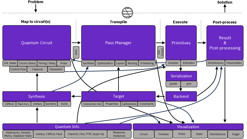
Figure 2: Qiskit’s software architecture.

The core component in Qiskit is the quantum circuit, around which the rest of the framework revolves. The quantum info module serves as a toolbox to connect circuits to the mathematical formalism of quantum information. Beside tools for representing channels and measuring fidelities, it includes operators that can be used in building abstract circuits, or be used for observable measurements. The transpiler transforms quantum circuits by applying a pipeline of passes on them, orchestrated by a pass manager. Circuit transformations occur according to a target, which is an abstract machine model that summarizes the pertinent features of a backend for the pass manager, such as its instruction set architecture (ISA) and any properties or constraints associated with it. Primitives evaluate circuits via backends, which may consist of simulators or hardware. Qiskit supports two types of circuit serialization, one based on the OpenQASM language cross2022openqasm and one based on a backwards-compatible Qiskit-native binary representation called QPY. Finally, circuits are evaluated with respect to some primitives, such as observable expectation values or measurement samples. These can be post-processed to obtain a solution, or be used to generate a next set of circuits.

III.1 Circuits

Quantum circuits form the core component of Qiskit. Circuits express a particular computation as a time-ordered set of instructions, which can then be transformed and analyzed by the rest of the software.

Circuits in Qiskit are defined very broadly — any operation on quantum or classical data can be included in the circuit. This includes standard operations such as qubit resets, gates and measurements, but also higher-level mathematical operators such as unitaries, isometries, Cliffords or Fourier transforms. Circuits may contain real-time classical computation on classical data while qubits are coherent, such as Boolean functions applied to the outcome of measurements, as well as real-time classical control flow like loops and branching. Qiskit circuits may also describe the timing of operations and even continuous-time dynamics of qubits via pulse-defined gates. Any of these levels of abstraction may be mixed and matched within the same circuit, and circuits can be composed with each other like building blocks. We use these different types of circuits in Section IV to solve the same problem in a variety of ways.

Figure 3 shows some examples of the various types of circuits that can be described in Qiskit. This flexibility enables the study of a wide variety of quantum algorithms and physical implementations. Owing to the flexibility of the circuit data structure, it is easy to extend it beyond its default scope, and we illustrate some examples of this in Section LABEL:sec:ecosystem.

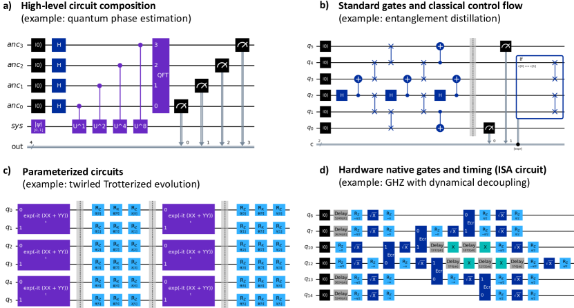
Figure 3: Examples of different kinds of circuits in Qiskit. All circuits are visualized using Qiskit. a) A quantum phase estimation algorithm kitaev1995quantum. The circuit is built using standard gates as well as some high-level blocks: state preparation $\ket{\psi}$, unitaries raised to a power and controlled, and quantum Fourier transform. The transpiler decides how to synthesize the circuit efficiently from this high-level representation. b)An entanglement distillation circuit that performs a pipelined preparation of three Bell states using gates from the standard library. Two of the pairs are distilled into one bennett1996mixed, and in the event that the distillation fails, the protocol falls back on the third pair, thereby avoiding post-selection failure. This latter operation is described by a classical if statement on measured qubit outcomes. c) A Trotterized $XX+YY$ Hamiltonian simulation lloyd1996universal circuit, with each layer’s coherent noise suppressed by Pauli twirling bennett1996purification. This light-weight circuit pattern can turn into many circuit instances on the fly by substituting different time evolution parameters or angle parameters to sample different twirls. d) A GHZ state preparation circuit. This circuit is lowered to the native instruction set architecture (ISA) of a hardware where instruction durations are known from calibrations. The precise timing allows control techniques such as dynamical decoupling viola1999dynamical to be applied that refocus the noise in hardware.

Distinct from how users interact with circuits in Qiskit, the internal representation of circuits can take multiple forms, each suitable for specific purposes. The default data structure is a list of instructions (i.e. operations applied to quantum or classical data). However, in many circuit rewriting algorithms a data-flow graph structure, represented by a directed acyclic graph (DAG) is more suitable, since it makes the succession of operations and flow of information explicit. Likewise, some circuit rewriting algorithms benefit from a canonical graph form where gate commutations are taken into account and only true dependencies between instructions are encoded. Particularly structured sub-circuits may also be temporarily converted to specialized data structures to facilitate reasoning about the circuit at a more abstract level, for example Boolean linear functions patel2008optimal, Cliffords aaronson2004improved, or phase polynomials amy2014polynomial .

Given the quantum circuit’s central role, a particular emphasis in these data structures is to make circuits as light weight as possible. For example, certain common gates are defined as singletons in the standard library, blocks can be reused in circuits, and circuit synthesis and lowering for abstract operations is lazily deferred to the transpiler. This ensures that the software remains scalable as increasingly larger quantum computations are studied.

III.2 Pass Manager

The Qiskit transpiler contains a collection of passes implementing proven translation and optimization techniques on top of a flexible framework for describing, composing and running pipelines of quantum circuit transformations. This enables authors of both high-level abstract quantum circuits and low-level hardware-aware quantum circuits to benefit from both Qiskit’s included passes to generate a device-compatible and device-optimized implementation of their input circuit as well as an API for automating circuit transformations.

As Qiskit circuits support multiple levels of abstraction, although the circuit is progressively lowered and transformed, the output representation of the transpiler is also a quantum circuit. This architecture promotes inspection, characterization and modification of transpiled circuits using the same tooling available for circuit construction, aiding users in understanding their circuit’s execution cost relative to a finite error budget, and facilitates experimentation with alternative optimization techniques which may bring advantages for specific applications or device architectures to take maximal advantage of modern device capabilities.

Underlying the transpiler is a pass-based infrastructure called the Pass Manager which supports the construction and manages the execution of composable and re-usable pipelines of semantic-preserving transformations for quantum circuits, including logic for controlling the flow of the compilation pipeline depending on device or circuit characteristics, or properties of the intermediate compilation steps. This architecture is similar to classical compiler infrastructures such as LLVM lattner2004llvm.

Qiskit defines a series of standardized stages of compilation, each comprised of one or more transformation and analysis passes, which in turn define standardized hook points for transpiler plugins and extensions to modify or extend the predefined Pass Managers defined and distributed with Qiskit. These Pass Managers encapsulate best-practices in circuit optimization, translation and re-writing for a broad set of applications and hardware architectures, and serve as the basis for full-pipeline compiler performance comparisons for experimentation and extensions.

III.3 Primitives

Finally, circuit executions are performed using primitives, which provide a consistent API for performing common quantum computational tasks. In particular, the primitives consist of a sampler and estimator. Samplers return measurement outcomes, while estimators return post-processed expectation values.

The primitives can be implemented in a Qiskit runtime environment, which provides a tightly-coupled interface of quantum-classical compute. Note that this is distinct from real-time classical compute which must occur at a much higher speed and is consequently much more limited in scope. By co-locating general-purpose classical computers with the quantum processor, a runtime environment can cut down the latency on the execution of quantum-classical workloads. This could consist of optimizing circuits to suppress errors, generating and running extra circuits for error mitigation, post-processing results or updating parameters.

IV Qiskit by Example

We now show an end-to-end example that uses Qiskit to solve a problem in condensed matter physics on a quantum computer. The purpose is to highlight general workflows for solving problems using Qiskit, and some of the software’s capabilities. Specifically, we consider the kicked Ising model for a lattice of spins. This problem is widely studied in statistical mechanics and was the subject of the large scale “quantum computer utility” experiment performed in kim2023evidence. In one instance, we show how changing the target to include new calibrated gates automatically prompts the transpiler to re-target and re-optimize the circuit to reduce depth. In another instance, we show how Qiskit’s dynamic circuit capabilities can make shorter and more reliable circuits especially when faced with limited connectivity.

IV.1 Ising model simulation on a quantum computer

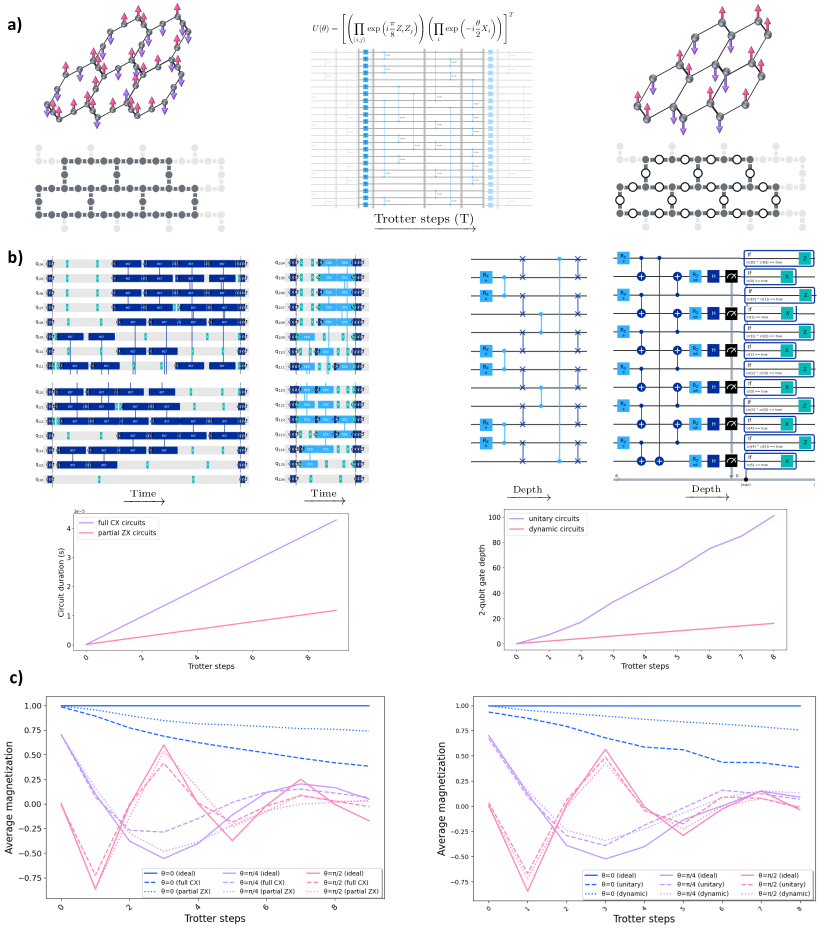
Figure 4: Using Qiskit to solve a Hamiltonian simulation problem on a quantum computer. a) Building a (parameterized) circuit to represent the problem. We consider a heavy-hexagonal as well as honeycomb lattice of spins. The former matches the lattice of hardware qubits, while the latter does not. The Hamiltonian simulation consists of multiple Trotter steps that alternate $X(\theta)$ rotations with $ZZ(\pi/8)$ interactions on the edges of the lattice. Throughout this figure, the left (right) side corresponds to the heavy-hexagonal (honeycomb) lattice. b) Four circuits post-transpilation, each realizing a single Trotter step. Left: the transpiler lowers the circuit to the hardware ISA and inserts dynamical decoupling. The availability of new, shorter gates will prompt Qiskit to retarget the circuit to shorten its duration. Right: the transpiler uses SWAP gates to map the honeycomb lattice to the hardware. When we use dynamic circuits, we gain a reduction in depth. c) Experimental results using Qiskit primitives. Here we use the Estimator to obtain expectation values corresponding to the average magnetization of the spin system. The Estimator is invoked with built-in readout error mitigation, and $\theta$ parameters are substituted at runtime. Left: we see an improvement by targeting partial ZX gates compared to full CX gates. Right: we see an improvement by using dynamic circuits as opposed to routing with SWAPs.

Let us begin by describing the overall problem and the setting for our experiment, which is also depicted in Figure 4(a). The Hamiltonian that we simulate is as follows, where the system undergoes Ising interactions between lattice sites, as well as a local magnetic field on each site.

$$U(\theta)=\left(\prod_{\langle j,k\rangle}\exp\left(i\frac{\pi}{8}Z_{j}Z_{k}\right)\right)\left(\prod_{j}\exp\left(-i\frac{\theta}{2}X_{j}\right)\right)$$

The quantum computer that we use in this experiment is ibm_pinguino1, which has 127 fixed-frequency transmon qubits arranged in a heavy-hexagonal architecture, with microwave-controlled cross-resonance interactions between neighboring qubits.

IV.2 Scalablility

In the first experiment, shown in Figure 4(b), we simulate a lattice which is identical to our heavy-hex qubit lattice, which allows us to study the problem at scale. Here we rely on Qiskit’s scalablity to the regime of large circuits, and many circuits: the representation and processing of circuits containing many qubits and many gates is optimized through Qiskit’s use of memory-efficient circuit representation and internal use of Rust for transpilation. In addition, when the goal is to evaluate many similar circuits using a sweep of parameters, Qiskit’s parameter binding framework allows lower-level hardware to efficiently process the same circuit template with many different parameter substitutions. Multiple parameter bindings to a common circuit template is a common task in quantum computing, and is therefore explicitly provisioned for in the primitives interface.

We begin by obtaining the IBM Quantum backend on which we define our lattice problem.

from qiskit_ibm_runtime import QiskitRuntimeService

service = QiskitRuntimeService() backend = service.backend(’ibm_pinguino1’)

We pick a 23-qubit subgraph of the hardware qubits, and use the RustworkX graph library treinish:2021 to edge-color the subgraph. Each color corresponds to one (non-intersecting) set of edges whose qubit pairs can simultaneously interact.

import rustworkx as rx

target = backend.target coupling_map = target.build_coupling_map() G = coupling_map.graph.to_undirected(multigraph=False) qubit_subset = list(range(104, 127)) subgraph = G.subgraph(qubit_subset) qubit_map = dict(enumerate(sorted(qubit_subset))) edge_colors = rx.graph_misra_gries_edge_color(subgraph) layer_edges = color: [] for color in edge_colors.values() for edge_index, color in edge_colors.items(): src, tgt = subgraph.edge_list()[edge_index] layer_edges[color].append((qubit_map[src], qubit_map[tgt]))

We now define our Trotterized time-evolution circuit. At each Trotter step there are three layers of two-qubit $ZZ$ interactions corresponding to the previously-defined edge colors, as well as one layer of single-qubit $X$ rotations. We consider between 0 to 9 Trotter steps. We choose a $\pi/8$ angle for our $ZZ$ interactions, and leave the $X$ rotations parameterized. We later bind these angles at runtime to give us a picture of the Ising time evolution under different kick strengths.

# step 1: build circuit for problem

import numpy as np from qiskit.circuit import QuantumCircuit, Parameter

num_qubits = backend.num_qubits steps = range(10) zz_angle = np.pi/8 theta = Parameter(’theta’)

circuits = [] for step in steps: circuit = QuantumCircuit(num_qubits) for _in range(step): for i in qubit_subset: circuit.rx(theta, i) circuit.barrier(*qubit_subset) for same_color_edges in layer_edges.values(): for e in same_color_edges: circuit.rzz(zz_angle, e[0], e[1]) circuit.barrier(*qubit_subset) for i in qubit_subset: circuit.rx(theta, i) circuits.append(circuit)

Next we define the observables that we wish to estimate from the circuits, which here we define as the average magnetization of all spins $\sum_{i=1}^{N}{\frac{1}{N}{Z_{i}}}$. We also specify the circuit parameters ($X$-rotation angles) that we wish to sweep.

from qiskit.quantum_info import SparsePauliOp obs = SparsePauliOp.from_sparse_list( [(”Z”, [i], 1/len(qubit_subset)) for i in qubit_subset], num_qubits=num_qubits)

max_angle = np.pi/2 points = 3 params = np.linspace(0, max_angle, points)

Having defined our circuits and target hardware, we now use Qiskit’s pass manager to transform the circuit to be executable on the hardware. Additionally, we modify the “scheduling” stage of the pass manager to insert dynamical decoupling sequences that ensure some noise suppression during execution.

# step 2: transpile

from qiskit.transpiler import PassManager from qiskit.transpiler.preset_passmanagers import ( generate_preset_pass_manager ) from qiskit.transpiler.passes import (ALAPScheduleAnalysis, PadDynamicalDecoupling) from qiskit.circuit.library import XGate

pm = generate_preset_pass_manager( target=target, optimization_level=3) pm.scheduling += PassManager([ ALAPScheduleAnalysis(target=target), PadDynamicalDecoupling(dd_sequence=[XGate(), XGate()], target=target) ]) circuits_isa = pm.run(circuits)

Finally, we can use the estimator primitive to estimate observable expectation values from our circuits, using the backend as the computational resource.

# step 3: execute using primitives

from qiskit_ibm_runtime import EstimatorV2, EstimatorOptions

options = EstimatorOptions(optimization_level=0, resilience_level=1) estimator = EstimatorV2(backend=backend, options=options) job_exp = estimator.run([(circ, [obs], params) for circ in circuits_isa]) expvals_exp = [job_exp.result()[i].data.evs for i in range(len(steps))]

This gives the average magnetization in the Ising model for different number of Trotter steps and different kick strengths, which we can plot.

# step 4: analyze results

import matplotlib.pyplot as plot import matplotlib as mpl

plt.figure(figsize=(10, 6)) data_exp = np.reshape(expvals_exp_ecr, (points, len(steps))) colors = [’#0f62fe’, ’#be95ff’, ’#ff7eb6’] for i in range(points): plt.plot(steps, data_exp[i], label=f’theta=i*max_angle/(points-1) (full CX)’, linestyle=’dashed’, color=colors[i], lw=2)

plt.xlabel(’Trotter steps’, fontsize=16) plt.ylabel(’Average magnetization’, fontsize=16) plt.xticks(fontsize=13) plt.yticks(fontsize=13) plt.xticks(rotation=45) handles, labels = plt.gca().get_legend_handles_labels() plt.legend(handles, labels, loc=’lower right’, bbox_to_anchor=(1.0, -0.01), shadow=True, ncol=3) plt.show()

IV.3 Retargetable transpilation

A key feature of the Qiskit transpiler is that it is retargetable to a variety of gatesets, which can include non-standard and heterogeneous gates. Continuing with the same example, suppose now that our quantum computer has a new gate available in its ISA, for example a partial $ZX$ rotation. In our considered hardware this is achievable, for example, by applying the cross-resonance interaction for a shorter duration of time earnest2021pulse. We do not detail the calibration of such gates here, but this is also possible through Qiskit alexander2020qiskit. For our purpose, all we need to do is to enhance the target’s ISA to include information about this new gate, including its definition and the fact that it has shorter duration and error compared to a full CX. An example modified target will look as follows.

from qiskit.transpiler import InstructionProperties from qiskit.circuit.library import RZXGate

rzx_props = for edge in target[’ecr’].keys(): ecr_dur = target[’ecr’][edge].duration ecr