SciFIBench: Benchmarking Large Multimodal Models for Scientific Figure Interpretation

Abstract

Large multimodal models (LMMs) have proven flexible and generalisable across many tasks and fields. Although they have strong potential to aid scientific research, their capabilities in this domain are not well characterised. A key aspect of scientific research is the ability to understand and interpret figures, which serve as a rich, compressed source of complex information. In this work, we present SciFIBench, a scientific figure interpretation benchmark. Our main benchmark consists of a 1000-question gold set of multiple-choice questions split between two tasks across 12 categories. The questions are curated from CS arXiv paper figures and captions, using adversarial filtering to find hard negatives and human verification for quality control. We evaluate 26 LMMs on SciFIBench, finding it to be a challenging benchmark. Finally, we investigate the alignment and reasoning faithfulness of the LMMs on augmented question sets from our benchmark. We release SciFIBench to encourage progress in this domain.

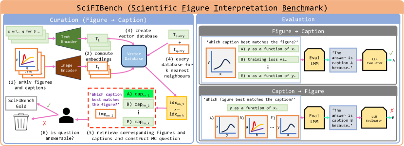
Figure 1: Overview of SciFIBench curation and tasks. Left: our benchmark gold dataset consists of 1000 multiple-choice scientific figure interpretation questions curated from arXiv papers using adversarial filtering and human verification to maximise difficulty and quality, respectively. Right: we evaluate a suite of LMMs on the two core SciFIBench tasks, leveraging an LLM for automatic evaluation.

1 Introduction

Lately, the rate of progress in the development of artificial intelligence (AI) has significantly increased. The emergence of foundation models [7], trained on large-scale broad data using extensive computational resources enabling generalisation across many downstream applications, has greatly expanded the range of possible domains and tasks in which machine intelligence can operate. Notable large language models (LLMs), such as GPT-4 [37], LLaMA [51], and PaLM [9], and subsequent large multimodal models (LMMs) , for example, GPT-4V [38], Qwen [6], and Gemini [49], have proven to be flexible and generalisable across many tasks. In particular, their capabilities have been demonstrated in fields such as mathematics [14, 64, 60], medicine [27, 54, 12, 24, 60], and finance [55, 59], as well as writing code [8] and the geographic and geospatial domains [44, 45].

One area that is beginning to receive more attention is the scientific domain, which has the potential to greatly benefit from AI tooling. Although the current generation of frontier models is arguably unable to perform independent, end-to-end scientific research, there is an emerging body of evidence [8, 60, 36, 3, 21, 4] suggesting they can be used as a tool to assist different stages of the scientific process. A key aspect of scientific research is the ability to understand figures, which serve as a rich, compressed source of complex information. As noted in [56], unique challenges arise from the complex and dense semantics of scientific images and the sophisticated language preferences of researchers. While the abilities of LMMs across some domains are relatively well-understood thanks to established benchmarks [65, 32, 33, 29, 28], their capacity to understand scientific figures is not well known. However, reliably characterising the ability of a model to interpret scientific figures is challenging without an obvious objective evaluation metric. Another consideration is the source of accurate ground truth; manually annotating a sufficiently large evaluation set of figures with accurate descriptions is unfeasible, and challenging without appropriate domain knowledge.

We circumvent these issues by reframing the evaluation to a multiple-choice setting, using the figure captions as ground truth descriptions – see Fig. 1. Concretely, using $\sim$100k figure-caption pairs from arXiv papers, we construct a pool of multiple-choice questions for the two tasks shown in Fig. 1. Following other popular works [66], we adopt adversarial filtering when curating the negatives for each question to increase the difficulty. To further improve the quality, we utilise human verification on every question to ensure they are maximally answerable. We create SciFIBench (Scientific Figure Interpretation Benchmark) by sampling from this question pool with the following three objectives in mind: (1) Quality – we perform human verification on every question to ensure high-quality questions that are answerable. (2) Efficiency – we choose a small-scale set of questions, enabling streamlined evaluation and ensuring the benchmark can maximally be used by the community. (3) Robustness – we conduct careful analysis to verify SciFIBench offers a suitably robust evaluation. Our benchmark includes a gold dataset consisting of 1000 questions, a silver dataset of 10k questions, and a bronze dataset consisting of 174k questions (see Tab. 1).

We evaluate a suite of 26 open- and closed-source LMM baselines on SciFIBench and compare the performance to human and vision-language model (VLM) baselines. To overcome the challenges associated with post-processing the output of LMMs to extract a specific answer at scale, we leverage Gemini-Pro [49] to parse the output of all evaluated LMMs and extract the relevant multiple-choice letter answers, enabling automatic evaluation. Finally, we carry out preliminary experiments probing the alignment and faithfulness of the LMMs when answering questions in our benchmark. We hope our insights will encourage further research in this direction.

To conclude, our main contributions are as follows: (i) We curate SciFIBench to evaluate scientific figure interpretation. (ii) We benchmark 26 LMMs on SciFIBench and compare the performance to human and VLM baselines. (iii) We introduce an experimental setting probing the instruction-following abilities and faithfulness of reasoning of the LMMs. (iv) We release SciFIBench to drive progress in LMM scientific figure interpretation and understanding research.

We derive these key insights from our work:

• SciFIBench proves to be a challenging benchmark for current LMMs.

• Closed-source LMMs outperform open-source models on our benchmark.

• GPT-4o [39] and Gemini-Pro 1.5 [43] are the best-performing models, outperforming all the VLM baselines but are beaten by the human baseline.

• Adversarial filtering significantly increases multiple-choice question difficulty but human filtering is crucial to ensure high-quality, answerable questions.

• Leveraging a strong LLM to evaluate the noisy output of the evaluated LMMs proves accurate and viable for automatic evaluation.

• The evaluated LMMs show varying levels of faithfulness in their answers.

2 Related Work

2.1 Scientific Figure Interpretation

Several approaches have been proposed to investigate the capacity of multimodal models to interpret scientific figures. These include question answering benchmarks such as ChartQA [34], PlotQA [35], and FigureQA [22], which ask complex reasoning questions about scientific figures. ACL-Fig [23] introduces the task of type classification for scientific figures. A large body of literature exists that evaluates the quality of generated captions for scientific figures. The progenitor for many subsequent works is SciCap [18], in which an image-captioning model is trained to generate high-quality captions. SciCap+ [61] builds this idea further and includes figure mention-paragraphs in addition to input figures. SciCap-Eval [19] investigates the usage of LLMs for ranking scientific figure captions. VisText [48] fine-tunes language models to generate captions for scientific charts, and FigCaps-HF [46] introduces a framework that initially learns a human feedback prediction model and incorporates this to optimise caption generation based on reader preference. The SciMMIR benchmark [56] characterises the abilities of vision-language models to understand scientific figures through retrieval experiments. More recently, a few works [38, 60] have conducted a qualitative analysis of LMM (specifically, GPT-4V [38]) performance on a small handful of scientific figures. We draw inspiration from these works, incorporating some of the methodological ideas. However, our work focuses on a quantitative evaluation of LMMs for the task of understanding scientific figures, which has yet to be reported. We also re-frame the task to a multiple-choice setting as this is more suitable for robust evaluation of LMMs.

2.2 LMM Benchmarks

A number of benchmarks aimed at multimodal model evaluation have been developed in recent years. Prominent natural image benchmarks include LVLM-eHub [58], MMBench [32], MME [16], MM-Vet [63], and SEEDBench [29] and SEEDBench-2 [28], which both consist of multiple-choice questions across different domains and evaluation dimensions. A small-scale geographic and geospatial benchmark is introduced in [45]. LAMM [62] evaluates a variety of computer vision tasks on 2D natural images as well as 3D point clouds. Other benchmarks, such as HallusionBench [17], focus on the failure modes and hallucinations of the models. MathVista [33] introduces a mathematical reasoning in visual contexts metadataset, which includes scientific figures and charts. This benchmark contains similar image types to our work but has a different focus and uses different question types. The MMMU benchmark [65] includes multi-discipline college-level image-based problems and questions. Although limited to text, we take inspiration by the adversarial filtering approach taken in [66], in the curation of the multiple-choice questions in our work. Our work incorporates stylistic and methodological inspiration from these works but tackles a different image type with a different overall focus of scientific figure interpretation.

3 SciFIBench

3.1 Overview

Overall, SciFIBench is comprised of $\sim$188k questions, derived from figures and captions extracted from arXiv papers, curated into two multiple-choice tasks. As illustrated in Tab. 1, we split our dataset into 3 subsets, each with different purposes. We focus on the high-quality gold set in our evaluation and benchmarking, and reserve the noisier silver and bronze subsets for downstream hyperparameter tuning, few-shot examples, or fine-tuning.

Split	# Questions		Human	Category	Difficulty
	Figure $\rightarrow$ Caption	Caption $\rightarrow$ Figure	curation?	balanced?
Bronze	87k	87k	✗	✗	Easy
Silver	5k	5k	✗	✓	Medium
Gold	500	500	✓	✓	Hard

Table 1: SciFIBench dataset splits.

3.2 Tasks

SciFIBench consists of the following two core tasks related to the interpretation of scientific figures (illustrated in Fig. 1):

Figure $\rightarrow$ Caption: Given an input figure, along with a set of 5 captions labeled A-E, select the correct caption for the figure.

Caption $\rightarrow$ Figure: Given an input caption, along with a set of 5 figures labeled A-E, select the correct figure for the caption.

3.3 Curation methodology

We use the SciCap dataset [18] as our source of scientific figure-caption pairs. SciCap is a large-scale dataset consisting of figures and corresponding captions extracted from arXiv computer science papers between the years 2010 - 2020.

From SciCap, we select the Single-Sentence subset (train, val, test), containing $\sim$94k figure-caption pairs, and only includes captions that are one sentence in length. The figures are filtered to remove any containing subfigures, and the captions are normalised to remove figure numbers. We then perform the following preprocessing and curation steps:

1. Deduplication: We initially drop any captions (and corresponding figures) if they are duplicates of other captions.

2. Compute embeddings: We then use a variant of the CLIP model [42] to compute embeddings for each figure-caption pair. After normalising, we concatenate the text and image embeddings to form joint embeddings, represented as vectors $x\in\mathbb{R}^{d}$, where $d$ is equal to 2048.

3. Construct vector database: Using the Faiss library [13], we create a vector database of the joint embeddings.

4. Find nearest neighbours: For each embedding, we search for the $k$ nearest neighbours based on Euclidean distance. Concretely, given the set of database embeddings $\{x_{i},i=1..N\}\subset\mathbb{R}^{d}$ and a query embedding $q\in\mathbb{R}^{d}$, we compute the $k$ nearest neighbours of $q$ as:

   $$(n_{1},\ldots,n_{k})=\underset{n=1..N}{\mathrm{argmin}^{k}}||q-x_{n}||.$$ (1)

5. Similarity filtering: To increase the likelihood the multiple-choice questions are answerable we remove very similar figure-caption pairs from our dataset (e.g., with minor formatting differences but no semantic difference) by dropping a sample ($x_{s}$) if its distance to the query embedding (i.e., $||q-x_{s}||$) falls below a threshold.

6. Question construction: For each selected figure-caption pair, we create multiple-choice questions using the $k$ nearest neighbours. For the Figure $\rightarrow$ Caption task, we create target captions by randomly shuffling the true caption with the corresponding $k$ nearest neighbour captions. Similarly, for the Caption $\rightarrow$ Figure task, we create the target figures by randomly shuffling the true figure with the corresponding $k$ nearest neighbour figures.

7. Categorisation: We categorise questions based on the arXiv category of the paper of the true figure-caption pair. Questions in the 10 most common categories are grouped individually while those in less common categories are labelled ‘other cs’; questions from cross-listed papers are labelled ‘cross-list’.

8. Difficulty filtering: For each question, we adopt the average distance score of the joint embeddings of the negatives to the true answer as a measure of difficulty. We sort the questions based on this difficulty.

9. Human verification: We sample the most difficult questions per category and perform human verification to select ‘answerable’ questions. We classify a question as answerable if it contains sufficient information for a domain expert to determine the single correct answer (i.e., questions with ambiguous choices; or references to context-dependent details, such as ‘Exp. 1’, ‘Config. 1’, etc. are disregarded). Minor text edits were made for a small subset of the questions to reduce ambiguity.

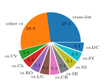
(a) Figure $\rightarrow$ Caption

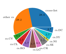
(b) Caption $\rightarrow$ Figure

Figure 2: SciFIBench gold set category representation.

Following these steps, we obtain a pool of high-quality answerable questions ($>$600 per task). We evaluate GPT-4V [38] and Gemini-Pro Vision [49] on the pool and select questions that either model answers incorrectly. Then, we sample the remaining questions per category to create the gold subset of 500 questions per task. Due to some categories having few answerable questions in the pool, category balance was approached, but not exactly achieved in all cases – Fig. 2 illustrates the category representation per task. For example, although the ‘cs.AI’ category is in the top 10 most common, the pool of possible questions was dominated by figures/captions from a single paper; to avoid introducing bias, we only included 10 such questions per task. The silver subset was then constructed by taking the next 5000 most difficult questions per task, sampled across categories, without human checking, and the bronze set was then formed of all remaining questions. Example gold set questions for each task are shown in Fig. 3. These examples demonstrate the increased difficulty introduced by adversarially selecting the negative multiple-choice answers relative to randomly selected choices. Another observation is that determining the correct answer for some questions requires interpreting fine-grained detail, especially in the figures (correctly answering the Caption $\rightarrow$ Figure example requires information in the figure legend).

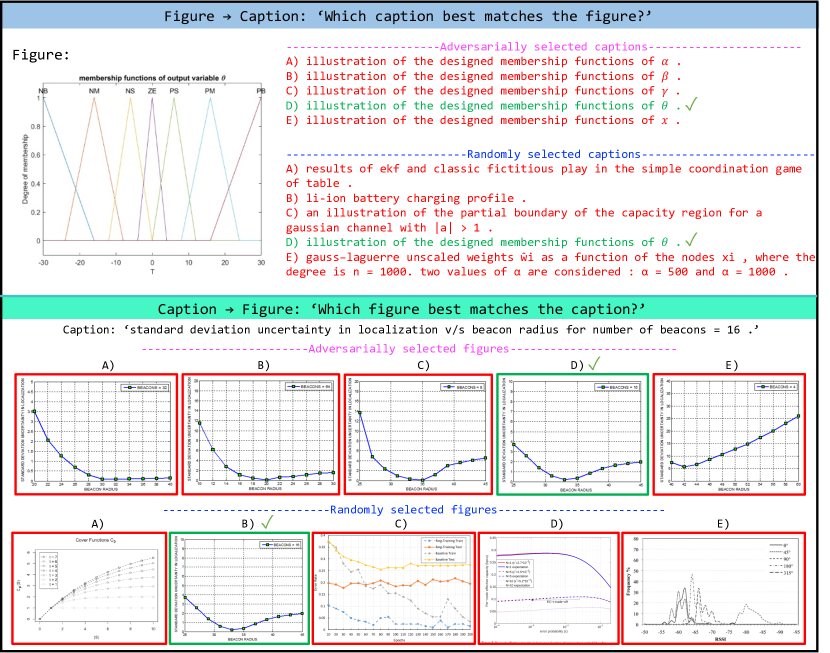
Figure 3: Example questions from our SciFIBench gold dataset. We show examples questions from each task and include both the challenging adversarially selected negatives and easier randomly selected negatives.

3.4 Quality control

A central motivation for focusing our evaluation on a small gold subset is to ensure high quality. As such, having manually checked each question, we conservatively estimate the noise level in the gold set to be at most a few percent. In these minority, questionable cases, we estimate there is a reasonable chance the questions can be answered with appropriate domain expertise. Based on spot checks, we estimate the noise level on the silver and bronze sets to be $\sim$20-25%. Across all sets, the noise rate is close to zero with randomly selected negatives.

Minor cosmetic errors, such as typos in captions or obscured axis labels, originating from the original SciCap data [18] were deliberately left unchanged when included in SciFIBench to increase question realism and difficulty.

3.5 Question difficulty

Preliminary ablation studies on a randomly sampled set of questions showed that, for nearly all the LMMs evaluated, finding hard negatives for each question using nearest neighbours determined based on the joint-embedding similarity yields the most challenging questions, with lower accuracy scores on the joint-embedding neighbours than the single-modality neighbours. Fig. 4 outlines the difficulty distribution of questions in the gold and silver subsets, based on $L_{2}$ distance. The effect of adversarially selecting negatives compared to random selection can be seen in the disparity of the orange and blue distributions, with the adversarial negatives having a much lower mean $L_{2}$ distance and therefore higher difficulty. As expected from the curation process, the gold adversarial distribution is more challenging than the silver distribution.

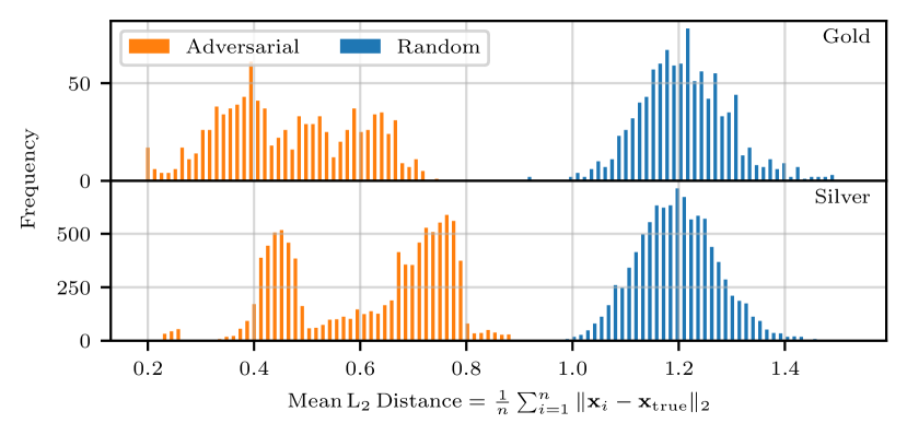
Figure 4: Difficulty distribution of questions in the Gold and Silver sets. We gauge difficulty using the mean L₂ distance between the embeddings (x) of the positive and negative answers for each question. A higher distance indicates an easier question.

4 Experiments

Through a variety of experiments, we evaluate the scientific figure interpretation abilities of a selection of closed- and open-source LMMs on our SciFIBench benchmark. We conduct our evaluations in a zero-shot setting and provide prompting and inference details in the following subsections. As it contains higher quality and more challenging questions, we focus our evaluation on the SciFIBench gold dataset.

4.1 Baselines

LMMs. In addition to the current frontier closed-source models (i) GPT-4V [38], (ii) GPT-4o [39] (iii) Gemini-Pro Vision [49], (iv) Gemini-Pro 1.5 [43], (v) Claude 3 {Opus, Sonnet and Haiku} [5], we evaluation the following open-source models on our benchmark: (vi) IDEFICS [26], (vii) Qwen-VL [6], (viii) Emu2 [47], (ix) TransCore-M [41], (x) InternLM-Composer [50], (xi) InternLM-Composer2 [50], (xii) CogVLM [52], (xiii) OmniLMM [40], (xiv) Yi [1], (xv) InstructBLIP [11], (xvi) Monkey [30], and (xvii) LLaVA-1.5 [31]. We use chat / instruction-tuned variants of each model (rather than base models) and compare the performance of multiple model sizes where available. Roughly half of these baselines can take interleaved text and images as input, and therefore be evaluated on the Caption$\rightarrow$Figure task.
VLMs. As a point of comparison, we also evaluate strong VLM models on SciFIBench. Specifically, we evaluate a MetaCLIP [57] variant, the Google Multimodal Embedding Model, and the CLIP model used to determine the nearest neighbour multiple-choice options.
Humans. Additionally, we evaluate a human baseline to gauge the relative performance difference between humans and LMMs. The humans (undergraduate and postgraduate students) were presented with the same prompt as the models.

While it is difficult to say with certainty if SciCap or arXiv data was included in the training sets of these models, there might be some leakage, as expected when using web images. However, given the scale of the training data, we do not expect this to impact our evaluation.

4.2 Experimental Settings

Inference. For the closed-source models, inference was carried out via the OpenAI API or Vertex AI API. We use the HuggingFace Transformers library [53] and OpenCompass toolkit [10] to access the open-source models and conduct inference using NVIDIA A100 GPUs. With current pricing, evaluating GPT-4V on the SciFIBench gold set costs $\sim$$15. For the open-source models, the typical gold set inference runtime using an A100 is $\sim$45 minutes (e.g., using Qwen-VL).

Hyperparameters. We select model hyperparameter settings that produce deterministic output to encourage reproducibility. For the open-source models, we utilise the greedy search decoding strategy, in which the most probable token is selected from the model vocabulary $V$ at each step, conditional on the preceding tokens i.e., $w_{n+1}=\arg\max_{w\in V}P(w|w_{1},w_{2},\ldots,w_{n})$. For the Gemini and Claude 3 models, we set the $temperature$ to 0 and $topk$ to 1; for the GPT-4 models, we also set the $temperature$ to 0 and specify a random seed.

Prompting. We adopt a generic 0-shot chain-of-thought [25] style prompt for each task, details of which can be found in the Appendix. Where relevant, we follow model-specific prompting suggestions and modify the prompt template accordingly. We found that shuffling the order of the multiple-choice answers causes performance to vary within a range of 5%.

Evaluation Metrics. We utilise a single evaluation metric when determining performance: the proportion of questions answered correctly. The same metric is used across both tasks.

Automatic Evaluation. Despite instruction in the prompt to constrain the format of the model answers to each question to just the target choice letter, e.g., ‘A’, most of the evaluated models did not consistently follow this, posing a challenge to automatic evaluation (string comparison). To overcome this, we used Gemini-Pro to initially parse the output and extract the answer letter or flag if no single answer was given.

4.3 Main Results

To gauge the abilities of frontier LMMs to interpret scientific figures, we evaluate a diverse set of LMMs and other baselines on our SciFIBench gold dataset, the results for which are displayed in Tab. 2. Note, our core analysis is in reference to results obtained on the adversarially generated question negatives (columns 2 and 4). We present our key findings as follows:

	Accuracy
Model	Figure$\rightarrow$Caption			Caption$\rightarrow$Figure
	Adversarial negatives		Random negatives	Adversarial negatives		Random negatives
Closed-source LMMs
GPT-4V [38]	69.4	+29.8	99.2	58.4	+38.0	96.4
GPT-4o [39]	75.4	+24.2	99.6	72.2	+26.8	99.0
Gemini-Pro Vision [49]	56.0	+41.2	97.2	52.4	+46.0	98.4
Gemini-Pro 1.5 [43]	74.0	+25.0	99.0	76.0	+22.4	98.4
Claude 3 Haiku [5]	52.6	+36.4	89.0	43.8	+34.6	78.4
Claude 3 Sonnet [5]	53.4	+33.0	86.4	58.4	+31.6	90.0
Claude 3 Opus [5]	59.8	+27.0	88.2	49.2	+32.0	81.2
Open-source LMMs
IDEFICS-9b-Instruct [26]	20.6	+4.4	25.0	20.2	-3.0	17.2
IDEFICS-80b-Instruct [26]	20.6	+17.6	38.2	24.2	+0.4	24.6
Qwen-VL-Chat [6]	28.0	+30.0	58.0	16.0	+1.0	17.0
Emu2 [47]	20.8	+28.4	49.2	-	-	-
TransCore-M [41]	51.0	+28.2	79.2	-	-	-
InternLM-XComposer-7b [50]	34.0	+21.6	55.6	-	-	-
InternLM-XComposer2-7b [50]	28.0	+46.0	74.0	-	-	-
CogVLM-Chat [52]	40.8	+17.0	57.8	-	-	-
OmniLMM-3b [40]	35.8	+29.0	64.8	-	-	-
OmniLMM-12b [40]	34.2	+34.0	68.2	-	-	-
Yi-VL-6b [1]	41.4	+30.4	71.8	-	-	-
Yi-VL-34b [1]	32.6	+29.4	62.0	-	-	-
InstructBLIP-FlanT5-xl [11]	35.8	+22.2	58.0	-	-	-
InstructBLIP-FlanT5-xxl [11]	36.2	+20.4	56.6	-	-	-
InstructBLIP-Vicuna-7b [11]	21.0	-3.4	17.6	-	-	-
InstructBLIP-Vicuna-13b [11]	22.2	+5.2	27.4	-	-	-
Monkey-Chat [30]	27.2	+22.8	50.0	-	-	-
LLaVA-1.5-7b [31]	32.8	+27.8	60.6	-	-	-
LLaVA-1.5-13b [31]	25.0	+41.2	66.2	-	-	-
VLMs
CLIP ViT-H-14-378-quickgelu [20]	41.8	+50.6	92.4	42.6	+53.4	96.0
MetaCLIP ViT-H-14-quickgelu [57]	36.6	+53.2	89.8	35.4	+54.8	90.2
Google Multimodal Embedding [2]	47.6	+46.2	93.8	54.4	+44.0	98.4
Human (25 questions per task*)
Human ($\mu\pm{\color[rgb]{0.5,0.5,0.5}\sigma}$)	86.4$\pm$8.24	+10.7	100.0	78.4$\pm$8.24	+22.7	100.0
GPT-4o	72.0	+28.0	100.0	76.0	+24.0	100.0
Gemini-Pro 1.5	84.0	+16.0	100.0	72.0	+28.0	100.0
Claude 3 Opus	72.0	+8.0	80.0	56.0	+32.0	88.0
GPT-4V	68.0	+28.0	96.0	56.0	+40.0	96.0
CLIP ViT-H-14-378-quickgelu	48.0	+44.0	92.0	56.0	+44.0	100.0
TransCore-M	36.0	+48.0	84.0	-	-	-

Table 2: Performance on the SciFIBench gold dataset. Results for questions with adversarially-selected negatives and randomly-selected negatives are shown, along with the difference between them. ^∗25 questions per task were randomly selected for the human baseline experiments with model scores shown for the same subset of questions. For the adversarial negatives setting, the human score is calculated as a mean of 5 participants, while only one human conducted the random negatives evaluation.

SciFIBench represents a difficult benchmark. The best-performing models, GPT-4o and Gemini-Pro 1.5, attain scores of 75.4% and 74.0% for the Figure $\rightarrow$ Caption task, respectively, and 72.2% and 76.0% for the Caption $\rightarrow$ Figure tasks, respectively. This shows that even at the frontier there is sufficient headroom for improvement. Among the weaker models, there is much more headroom, with the weakest models only just equalling or barely surpassing the chance score. Overall, there is a large spread of performance scores across the models, suggesting the benchmark has a good range of question difficulties.
Closed-source models are noticeably better than open-source models. We observe a large performance gap between the closed-source and open-source models. Considering the Figure $\rightarrow$ Caption task, there is a difference of 24.4% between the scores of the best closed and open-sourced models. Moreover, the best-performing open-source model, TransCore-M underperforms the worst-performing closed-source model, Claude 3 Haiku. This difference is more pronounced for the Caption $\rightarrow$ Figure task.
Adversarially selected negatives are more challenging. As an ablation, we compare model performance when answering questions with adversarially selected multiple-choice negatives and randomly selected negatives (see Tab. 2 coloured text). As expected, in the vast majority of cases, accuracy scores are higher on the random negatives – for some open-source models, the accuracy score more than doubles, and for the closed-source models, the maximum accuracy score is almost met. However, for the open-source models evaluated on the Caption $\rightarrow$ Figure task, there is almost no change in performance between the adversarial and random negative settings. Given that the scores are close to the chance score, it is likely this task is too challenging for these models.
Caption $\rightarrow$ Figure is more difficult than Figure $\rightarrow$ Caption. Among the closed-source models, slightly higher overall scores are attained on the Figure $\rightarrow$ Caption task. This observation holds for the open-source models, especially in the random negatives setting. Considering the human baseline, a noticeably lower score is attained on the Caption $\rightarrow$ Figure task, suggesting it is easier for humans to distinguish fine-grained details in the text domain. The VLM baselines show no discernible difference in performance across the tasks, a possible reflection of their pretraining strategy of jointly aligning language and vision.
Performance does not necessarily scale with model size. Considering the models that we evaluate different checkpoint sizes (i.e., IDEFICS, OmniLMM, Yi, InstructBLIP-FlanT5, InstructBLIP-Vicuna, LLaVA-1.5, InternLM), we find that more often than not, the smaller model outperforms the larger checkpoint on the adversarially selected negatives, however, the opposite is true for the randomly selected negatives. Additionally, the difference in performance is more pronounced on the randomly selected negatives.
CLIP remains a strong baseline. Across both tasks, on questions with adversarial negatives, the CLIP baseline performs comparably or superior to the leading open-source models, though is beaten by the closed-source models. When negatives are randomly selected, CLIP far surpasses the open-source models, almost equalling GPT-4V and the Gemini-Pro models.
Humans are a stronger baseline. The mean human baseline outperforms all the models, though does not achieve a perfect score, reflecting the challenging nature of this benchmark and the fact that the participants were not necessarily domain experts. As indicated by the standard deviation, a range of accuracy scores were recorded for each task, with some participants scoring equal or lower than the best LMMs. It is worth noting a slight caveat to the human performance is that the human verification part of the dataset curation process could have introduced bias toward questions that are ‘easier’ for humans to answer.

In the Appendix, we include qualitative results for each task and examples of model output before automatic evaluation.

4.4 Performance Across Categories

We analyse the performance of a representative sample of models on the Figure $\rightarrow$ Caption task across the 12 categories in the SciFIBench gold dataset. The results are displayed in Fig. 5 and comprehensive results for all models can be found in the Appendix. Although the different categories in our benchmark are all (at least partly) from the arXiv CS category, there is considerable variation in the style and type of figures within each category. This disparity is reflected in the difference in performance across categories: the average accuracy for the selected models differs by 22.5% between the best category (LG) and the worse category (AI). There is slight variation in ranking of the models across categories, but it remains fairly consistent.

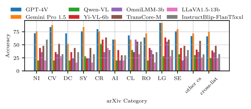
Figure 5: Performance variation across question categories for selected models on the Figure $\rightarrow$ Caption task of the gold dataset.

4.5 Gold vs. Silver Datasets

Due to its increased quality and feasibility of evaluation, our analysis is focused on the gold set, with our main intentions for the silver and bronze sets being downstream fine-tuning and few-shot evaluation. Here, we justify this decision and provide evidence that although our gold set is relatively small, it is sufficiently robust. We evaluate a subset of our models on both the gold and silver sets and plot their relative rankings in Fig. 6. For almost all models, the ranking is preserved across the datasets, and in the case where the rankings switch, the performance differential between the two models is small. A key purpose of a benchmark is to provide the rankings of models. This analysis shows that this indicator is largely sustained, suggesting there is little information to be gained by evaluating on an arbitrarily larger dataset. Moreover, we conduct bootstrapping to estimate the variance of model performance on the gold dataset (500 questions for each task). Concretely, for each task, we sample with replacement 500 times from the relevant question set and evaluate the performance of Gemini Pro Vision (middle-performing model capable of both tasks) on the sample. Repeating this process 100k times yields a mean accuracy and variance of (56.00, 0.05) and (52.40, 0.05) for the Figure $\rightarrow$ Caption and Caption $\rightarrow$ Figure tasks, respectively. This low variance provides further evidence that our gold dataset is sufficiently representative.

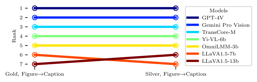
Figure 6: Performance ranking comparison of models evaluated on the gold and silver datasets. We observe only minor variations in raking between the small, high-quality dataset and larger, noisy dataset.

4.6 Alignment

A central motivation of this work is guiding the progress of LMMs to conduct scientific research. However, if LMMs are to be utilised as a tool for scientific acceleration and discovery, it is not sufficient to simply evaluate their performance, it is crucial to ensure they are aligned and the degree to which they can reliably follow instructions is known. To this end, we devise a small-scale experiment to probe this instruction-following ability and see if the models reason faithfully or are prone to ‘cheating’. In addition to a control baseline, we create 4 different augmentations of the gold dataset Figure $\rightarrow$ Caption questions. Illustration of the augmentations are shown in Fig. 7. In two of the augmentations, we mark the true caption as <Correct>. In one of these, we additionally instruct the model to ignore this extra information. For the remaining two augmentations, we repeat this process, however, we mark a randomly chosen incorrect caption as <Correct>. We evaluate the performance accuracy on each augmented question set for a representative selection of LMMs and display the results in Fig. 8.

Annotating an answer as correct significantly changes performance. We find that for all models, marking the correct answer has a noticeable increase in performance relative to the baseline. Similarly, marking the incorrect answer as correct consistently decreases the performance relative to the baseline. There are also clear differences in sensitivity to this new information. For example, the performance relative to the baseline for Qwen-VL and Gemini-Pro Vision varies at most 30%, whereas for models like LLaVA-1.5 and OmniLMM, the difference exceeds 50%.

Some models are better at following instructions. We can obtain a gauge of the alignment of the models by analysing the degree to which instruction to ignore the <Correct> annotation is followed. In almost every case, we find that the instruction does cause the performance to change in the desired direction (i.e., towards the baseline score), though the amount of change varies depending on the model. For example, the performance of OmniLMM and TransCore-M shows almost no difference when instructed to ignore the annotation, suggesting weaker instruction-following. Whereas, the performance of CogVLM in particular changes drastically with the additional instruction.

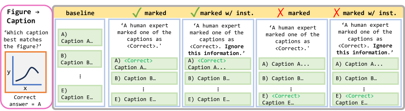
Figure 7: Alignment experiment overview. We create 4 augmentations of the baseline Figure $\rightarrow$ Caption questions with different information and instructions.

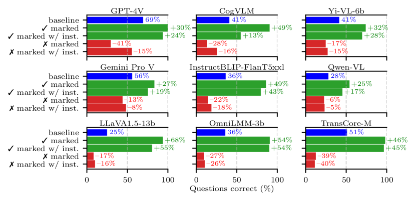
Figure 8: Performance comparison on the augmented question sets. Note, the labelled percentage changes reflect the change in accuracy relative to the baseline.

5 Conclusions

We introduce the Scientific Figure Interpretation Benchmark (SciFIBench) to evaluate the capabilities of LMMs to interpret and understand scientific figures. We curate the multiple-choice questions in our benchmark using arXiv paper figure-captions pairs from the SciCap dataset [18] and employ adversarial filtering to select hard negatives, increasing the difficulty of our benchmark. We use human verification when selecting questions to construct a robust, high-quality dataset that can be used to efficiently evaluate future models without the need for extensive compute or API credits. We benchmark the performance of 30 LMM, VLM and human baselines on SciFIBench, finding it to be challenging, with room for improvement. Finally, we analyse the alignment and instruction following abilities of the LMMs when answering questions in our benchmark. We release our dataset for the community to use and hope our work encourages further research in this important domain.

Appendix

We structure this Appendix to our main paper into four parts. First, we include the API model names/versions used in our evaluation (Sec. A). Next, we provide details of the prompt templates used for the two tasks that make up SciFIBench (Sec. B). Then, we provide additional experimental results, including human baseline details, and full results tables for Fig 5 that include evaluation on more models (Sec. C). Finally, we demonstrate qualitative results on SciFIBench including example questions along with LMM (large multimodal model) output and reasoning, and we additionally provide examples of the LMM output before and after automatic evaluation (Sec. D). To improve clarity, in this Appendix we format model inputs (e.g., prompts) as and model outputs as .

A API model versions

These are the specific versions of the API models used in this work:

• GPT-4V: gpt-4-vision-preview

• GPT-4o: gpt-4o-2024-05-13

• Gemini-Pro Vision: gemini-pro-vision

• Gemini-Pro: gemini-1.0-pro-001

• Gemini-Pro 1.5: gemini-1.5-pro-preview-0409

• Claude 3 Opus: claude-3-opus@20240229

• Claude 3 Sonnet: claude-3-sonnet@20240229

• Claude 3 Haiku: claude-3-haiku@20240307

B Prompt templates

B.1 Task prompts

Below, we include the prompt templates used in the Figure $\rightarrow$ Caption task and Caption $\rightarrow$ Figure task. These prompt templates were utilised by each model, however, in some cases minor modifications were implemented depending on prompting suggestions mentioned by model authors. Note, items in parenthesis – e.g., {Caption} or {Image} – represent the placement of the actual image or caption within the prompt.

Figure $\rightarrow$ Caption

Caption $\rightarrow$ Figure

B.2 Automatic evaluation

We use the following when prompting Gemini-Pro to automatically evaluate the output of all LMMs.

See Figs. 9 and 10 for examples of LMM output before and after reformatting with Gemini-Pro using the above prompt.

C Extended quantitative results

C.1 Human baseline

The individual results for the human baseline are included below in Tab. 3. The questions were randomly sampled from the SciFIBench gold dataset (using adversarial negatives) and evaluated by 5 humans (comprising both undergraduate and postgraduate students).

Human/Model	Accuracy
	Figure $\rightarrow$ Caption	Caption $\rightarrow$ Figure
Human 1	96.0	92.0
Human 2	88.0	68.0
Human 3	84.0	72.0
Human 4	72.0	80.0
Human 5	92.0	80.0
Mean Human	86.4	78.4
GPT-4o	72.0	76.0
Gemini-Pro 1.5	84.0	72.0

Table 3: Extended human baseline results. Human baseline accuracy on a 25 question-per-task subset of SciFIBench gold dataset. The best score for each task is in bold. Results on the same question set for the leading LMMs (GPT-4o and Gemini-Pro 1.5) are included as a comparison.

Several observations can be drawn from these results: (1) Human variance – Across both tasks, there is a high degree of variance on the accuracy scores of the different humans that answered the questions. (2) Comparison to closed-source models – Across most axes, the ranking of the human baseline above the leading LMM baselines (GPT-4o and Gemini-Pro 1.5) outlined in the main paper is preserved. Although on each task there are some humans that are outperformed by at least one of the LMMs, the mean human beats the LMMs, which are also either beaten or equalled by the median human.

It is worth acknowledging that this comparison to the human baseline has limitations. Firstly, this is a small sample that is not necessarily representative of the entire population, yet still has considerable variance. Another consideration is the learning that could occur during the question answering. Unlike the models, which answer each question independently, the humans answered the questions as part of a survey of 50 questions (25 per task). Although feedback was not given, it is possible, for example, that exposure to earlier questions influenced the approach taken to answering later questions.

C.2 Full per category results

In Tab. 4 below, we include full results for the per-category performance on the Figure $\rightarrow$ Caption task of the SciFIBench gold dataset. This table expands on Fig. 5 in the main paper by including scores for each model displayed in the graph, as well as results for additional models evaluated.

Model	Accuracy per category
	cs.NI	cs.CV	cs.DC	cs.SY	cs.CR	cs.AI	cs.CL	cs.RO	cs.LG	cs.SE	other cs	cross-list	Total
GPT-4V	72.0	84.0	64.0	76.0	80.0	60.0	72.0	68.0	88.0	68.0	66.7	63.2	69.2
GPT-4o	76.0	84.0	64.0	80.0	92.0	20.0	68.0	76.0	96.0	72.0	71.2	78.2	75.4
Gemini-Pro Vision	48.0	76.0	56.0	56.0	96.0	10.0	56.0	32.0	76.0	64.0	56.1	48.9	56.0
Gemini-Pro 1.5	76.0	88.0	52.0	84.0	76.0	60.0	60.0	72.0	92.0	80.0	72.0	75.2	74.2
Claude 3 Haiku	48.0	56.0	44.0	60.0	76.0	20.0	64.0	64.0	48.0	56.0	52.3	47.4	52.6
Claude 3 Sonnet	64.0	68.0	40.0	64.0	76.0	60.0	48.0	52.0	68.0	60.0	46.2	48.9	53.4
Claude 3 Opus	56.0	60.0	44.0	64.0	80.0	30.0	64.0	68.0	76.0	56.0	59.8	57.1	60.0
IDEFICS-9b-Instruct	4.0	32.0	24.0	20.0	12.0	20.0	16.0	24.0	44.0	12.0	18.9	21.8	20.6
IDEFICS-80b-Instruct	16.0	28.0	20.0	24.0	20.0	20.0	0.0	12.0	4.0	20.0	28.0	21.1	20.6
Qwen-VL-Chat	20.0	20.0	20.0	28.0	52.0	20.0	40.0	20.0	28.0	32.0	30.3	24.8	28.0
Emu2-Chat	12.0	32.0	20.0	16.0	40.0	20.0	20.0	8.0	20.0	36.0	21.2	17.3	20.8
TransCore-M	48.0	52.0	44.0	44.0	64.0	30.0	56.0	32.0	60.0	48.0	57.6	48.1	51.0
InternLM-XComposer-7b	32.0	40.0	44.0	40.0	32.0	50.0	40.0	32.0	44.0	36.0	25.8	34.6	34.0
InternLM-XComposer2-7b	16.0	24.0	20.0	28.0	40.0	20.0	20.0	36.0	36.0	40.0	40.9	14.3	28.0
CogVLM-Chat	40.0	32.0	48.0	40.0	44.0	20.0	40.0	40.0	56.0	52.0	40.2	38.3	40.8
OmniLMM-3b	36.0	32.0	24.0	24.0	36.0	20.0	60.0	40.0	56.0	20.0	36.4	35.3	35.8
OmniLMM-12b	40.0	40.0	32.0	40.0	56.0	20.0	52.0	32.0	40.0	36.0	34.8	23.3	34.2
Yi-VL-6b	44.0	36.0	36.0	24.0	60.0	40.0	36.0	44.0	64.0	44.0	40.9	39.1	41.4
Yi-VL-34b	32.0	44.0	20.0	20.0	48.0	10.0	32.0	28.0	60.0	40.0	31.1	30.1	32.6
InstructBLIP-FlanT5-xl	32.0	28.0	32.0	48.0	40.0	50.0	44.0	48.0	36.0	40.0	32.6	33.1	35.8
InstructBLIP-FlanT5-xxl	60.0	32.0	36.0	32.0	40.0	30.0	56.0	36.0	40.0	40.0	31.8	32.3	36.2
InstructBLIP-Vicuna-7b	16.0	32.0	20.0	28.0	24.0	30.0	12.0	28.0	24.0	16.0	18.9	20.3	21.0
InstructBLIP-Vicuna-13b	24.0	16.0	24.0	24.0	36.0	10.0	28.0	16.0	8.0	28.0	21.2	23.3	22.2
Monkey-Chat	16.0	20.0	12.0	28.0	56.0	20.0	48.0	20.0	16.0	28.0	32.6	22.6	27.2
LLaVA-1.5-7b	20.0	32.0	44.0	32.0	56.0	10.0	48.0	28.0	32.0	12.0	30.3	35.3	32.8
LLaVA-1.5-13b	20.0	28.0	16.0	16.0	44.0	20.0	32.0	16.0	28.0	28.0	25.8	24.1	25.0
CLIP ViT-H-14-378-quickgelu	40.0	52.0	32.0	32.0	52.0	20.0	64.0	32.0	64.0	32.0	40.2	40.6	41.8
MetaCLIP ViT-H-14-quickgelu	28.0	44.0	20.0	32.0	48.0	10.0	56.0	48.0	32.0	44.0	39.4	31.6	36.6
Google Multimodal Embedding	36.0	72.0	16.0	36.0	56.0	20.0	76.0	56.0	68.0	60.0	44.7	43.6	47.6
Total	37.0	44.3	33.7	39.3	52.8	26.6	45.0	38.1	48.6	41.7	39.6	37.1	39.9

Table 4: Full-per category performance on the SciFIBench gold dataset, Figure $\rightarrow$ Caption task.

D Qualitative results

In this section, we present qualitative results to complement the quantitative results included in the main paper and show additional example SciFIBench questions. We structure these results in the following way: (1) Automatic postprocessing – For selected questions, we provide examples (Figs. 9-10) of both the raw output from a selection of the LMMs evaluated, and the formatted output following automatic answer extraction by Gemini-Pro. (2) Model reasoning – For a number of example questions (Figs. 11-16), we provide the reasoning steps taken by the models when producing an answer.

D.1 1. Automatic postprocessing

In Figs. 9 and 10 we provide examples of LMM output before and after automatic evaluation by Gemini-Pro. The examples show that Gemini-Pro is able to extract the correct prediction from the unformatted LMM output, greatly aiding automatic evaluation. For most models, only minor output formatting is required as the correct letter answer is given at the start of the output. However in some cases, such as the output of CogVLM in Fig 10, which begins: ‘The correct caption that best describes the image is:…’, this is not the case and more involved reasoning is required to extract the correct answer choice.

Figure $\rightarrow$ Caption: Which of the captions best describes the image? Image:

Model outputs:

Model	Raw output	Gemini-Pro output	Answer correct?
GPT-4V [38]			✓
Gemini-Pro Vision [49]			✓
CogVLM [52]			✓
Yi-VL-6B [1]			✗
Qwen-VL [6]			✗
OmniLMM-3B [40]			✗
TransCore-M [41]			✗
LLaVA-1.5-13b [27]			✗

Figure 9: Example of automatic output evaluation by Gemini-Pro. The example includes: (1) a randomly selected question from the SciFIBench gold dataset, Figure $\rightarrow$ Caption task; and, (2) Example LMM outputs before (raw) and after answer extraction by Gemini-Pro. [Note, the correct answer is D)].

Figure $\rightarrow$ Caption: Which of the captions best describes the image? Image:

Model outputs:

Model	Raw output	Gemini-Pro output	Answer correct?
GPT-4V [38]			✓
Gemini-Pro Vision [49]			✗
CogVLM [52]			✓
Yi-VL-6B [1]			✓
Qwen-VL [6]			✗
OmniLMM-3B [40]			✗
TransCore-M [41]			✗
LLaVA-1.5-13b [27]			✗

Figure 10: Another example of automatic output evaluation by Gemini-Pro. The example includes: (1) a randomly selected question from the SciFIBench gold dataset, Figure $\rightarrow$ Caption task; and, (2) Example LMM outputs before (raw) and after answer extraction by Gemini-Pro. [Note, the correct answer is E)].

D.2 2. Model reasoning

In the following subsection, we provide a series of qualitative examples of LMM reasoning when answering questions from the SciFIBench gold dataset. Specifically, we amend the prompts given in Sec. B to the following:

Figure $\rightarrow$ Caption

Caption $\rightarrow$ Figure

i.e., allowing the models to outline their reasoning steps by removing the output format constraint:

We structure each of the following examples as (i) Question – showing the question figure(s) and caption(s); and (ii) Outputs – showing the outputs from a selection of the LMMs evaluated. We provide examples for the Figure $\rightarrow$ Caption task (Figs. 11-14) and for the Caption $\rightarrow$ Figure task (Figs. 15-16).

Example 1: Figure $\rightarrow$ Caption – Which of the captions best describes the figure? Figure:

Figure 11: Example Figure $\rightarrow$ Caption question. [Note, the correct answer is A].

Model outputs:

GPT-4V:

Gemini-Pro Vision:

Qwen VL:

OmniLMM-3B:

TransCore-M:

LLaVA-1.5-13b:

Yi-VL-6b:

IDEFICS-9b-instruct:

CogVLM:

Example 2: Figure $\rightarrow$ Caption – Which of the captions best describes the figure? Figure:

Figure 12: Example Figure $\rightarrow$ Caption question. [Note, the correct answer is E)].

Model outputs:

GPT-4V:

Gemini-Pro Vision:

Qwen VL:

OmniLMM-3B:

TransCore-M:

LLaVA-1.5-13b:

Yi-VL-6b:

IDEFICS-9b-instruct:

CogVLM:

Example 3: Figure $\rightarrow$ Caption – Which of the captions best describes the figure? Figure:

Figure 13: Example Figure $\rightarrow$ Caption question. [Note, the correct answer is E)].

Model outputs:

GPT-4V:

Gemini-Pro Vision:

Qwen VL:

OmniLMM-3B:

TransCore-M:

LLaVA-1.5-13b:

Yi-VL-6b:

IDEFICS-9b-instruct:

CogVLM:

Example 4: Figure $\rightarrow$ Caption – Which of the captions best describes the figure? Figure:

Figure 14: Example Figure $\rightarrow$ Caption question. [Note, the correct answer is C)].

Model outputs:

GPT-4V:

Gemini-Pro Vision:

Qwen VL:

OmniLMM-3B:

TransCore-M:

LLaVA-1.5-13b:

Yi-VL-6b:

IDEFICS-9b-instruct:

CogVLM:

Example 5: Caption $\rightarrow$ Figure – Which of the figures best describes the caption?

A)

B)

C)

D)

E)

Figure 15: Example Caption $\rightarrow$ Figure question. [Note, the correct answer is E)].

Model outputs:

GPT-4V:

Gemini-Pro Vision:

Example 6: Caption $\rightarrow$ Figure – Which of the figures best describes the caption?

A)

B)

C)

D)

E)

Figure 16: Example Caption $\rightarrow$ Figure question. [Note, the correct answer is E)].

Model outputs:

GPT-4V:

Gemini-Pro Vision:

References

- [1] 01-ai: Yi. https://https://github.com/01-ai/Yi (2023)
- [2] AI, G.V.: Google Vertex AI MM Embedding Model (May 2024), https://console.cloud.google.com/vertex-ai/publishers/google/model-garden/multimodalembedding
- [3] AI4Science, M.R., Quantum, M.A.: The Impact of Large Language Models on Scientific Discovery: a Preliminary Study using GPT-4 (2023)
- [4] Almarie, B., Teixeira, P.E., Pacheco-Barrios, K., Rossetti, C.A., Fregni, F.: Editorial–The Use of Large Language Models in Science: Opportunities and Challenges. Principles and practice of clinical research (2015) 9(1), 1 (2023)
- [5] Anthropic: Introducing the next generation of Claude (Mar 2024), https://www.anthropic.com/news/claude-3-family
- [6] Bai, J., Bai, S., Yang, S., Wang, S., Tan, S., Wang, P., Lin, J., Zhou, C., Zhou, J.: Qwen-VL: A frontier large vision-language model with versatile abilities. arXiv preprint arXiv:2308.12966 (2023)
- [7] Bommasani, R., Hudson, D.A., Adeli, E., Altman, R., Arora, S., von Arx, S., Bernstein, M.S., Bohg, J., Bosselut, A., Brunskill, E., et al.: On the opportunities and risks of foundation models. arXiv preprint arXiv:2108.07258 (2021)
- [8] Bubeck, S., Chandrasekaran, V., Eldan, R., Gehrke, J., Horvitz, E., Kamar, E., Lee, P., Lee, Y.T., Li, Y., Lundberg, S., et al.: Sparks of artificial general intelligence: Early experiments with GPT-4. arXiv preprint arXiv:2303.12712 (2023)
- [9] Chowdhery, A., Narang, S., Devlin, J., Bosma, M., Mishra, G., Roberts, A., Barham, P., Chung, H.W., Sutton, C., Gehrmann, S., Schuh, P., Shi, K., Tsvyashchenko, S., Maynez, J., Rao, A., Barnes, P., Tay, Y., Shazeer, N., Prabhakaran, V., Reif, E., Du, N., Hutchinson, B., Pope, R., Bradbury, J., Austin, J., Isard, M., Gur-Ari, G., Yin, P., Duke, T., Levskaya, A., Ghemawat, S., Dev, S., Michalewski, H., Garcia, X., Misra, V., Robinson, K., Fedus, L., Zhou, D., Ippolito, D., Luan, D., Lim, H., Zoph, B., Spiridonov, A., Sepassi, R., Dohan, D., Agrawal, S., Omernick, M., Dai, A.M., Pillai, T.S., Pellat, M., Lewkowycz, A., Moreira, E., Child, R., Polozov, O., Lee, K., Zhou, Z., Wang, X., Saeta, B., Diaz, M., Firat, O., Catasta, M., Wei, J., Meier-Hellstern, K., Eck, D., Dean, J., Petrov, S., Fiedel, N.: PaLM: Scaling Language Modeling with Pathways (2022)
- [10] Contributors, O.: OpenCompass: A Universal Evaluation Platform for Foundation Models. https://github.com/open-compass/opencompass (2023)
- [11] Dai, W., Li, J., Li, D., Tiong, A.M.H., Zhao, J., Wang, W., Li, B., Fung, P., Hoi, S.: InstructBLIP: Towards General-purpose Vision-Language Models with Instruction Tuning (2023)
- [12] Dash, D., Thapa, R., Banda, J.M., Swaminathan, A., Cheatham, M., Kashyap, M., Kotecha, N., Chen, J.H., Gombar, S., Downing, L., et al.: Evaluation of GPT-3.5 and GPT-4 for supporting real-world information needs in healthcare delivery. arXiv preprint arXiv:2304.13714 (2023)
- [13] Douze, M., Guzhva, A., Deng, C., Johnson, J., Szilvasy, G., Mazaré, P.E., Lomeli, M., Hosseini, L., Jégou, H.: The Faiss library. arXiv preprint arXiv:2401.08281 (2024)
- [14] Driess, D., Xia, F., Sajjadi, M.S., Lynch, C., Chowdhery, A., Ichter, B., Wahid, A., Tompson, J., Vuong, Q., Yu, T., et al.: Palm-e: An embodied multimodal language model. arXiv preprint arXiv:2303.03378 (2023)
- [15] Fang, A., Jose, A.M., Jain, A., Schmidt, L., Toshev, A., Shankar, V.: Data filtering networks. arXiv preprint arXiv:2309.17425 (2023)
- [16] Fu, C., Chen, P., Shen, Y., Qin, Y., Zhang, M., Lin, X., Yang, J., Zheng, X., Li, K., Sun, X., et al.: Mme: A comprehensive evaluation benchmark for multimodal large language models. arXiv preprint arXiv:2306.13394 (2023)
- [17] Guan, T., Liu, F., Li, X.W.R.X.Z., Wang, X.L.X., Yacoob, L.C.F.H.Y., Zhou, D.M.T.: HALLUSIONBENCH: An Advanced Diagnostic Suite for Entangled Language Hallucination & Visual Illusion in Large Vision-Language Models. arXiv e-prints pp. arXiv–2310 (2023)
- [18] Hsu, T.Y., Giles, C.L., Huang, T.H.: SciCap: Generating captions for scientific figures. arXiv preprint arXiv:2110.11624 (2021)
- [19] Hsu, T.Y., Huang, C.Y., Rossi, R., Kim, S., Giles, C.L., Huang, T.H.K.: GPT-4 as an Effective Zero-Shot Evaluator for Scientific Figure Captions. arXiv preprint arXiv:2310.15405 (2023)
- [20] Ilharco, G., Wortsman, M., Wightman, R., Gordon, C., Carlini, N., Taori, R., Dave, A., Shankar, V., Namkoong, H., Miller, J., Hajishirzi, H., Farhadi, A., Schmidt, L.: OpenCLIP (Jul 2021). https://doi.org/10.5281/zenodo.5143773, https://doi.org/10.5281/zenodo.5143773
- [21] Jablonka, K.M., Ai, Q., Al-Feghali, A., Badhwar, S., Bocarsly, J.D., Bran, A.M., Bringuier, S., Brinson, L.C., Choudhary, K., Circi, D., et al.: 14 examples of how LLMs can transform materials science and chemistry: a reflection on a large language model hackathon. Digital Discovery 2(5), 1233–1250 (2023)
- [22] Kahou, S.E., Michalski, V., Atkinson, A., Kádár, Á., Trischler, A., Bengio, Y.: Figureqa: An annotated figure dataset for visual reasoning. arXiv preprint arXiv:1710.07300 (2017)
- [23] Karishma, Z., Rohatgi, S., Puranik, K.S., Wu, J., Giles, C.L.: ACL-Fig: A Dataset for Scientific Figure Classification. arXiv preprint arXiv:2301.12293 (2023)
- [24] Kasai, J., Kasai, Y., Sakaguchi, K., Yamada, Y., Radev, D.: Evaluating GPT-4 and ChatGPT on Japanese medical licensing examinations. arXiv preprint arXiv:2303.18027 (2023)
- [25] Kojima, T., Gu, S.S., Reid, M., Matsuo, Y., Iwasawa, Y.: Large Language Models are Zero-Shot Reasoners (2023)
- [26] Laurençon, H., Saulnier, L., Tronchon, L., Bekman, S., Singh, A., Lozhkov, A., Wang, T., Karamcheti, S., Rush, A.M., Kiela, D., Cord, M., Sanh, V.: OBELICS: An Open Web-Scale Filtered Dataset of Interleaved Image-Text Documents (2023)
- [27] Lee, S., Youn, J., Kim, M., Yoon, S.H.: CXR-LLaVA: Multimodal Large Language Model for Interpreting Chest X-ray Images (2023)
- [28] Li, B., Ge, Y., Ge, Y., Wang, G., Wang, R., Zhang, R., Shan, Y.: SEED-Bench-2: Benchmarking Multimodal Large Language Models (2023)
- [29] Li, B., Wang, R., Wang, G., Ge, Y., Ge, Y., Shan, Y.: SEED-Bench: Benchmarking Multimodal LLMs with Generative Comprehension (2023)
- [30] Li, Z., Yang, B., Liu, Q., Ma, Z., Zhang, S., Yang, J., Sun, Y., Liu, Y., Bai, X.: Monkey: Image Resolution and Text Label Are Important Things for Large Multi-modal Models. arXiv preprint arXiv:2311.06607 (2023)
- [31] Liu, H., Li, C., Li, Y., Lee, Y.J.: Improved Baselines with Visual Instruction Tuning (2023)
- [32] Liu, Y., Duan, H., Zhang, Y., Li, B., Zhang, S., Zhao, W., Yuan, Y., Wang, J., He, C., Liu, Z., et al.: Mmbench: Is your multi-modal model an all-around player? arXiv preprint arXiv:2307.06281 (2023)
- [33] Lu, P., Bansal, H., Xia, T., Liu, J., Li, C., Hajishirzi, H., Cheng, H., Chang, K.W., Galley, M., Gao, J.: Mathvista: Evaluating mathematical reasoning of foundation models in visual contexts. arXiv preprint arXiv:2310.02255 (2023)
- [34] Masry, A., Long, D.X., Tan, J.Q., Joty, S., Hoque, E.: ChartQA: A benchmark for question answering about charts with visual and logical reasoning. arXiv preprint arXiv:2203.10244 (2022)
- [35] Methani, N., Ganguly, P., Khapra, M.M., Kumar, P.: Plotqa: Reasoning over scientific plots. In: Proceedings of the IEEE/CVF Winter Conference on Applications of Computer Vision. pp. 1527–1536 (2020)
- [36] Nejjar, M., Zacharias, L., Stiehle, F., Weber, I.: LLMs for Science: Usage for Code Generation and Data Analysis (2023)
- [37] OpenAI: GPT-4 Technical Report (2023)
- [38] OpenAI: GPT-4V(ision) System Card (2023), https://cdn.openai.com/papers/GPTV_System_Card.pdf
- [39] OpenAI: Hello GPT-4o (May 2024), https://openai.com/index/hello-gpt-4o/
- [40] OpenBMB: OmniLMM. https://https://github.com/OpenBMB/OmniLMM (2024)
- [41] PCIResearch: TransCore-M. https://github.com/PCIResearch/TransCore-M (2023)
- [42] Radford, A., Kim, J.W., Hallacy, C., Ramesh, A., Goh, G., Agarwal, S., Sastry, G., Askell, A., Mishkin, P., Clark, J., et al.: Learning transferable visual models from natural language supervision. In: International conference on machine learning. pp. 8748–8763. PMLR (2021)
- [43] Reid, M., Savinov, N., Teplyashin, D., Lepikhin, D., Lillicrap, T., Alayrac, J.b., Soricut, R., Lazaridou, A., Firat, O., Schrittwieser, J., et al.: Gemini 1.5: Unlocking multimodal understanding across millions of tokens of context. arXiv preprint arXiv:2403.05530 (2024)
- [44] Roberts, J., Lüddecke, T., Das, S., Han, K., Albanie, S.: GPT4GEO: How a Language Model Sees the World’s Geography. arXiv preprint arXiv:2306.00020 (2023)
- [45] Roberts, J., Lüddecke, T., Sheikh, R., Han, K., Albanie, S.: Charting New Territories: Exploring the geographic and geospatial capabilities of multimodal LLMs. arXiv preprint arXiv:2311.14656 (2023)
- [46] Singh, A., Agarwal, P., Huang, Z., Singh, A., Yu, T., Kim, S., Bursztyn, V., Vlassis, N., Rossi, R.A.: FigCaps-HF: A Figure-to-Caption Generative Framework and Benchmark with Human Feedback. arXiv preprint arXiv:2307.10867 (2023)
- [47] Sun, Q., Cui, Y., Zhang, X., Zhang, F., Yu, Q., Luo, Z., Wang, Y., Rao, Y., Liu, J., Huang, T., Wang, X.: Generative Multimodal Models are In-Context Learners (2023)
- [48] Tang, B.J., Boggust, A., Satyanarayan, A.: Vistext: A benchmark for semantically rich chart captioning. arXiv preprint arXiv:2307.05356 (2023)
- [49] Team, G., Anil, R., Borgeaud, S., Wu, Y., Alayrac, J.B., Yu, J., Soricut, R., Schalkwyk, J., Dai, A.M., Hauth, A., et al.: Gemini: a family of highly capable multimodal models. arXiv preprint arXiv:2312.11805 (2023)
- [50] Team, I.: InternLM: A Multilingual Language Model with Progressively Enhanced Capabilities. https://github.com/InternLM/InternLM (2023)
- [51] Touvron, H., Lavril, T., Izacard, G., Martinet, X., Lachaux, M.A., Lacroix, T., Rozière, B., Goyal, N., Hambro, E., Azhar, F., et al.: Llama: Open and efficient foundation language models. arXiv preprint arXiv:2302.13971 (2023)
- [52] Wang, W., Lv, Q., Yu, W., Hong, W., Qi, J., Wang, Y., Ji, J., Yang, Z., Zhao, L., Song, X., Xu, J., Xu, B., Li, J., Dong, Y., Ding, M., Tang, J.: CogVLM: Visual Expert for Pretrained Language Models. arXiv preprint arXiv:2311.03079 (2023)
- [53] Wolf, T., Debut, L., Sanh, V., Chaumond, J., Delangue, C., Moi, A., Cistac, P., Rault, T., Louf, R., Funtowicz, M., Davison, J., Shleifer, S., von Platen, P., Ma, C., Jernite, Y., Plu, J., Xu, C., Scao, T.L., Gugger, S., Drame, M., Lhoest, Q., Rush, A.M.: Transformers: State-of-the-Art Natural Language Processing. In: Proceedings of the 2020 Conference on Empirical Methods in Natural Language Processing: System Demonstrations. pp. 38–45. Association for Computational Linguistics, Online (Oct 2020), https://www.aclweb.org/anthology/2020.emnlp-demos.6
- [54] Wu, C., Lei, J., Zheng, Q., Zhao, W., Lin, W., Zhang, X., Zhou, X., Zhao, Z., Zhang, Y., Wang, Y., Xie, W.: Can GPT-4V(ision) Serve Medical Applications? Case Studies on GPT-4V for Multimodal Medical Diagnosis (2023)
- [55] Wu, S., Irsoy, O., Lu, S., Dabravolski, V., Dredze, M., Gehrmann, S., Kambadur, P., Rosenberg, D., Mann, G.: BloombergGPT: A Large Language Model for Finance (2023)
- [56] Wu, S., Li, Y., Zhu, K., Zhang, G., Liang, Y., Ma, K., Xiao, C., Zhang, H., Yang, B., Chen, W., et al.: SciMMIR: Benchmarking Scientific Multi-modal Information Retrieval. arXiv preprint arXiv:2401.13478 (2024)
- [57] Xu, H., Xie, S., Tan, X.E., Huang, P.Y., Howes, R., Sharma, V., Li, S.W., Ghosh, G., Zettlemoyer, L., Feichtenhofer, C.: Demystifying clip data. arXiv preprint arXiv:2309.16671 (2023)
- [58] Xu, P., Shao, W., Zhang, K., Gao, P., Liu, S., Lei, M., Meng, F., Huang, S., Qiao, Y., Luo, P.: Lvlm-ehub: A comprehensive evaluation benchmark for large vision-language models. arXiv preprint arXiv:2306.09265 (2023)
- [59] Yang, H., Liu, X.Y., Wang, C.D.: FinGPT: Open-Source Financial Large Language Models (2023)
- [60] Yang, Z., Li, L., Lin, K., Wang, J., Lin, C.C., Liu, Z., Wang, L.: The dawn of LMMs: Preliminary explorations with GPT-4V (ision). arXiv preprint arXiv:2309.17421 9(1), 1 (2023)
- [61] Yang, Z., Dabre, R., Tanaka, H., Okazaki, N.: SciCap+: A Knowledge Augmented Dataset to Study the Challenges of Scientific Figure Captioning. arXiv preprint arXiv:2306.03491 (2023)
- [62] Yin, Z., Wang, J., Cao, J., Shi, Z., Liu, D., Li, M., Huang, X., Wang, Z., Sheng, L., Bai, L., et al.: Lamm: Language-assisted multi-modal instruction-tuning dataset, framework, and benchmark. Advances in Neural Information Processing Systems 36 (2024)
- [63] Yu, W., Yang, Z., Li, L., Wang, J., Lin, K., Liu, Z., Wang, X., Wang, L.: Mm-vet: Evaluating large multimodal models for integrated capabilities. arXiv preprint arXiv:2308.02490 (2023)
- [64] Yuan, Z., Yuan, H., Tan, C., Wang, W., Huang, S.: How well do Large Language Models perform in Arithmetic tasks? arXiv preprint arXiv:2304.02015 (2023)
- [65] Yue, X., Ni, Y., Zhang, K., Zheng, T., Liu, R., Zhang, G., Stevens, S., Jiang, D., Ren, W., Sun, Y., et al.: MMMU: A massive multi-discipline multimodal understanding and reasoning benchmark for expert agi. arXiv preprint arXiv:2311.16502 (2023)
- [66] Zellers, R., Holtzman, A., Bisk, Y., Farhadi, A., Choi, Y.: Hellaswag: Can a machine really finish your sentence? arXiv preprint arXiv:1905.07830 (2019)