CTPU-PTC-24-08

Scalar Field Perturbation of Hairy Black Holes in EsGB theory

Young-Hwan Hyun younghwan.hyun@gmail.com Korea Astronomy and Space Science Institute, 776 Daedeok-daero, Yuseong-gu, Daejeon 34055, Republic of Korea, Boris Latosh latosh.boris@ibs.re.kr Particle Theory and Cosmology Group, Center for Theoretical Physics of the Universe, Institute for Basic Science (IBS), Daejeon, 34126, Republic of Korea Miok Park miokpark76@ibs.re.kr Particle Theory and Cosmology Group, Center for Theoretical Physics of the Universe, Institute for Basic Science (IBS), Daejeon, 34126, Republic of Korea
Abstract

We investigate scalar field perturbations of the hairy black holes involved with spontaneous symmetry breaking of the global U(1) symmetry in Einstein-scalar-Gauss-Bonnet theory for asymptotically flat spacetimes. We consider the mechanism that black holes without hairs become unstable at the critical point of the coupling constant and undergo a phase transition to hairy black holes in the symmetry-broken phase driven by spontaneous symmetry breaking. This transition occurs near the black hole horizon due to the diminishing influence of the Gauss-Bonnet term at infinity. To examine such process, we introduce a scalar field perturbation on the newly formed background spacetime. We solve the linearized perturbation equation using Green’s function method. We begin by solving the Green’s function, incorporating the branch cut contribution. This allows us to analytically investigate the late-time behavior of the perturbation at both spatial and null infinity. We found that the late-time behavior only differs from the Schwarzschild black hole by a mass term. We then proceed to calculate the quasinormal modes (QNMs) numerically, which arise from the presence of poles in the Green’s function. Our primary interest lies in utilizing QNMs to investigate the stability of the black hole solutions both the symmetric and symmetry-broken phases. Consistent with the prior study, our analysis shows that hairy black holes in the symmetric phase become unstable when the quadratic coupling constant exceeds a critical value for a fixed value of the quartic coupling constant. In contrast, hairy black holes in the symmetry-broken phase are always stable at the critical value. These numerical results provide strong evidence for a dynamical process that unstable black holes without hairs transition into stable hairy black holes in the symmetry-broken phase through the spontaneous symmetry breaking.

1.  Introduction

Detecting gravitational waves from the merger of binary black holes first observed by the Laser Interferometer Gravitational-Wave Observatory (LIGO)[1] in 2015 was a significant physics breakthrough in recent decades. General relativity predicted the existence of gravitational waves, but their high frequency and weak nature made it challenging to confirm their existence experimentally, which took nearly a century. On the other hand, electromagnetic waves were observed just twenty years after their prediction from electromagnetic theory and have significantly impacted our lives. One of the primal objectives of LIGO is to test general relativity since it fails to account for dark matter, dark energy, and inflationary expansion [2, 3, 4].

Numerous alternative theories of gravity have been proposed to enhance general relativity [5, 6, 7, 8, 9]. New terms or non-minimal coupling are introduced to modify the well-known Einstein-Hilbert Lagrangian. Models containing the Gauss-Bonnet term are of particular interest. First, the Gauss-Bonnet term is a total derivative in four-dimensional spacetime [10]. Second, although the gravity action contains higher curvature terms, it does not introduce higher derivative terms into the equation of motion, even when it is non-minimally coupled to a scalar field [5, 6, 7]. Finally, the presence of the Gauss-Bonnet term is predicted from various string theory considerations [11, 12].

This paper focuses on the Einstein-scalar-Gauss-Bonnet theory, where a scalar field couples to the Gauss-Bonnet term. In this theory, the evasion of the no-hair theorem was first studied in [13] and soon after in [14] based on Bekenstein’s argument [15, 16]. Paper [13] claimed that a positive coupling function is necessary for the evasion, but [14] showed that evasion is possible for both signs of the coupling function. These inconsistent results caused confusion and led to the conclusion that there is a privileged way to validate the evasion of the no-hair theorem. This would imply that the theorem loses its universal nature. The complete derivation for the evasion of the no-hair theorem was done in [17]. It found that a surface term was omitted in the previous studies [13, 14], resulting in inconsistent and incorrect results. The no-hair theorem is extended to spherical black holes in shift-symmetric scalar-tensor theory in [18].

Coinciding with the discovery of hairy black holes in ESGB theory [13], the mechanism of spontaneous scalarization was proposed to explain how black holes grow their scalar hair [19], which claims the tachyonic instability is responsible for this transition. However, it is found that the newly generated hairy black holes are dynamically unstable under the radial perturbation of scalar fields [20]. This implies that this hairy black hole may not be the final stage in the evolution of a black hole. Alternative approaches were proposed later to guarantee the stability of the hairy black holes [21, 22, 23, 24, 25].

One promising approach in this regard utilizes spontaneous symmetry breaking (SSB) [26]. The model contains a single complex scalar field with a global U(1) symmetry, which couples to the Gauss-Bonnet term:

V=f(φ)𝒢.𝑉𝑓𝜑𝒢\displaystyle V=-f(\varphi)\,\mathcal{G}. (1.1)

Here, 𝒢𝒢\mathcal{G} is the Gauss-Bonnet term, f𝑓f is the coupling function, and V𝑉V is commonly called the interaction potential. We only discuss the coupling function of the following form

f(φ)=αφ(r)φ(r)λ(φ(r)φ(r))2.𝑓𝜑𝛼superscript𝜑𝑟𝜑𝑟𝜆superscriptsuperscript𝜑𝑟𝜑𝑟2\displaystyle f(\varphi)=\alpha\,\varphi^{*}(r)\varphi(r)-\lambda\,\big{(}\varphi^{*}(r)\varphi(r)\big{)}^{2}. (1.2)

The interaction potential resembles the conventional scalar field potential in curved spacetime, with the Gauss-Bonnet term acting as a position-dependent magnitude. In this model, the Schwarzschild black hole becomes unstable under scalar field perturbation when the coupling constant reaches a critical value denoted as αSch.subscript𝛼Sch.\alpha_{\textrm{Sch.}}. It was argued that this instability may lead to the formation of stable hairy black holes in symmetry-broken phases. Here the spontaneous symmetry breaking is involved in forming or evolving stable hairy black hole spacetimes from their counterparts without hairs. The Gauss-Bonnet term in the interaction potential peaks near the horizon and decreases rapidly as distance increases. Since the magnitude of the Gauss-Bonnet term is non-vanishing near the horizon, it is responsible for producing a non-vanishing expectation value for the scalar field that spontaneously breaks the U(1)𝑈1U(1) symmetry. On the contrary, the contribution of the non-minimal coupling is negligible at infinity and so this process is irrelevant there. In the symmetry-broken phase, the equation of motion for Goldstone bosons is decoupled from other equations and due to the flux conservation only trivial solutions are physically acceptable.

This application of spontaneous symmetry breaking to black hole systems is particularly intriguing, because it indicates that this mechanism, considered fundamental in our understanding of nature, might play a role in the formation and stability of hairy black holes. In the Standard Model, elementary particles gain mass through the Higgs mechanism and in condensed matter physics, spontaneous symmetry breaking is responsible for superconductivity. In cosmology, dark matter and dark energy may be composed of Goldstone bosons, created when symmetry is broken [27, 28, 29].

While the previous work in [26] identified a sufficient condition for (in)stability by analyzing the effective potential of the perturbed scalar field, this approach is not enough to prove the dynamical evolution of hairy black holes from their counterparts without hairs. To gain a more rigorous understanding of the stability for hairy black hole solutions, a detailed examination of their dynamical behavior is necessary. Calculating the quasinormal modes(QNMs) provides a powerful tool for such an investigation.

We aim to comprehensively analyze the scalar field perturbation on the fixed background of the hairy black hole solutions in the symmetric and symmetry-broken phases. We especially focus on calculating the QNMs to examine the instability of the hairy black holes. First, we solve the perturbed equation with Green’s function. The function consists of three parts. GQNMsubscript𝐺QNMG_{\textrm{QNM}} describes the contribution of simple poles to scalar perturbations. GBsubscript𝐺BG_{\textrm{B}} describes the influence of the branch cut. GFsubscript𝐺FG_{\textrm{F}} contains all the other contributions coming from the part of the integration contour, which is two-quarter circles at infinity. We analytically obtained the solutions for GBsubscript𝐺BG_{\textrm{B}} in the low-frequency limit at spatial infinity (r𝑟r\rightarrow\infty) and null infinity (v𝑣v\rightarrow\infty) and demonstrated their solutions. As our background solutions are numerically generated, we utilized the numerical methods such as Chebysheve polynomials to compute the QNMs to calculate GQNMsubscript𝐺QNMG_{\textrm{QNM}}. We proved that the hairy black holes in the symmetric phase become unstable at a certain value of α𝛼\alpha (denoted as αcrit.subscript𝛼crit.\alpha_{\textrm{crit.}}), yielding the positive value for the imaginary part of the frequency, while the hairy black holes in the symmetry-broken phase are stable for all valid values of α𝛼\alpha, yielding the negative value for the imaginary part of the frequency. As discussed in [26], we also found αSch.αcrit.subscript𝛼Sch.subscript𝛼crit.\alpha_{\textrm{Sch.}}\approx\alpha_{\textrm{crit.}}. These numerical results suggest that black holes without hairs undergo a transition to hairy black holes in the symmetry-broken phase.

This paper is organized as follows. We introduce the gravity model and hairy black hole solutions in Section 2. Section 3 delves into the Green’s function for scalar field perturbations on the hairy black hole background. We discuss the full solution structure of the scalar field perturbation, demonstrate some properties of QNMs, and show the late time behavior by calculating the branch cut in Green’s function. Next, we discuss the numerical method employed to calculate QNMs in Section 4. Sections 5 and 6 focus on calculating the QNMs for hairy black holes. Section 5 demonstrates the hairy black holes in the symmetric phase and examines their QNMs (Section 5.3). Section 6 follows the same arguments for the hairy black holes in the symmetry-broken phase. Finally, Section 7 presents a summary of the key findings.

2.  Hairy Black Holes by Spontaneous Symmetry Breaking

We consider the Einstein-scalar-Gauss-Bonnet theory in four-dimensional asymptotically flat spacetime as follows:

S=𝑆absent\displaystyle S= d4xg[12κ2Rαφαφ+f(φ,φ)𝒢],superscriptd4𝑥𝑔delimited-[]12superscript𝜅2𝑅subscript𝛼superscript𝜑superscript𝛼𝜑𝑓superscript𝜑𝜑𝒢\displaystyle\int\textrm{d}^{4}x\sqrt{-g}\bigg{[}\frac{1}{2\kappa^{2}}R-\nabla_{\alpha}\varphi^{*}\nabla^{\alpha}\varphi+f(\varphi^{*},\varphi)\mathcal{G}\bigg{]}, (2.1)
φ=subscript𝜑absent\displaystyle\mathcal{L}_{\varphi}= αφαφ+f(φ,φ)𝒢=TV,V=f(φ,φ)𝒢formulae-sequencesubscript𝛼superscript𝜑superscript𝛼𝜑𝑓superscript𝜑𝜑𝒢𝑇𝑉𝑉𝑓superscript𝜑𝜑𝒢\displaystyle-\nabla_{\alpha}\varphi^{*}\nabla^{\alpha}\varphi+f(\varphi^{*},\varphi)\mathcal{G}=T-V,\qquad V=-f(\varphi^{*},\varphi)\mathcal{G} (2.2)

where κ2=8πGsuperscript𝜅28𝜋𝐺\kappa^{2}=8\pi G and the following scalar field coupling function is employed

f(φ,φ)=αφ(r)φ(r)λ,(φ(r)φ(r))2𝑓superscript𝜑𝜑𝛼superscript𝜑𝑟𝜑𝑟𝜆superscriptsuperscript𝜑𝑟𝜑𝑟2\displaystyle f(\varphi^{*},\varphi)=\alpha\,\varphi^{*}(r)\varphi(r)-\lambda\,,\big{(}\varphi^{*}(r)\varphi(r)\big{)}^{2}

where φ(r)𝜑𝑟\varphi(r) is a complex field and α𝛼\alpha and λ𝜆\lambda are coupling constants. We assume that α𝛼\alpha can have real values, but λ𝜆\lambda only takes positive ones. This Lagrangian respects the global U(1)𝑈1U(1) symmetry

φ(r)eiχφ(r),𝜑𝑟superscript𝑒𝑖𝜒𝜑𝑟\displaystyle\varphi(r)\rightarrow e^{i\chi}\varphi(r), (2.3)

where χ𝜒\chi is a constant.

We are specially interested in forming stable hairy black holes from black holes without hairs, suggested in [26] where the transition mechanism is realized by the spontaneous symmetry breaking. This will happen if the potential of the scalar field is invariant under a certain symmetry and possesses local minima. We treat the scalar field coupling with the Gauss-Bonnet term as an interacting potential V=f(φ,φ)𝒢𝑉𝑓superscript𝜑𝜑𝒢V=-f(\varphi^{*},\varphi)\mathcal{G}. Depending on the values of the parameters in f𝑓f, the interacting potential can have either a single-well or double-well shape at every point in the spacetime. This allows us to investigate hairy black holes in two distinct phases: symmetric and symmetry-broken phases. These phases are determined by the sign of α𝛼\alpha or the vacuum value of the interacting potential. The symmetric phase occurs when the scalar field near the horizon resides at either the “global" minimum (when α<0𝛼0\alpha<0) or the “local" maximum (when α>0𝛼0\alpha>0) of the interacting potential. In contrast, the symmetry-broken phase is characterized by the scalar field near the horizon settling at the “global" minimum (α>0𝛼0\alpha>0) of the interacting potential. In later sections, we will construct hairy black hole solutions for both the symmetric and symmetry-broken phases.

We use the spherically symmetric and diagonal form of the metric ansatz

ds2=A(r)dt2+1B(r)dr2+r2(dθ2+sin2θdϕ2).dsuperscript𝑠2𝐴𝑟dsuperscript𝑡21𝐵𝑟dsuperscript𝑟2superscript𝑟2dsuperscript𝜃2superscript2𝜃dsuperscriptitalic-ϕ2\displaystyle{\rm d}s^{2}=-A(r){\rm d}t^{2}+\frac{1}{B(r)}{\rm d}r^{2}+r^{2}({\rm d}\theta^{2}+\sin^{2}\theta{\rm d}\phi^{2}). (2.4)

The equations of motion take the following form

12κ2(Rμν12Rgμν)=12superscript𝜅2subscript𝑅𝜇𝜈12𝑅subscript𝑔𝜇𝜈absent\displaystyle\frac{1}{2\,\kappa^{2}}\bigg{(}R_{\mu\nu}-\frac{1}{2}\,R\,g_{\mu\nu}\bigg{)}= 12(αφαφ)gμν+12(μφνφ+μφνφ)12subscript𝛼superscript𝜑superscript𝛼𝜑subscript𝑔𝜇𝜈12subscript𝜇superscript𝜑subscript𝜈𝜑subscript𝜇𝜑subscript𝜈superscript𝜑\displaystyle-\frac{1}{2}(\nabla_{\alpha}\varphi^{*}\nabla^{\alpha}\varphi)g_{\mu\nu}+\frac{1}{2}(\nabla_{\mu}\varphi^{*}\nabla_{\nu}\varphi+\nabla_{\mu}\varphi\nabla_{\nu}\varphi^{*})
12(gρμgλν+gλμgρν)ηκλαβR~ργγαβκf(φ),\displaystyle-\frac{1}{2}(g_{\rho\mu}g_{\lambda\nu}+g_{\lambda\mu}g_{\rho\nu})\,\eta^{\kappa\lambda\alpha\beta}\tilde{R}^{\rho\gamma}{}_{\alpha\beta}\nabla_{\gamma}\nabla_{\kappa}f(\varphi), (2.5)
ααφ+f(φ)φ𝒢=superscript𝛼subscript𝛼𝜑𝑓𝜑superscript𝜑𝒢absent\displaystyle\nabla^{\alpha}\nabla_{\alpha}\varphi+\frac{\partial f(\varphi)}{\partial\varphi^{*}}\,\mathcal{G}= 0,ααφ+f(φ)φ𝒢=0.0superscript𝛼subscript𝛼superscript𝜑𝑓𝜑𝜑𝒢0\displaystyle 0,\qquad\nabla^{\alpha}\nabla_{\alpha}\varphi^{*}+\frac{\partial f(\varphi)}{\partial\varphi}\,\mathcal{G}=0. (2.6)

Here R~ργ=αβηργστRσταβ=ϵργστgRσταβ\tilde{R}^{\rho\gamma}{}_{\alpha\beta}=\eta^{\rho\gamma\sigma\tau}R_{\sigma\tau\alpha\beta}=\frac{\epsilon^{\rho\gamma\sigma\tau}}{\sqrt{-g}}R_{\sigma\tau\alpha\beta} and it is expanded as

12(gρμgλν+gλμgρν)ηκλαβR~ργγαβκf(φ)=2Rμνf(φ)4Rρρνμf(φ)\displaystyle\frac{1}{2}(g_{\rho\mu}g_{\lambda\nu}+g_{\lambda\mu}g_{\rho\nu})\,\eta^{\kappa\lambda\alpha\beta}\tilde{R}^{\rho\gamma}{}_{\alpha\beta}\nabla_{\gamma}\nabla_{\kappa}f(\varphi)=2R\nabla_{\mu}\nabla_{\nu}f(\varphi)-4R^{\rho}{}_{\nu}\nabla_{\rho}\nabla_{\mu}f(\varphi)
+4Rμν2f(φ)4Rμνλλf(φ)+4Rσνμλσλf(φ).\displaystyle+4R_{\mu\nu}\nabla^{2}f(\varphi)-4R_{\mu}{}^{\lambda}\nabla_{\nu}\nabla_{\lambda}f(\varphi)+4R_{\sigma\nu\mu\lambda}\nabla^{\sigma}\nabla^{\lambda}f(\varphi). (2.7)

A complex scalar field can be decomposed into two real scalar fields as follows :

φ(r)=12(φ1(r)+iφ2(r)).𝜑𝑟12subscript𝜑1𝑟𝑖subscript𝜑2𝑟\displaystyle\varphi(r)=\frac{1}{\sqrt{2}}\big{(}\varphi_{1}(r)+i\,\varphi_{2}(r)\big{)}. (2.8)

Thus, we replace the complex field with the real scalars.

We only consider the case of asymptotically flat spacetime. Consequently, near infinity, the metric behaves as

A(r)1+A1rA1((φ1,1)2+(φ2,1)2)24r3+similar-to𝐴𝑟1subscript𝐴1𝑟subscript𝐴1superscriptsubscript𝜑112superscriptsubscript𝜑21224superscript𝑟3\displaystyle A(r)\sim 1+\frac{A_{1}}{r}-\frac{A_{1}\left((\varphi_{1,1})^{2}+(\varphi_{2,1})^{2}\right)}{24\,r^{3}}+\cdots (2.9)
B(r)1+A1r+(φ1,1)2+(φ2,1)24r2A1((φ1,1)2+(φ2,1)2)8r3+similar-to𝐵𝑟1subscript𝐴1𝑟superscriptsubscript𝜑112superscriptsubscript𝜑2124superscript𝑟2subscript𝐴1superscriptsubscript𝜑112superscriptsubscript𝜑2128superscript𝑟3\displaystyle B(r)\sim 1+\frac{A_{1}}{r}+\frac{(\varphi_{1,1})^{2}+(\varphi_{2,1})^{2}}{4\,r^{2}}-\frac{A_{1}\left((\varphi_{1,1})^{2}+(\varphi_{2,1})^{2}\right)}{8\,r^{3}}+\cdots (2.10)
φi(r)φi+φi,1rA1φi,12r2((φ1,1)2+(φ2,1)28A12)φi,124r3+similar-tosubscript𝜑𝑖𝑟subscript𝜑𝑖subscript𝜑𝑖1𝑟subscript𝐴1subscript𝜑𝑖12superscript𝑟2superscriptsubscript𝜑112superscriptsubscript𝜑2128superscriptsubscript𝐴12subscript𝜑𝑖124superscript𝑟3\displaystyle\varphi_{i}(r)\sim\varphi_{i\infty}+\frac{\varphi_{i,1}}{r}-\frac{A_{1}\varphi_{i,1}}{2\,r^{2}}-\frac{\left((\varphi_{1,1})^{2}+(\varphi_{2,1})^{2}-8A_{1}^{2}\right)\,\varphi_{i,1}}{24\,r^{3}}+\cdots (2.11)

where i,j=1,2formulae-sequence𝑖𝑗12i,j=1,2. The coefficient A1=2Msubscript𝐴12𝑀A_{1}=-2M is identified with the black hole mass M𝑀M. The scalar charge is defined as follows

Di=14πS2d2Σμμφi.subscript𝐷𝑖14𝜋subscriptsuperscript𝑆2superscriptd2superscriptΣ𝜇subscript𝜇subscript𝜑𝑖\displaystyle D_{i}=-\frac{1}{4\pi}\int_{S^{2}}\textrm{d}^{2}\Sigma^{\mu}\nabla_{\mu}\varphi_{i}. (2.12)

The definition immediately results in φi,1=Disubscript𝜑𝑖1subscript𝐷𝑖\varphi_{i,1}=D_{i}. For simplicity, we consider φ1=φ2subscript𝜑1subscript𝜑2\varphi_{1}=\varphi_{2} hereafter.

3.  Green’s function for Scalar Field Perturbation

The hairy black hole solutions satisfying the equations of motion (2.5) - (2.6) are hard to obtain analytically. However, they can be established with numerical methods. On these hairy black hole background, presented in Section 5 and 6, we consider scalar field perturbations and understand their solutions using Green’s function.

3.1  Scalar Field Perturbations

Let us consider a perturbation of the scalar field described by (2.6)

φ(r)φ(r)+δφ(r),φ(r)φ(r)+δφ(r).formulae-sequence𝜑𝑟𝜑𝑟𝛿𝜑𝑟superscript𝜑𝑟superscript𝜑𝑟𝛿superscript𝜑𝑟\displaystyle\varphi(r)\rightarrow\varphi(r)+\delta\varphi(r),\qquad\varphi^{*}(r)\rightarrow\varphi^{*}(r)+\delta\varphi^{*}(r). (3.1)

The equation takes the following form

(αα+fφφ𝒢)δφ(r)+fφφ𝒢δφ(r)=0.subscript𝛼superscript𝛼subscript𝑓superscript𝜑𝜑𝒢𝛿𝜑𝑟subscript𝑓superscript𝜑superscript𝜑𝒢𝛿superscript𝜑𝑟0\displaystyle\bigg{(}\nabla_{\alpha}\nabla^{\alpha}+f_{\varphi^{*}\varphi}\,\mathcal{G}\bigg{)}\delta\varphi(r)+f_{\varphi^{*}\varphi^{*}}\,\mathcal{G}\,\delta\varphi^{*}(r)=0. (3.2)

We decompose the complex scalar with (2.8) and employ the tortoise coordinate

dx=1A(r)B(r)dr.d𝑥1𝐴𝑟𝐵𝑟d𝑟\displaystyle{\rm d}x=\frac{1}{\sqrt{A(r)B(r)}}{\rm d}r. (3.3)

The perturbation equation becomes

[x2t2Veff(r)]δφ1(t,x)=0,delimited-[]superscriptsubscript𝑥2superscriptsubscript𝑡2subscript𝑉eff𝑟𝛿subscript𝜑1𝑡𝑥0\displaystyle\bigg{[}\partial_{x}^{2}-\partial_{t}^{2}-V_{\textrm{eff}}(r)\bigg{]}\delta\varphi_{1}(t,x)=0, (3.4)
Veff(r)=A(r)[l(l+1)r2+B(r)2r(A(r)A(r)+B(r)B(r))12fφ1φ1𝒢].subscript𝑉eff𝑟𝐴𝑟delimited-[]𝑙𝑙1superscript𝑟2𝐵𝑟2𝑟superscript𝐴𝑟𝐴𝑟superscript𝐵𝑟𝐵𝑟12subscript𝑓subscript𝜑1subscript𝜑1𝒢\displaystyle V_{\textrm{eff}}(r)\!=\!A(r)\bigg{[}\frac{l(l+1)}{r^{2}}\!+\!\frac{B(r)}{2\,r}\bigg{(}\frac{A^{\prime}(r)}{A(r)}+\frac{B^{\prime}(r)}{B(r)}\bigg{)}\!-\frac{1}{2}f_{\varphi_{1}\varphi_{1}}\,\mathcal{G}\bigg{]}. (3.5)

To solve the equation for δφ1(t,x)𝛿subscript𝜑1𝑡𝑥\delta\varphi_{1}(t,x), we impose boundary conditions reflecting the classical nature of black holes: an incoming condition at the horizon (x𝑥x\rightarrow-\infty) and an outgoing condition at infinity (x𝑥x\rightarrow\infty). These conditions imply that a black hole in asymptotically flat spacetime acts as an open system, and energy carried by δφ1(t,x)𝛿subscript𝜑1𝑡𝑥\delta\varphi_{1}(t,x) dissipates. Consequently, the system is non-Hermitian, meaning its energy eigenvalues are complex rather than real. In Hermitian systems, energy is conserved and energy eigenvalues are real, leading to normal modes forming a complete set. In contrast, an open system has complex energy eigenvalues, and the corresponding solutions yield QNMs. They do not form a complete set and experience exponential decay or divergence over time depending on the imaginary part of the frequency.

To search for solutions of (3.4) one can use the Laplace transformation on δφ^1(s,x)𝛿subscript^𝜑1𝑠𝑥\delta\hat{\varphi}_{1}(s,x) for real s𝑠s and positive t𝑡t.

δφ^1(s,x)=0dtestδφ1(t,x).𝛿subscript^𝜑1𝑠𝑥subscriptsuperscript0differential-d𝑡superscript𝑒𝑠𝑡𝛿subscript𝜑1𝑡𝑥\displaystyle\delta\hat{\varphi}_{1}(s,x)=\int^{\infty}_{0}{\rm d}t\leavevmode\nobreak\ e^{-st}\delta\varphi_{1}(t,x). (3.6)

If δφ1(t,x)𝛿subscript𝜑1𝑡𝑥\delta\varphi_{1}(t,x) is bounded, one can analytically continue δφ^1(s,x)𝛿subscript^𝜑1𝑠𝑥\delta\hat{\varphi}_{1}(s,x) into the complex half-plane Re(s)>0𝑠0(s)>0. After the transformation, the perturbation equation takes the following form

[x2s2Veff(r)]δφ^1(s,x)=𝒥(s,x),delimited-[]superscriptsubscript𝑥2superscript𝑠2subscript𝑉eff𝑟𝛿subscript^𝜑1𝑠𝑥𝒥𝑠𝑥\displaystyle\bigg{[}\partial_{x}^{2}-s^{2}-V_{\textrm{eff}}(r)\bigg{]}\delta\hat{\varphi}_{1}(s,x)=\mathcal{J}(s,x), (3.7)
𝒥(s,x)=tδφ(t,x)|t=0sδφ(t,x)|t=0.𝒥𝑠𝑥evaluated-atsubscript𝑡𝛿𝜑𝑡𝑥𝑡0evaluated-at𝑠𝛿𝜑𝑡𝑥𝑡0\displaystyle\mathcal{J}(s,x)=-\partial_{t}\delta\varphi(t,x)|_{t=0}-s\delta\varphi(t,x)|_{t=0}. (3.8)

The source term 𝒥(s,x)𝒥𝑠𝑥\mathcal{J}(s,x) is determined by the initial conditions at t=0𝑡0t=0. The equation is an inhomogeneous ordinary second-order differential equation that can be solved using the Green’s function. By definition, the Green’s function is a solution of the following equation:

[x2s2Veff(r)]G^(s,x,x)=δ(xx)delimited-[]superscriptsubscript𝑥2superscript𝑠2subscript𝑉eff𝑟^𝐺𝑠𝑥superscript𝑥𝛿𝑥superscript𝑥\displaystyle\bigg{[}\partial_{x}^{2}-s^{2}-V_{\textrm{eff}}(r)\bigg{]}\hat{G}(s,x,x^{\prime})=\delta(x-x^{\prime}) (3.9)

where xsuperscript𝑥x^{\prime} and x𝑥x are the distances to the source and the observer from the horizon, respectively. Once the Green’s function is obtained and the initial conditions are given, one obtains the following solution of the perturbation equation

δφ^1(s,x)=dxG^(s,x,x)𝒥(s,x).𝛿subscript^𝜑1𝑠𝑥subscriptsuperscriptdifferential-dsuperscript𝑥^𝐺𝑠𝑥superscript𝑥𝒥𝑠superscript𝑥\displaystyle\delta\hat{\varphi}_{1}(s,x)=\int^{\infty}_{-\infty}{\rm d}x^{\prime}\leavevmode\nobreak\ \hat{G}(s,x,x^{\prime})\mathcal{J}(s,x^{\prime}). (3.10)

Here the Green’s function is constructed by the solutions of the homogenous equations φ^(±)subscript^𝜑plus-or-minus\hat{\varphi}_{(\pm)} with 𝒥(s,x)=0𝒥𝑠𝑥0\mathcal{J}(s,x)=0 from (3.7) as follows

[x2s2Veff(r)]φ^(±)(s,x)=0.delimited-[]superscriptsubscript𝑥2superscript𝑠2subscript𝑉eff𝑟subscript^𝜑plus-or-minus𝑠𝑥0\displaystyle\bigg{[}\partial_{x}^{2}-s^{2}-V_{\textrm{eff}}(r)\bigg{]}\hat{\varphi}_{(\pm)}(s,x)=0. (3.11)

Then the Green’s function takes the form

G^(s,x,x)^𝐺𝑠𝑥superscript𝑥\displaystyle\hat{G}(s,x,x^{\prime}) =1𝒲x[φ,φ+][θ(xx)φ^(s,x)φ^+(s,x)+θ(xx)φ^(s,x)φ^+(s,x)],absent1subscript𝒲𝑥subscript𝜑subscript𝜑delimited-[]𝜃𝑥superscript𝑥subscript^𝜑𝑠superscript𝑥subscript^𝜑𝑠𝑥𝜃superscript𝑥𝑥subscript^𝜑𝑠𝑥subscript^𝜑𝑠superscript𝑥\displaystyle=\frac{1}{\mathcal{W}_{x}[\varphi_{-},\varphi_{+}]}\bigg{[}\theta(x-x^{\prime})\hat{\varphi}_{-}(s,x^{\prime})\hat{\varphi}_{+}(s,x)+\theta(x^{\prime}-x)\hat{\varphi}_{-}(s,x)\hat{\varphi}_{+}(s,x^{\prime})\bigg{]}, (3.12)
𝒲x[φ,φ+]subscript𝒲𝑥subscript𝜑subscript𝜑\displaystyle\mathcal{W}_{x}[\varphi_{-},\varphi_{+}] φ^(s,x)xφ^+(s,x)φ^+(s,x)xφ^(s,x).absentsubscript^𝜑𝑠𝑥subscript𝑥subscript^𝜑𝑠𝑥subscript^𝜑𝑠𝑥subscript𝑥subscript^𝜑𝑠𝑥\displaystyle\equiv\hat{\varphi}_{-}(s,x)\partial_{x}\hat{\varphi}_{+}(s,x)-\hat{\varphi}_{+}(s,x)\partial_{x}\hat{\varphi}_{-}(s,x). (3.13)

where 𝒲x(s)subscript𝒲𝑥𝑠\mathcal{W}_{x}(s) indicates the Wronskian computed in the x𝑥x-coordinate.

To investigate the general properties of δφ^1(s,x)𝛿subscript^𝜑1𝑠𝑥\delta\hat{\varphi}_{1}(s,x), we temporarily neglect the contribution of the initial condition to the source term 𝒥(s,x)𝒥𝑠superscript𝑥\mathcal{J}(s,x^{\prime}) and instead, focus on the solution of the Green’s function. We obtain the Green’s function in t𝑡t-plane by performing an inverse Laplace transformation

G(t,x,x)=ϵiϵ+ids2πiestG^(s,x,x).𝐺𝑡𝑥superscript𝑥subscriptsuperscriptitalic-ϵ𝑖italic-ϵ𝑖d𝑠2𝜋𝑖superscript𝑒𝑠𝑡^𝐺𝑠𝑥superscript𝑥\displaystyle G(t,x,x^{\prime})=\int^{\epsilon+i\infty}_{\epsilon-i\infty}\frac{{\rm d}s}{2\pi i}e^{st}\leavevmode\nobreak\ \hat{G}(s,x,x^{\prime}). (3.14)

To calculate this integral, one shall construct the closed contour integral in the complex s𝑠s-plane. Since t0𝑡0t\geq 0, the integral diverges for Re(s)>0Re𝑠0\operatorname{Re}(s)>0, which is the right half of the s𝑠s-plane. Thus, we make a closed contour integral for negative Re(s)𝑠(s), which is the left half of the s𝑠s-plane. One should also consider a branch cut for real negative s𝑠s, so the integration contour should not cross the branch cut. Consequently, the Green’s function consists of three parts:

G(t,x,x)=GQNM(t,x,x)+GB(t,x,x)+GF(t,x,x),𝐺𝑡𝑥superscript𝑥subscript𝐺QNM𝑡𝑥superscript𝑥subscript𝐺B𝑡𝑥superscript𝑥subscript𝐺F𝑡𝑥superscript𝑥\displaystyle G(t,x,x^{\prime})=G_{\textrm{QNM}}(t,x,x^{\prime})+G_{\textrm{B}}(t,x,x^{\prime})+G_{\textrm{F}}(t,x,x^{\prime}), (3.15)

where

GQNM(t,x,x)=limRγRds2πiestG^(s,x,x),subscript𝐺QNM𝑡𝑥superscript𝑥subscript𝑅subscriptcontour-integralsubscript𝛾𝑅d𝑠2𝜋𝑖superscript𝑒𝑠𝑡^𝐺𝑠𝑥superscript𝑥\displaystyle G_{\textrm{QNM}}(t,x,x^{\prime})=\lim_{R\rightarrow\infty}\oint_{\gamma_{R}}\frac{{\rm d}s}{2\pi i}e^{st}\hat{G}(s,x,x^{\prime}), (3.16)
GB(t,x,x)=0d(se2πi)2πiese2πitG^(se2πi,x,x)+0ds2πiestG^(s,x,x),subscript𝐺B𝑡𝑥superscript𝑥subscriptsuperscript0d𝑠superscript𝑒2𝜋𝑖2𝜋𝑖superscript𝑒𝑠superscript𝑒2𝜋𝑖𝑡^𝐺𝑠superscript𝑒2𝜋𝑖𝑥superscript𝑥subscriptsuperscript0d𝑠2𝜋𝑖superscript𝑒𝑠𝑡^𝐺𝑠𝑥superscript𝑥\displaystyle G_{\textrm{B}}(t,x,x^{\prime})=\int^{0}_{-\infty}\frac{{\rm d}(se^{2\pi i})}{2\pi i}e^{se^{2\pi i}t}\hat{G}(se^{2\pi i},x,x^{\prime})+\int^{-\infty}_{0}\frac{{\rm d}s}{2\pi i}e^{st}\hat{G}(s,x,x^{\prime}), (3.17)
GF(t,x,x)=limR[ϕ=π2πd(s=Reiϕ)2πiestG^(s,x,x)+ϕ=ππ2d(s=Reiϕ)2πiestG^(s,x,x)].subscript𝐺F𝑡𝑥superscript𝑥subscript𝑅delimited-[]subscriptsuperscript𝜋italic-ϕ𝜋2d𝑠𝑅superscript𝑒𝑖italic-ϕ2𝜋𝑖superscript𝑒𝑠𝑡^𝐺𝑠𝑥superscript𝑥subscriptsuperscript𝜋2italic-ϕ𝜋d𝑠𝑅superscript𝑒𝑖italic-ϕ2𝜋𝑖superscript𝑒𝑠𝑡^𝐺𝑠𝑥superscript𝑥\displaystyle G_{\textrm{F}}(t,x,x^{\prime})=\lim_{R\rightarrow\infty}\bigg{[}\int^{\pi}_{\phi=\frac{\pi}{2}}\frac{{\rm d}(s=Re^{i\phi})}{2\pi i}e^{st}\hat{G}(s,x,x^{\prime})+\int^{-\frac{\pi}{2}}_{\phi=-\pi}\frac{{\rm d}(s=Re^{i\phi})}{2\pi i}e^{st}\hat{G}(s,x,x^{\prime})\bigg{]}. (3.18)

The first term GQNM(t,x,x)subscript𝐺QNM𝑡𝑥superscript𝑥G_{\text{QNM}}(t,x,x^{\prime}) describes the contribution of poles within the contour γRsubscript𝛾𝑅\gamma_{R}, the second term GB(t,x,x)subscript𝐺B𝑡𝑥superscript𝑥G_{\text{B}}(t,x,x^{\prime}) arise from the branch cut, and the last term GF(t,x,x)subscript𝐺F𝑡𝑥superscript𝑥G_{\text{F}}(t,x,x^{\prime}) is originated from the two quarter-circles at infinity.

When a scalar perturbation is introduced to the background spacetime, it generates an initial wave that propagates both inward toward the black hole and outward toward a distant observer. If the initial perturbation carries significantly higher energy compared to the black hole’s effective potential, denoted by Veff(r)subscript𝑉eff𝑟V_{\text{eff}}(r) in (3.5), the outward propagating wave can effectively ignore the influence of this potential. Consequently, this high-energy component traveling outward reaches the observer at a time approximately equal to txxsimilar-to-or-equals𝑡𝑥superscript𝑥t\simeq x-x^{\prime}. This solution is described by the term GF(t,x,x)subscript𝐺F𝑡𝑥superscript𝑥G_{\text{F}}(t,x,x^{\prime}). However, while this high-frequency signal might offer insights into the early response of the black hole to the perturbation, calculating the exact behavior of the wave interacting with the potential is highly complex and remains an open problem.

At tx+xsimilar-to-or-equals𝑡𝑥superscript𝑥t\simeq x+x^{\prime}, the part of the low-frequency scalar perturbation traveling towards the black hole bounces off the effective potential Veff(r)subscript𝑉eff𝑟V_{\text{eff}}(r) near the horizon and propagates back to the observer. This reflected signal is described by the term GQNM(t,x,x)subscript𝐺QNM𝑡𝑥superscript𝑥G_{\text{QNM}}(t,x,x^{\prime}), and their basic properties are discussed in Section 3.2. There are several methods known to compute the QNMs [30, 31, 32, 33, 34, 35]. Because only numerical background solutions are known, we use numerical methods to compute their QNMs. We discuss this in detail in Section 4. We present the numerical results of these QNMs in Sections 5 and 6, enabling a rigorous investigation of stability for our black hole solutions.

At late time tx+xmuch-greater-than𝑡𝑥superscript𝑥t\gg x+x^{\prime}, the QNMs gradually fade away, and only the decaying modes of the signal persist. This late-time behavior arises from the outgoing wave that traveled to a large distance and then scattered back towards the observer due to the spacetime curvature at large distances. Consequently, the behavior at these late times depends on the asymptotic form of the effective potential in (3.5) at infinity. This signal can be seen in GB(t,x,x)subscript𝐺B𝑡𝑥superscript𝑥G_{\textrm{B}}(t,x,x^{\prime}), and we analytically calculate this quantity for our hairy black hole solutions in section 3.3.

3.2  Some Properties of Quasinormal Modes

In this subsection, we closely investigate the physical properties of the QNMs in (3.16)

GQNM(t,x,x)=limRγRds2πiestG^(s,x,x)subscript𝐺QNM𝑡𝑥superscript𝑥subscript𝑅subscriptcontour-integralsubscript𝛾𝑅d𝑠2𝜋𝑖superscript𝑒𝑠𝑡^𝐺𝑠𝑥superscript𝑥\displaystyle G_{\textrm{QNM}}(t,x,x^{\prime})=\lim_{R\rightarrow\infty}\oint_{\gamma_{R}}\frac{{\rm d}s}{2\pi i}e^{st}\hat{G}(s,x,x^{\prime})

which is the contour integral that is only contributed by the poles.

We assume that the observer is far away from the source (x>x𝑥superscript𝑥x>x^{\prime}), and so our Green’s function in (3.12) is written as

G(t,x,x)=limRγRds2πiest1𝒲x[φ,φ+][φ^(s,x)φ^+(s,x)].𝐺𝑡𝑥superscript𝑥subscript𝑅subscriptcontour-integralsubscript𝛾𝑅d𝑠2𝜋𝑖superscript𝑒𝑠𝑡1subscript𝒲𝑥subscript𝜑subscript𝜑delimited-[]subscript^𝜑𝑠superscript𝑥subscript^𝜑𝑠𝑥\displaystyle G(t,x,x^{\prime})=\lim_{R\rightarrow\infty}\oint_{\gamma_{R}}\frac{{\rm d}s}{2\pi i}e^{st}\frac{1}{\mathcal{W}_{x}[\varphi_{-},\varphi_{+}]}\bigg{[}\hat{\varphi}_{-}(s,x^{\prime})\hat{\varphi}_{+}(s,x)\bigg{]}. (3.19)

Since φ^+subscript^𝜑\hat{\varphi}_{+} and φ^subscript^𝜑\hat{\varphi}_{-} are analytic within the contour γRsubscript𝛾𝑅\gamma_{R}, poles can only appear because of the Wronskian zeros. In other words, the function has poles in points where 𝒲x=0subscript𝒲𝑥0\mathcal{W}_{x}=0.

We suppose that 𝒲xsubscript𝒲𝑥\mathcal{W}_{x} only has a set of simple poles (s=sn𝑠subscript𝑠𝑛s=s_{n}) and expand 𝒲xsubscript𝒲𝑥\mathcal{W}_{x} near these poles

𝒲x(s)=d𝒲x(s)ds|s=sn(ssn)+𝒪(ssn)2.subscript𝒲𝑥𝑠evaluated-atdsubscript𝒲𝑥𝑠d𝑠𝑠subscript𝑠𝑛𝑠subscript𝑠𝑛𝒪superscript𝑠subscript𝑠𝑛2\displaystyle\mathcal{W}_{x}(s)=\frac{{\rm d}\mathcal{W}_{x}(s)}{{\rm d}s}\bigg{|}_{s=s_{n}}(s-s_{n})+\mathcal{O}(s-s_{n})^{2}. (3.20)

The residue theorem yields both Green’s function and the scalar field perturbations to take the sums over all poles

G(t,x,x)𝐺𝑡𝑥superscript𝑥\displaystyle G(t,x,x^{\prime}) =nesnt1𝒲x(sn)[φ^(sn,x)φ^+(sn,x)],absentsubscript𝑛superscript𝑒subscript𝑠𝑛𝑡1superscriptsubscript𝒲𝑥subscript𝑠𝑛delimited-[]subscript^𝜑subscript𝑠𝑛superscript𝑥subscript^𝜑subscript𝑠𝑛𝑥\displaystyle=\sum_{n}e^{s_{n}t}\frac{1}{\mathcal{W}_{x}^{\prime}(s_{n})}\bigg{[}\hat{\varphi}_{-}(s_{n},x^{\prime})\hat{\varphi}_{+}(s_{n},x)\bigg{]}, (3.21)
δφ1(t,x)𝛿subscript𝜑1𝑡𝑥\displaystyle\delta\varphi_{1}(t,x) =nesnt1𝒲x(sn)φ^+(sn,x)𝒞(sn)nanφn(t,x),absentsubscript𝑛superscript𝑒subscript𝑠𝑛𝑡1superscriptsubscript𝒲𝑥subscript𝑠𝑛subscript^𝜑subscript𝑠𝑛𝑥subscript𝒞subscript𝑠𝑛subscript𝑛subscript𝑎𝑛subscript𝜑𝑛𝑡𝑥\displaystyle=\sum_{n}e^{s_{n}t}\frac{1}{\mathcal{W}_{x}^{\prime}(s_{n})}\hat{\varphi}_{+}(s_{n},x)\mathcal{C}_{-}(s_{n})\equiv\sum_{n}a_{n}\varphi_{n}(t,x), (3.22)

where

𝒞(sn)=dxφ^(sn,x)𝒥(sn,x),subscript𝒞subscript𝑠𝑛subscriptsuperscriptdifferential-dsuperscript𝑥subscript^𝜑subscript𝑠𝑛superscript𝑥𝒥subscript𝑠𝑛superscript𝑥\displaystyle\mathcal{C}_{-}(s_{n})=\int^{\infty}_{-\infty}{\rm d}x^{\prime}\hat{\varphi}_{-}(s_{n},x^{\prime})\mathcal{J}(s_{n},x^{\prime}), (3.23)

and

an=𝒞(sn)𝒲x(sn),φn(t,x)esntφ^+(sn,x).formulae-sequencesubscript𝑎𝑛subscript𝒞subscript𝑠𝑛superscriptsubscript𝒲𝑥subscript𝑠𝑛subscript𝜑𝑛𝑡𝑥superscript𝑒subscript𝑠𝑛𝑡subscript^𝜑subscript𝑠𝑛𝑥\displaystyle a_{n}=\frac{\mathcal{C}_{-}(s_{n})}{\mathcal{W}_{x}^{\prime}(s_{n})},\qquad\varphi_{n}(t,x)\equiv e^{s_{n}t}\hat{\varphi}_{+}(s_{n},x). (3.24)

At the same time, the condition 𝒲x=0subscript𝒲𝑥0\mathcal{W}_{x}=0 in (3.13) also lead its integration to yield

φ^+(s,x)=c0(s)φ^(s,x),subscript^𝜑𝑠𝑥subscript𝑐0𝑠subscript^𝜑𝑠𝑥\displaystyle\hat{\varphi}_{+}(s,x)=c_{0}(s)\hat{\varphi}_{-}(s,x), (3.25)

where c0subscript𝑐0c_{0} is a function depending only on s𝑠s. This implies that φ^+subscript^𝜑\hat{\varphi}_{+} and φ^subscript^𝜑\hat{\varphi}_{-} are dependent.

Another distinct characteristic of QNMs is their non-normalizability under the Klein-Gordon inner product:

ϕn,ϕm=i2Σ[(Dμϕn)ϕmϕn(Dμϕm)]dΣμ.subscriptitalic-ϕ𝑛subscriptitalic-ϕ𝑚𝑖2subscriptΣdelimited-[]superscriptsubscript𝐷𝜇subscriptitalic-ϕ𝑛subscriptitalic-ϕ𝑚superscriptsubscriptitalic-ϕ𝑛subscript𝐷𝜇subscriptitalic-ϕ𝑚differential-dsuperscriptΣ𝜇\displaystyle\langle\phi_{n},\phi_{m}\rangle=\frac{i}{2}\int_{\Sigma}\bigg{[}(D_{\mu}\phi_{n})^{*}\phi_{m}-\phi_{n}^{*}(D_{\mu}\phi_{m})\bigg{]}\leavevmode\nobreak\ {\rm d}\Sigma^{\mu}. (3.26)

Expanding (3.7) near infinity and changing s=iω𝑠𝑖𝜔s=-i\omega, we obtain

r2δφ^1(ω,r)+(ω22ω2A1r)δφ^1(ω,r)0,similar-to-or-equalssuperscriptsubscript𝑟2𝛿subscript^𝜑1𝜔𝑟superscript𝜔22superscript𝜔2subscript𝐴1𝑟𝛿subscript^𝜑1𝜔𝑟0\displaystyle\partial_{r}^{2}\delta\hat{\varphi}_{1}(\omega,r)+\bigg{(}\omega^{2}-\frac{2\omega^{2}A_{1}}{r}\bigg{)}\delta\hat{\varphi}_{1}(\omega,r)\simeq 0, (3.27)

where xrsimilar-to𝑥𝑟x\sim r from (3.3) is used, the source term is neglected since the variable change to ω𝜔\omega indicates the Fourier transformation. Separating variables as δφ^1(ω,r)=eiωtδφ^1(r)𝛿subscript^𝜑1𝜔𝑟superscript𝑒𝑖𝜔𝑡𝛿subscript^𝜑1𝑟\delta\hat{\varphi}_{1}(\omega,r)=e^{-i\omega t}\delta\hat{\varphi}_{1}(r), the asymptotic solution reads

δφ^1(ω,r)=𝛿subscript^𝜑1𝜔𝑟absent\displaystyle\delta\hat{\varphi}_{1}(\omega,r)= reiω(tr)[U(iωA1+1,2,2irω)c1+1F1(iωA1+1;2;2irω)c2]𝑟superscript𝑒𝑖𝜔𝑡𝑟delimited-[]subscript1𝑈𝑖𝜔subscript𝐴1122𝑖𝑟𝜔subscript𝑐1subscript𝐹1𝑖𝜔subscript𝐴1122𝑖𝑟𝜔subscript𝑐2\displaystyle re^{-i\omega(t-r)}\bigg{[}U\left(i\omega A_{1}+1,2,-2ir\omega\right)c_{1}+\,_{1}F_{1}\left(i\omega A_{1}+1;2;-2ir\omega\right)c_{2}\bigg{]} (3.28)
similar-to-or-equals\displaystyle\simeq (2iω)1iωA1eiω(tr)riωA1c1superscript2𝑖𝜔1𝑖𝜔subscript𝐴1superscript𝑒𝑖𝜔𝑡𝑟superscript𝑟𝑖𝜔subscript𝐴1subscript𝑐1\displaystyle(-2i\omega)^{-1-i\omega A_{1}}e^{-i\omega(t-r)}r^{-i\omega A_{1}}c_{1}
+[(2iω)1iωA1Γ(1iωA1)eiω(tr)riωA1+(2iω)1+iωA1Γ(1+iωA1)eiω(t+r)riωA1]c2delimited-[]superscript2𝑖𝜔1𝑖𝜔subscript𝐴1Γ1𝑖𝜔subscript𝐴1superscript𝑒𝑖𝜔𝑡𝑟superscript𝑟𝑖𝜔subscript𝐴1superscript2𝑖𝜔1𝑖𝜔subscript𝐴1Γ1𝑖𝜔subscript𝐴1superscript𝑒𝑖𝜔𝑡𝑟superscript𝑟𝑖𝜔subscript𝐴1subscript𝑐2\displaystyle+\bigg{[}\frac{(2i\omega)^{-1-i\omega A_{1}}}{\Gamma(1-i\omega A_{1})}e^{-i\omega(t-r)}r^{-i\omega A_{1}}+\frac{(-2i\omega)^{-1+i\omega A_{1}}}{\Gamma(1+i\omega A_{1})}e^{-i\omega(t+r)}r^{i\omega A_{1}}\bigg{]}c_{2} (3.29)

where c1subscript𝑐1c_{1} and c2subscript𝑐2c_{2} are integration constants, the second line is expanded for large r𝑟r. In this solution, terms eiω(tr)riωA1=eiω(tr+A1logr)superscript𝑒𝑖𝜔𝑡𝑟superscript𝑟𝑖𝜔subscript𝐴1superscript𝑒𝑖𝜔𝑡𝑟subscript𝐴1𝑟e^{-i\omega(t-r)}r^{-i\omega A_{1}}=e^{-i\omega(t-r+A_{1}\log r)} and eiω(t+r)riωA1=eiω(t+rA1logr)superscript𝑒𝑖𝜔𝑡𝑟superscript𝑟𝑖𝜔subscript𝐴1superscript𝑒𝑖𝜔𝑡𝑟subscript𝐴1𝑟e^{-i\omega(t+r)}r^{i\omega A_{1}}=e^{-i\omega(t+r-A_{1}\log r)} describe an outgoing and incoming waves respectively. We require the outgoing boundary condition at infinity, so we set c2=0subscript𝑐20c_{2}=0. Since the frequency is discretized, the solution is written as

δφ^1(ωn,r)=aneiωn(tr)riωnA1,an=(2iωn)1iωnA1c1.formulae-sequence𝛿subscript^𝜑1subscript𝜔𝑛𝑟subscript𝑎𝑛superscript𝑒𝑖subscript𝜔𝑛𝑡𝑟superscript𝑟𝑖subscript𝜔𝑛subscript𝐴1subscript𝑎𝑛superscript2𝑖subscript𝜔𝑛1𝑖subscript𝜔𝑛subscript𝐴1subscript𝑐1\displaystyle\delta\hat{\varphi}_{1}(\omega_{n},r)=a_{n}e^{-i\omega_{n}(t-r)}r^{-i\omega_{n}A_{1}},\qquad a_{n}=(-2i\omega_{n})^{-1-i\omega_{n}A_{1}}c_{1}. (3.30)

Plugging this to the Klein-Gordon inner product, we obtain

δφ^1(ωn,r),δφ^1(ωm,r)=12Σt(ωn+ωm)anamei(ωnωm)(tr)riA1(ωnωm)dΣt𝛿subscript^𝜑1subscript𝜔𝑛𝑟𝛿subscript^𝜑1subscript𝜔𝑚𝑟12subscriptsubscriptΣ𝑡superscriptsubscript𝜔𝑛subscript𝜔𝑚superscriptsubscript𝑎𝑛subscript𝑎𝑚superscript𝑒𝑖superscriptsubscript𝜔𝑛subscript𝜔𝑚𝑡𝑟superscript𝑟𝑖subscript𝐴1superscriptsubscript𝜔𝑛subscript𝜔𝑚differential-dsuperscriptΣ𝑡\displaystyle\langle\delta\hat{\varphi}_{1}(\omega_{n},r),\delta\hat{\varphi}_{1}(\omega_{m},r)\rangle=\frac{1}{2}\int_{\Sigma_{t}}(\omega_{n}^{*}+\omega_{m})a_{n}^{*}a_{m}e^{i(\omega_{n}^{*}-\omega_{m})(t-r)}r^{iA_{1}(\omega_{n}^{*}-\omega_{m})}{\rm d}\Sigma^{t} (3.31)

where ΣtsubscriptΣ𝑡\Sigma_{t} is a hypersurface with a timelike normal vector ntsubscript𝑛𝑡n_{t} and dΣt=dΣnt=gttgrrr2sinθdsuperscriptΣ𝑡dΣsuperscript𝑛𝑡superscript𝑔𝑡𝑡subscript𝑔𝑟𝑟superscript𝑟2𝜃{\rm d}\Sigma^{t}={\rm d}\Sigma\leavevmode\nobreak\ n^{t}=-\sqrt{g^{tt}g_{rr}}\leavevmode\nobreak\ r^{2}\sin\theta. When n=m𝑛𝑚n=m, the inner product becomes

δφ^1(ωn,r),δφ^1(ωn,r)=𝛿subscript^𝜑1subscript𝜔𝑛𝑟𝛿subscript^𝜑1subscript𝜔𝑛𝑟absent\displaystyle\langle\delta\hat{\varphi}_{1}(\omega_{n},r),\delta\hat{\varphi}_{1}(\omega_{n},r)\rangle= Re(ωn)|an|212Σtei(ωnωm)(tr)riA1(ωnωm)dΣtResubscript𝜔𝑛superscriptsubscript𝑎𝑛212subscriptsubscriptΣ𝑡superscript𝑒𝑖superscriptsubscript𝜔𝑛subscript𝜔𝑚𝑡𝑟superscript𝑟𝑖subscript𝐴1superscriptsubscript𝜔𝑛subscript𝜔𝑚differential-dsuperscriptΣ𝑡\displaystyle\textrm{Re}(\omega_{n})|a_{n}|^{2}\frac{1}{2}\int_{\Sigma_{t}}e^{i(\omega_{n}^{*}-\omega_{m})(t-r)}r^{iA_{1}(\omega_{n}^{*}-\omega_{m})}{\rm d}\Sigma^{t}
similar-to-or-equals\displaystyle\simeq 4πRe(ωn)|an|2(e2Im(ωn)rr2(1+Im(ωn)A1)2Im(ωn))eIm(ωn)t4𝜋Resubscript𝜔𝑛superscriptsubscript𝑎𝑛2superscript𝑒2Imsubscript𝜔𝑛𝑟superscript𝑟21Imsubscript𝜔𝑛subscript𝐴12Imsubscript𝜔𝑛superscript𝑒Imsubscript𝜔𝑛𝑡\displaystyle 4\pi\textrm{Re}(\omega_{n})|a_{n}|^{2}\bigg{(}-\frac{e^{-2\leavevmode\nobreak\ \textrm{Im}(\omega_{n})r}r^{2(1+\textrm{Im}(\omega_{n})A_{1})}}{2\leavevmode\nobreak\ \textrm{Im}(\omega_{n})}\bigg{)}e^{\textrm{Im}(\omega_{n})t} (3.32)

where we made a large r𝑟r expansion at the second line. As mentioned above, A1subscript𝐴1A_{1} is the black hole mass, with 2M=A1>02𝑀subscript𝐴102M=-A_{1}>0. For stable black holes, the imaginary part of the quasinormal mode frequency, denoted by Im(ωn)Imsubscript𝜔𝑛\textrm{Im}(\omega_{n}), is negative (i.e., Im(ωn)<0Imsubscript𝜔𝑛0\textrm{Im}(\omega_{n})<0). Consequently, the Klein-Gordon inner product diverges when evaluated for QNMs. This divergence implies that QNMs are non-normalizable and do not form a complete set.

3.3  Branch Cut

Here, we compute the part of the Green’s function (3.17) that accounts for the branch cut, following the approach in [36]. This term takes the following form:

GB(t,x,x)=0ds2πiest[G^(se2πi,x,x)G^(s,x,x)].subscript𝐺𝐵𝑡𝑥superscript𝑥subscriptsuperscript0d𝑠2𝜋𝑖superscript𝑒𝑠𝑡delimited-[]^𝐺𝑠superscript𝑒2𝜋𝑖𝑥superscript𝑥^𝐺𝑠𝑥superscript𝑥\displaystyle G_{B}(t,x,x^{\prime})=\int^{-\infty}_{0}\frac{{\rm d}s}{2\pi i}e^{st}\bigg{[}\hat{G}(se^{2\pi i},x,x^{\prime})-\hat{G}(s,x,x^{\prime})\bigg{]}.

Let us return to the r𝑟r-coordinate and introduce a new variable ψ^(s,r)^𝜓𝑠𝑟\hat{\psi}(s,r)

φ^(s,x)φ^(s,r)=f(r)ψ^(s,r),f(r)=A(r)B(r)4.formulae-sequence^𝜑𝑠𝑥^𝜑𝑠𝑟𝑓𝑟^𝜓𝑠𝑟𝑓𝑟4𝐴𝑟𝐵𝑟\displaystyle\hat{\varphi}(s,x)\;\;\rightarrow\;\;\hat{\varphi}(s,r)=f(r)\hat{\psi}(s,r),\qquad f(r)=\sqrt[4]{A(r)B(r)}. (3.33)

In this variable the equation (3.11) reads:

ψ^(0,2)(s,r)[1A(r)B(r)(s2+Veff(r))+f′′(r)f(r)]ψ^(s,r)=0.superscript^𝜓02𝑠𝑟delimited-[]1𝐴𝑟𝐵𝑟superscript𝑠2subscript𝑉eff𝑟superscript𝑓′′𝑟𝑓𝑟^𝜓𝑠𝑟0\displaystyle\hat{\psi}^{(0,2)}(s,r)-\left[\frac{1}{A(r)B(r)}\bigg{(}s^{2}+V_{\textrm{eff}}(r)\bigg{)}+\frac{f^{\prime\prime}(r)}{f(r)}\right]\hat{\psi}(s,r)=0. (3.34)

Expanding (3.34) to the large r𝑟r regime by using (2.9)-(2.11), it yields

ψ^(0,2)(s,r)[s22A1s2r+l1(l1+1)r2]ψ^(s,r)=0.superscript^𝜓02𝑠𝑟delimited-[]superscript𝑠22subscript𝐴1superscript𝑠2𝑟subscript𝑙1subscript𝑙11superscript𝑟2^𝜓𝑠𝑟0\displaystyle\hat{\psi}^{(0,2)}(s,r)-\left[s^{2}-\frac{2A_{1}s^{2}}{r}+\frac{l_{1}(l_{1}+1)}{r^{2}}\right]\hat{\psi}(s,r)=0. (3.35)

Here, l1subscript𝑙1l_{1} accounts for both the angular momentum, coming from the spherical harmonic contribution Ylmsuperscriptsubscript𝑌𝑙𝑚Y_{l}^{m} and the leading order contribution from the metric and the scalar coupling function:

l1(l1+1)=l(l+1)+3A12s2φ1,12s22.subscript𝑙1subscript𝑙11𝑙𝑙13superscriptsubscript𝐴12superscript𝑠2superscriptsubscript𝜑112superscript𝑠22\displaystyle l_{1}(l_{1}+1)=l(l+1)+3A_{1}^{2}s^{2}-\frac{\varphi_{1,1}^{2}s^{2}}{2}. (3.36)

Whittaker functions M𝑀M and W𝑊W solve the equation(3.35)

φ^+(s,r)subscript^𝜑𝑠𝑟\displaystyle\hat{\varphi}_{+}(s,r) =A(r)B(r)4MA1s,l1+12(2rs),absent4𝐴𝑟𝐵𝑟subscript𝑀subscript𝐴1𝑠subscript𝑙1122𝑟𝑠\displaystyle=\sqrt[4]{A(r)B(r)}\leavevmode\nobreak\ M_{A_{1}s,l_{1}+\frac{1}{2}}(2rs), (3.37)
φ^(s,r)subscript^𝜑𝑠𝑟\displaystyle\hat{\varphi}_{-}(s,r) =A(r)B(r)4WA1s,l1+12(2rs)absent4𝐴𝑟𝐵𝑟subscript𝑊subscript𝐴1𝑠subscript𝑙1122𝑟𝑠\displaystyle=\sqrt[4]{A(r)B(r)}\leavevmode\nobreak\ W_{A_{1}s,l_{1}+\frac{1}{2}}(2rs) (3.38)

and they have properties of

Mk,μ(ze2πim)subscript𝑀𝑘𝜇𝑧superscript𝑒2𝜋𝑖𝑚\displaystyle M_{k,\mu}(ze^{2\pi im}) =(1)me2πiμmMk,μ(z),absentsuperscript1𝑚superscript𝑒2𝜋𝑖𝜇𝑚subscript𝑀𝑘𝜇𝑧\displaystyle=(-1)^{m}e^{2\pi i\mu m}M_{k,\mu}(z), (3.39)
Wk,μ(ze2πim)subscript𝑊𝑘𝜇𝑧superscript𝑒2𝜋𝑖𝑚\displaystyle W_{k,\mu}(ze^{2\pi im}) =(1)me2πiμmWk,μ(z)+(1)m+12πisin(2πμm)Γ(12μk)Γ(1+2μ)sin(2πμ)Mk,μ(z).absentsuperscript1𝑚superscript𝑒2𝜋𝑖𝜇𝑚subscript𝑊𝑘𝜇𝑧superscript1𝑚12𝜋𝑖2𝜋𝜇𝑚Γ12𝜇𝑘Γ12𝜇2𝜋𝜇subscript𝑀𝑘𝜇𝑧\displaystyle=(-1)^{m}e^{-2\pi i\mu m}W_{k,\mu}(z)+\frac{(-1)^{m+1}2\pi i\sin(2\pi\mu m)}{\Gamma(\frac{1}{2}-\mu-k)\Gamma(1+2\mu)\sin(2\pi\mu)}M_{k,\mu}(z). (3.40)

In turn, the Wronskians take the following form

𝒲z[Mk,μ(z),Wk,μ(z)]=Mk,μ(z)zWk,μ(z)Wk,μ(z)zMk,μ(z)=Γ(1+2μ)Γ(12+μk),subscript𝒲𝑧subscript𝑀𝑘𝜇𝑧subscript𝑊𝑘𝜇𝑧subscript𝑀𝑘𝜇𝑧subscript𝑧subscript𝑊𝑘𝜇𝑧subscript𝑊𝑘𝜇𝑧subscript𝑧subscript𝑀𝑘𝜇𝑧Γ12𝜇Γ12𝜇𝑘\displaystyle\mathcal{W}_{z}[M_{k,\mu}(z),W_{k,\mu}(z)]=M_{k,\mu}(z)\partial_{z}W_{k,\mu}(z)-W_{k,\mu}(z)\partial_{z}M_{k,\mu}(z)=-\frac{\Gamma(1+2\mu)}{\Gamma(\frac{1}{2}+\mu-k)}, (3.41)
𝒲z[Mk,μ(ze2πim),Wk,μ(ze2πim)]=𝒲z[Mk,μ(z),Wk,μ(z)].subscript𝒲𝑧subscript𝑀𝑘𝜇𝑧superscript𝑒2𝜋𝑖𝑚subscript𝑊𝑘𝜇𝑧superscript𝑒2𝜋𝑖𝑚subscript𝒲𝑧subscript𝑀𝑘𝜇𝑧subscript𝑊𝑘𝜇𝑧\displaystyle\mathcal{W}_{z}[M_{k,\mu}(ze^{2\pi im}),W_{k,\mu}(ze^{2\pi im})]=\mathcal{W}_{z}[M_{k,\mu}(z),W_{k,\mu}(z)]. (3.42)

Using these properties, the Green’s function in the s𝑠s-space is computed as

G^(se2πi,x,x)=G^(s,x,x)+1𝒲x[φ+,φ]2πie2πil1Γ(2l1+2)Γ(l1A1s)φ^+(s,x)φ^+(s,x),^𝐺𝑠superscript𝑒2𝜋𝑖𝑥superscript𝑥^𝐺𝑠𝑥superscript𝑥1subscript𝒲𝑥subscript𝜑subscript𝜑2𝜋𝑖superscript𝑒2𝜋𝑖subscript𝑙1Γ2subscript𝑙12Γsubscript𝑙1subscript𝐴1𝑠subscript^𝜑𝑠𝑥subscript^𝜑𝑠superscript𝑥\displaystyle\hat{G}(se^{2\pi i},x,x^{\prime})=\hat{G}(s,x,x^{\prime})+\frac{1}{\mathcal{W}_{x}[\varphi_{+},\varphi_{-}]}\frac{2\pi i\leavevmode\nobreak\ e^{2\pi il_{1}}}{\Gamma(2l_{1}+2)\Gamma(-l_{1}-A_{1}s)}\hat{\varphi}_{+}(s,x)\hat{\varphi}_{+}(s,x^{\prime}), (3.43)

where the Wronskian is

𝒲x[φ+,φ]subscript𝒲𝑥subscript𝜑subscript𝜑\displaystyle\mathcal{W}_{x}[\varphi_{+},\varphi_{-}] =φ^+(s,x)xφ^(s,x)φ^(s,x)xφ^+(s,x)absentsubscript^𝜑𝑠𝑥subscript𝑥subscript^𝜑𝑠𝑥subscript^𝜑𝑠𝑥subscript𝑥subscript^𝜑𝑠𝑥\displaystyle=\hat{\varphi}_{+}(s,x)\leavevmode\nobreak\ \partial_{x}\hat{\varphi}_{-}(s,x)-\hat{\varphi}_{-}(s,x)\leavevmode\nobreak\ \partial_{x}\hat{\varphi}_{+}(s,x)
=2sA(x)B(x)Γ(2l1+2)Γ(1+l1A1s).absent2𝑠𝐴𝑥𝐵𝑥Γ2subscript𝑙12Γ1subscript𝑙1subscript𝐴1𝑠\displaystyle=-2s\sqrt{A(x)B(x)}\frac{\Gamma(2l_{1}+2)}{\Gamma(1+l_{1}-A_{1}s)}. (3.44)

Consequently, the branch cut contribution to the Green’s function reads

GB(t,x,x)subscript𝐺𝐵𝑡𝑥superscript𝑥\displaystyle G_{B}(t,x,x^{\prime}) =e2πil1{(2l1+1)!}212A(x)B(x)0ds2πiest1sΓ(1+l1A1s)Γ(l1A1s)φ^+(s,x)φ^+(s,x).absentsuperscript𝑒2𝜋𝑖subscript𝑙1superscript2subscript𝑙11212𝐴𝑥𝐵𝑥subscriptsuperscript0d𝑠2𝜋𝑖superscript𝑒𝑠𝑡1𝑠Γ1subscript𝑙1subscript𝐴1𝑠Γsubscript𝑙1subscript𝐴1𝑠subscript^𝜑𝑠𝑥subscript^𝜑𝑠superscript𝑥\displaystyle=-\frac{e^{2\pi il_{1}}}{\{(2l_{1}+1)!\}^{2}}\frac{1}{2\sqrt{A(x)B(x)}}\int^{-\infty}_{0}\frac{{\rm d}s}{2\pi i}e^{st}\frac{1}{s}\frac{\Gamma(1+l_{1}-A_{1}s)}{\Gamma(-l_{1}-A_{1}s)}\hat{\varphi}_{+}(s,x)\hat{\varphi}_{+}(s,x^{\prime}). (3.45)

In terms of the r𝑟r coordinate, this expression becomes

GB(t,r,r)subscript𝐺𝐵𝑡𝑟superscript𝑟\displaystyle G_{B}(t,r,r^{\prime}) =e2πil1{(2l1+1)!}212A(r)B(r)0ds2πiest1sΓ(1+l1A1s)Γ(l1A1s)φ^+(s,r)φ^+(s,r),absentsuperscript𝑒2𝜋𝑖subscript𝑙1superscript2subscript𝑙11212𝐴𝑟𝐵𝑟subscriptsuperscript0d𝑠2𝜋𝑖superscript𝑒𝑠𝑡1𝑠Γ1subscript𝑙1subscript𝐴1𝑠Γsubscript𝑙1subscript𝐴1𝑠subscript^𝜑𝑠𝑟subscript^𝜑𝑠superscript𝑟\displaystyle=-\frac{e^{2\pi il_{1}}}{\{(2l_{1}+1)!\}^{2}}\frac{1}{2A(r)B(r)}\int^{-\infty}_{0}\frac{{\rm d}s}{2\pi i}e^{st}\frac{1}{s}\frac{\Gamma(1+l_{1}-A_{1}s)}{\Gamma(-l_{1}-A_{1}s)}\hat{\varphi}_{+}(s,r)\hat{\varphi}_{+}(s,r^{\prime}), (3.46)

where we used the Wronskian computed in the r𝑟r coordinate

𝒲r[φ+,φ]=AB𝒲x[φ+,φ].subscript𝒲𝑟subscript𝜑subscript𝜑𝐴𝐵subscript𝒲𝑥subscript𝜑subscript𝜑\displaystyle\mathcal{W}_{r}[\varphi_{+},\varphi_{-}]=\sqrt{AB}\leavevmode\nobreak\ \mathcal{W}_{x}[\varphi_{+},\varphi_{-}]. (3.47)

Since we consider the low-frequency regime, we take the limit A1s0subscript𝐴1𝑠0A_{1}s\rightarrow 0 and φ1,1s0subscript𝜑11𝑠0\varphi_{1,1}s\rightarrow 0. This leads the Green’s function to be

GB(t,r,r)(1)lA122l+1Γ(l+1)2rl+1(r)l+1Γ(2l+2)20dses(trr)s2(l+1)F11(2rs)F11(2rs),similar-to-or-equalssubscript𝐺𝐵𝑡𝑟superscript𝑟superscript1𝑙subscript𝐴1superscript22𝑙1Γsuperscript𝑙12superscript𝑟𝑙1superscriptsuperscript𝑟𝑙1Γsuperscript2𝑙22subscriptsuperscript0differential-d𝑠superscript𝑒𝑠𝑡𝑟superscript𝑟superscript𝑠2𝑙1subscriptsubscript𝐹112𝑟𝑠subscriptsubscript𝐹112superscript𝑟𝑠\displaystyle G_{B}(t,r,r^{\prime})\simeq(-1)^{-l}\frac{A_{1}2^{2l+1}\Gamma(l+1)^{2}r^{l+1}(r^{\prime})^{l+1}}{\Gamma(2l+2)^{2}}\int^{-\infty}_{0}{\rm d}s\leavevmode\nobreak\ e^{s(t-r-r^{\prime})}s^{2(l+1)}{{}_{1}}F_{1}(2rs)\leavevmode\nobreak\ {{}_{1}}F_{1}(2r^{\prime}s), (3.48)

where F11(2rs)=F11(l+1;2l+2;2rs)subscriptsubscript𝐹112𝑟𝑠subscriptsubscript𝐹11𝑙12𝑙22𝑟𝑠{{}_{1}}F_{1}(2rs)={{}_{1}}F_{1}(l+1;2l+2;2rs) is the confluent hypergeometric function of the first kind.

Firstly, we consider the low-frequency limit rs1much-less-than𝑟𝑠1rs\ll 1 and rs1much-less-thansuperscript𝑟𝑠1r^{\prime}s\ll 1. In the limit t𝑡t\rightarrow\infty with r𝑟r fixed, we obtain

GB(t,r,r)(1)l+12(A1)(2l+2)!((2l+1)!!)2rl+1(r)l+1t2l+3.similar-to-or-equalssubscript𝐺𝐵𝑡𝑟superscript𝑟superscript1𝑙12subscript𝐴12𝑙2superscriptdouble-factorial2𝑙12superscript𝑟𝑙1superscriptsuperscript𝑟𝑙1superscript𝑡2𝑙3\displaystyle G_{B}(t,r,r^{\prime})\simeq(-1)^{l+1}\frac{2(-A_{1})(2l+2)!}{((2l+1)!!)^{2}}\frac{r^{l+1}(r^{\prime})^{l+1}}{t^{2l+3}}. (3.49)

This result concurs with those previously obtained for the Schwarzschild black hole [36, 37], differing only the mass term.

In the limit v𝑣v\rightarrow\infty (t𝑡t\rightarrow\infty with t/r𝑡𝑟t/r fixed), we can take r𝑟r\rightarrow\infty and rs1much-less-thansuperscript𝑟𝑠1r^{\prime}s\ll 1. Consequently, we obtain the following expression

GB(t,r,r)subscript𝐺𝐵𝑡𝑟superscript𝑟\displaystyle G_{B}(t,r,r^{\prime}) A1(r)l+1(2l+1)!!0dses(tr)sl+1+A1(1)l(r)l+1(2l+1)!0dses(r+t)sl+1,similar-to-or-equalsabsentsubscript𝐴1superscriptsuperscript𝑟𝑙1double-factorial2𝑙1subscriptsuperscript0differential-d𝑠superscript𝑒𝑠𝑡𝑟superscript𝑠𝑙1subscript𝐴1superscript1𝑙superscriptsuperscript𝑟𝑙12𝑙1subscriptsuperscript0differential-d𝑠superscript𝑒𝑠𝑟𝑡superscript𝑠𝑙1\displaystyle\simeq-\frac{A_{1}(r^{\prime})^{l+1}}{(2l+1)!!}\int^{-\infty}_{0}{\rm d}s\leavevmode\nobreak\ e^{s(t-r)}s^{l+1}+\frac{A_{1}(-1)^{l}(r^{\prime})^{l+1}}{(2l+1)!}\int^{-\infty}_{0}{\rm d}s\leavevmode\nobreak\ e^{s(r+t)}s^{l+1}, (3.50)
=(l+1)!(2l+1)!![(A1)(1)l+1ul+2A1vl+2](r)l+1(1)l+1(A1)(l+1)!(2l+1)!!(r)l+1ul+2absent𝑙1double-factorial2𝑙1delimited-[]subscript𝐴1superscript1𝑙1superscript𝑢𝑙2subscript𝐴1superscript𝑣𝑙2superscriptsuperscript𝑟𝑙1similar-to-or-equalssuperscript1𝑙1subscript𝐴1𝑙1double-factorial2𝑙1superscriptsuperscript𝑟𝑙1superscript𝑢𝑙2\displaystyle=\frac{(l+1)!}{(2l+1)!!}\bigg{[}\frac{(-A_{1})(-1)^{l+1}}{u^{l+2}}-\frac{A_{1}}{v^{l+2}}\bigg{]}(r^{\prime})^{l+1}\simeq(-1)^{l+1}(-A_{1})\frac{(l+1)!}{(2l+1)!!}\frac{(r^{\prime})^{l+1}}{u^{l+2}} (3.51)

where v=t+xtr𝑣𝑡𝑥similar-to𝑡𝑟v=t+x\sim t-r and u=txtr𝑢𝑡𝑥similar-to𝑡𝑟u=t-x\sim t-r and v𝑣v\rightarrow\infty is taken at the last step. This result also agrees with the radiative case for no initial static field at null infinity in [37] by replacing the mass of hairy black holes.

4.  Numerical Method for Quasinormal Modes

Since the background black hole solutions are numerical, we use a numerical method, namely, the Chebyshev spectral method, to calculate the QNMs. This subsection discusses the employed numerical methods initially introduced in [35]. We present results for black holes in the symmetric and the symmetry-broken phases in Sections 5 and 6 correspondingly.

One needs to set up a grid to realize a space to use numerical calculations. Here we employ Chebyshev polynomials Tn(y)subscript𝑇𝑛𝑦T_{n}(y) defined by

cosnθ=Tn(cosθ).𝑛𝜃subscript𝑇𝑛𝜃\displaystyle\cos n\theta=T_{n}(\cos\theta). (4.1)

which introduces unequispacing grids [38, 39]. If one sets cosθ=y𝜃𝑦\cos\theta=y, then the polynomials become

T0(y)=1,T1(y)=y,T2(y)=2y21,T3(y)=4y33y,.formulae-sequencesubscript𝑇0𝑦1formulae-sequencesubscript𝑇1𝑦𝑦formulae-sequencesubscript𝑇2𝑦2superscript𝑦21subscript𝑇3𝑦4superscript𝑦33𝑦\displaystyle T_{0}(y)=1,\qquad T_{1}(y)=y,\qquad T_{2}(y)=2y^{2}-1,\qquad T_{3}(y)=4y^{3}-3y,\qquad\cdots. (4.2)

The Chebyshev polynomials form a complete basis, so any function defined on an interval [1,1]11[-1,1] admits the Chebyshev expansion:

f(y)=n=0CnTn(y).𝑓𝑦subscriptsuperscript𝑛0subscript𝐶𝑛subscript𝑇𝑛𝑦\displaystyle f(y)=\sum^{\infty}_{n=0}C_{n}T_{n}(y). (4.3)

The polynomials are also orthogonal with respect to the following inner product

f,g11f(y)g(y)dy1y2,𝑓𝑔subscriptsuperscript11𝑓𝑦𝑔𝑦d𝑦1superscript𝑦2\displaystyle\langle f,g\rangle\equiv\int^{1}_{-1}\frac{f(y)g(y){\rm d}y}{\sqrt{1-y^{2}}}, (4.4)

implying

Tn,Tm={0ifnmπifn=m=0π2ifn=m0subscript𝑇𝑛subscript𝑇𝑚cases0if𝑛𝑚𝜋if𝑛𝑚0𝜋2if𝑛𝑚0\displaystyle\langle T_{n},T_{m}\rangle=\left\{\begin{array}[]{rl}0&\;\;\;\textrm{if}\;\;n\neq m\\ \pi&\;\;\;\textrm{if}\;\;n=m=0\\ \frac{\pi}{2}&\;\;\;\textrm{if}\;\;n=m\neq 0\end{array}\right. (4.8)

Due to the limit of the numerical capability, we approximate the Chebyshev polynomial Tn(y)subscript𝑇𝑛𝑦T_{n}(y) to N𝑁N-th degree polynomial

f(y)=n=0NCnTn(y)=TC.𝑓𝑦subscriptsuperscript𝑁𝑛0subscript𝐶𝑛subscript𝑇𝑛𝑦𝑇𝐶\displaystyle f(y)=\sum^{N}_{n=0}C_{n}T_{n}(y)=TC. (4.9)

We generate (N+1)𝑁1(N+1) Chebyshev points yn=cos(nπN)subscript𝑦𝑛𝑛𝜋𝑁y_{n}=\cos(\frac{n\pi}{N}), n=0,1,,N𝑛01𝑁n=0,1,\cdots,N accordingly. The derivative of the function of f(y)𝑓𝑦f(y) is expressed as

f(y)=n=0NCnTn(1)(y)=T(1)C=T(2MC)TC(1).superscript𝑓𝑦subscriptsuperscript𝑁𝑛0subscript𝐶𝑛subscriptsuperscript𝑇1𝑛𝑦superscript𝑇1𝐶𝑇2𝑀𝐶𝑇superscript𝐶1\displaystyle f^{\prime}(y)=\sum^{N}_{n=0}C_{n}T^{(1)}_{n}(y)=T^{(1)}C=T(2MC)\equiv TC^{(1)}. (4.10)

where M𝑀M is a matrix that is made up with the coefficients from the derivative of the Chebyshev polynomial with respect to y𝑦y on the basis of the Chebyshev polynomial Tn(y)subscript𝑇𝑛𝑦T_{n}(y). It takes a form of

M(n=even)=[012032052N20020400000305N000000N0000000],M(n=odd)=[0120320520002040N0003050000000N0000000].formulae-sequencesubscript𝑀𝑛evenmatrix012032052𝑁20020400000305𝑁000000𝑁0000000subscript𝑀𝑛oddmatrix0120320520002040𝑁0003050000000𝑁0000000\displaystyle M_{(n=\textrm{even})}=\begin{bmatrix}0&\frac{1}{2}&0&\frac{3}{2}&0&\frac{5}{2}&\dots&\frac{N}{2}\\ 0&0&2&0&4&0&\dots&0\\ 0&0&0&3&0&5&\dots&N\\ \vdots&\vdots&\vdots&\vdots&\vdots&\vdots&\vdots&\vdots\\ 0&0&0&0&0&0&\dots&N\\ 0&0&0&0&0&0&\dots&0\\ \end{bmatrix},\;\;\;M_{(n=\textrm{odd})}=\begin{bmatrix}0&\frac{1}{2}&0&\frac{3}{2}&0&\frac{5}{2}&\dots&0\\ 0&0&2&0&4&0&\dots&N\\ 0&0&0&3&0&5&\dots&0\\ \vdots&\vdots&\vdots&\vdots&\vdots&\vdots&\vdots&\vdots\\ 0&0&0&0&0&0&\dots&N\\ 0&0&0&0&0&0&\dots&0\\ \end{bmatrix}. (4.11)

The higher derivatives of f(y)𝑓𝑦f(y) are obtained by

f(m)(y)=T(m)C=T(2M)mCTC(m).superscript𝑓𝑚𝑦superscript𝑇𝑚𝐶𝑇superscript2𝑀𝑚𝐶𝑇superscript𝐶𝑚\displaystyle f^{(m)}(y)=T^{(m)}C=T(2M)^{m}C\equiv TC^{(m)}. (4.12)

For example, if the perturbed equation has a form of

A2φ′′(y)+(A1+A1ωω)φ(y)+(A0+A0ωω2)φ(y)=0,subscript𝐴2superscript𝜑′′𝑦subscript𝐴1subscript𝐴1𝜔𝜔superscript𝜑𝑦subscript𝐴0subscript𝐴0𝜔superscript𝜔2𝜑𝑦0\displaystyle A_{2}\varphi^{\prime\prime}(y)+(A_{1}+A_{1\omega}\omega)\varphi^{\prime}(y)+(A_{0}+A_{0\omega}\omega^{2})\varphi(y)=0, (4.13)

we can express the functions as follows

A2T(4M2C)+(A1+A1ωω)T(2MC)+(A0+A0ωω2)TC=0.subscript𝐴2𝑇4superscript𝑀2𝐶subscript𝐴1subscript𝐴1𝜔𝜔𝑇2𝑀𝐶subscript𝐴0subscript𝐴0𝜔superscript𝜔2𝑇𝐶0\displaystyle A_{2}T(4M^{2}C)+(A_{1}+A_{1\omega}\omega)T(2MC)+(A_{0}+A_{0\omega}\omega^{2})TC=0. (4.14)

We rearrange the above expression as

T(4A2M2+2(A1+A1ωω)M+(A0+A0ωω2)I)C=T(α+β1ω+β2ω2)C=0.𝑇4subscript𝐴2superscript𝑀22subscript𝐴1subscript𝐴1𝜔𝜔𝑀subscript𝐴0subscript𝐴0𝜔superscript𝜔2𝐼𝐶𝑇𝛼subscript𝛽1𝜔subscript𝛽2superscript𝜔2𝐶0\displaystyle T\bigg{(}4A_{2}M^{2}+2(A_{1}+A_{1\omega}\omega)M+(A_{0}+A_{0\omega}\omega^{2})I\bigg{)}C=T(\alpha+\beta_{1}\omega+\beta_{2}\omega^{2})C=0. (4.15)

Here I𝐼I is the (N+1)×(N+1)𝑁1𝑁1(N+1)\times(N+1) identity matrix and

α=4A2M2+2A1M+A0I,β1=A1ωM,β2=A0ωI.formulae-sequence𝛼4subscript𝐴2superscript𝑀22subscript𝐴1𝑀subscript𝐴0𝐼formulae-sequencesubscript𝛽1subscript𝐴1𝜔𝑀subscript𝛽2subscript𝐴0𝜔𝐼\displaystyle\alpha=4A_{2}M^{2}+2A_{1}M+A_{0}I,\qquad\beta_{1}=A_{1\omega}M,\qquad\beta_{2}=A_{0\omega}I. (4.16)

The subscript of β𝛽\beta indicates the power of ω𝜔\omega. Then we redefine α𝛼\alpha, β1subscript𝛽1\beta_{1}, and β2subscript𝛽2\beta_{2} to take a form of

α~+β~ω=0~𝛼~𝛽𝜔0\displaystyle\tilde{\alpha}+\tilde{\beta}\leavevmode\nobreak\ \omega=0 (4.17)

where

α~=(αβ10I),β~=(0β2I0).formulae-sequence~𝛼matrix𝛼subscript𝛽10𝐼~𝛽matrix0subscript𝛽2𝐼0\displaystyle\tilde{\alpha}=\begin{pmatrix}\alpha&\beta_{1}\\ 0&I\end{pmatrix},\qquad\tilde{\beta}=\begin{pmatrix}0&-\beta_{2}\\ I&0\end{pmatrix}. (4.18)

For the case of equations containing higher orders of ω𝜔\omega, we can generalize α~~𝛼\tilde{\alpha} and β~~𝛽\tilde{\beta} as

α~=(αβ1βnmax10I000000I),β~=(00βnmaxI000I0001),formulae-sequence~𝛼matrix𝛼subscript𝛽1subscript𝛽subscript𝑛𝑚𝑎𝑥10𝐼000000𝐼~𝛽matrix00subscript𝛽subscript𝑛𝑚𝑎𝑥𝐼000𝐼0001\displaystyle\tilde{\alpha}=\begin{pmatrix}\alpha&\beta_{1}&\cdots&\beta_{n_{max}-1}\\ 0&I&\cdots&0\\ 0&0&\ddots&0\\ 0&0&\cdots&I\end{pmatrix},\qquad\tilde{\beta}=\begin{pmatrix}0&0&\cdots&-\beta_{n_{max}}\\ I&0&\cdots&0\\ 0&I&\ddots&0\\ 0&0&1&\cdots\end{pmatrix}, (4.19)

where nmaxsubscript𝑛𝑚𝑎𝑥n_{max} is the highest power of ω𝜔\omega.

By using the command “Eigenvalues[{α~,β~}]delimited-[]~𝛼~𝛽[\{\tilde{\alpha},\tilde{\beta}\}]" in Mathematica, we can compute the quasinormal frequencies ω𝜔\omega. We here employ the Chebyshev zero points

yj=cos(j1/2)πN,(1jN)subscript𝑦𝑗𝑗12𝜋𝑁1𝑗𝑁\displaystyle y_{j}=\cos\frac{(j-1/2)\pi}{N},\qquad(1\leq j\leq N) (4.20)

which generate N𝑁N Chebyshev points [39]. Then we obtain N𝑁N values of ω𝜔\omega. Because of the numerical errors we repeat the numerical calculation with different numbers of grids and changing the accuracy and precision. If these calculations produce the same values of ω𝜔\omega within the tolerance of 102superscript10210^{-2}, we consider that those values of ω𝜔\omega are reliable candidates. (In our numerical calculation, the tolerance ranges from 1035superscript103510^{-35} to 102superscript10210^{-2}.) Then, we check the eigenfunctions for the selected ω𝜔\omega in the previous step. If they satisfy our boundary conditions, we consider those values of ω𝜔\omega to be correct.

We first describe our numerical solutions on the grids based on these properties and numerical techniques. Since the Chebyshev polynomials are defined for 1y1less-than-or-similar-to1𝑦less-than-or-similar-to1-1\lesssim y\lesssim 1, we transform the coordinate r𝑟r, which ranges from the black hole horizon to infinity, into a finite interval (zhzzsubscript𝑧𝑧subscript𝑧z_{h}\leq z\leq z_{\infty}) using the substitution r=1/z𝑟1𝑧r=1/z. Subsequently, we discretize z𝑧z into znsubscript𝑧𝑛z_{n} by rescaling ynsubscript𝑦𝑛y_{n}

zn=zhz2zhyn+zh+z2zh,subscript𝑧𝑛subscript𝑧subscript𝑧2subscript𝑧subscript𝑦𝑛subscript𝑧subscript𝑧2subscript𝑧\displaystyle z_{n}=\frac{z_{h}-z_{\infty}}{2\leavevmode\nobreak\ z_{h}}y_{n}+\frac{z_{h}+z_{\infty}}{2\leavevmode\nobreak\ z_{h}}, (4.21)

where z=0subscript𝑧0z_{\infty}=0. Then, the Chebyshev points are shifted to 0zn1less-than-or-similar-to0subscript𝑧𝑛less-than-or-similar-to10\lesssim z_{n}\lesssim 1.

To incorporate the incoming and outgoing boundary conditions into our numerical calculations, we use ingoing Eddington-Finkelstein (EF) coordinates. These coordinates have a distinct advantage: when solving the perturbation equation near the boundaries (both horizon and infinity), the asymptotic solutions naturally separate into incoming and outgoing modes. As we will see in more detail later, the incoming modes are generally normalizable and exhibit smooth behavior. Conversely, the outgoing modes are non-normalizable and oscillate rapidly as they approach the horizon or infinity. Because of such rapid oscillations, the wavelength of the outgoing mode becomes much smaller than the grid spacing. Hence, our numerical calculations will not be able to capture it effectively. This limitation is beneficial near the horizon because we aim to impose the incoming boundary condition there. However, it becomes problematic at infinity, where we require the outgoing boundary condition that involves the non-normalizable and rapidly oscillating modes. To make the outgoing modes numerically treatable, we can redefine the outgoing mode to become normalizable. This transformation will automatically render the incoming mode non-normalizable and rapidly oscillating. By strategically redefining the field in this manner, we can effectively impose the boundary conditions for both incoming and outgoing QNMs on our numerical calculations.

5.  Quasinormal Modes for Hairy Black Holes in the Symmetric Phase

We numerically generate hairy black hole solutions in the symmetric phase for both positive and negative values of α𝛼\alpha. Based on prior theoretical expectations [26], hairy black holes beyond a certain positive value of α𝛼\alpha are anticipated to be unstable. To verify this, we calculate their QNMs and demonstrate that they indeed become unstable under scalar field perturbations at a critical value of α𝛼\alpha, denoted as αcrit.subscript𝛼crit.\alpha_{\textrm{crit.}}.

5.1  Background solution

In order to use our numerical method, we transform it to the ingoing EF coordinate as follows

ds2=A(z)dv22z2A(z)B(z)dvdz+1z2(dθ2+sin2θdϕ2),dsuperscript𝑠2𝐴𝑧dsuperscript𝑣22superscript𝑧2𝐴𝑧𝐵𝑧d𝑣d𝑧1superscript𝑧2dsuperscript𝜃2superscript2𝜃dsuperscriptitalic-ϕ2\displaystyle{\rm d}s^{2}=-A(z){\rm d}v^{2}-\frac{2}{z^{2}}\sqrt{\frac{A(z)}{B(z)}}{\rm d}v{\rm d}z+\frac{1}{z^{2}}({\rm d}\theta^{2}+\sin^{2}\theta{\rm d}\phi^{2}), (5.1)

where z=1/r𝑧1𝑟z=1/r and v𝑣v is defined as

v=t+z,z=1z21ABdz.formulae-sequence𝑣𝑡subscript𝑧subscript𝑧1superscript𝑧21𝐴𝐵differential-d𝑧\displaystyle v=t+z_{*},\qquad z_{*}=-\int\frac{1}{z^{2}}\frac{1}{\sqrt{AB}}{\rm d}z. (5.2)

Then, the Gauss-Bonnet term is written as

𝒢=RμνρσRμνρσ4RμνRμν+R2=2z6B[(3B1)ABAB+(B1)(2A′′AA2A2+4AzA)],𝒢subscript𝑅𝜇𝜈𝜌𝜎superscript𝑅𝜇𝜈𝜌𝜎4subscript𝑅𝜇𝜈superscript𝑅𝜇𝜈superscript𝑅22superscript𝑧6𝐵delimited-[]3𝐵1superscript𝐴superscript𝐵𝐴𝐵𝐵12superscript𝐴′′𝐴superscript𝐴2superscript𝐴24superscript𝐴𝑧𝐴\displaystyle\mathcal{G}=R_{\mu\nu\rho\sigma}R^{\mu\nu\rho\sigma}-4R_{\mu\nu}R^{\mu\nu}+R^{2}=2z^{6}B\bigg{[}\frac{(3B-1)A^{\prime}B^{\prime}}{AB}+(B-1)\left(\frac{2A^{\prime\prime}}{A}-\frac{A^{\prime 2}}{A^{2}}+\frac{4A^{\prime}}{zA}\right)\bigg{]}, (5.3)

where is the derivative with respect to z𝑧z. Equations of motions (2.5)-(2.6) are expressed in terms of φ1subscript𝜑1\varphi_{1} and φ2subscript𝜑2\varphi_{2} as follows

zB+B1z4B+κ2i=12[116z2(B1)(x2λφi2)2z2φi24x(z(3B1)B+4(B1)B)zBφiφi\displaystyle\frac{-zB^{\prime}+B-1}{z^{4}B}+\kappa^{2}\sum^{2}_{i=1}\bigg{[}\frac{1-16z^{2}(B-1)\left(x-2\lambda\varphi_{i}^{2}\right)}{2z^{2}}\varphi_{i}^{\prime 2}-\frac{4x\left(z(3B-1)B^{\prime}+4(B-1)B\right)}{zB}\varphi_{i}\varphi_{i}^{\prime}
8x(B1)φiφi′′]+32κ2λ(B1)2i=1φiφi=0,\displaystyle\qquad\qquad-8x(B-1)\varphi_{i}\varphi_{i}^{\prime\prime}\bigg{]}+32\kappa^{2}\lambda(B-1)\prod^{2}_{i=1}\varphi_{i}\varphi_{i}^{\prime}=0, (5.4)
1z3(AABB)+κ2i=12[18z2(B1)(x2λφi2)z2φi2+4x(4(1B)z+(3B1)(BAAB)AB)φiφi\displaystyle\frac{1}{z^{3}}\bigg{(}\frac{A^{\prime}}{A}-\frac{B^{\prime}}{B}\bigg{)}+\kappa^{2}\sum^{2}_{i=1}\bigg{[}\frac{1-8z^{2}(B-1)\left(x-2\lambda\varphi_{i}^{2}\right)}{z^{2}}\varphi_{i}^{\prime 2}+4x\bigg{(}\frac{4(1-B)}{z}+\frac{(3B-1)\left(BA^{\prime}-AB^{\prime}\right)}{AB}\bigg{)}\varphi_{i}\varphi_{i}^{\prime}
8x(B1)φiφi′′]+32κ2λ(B1)2i=1φiφi=0,\displaystyle\qquad\qquad-8x(B-1)\varphi_{i}\varphi_{i}^{\prime\prime}\bigg{]}+32\kappa^{2}\lambda(B-1)\prod^{2}_{i=1}\varphi_{i}\varphi_{i}^{\prime}=0, (5.5)
A′′2z3A+14z4(2zAA)(AABB)+κ2i=12[(A+8z3BA(x2λφi2))2z3Aφi2+4xBAAφiφi′′\displaystyle\frac{A^{\prime\prime}}{2z^{3}A}+\frac{1}{4z^{4}}\left(2-\frac{zA^{\prime}}{A}\right)\left(\frac{A^{\prime}}{A}-\frac{B^{\prime}}{B}\right)+\kappa^{2}\sum^{2}_{i=1}\bigg{[}\frac{\left(A+8z^{3}BA^{\prime}\left(x-2\lambda\varphi_{i}^{2}\right)\right)}{2z^{3}A}\varphi_{i}^{\prime 2}+\frac{4xBA^{\prime}}{A}\varphi_{i}\varphi_{i}^{\prime\prime}
+2xB(2A′′A+3ABABA2A2+8AzA)φiφi]16κ2λBAA2i=1φiφi=0,\displaystyle\qquad\qquad+2xB\bigg{(}\frac{2A^{\prime\prime}}{A}+\frac{3A^{\prime}B^{\prime}}{AB}-\frac{A^{\prime 2}}{A^{2}}+\frac{8A^{\prime}}{zA}\bigg{)}\varphi_{i}\varphi_{i}^{\prime}\bigg{]}-\frac{16\kappa^{2}\lambda BA^{\prime}}{A}\prod^{2}_{i=1}\varphi_{i}\varphi_{i}^{\prime}=0, (5.6)
φi′′+12(AA+BB)φi+2xz[z(3B1)ABAB+(B1)(2zA′′AzA2A2+4AA)]φi=0,superscriptsubscript𝜑𝑖′′12superscript𝐴𝐴superscript𝐵𝐵superscriptsubscript𝜑𝑖2𝑥𝑧delimited-[]𝑧3𝐵1superscript𝐴superscript𝐵𝐴𝐵𝐵12𝑧superscript𝐴′′𝐴𝑧superscript𝐴2superscript𝐴24superscript𝐴𝐴subscript𝜑𝑖0\displaystyle\varphi_{i}^{\prime\prime}+\frac{1}{2}\left(\frac{A^{\prime}}{A}+\frac{B^{\prime}}{B}\right)\varphi_{i}^{\prime}+2xz\bigg{[}\frac{z(3B-1)A^{\prime}B^{\prime}}{AB}+(B-1)\left(\frac{2zA^{\prime\prime}}{A}-\frac{zA^{\prime 2}}{A^{2}}+\frac{4A^{\prime}}{A}\right)\bigg{]}\varphi_{i}=0, (5.7)

where

x=αλφ12λφ22.𝑥𝛼𝜆superscriptsubscript𝜑12𝜆superscriptsubscript𝜑22\displaystyle x=\alpha-\lambda\,\varphi_{1}^{2}-\lambda\,\varphi_{2}^{2}\,. (5.8)

Asymptotic flatness is required at infinity. Under this condition, the metric and scalar fields are expanded as follows:

A(z)1+A1z124A1z3(φ1,12+φ2,12)+similar-to𝐴𝑧1subscript𝐴1𝑧124subscript𝐴1superscript𝑧3superscriptsubscript𝜑112superscriptsubscript𝜑212\displaystyle A(z)\sim 1+A_{1}z-\frac{1}{24}A_{1}z^{3}\left(\varphi_{1,1}^{2}+\varphi_{2,1}^{2}\right)+\cdots (5.9)
B(z)1+A1z+14z2(φ1,12+φ2,12)18A1z3(φ1,12+φ2,12)+similar-to𝐵𝑧1subscript𝐴1𝑧14superscript𝑧2superscriptsubscript𝜑112superscriptsubscript𝜑21218subscript𝐴1superscript𝑧3superscriptsubscript𝜑112superscriptsubscript𝜑212\displaystyle B(z)\sim 1+A_{1}z+\frac{1}{4}z^{2}\left(\varphi_{1,1}^{2}+\varphi_{2,1}^{2}\right)-\frac{1}{8}A_{1}z^{3}\left(\varphi_{1,1}^{2}+\varphi_{2,1}^{2}\right)+\cdots (5.10)
φi(z)φi,+φi,1z12A1φi,1z2124φi,1z3(φ1,12+φ2,128A12)+similar-tosubscript𝜑𝑖𝑧subscript𝜑𝑖subscript𝜑𝑖1𝑧12subscript𝐴1subscript𝜑𝑖1superscript𝑧2124subscript𝜑𝑖1superscript𝑧3superscriptsubscript𝜑112superscriptsubscript𝜑2128superscriptsubscript𝐴12\displaystyle\varphi_{i}(z)\sim\varphi_{i,\infty}+\varphi_{i,1}z-\frac{1}{2}A_{1}\varphi_{i,1}z^{2}-\frac{1}{24}\varphi_{i,1}z^{3}\left(\varphi_{1,1}^{2}+\varphi_{2,1}^{2}-8A_{1}^{2}\right)+\cdots (5.11)

where all coefficients are constant. As before, we identify the coefficient A1subscript𝐴1A_{1} as ADM mass of the black hole such that A1=2Msubscript𝐴12𝑀A_{1}=-2M, and φi,1subscript𝜑𝑖1\varphi_{i,1} is the scalar charge, φi,1=Qisubscript𝜑𝑖1subscript𝑄𝑖\varphi_{i,1}=Q_{i}. Hereafter we set φ1=φ2subscript𝜑1subscript𝜑2\varphi_{1}=\varphi_{2} for simplicity.

For a regular black hole to exist, specific boundary conditions must be met near the horizon:

A(z)Ahϵ+𝒪(ϵ2),B(z)Bhϵ+𝒪(ϵ2),φi(z)φih+φih,1ϵ+𝒪(ϵ2),formulae-sequencesimilar-to𝐴𝑧subscript𝐴italic-ϵ𝒪superscriptitalic-ϵ2formulae-sequencesimilar-to𝐵𝑧subscript𝐵italic-ϵ𝒪superscriptitalic-ϵ2similar-tosubscript𝜑𝑖𝑧subscript𝜑𝑖subscript𝜑𝑖1italic-ϵ𝒪superscriptitalic-ϵ2\displaystyle A(z)\sim A_{h}\epsilon+\mathcal{O}(\epsilon^{2}),\;\;\;B(z)\sim B_{h}\epsilon+\mathcal{O}(\epsilon^{2}),\;\;\;\varphi_{i}(z)\sim\varphi_{ih}+{\varphi_{ih,1}}\epsilon+\mathcal{O}(\epsilon^{2}), (5.12)

where ϵ=zhzitalic-ϵsubscript𝑧𝑧\epsilon=z_{h}-z is the expansion parameter and Ah,Bh,φihsubscript𝐴subscript𝐵subscript𝜑𝑖A_{h},B_{h},\varphi_{ih} and φih,1subscript𝜑𝑖1\varphi_{ih,1} (i=1,2𝑖12i=1,2) are constants. We also set κ2=1/2superscript𝜅212\kappa^{2}=1/2. The following relations between these constants ensure the regularity of the metric and scalar fields:

Bhsubscript𝐵\displaystyle B_{h} =1196zh4(φ1h2+φ2h2)(αλ(φ1h2+φ2h2))248zh5(φ1h2+φ2h2)(αλ(φ1h2+φ2h2))2,\displaystyle=\frac{1-\sqrt{1-96z_{h}^{4}\left(\varphi_{1h}^{2}+\varphi_{2h}^{2}\right)\left(\alpha-\lambda\left(\varphi_{1h}^{2}+\varphi_{2h}^{2}\right)\right){}^{2}}}{48z_{h}^{5}\left(\varphi_{1h}^{2}+\varphi_{2h}^{2}\right)\left(\alpha-\lambda\left(\varphi_{1h}^{2}+\varphi_{2h}^{2}\right)\right)^{2}}, (5.13)
φih,1subscript𝜑𝑖1\displaystyle{\varphi_{ih,1}} =φi(1196zh4(φ1h2+φ2h2)(αλ(φ1h2+φ2h2))2)4zh3(φ1h2+φ2h2)(αλ(φ1h2+φ2h2)).\displaystyle=-\frac{\varphi_{i}\left(1-\sqrt{1-96z_{h}^{4}\left(\varphi_{1h}^{2}+\varphi_{2h}^{2}\right)\left(\alpha-\lambda\left(\varphi_{1h}^{2}+\varphi_{2h}^{2}\right)\right){}^{2}}\right)}{4z_{h}^{3}\left(\varphi_{1h}^{2}+\varphi_{2h}^{2}\right)\left(\alpha-\lambda\left(\varphi_{1h}^{2}+\varphi_{2h}^{2}\right)\right)}. (5.14)

As seen above, the near horizon expansion of the fields is determined uniquely by two boundary values, which are Ahsubscript𝐴A_{h} and φ1h=φ2h=φhsubscript𝜑1subscript𝜑2subscript𝜑\varphi_{1h}=\varphi_{2h}=\varphi_{h}. We discovered that φ′′(rh)superscript𝜑′′subscript𝑟\varphi^{\prime\prime}(r_{h}) diverges when the value inside the root becomes zero. To avoid this, we impose the regularity conditions:

(φ1h2+φ2h2)(αλ(φ1h2+φ2h2))2<196zh4.superscriptsubscript𝜑12superscriptsubscript𝜑22superscript𝛼𝜆superscriptsubscript𝜑12superscriptsubscript𝜑222196superscriptsubscript𝑧4\displaystyle\left(\varphi_{1h}^{2}+\varphi_{2h}^{2}\right)\left(\alpha-\lambda\left(\varphi_{1h}^{2}+\varphi_{2h}^{2}\right)\right)^{2}<\frac{1}{96z_{h}^{4}}. (5.15)

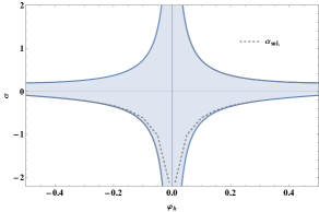
Thus, this regularity condition constrains the values of parameters (α,λ𝛼𝜆\alpha,\lambda) and the scalar field value near the horizon (φhsubscript𝜑\varphi_{h}). In Figure 1, we present the phase space for these parameters at a fixed value of λ𝜆\lambda. The shaded regions enclosed by the solid lines represent valid parameters for hairy black hole solutions. Points lying on the solid lines themselves are not considered valid.
Refer to caption
Figure 1: Phase space of α𝛼\alpha and φhsubscript𝜑\varphi_{h} for λ=0.1𝜆0.1\lambda=0.1 in the symmetric phase
Refer to caption
(a) Metric solutions with α=0.8𝛼0.8\alpha=-0.8
Refer to caption
(b) Metric solutions with α=3.5𝛼3.5\alpha=3.5
Refer to caption
(c) Scalar field solutions
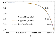
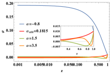
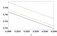
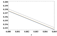
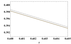
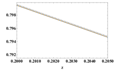
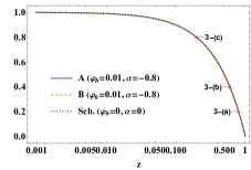
Figure 2: Hairy black hole solutions with φh=0.01subscript𝜑0.01\varphi_{h}=0.01 for various values of α𝛼\alpha. The black dotted line denotes the solutions of Schwarzschild black hole. The small regimes with the callout index (a)similar-to\sim(f) are plotted in Figure 3.
Refer to caption
(a) Case of α=0.8𝛼0.8\alpha=-0.8
Refer to caption
(b) Case of α=0.8𝛼0.8\alpha=-0.8
Refer to caption
(c) Case of α=0.8𝛼0.8\alpha=-0.8
Refer to caption
(d) Case of α=3.5𝛼3.5\alpha=3.5
Refer to caption
(e) Case of α=3.5𝛼3.5\alpha=3.5
Refer to caption
(f) Case of α=3.5𝛼3.5\alpha=3.5
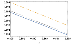
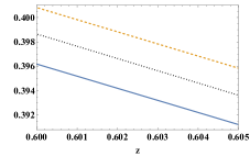
Figure 3: The comparison of metric solutions for hairy black holes and the Schwarzschild black hole. When α=0.8𝛼0.8\alpha=-0.8, hairy black holes exhibit a slight departure from the Schwarzschild black holes which shows the isotropic property (A/B=1𝐴𝐵1A/B=1) through the radial distance of z𝑧z. This deviation, though subtle, leads to noticeably distinct behavior in their QNMs. Conversely, for α=3.5𝛼3.5\alpha=3.5, the hairy black hole solutions show a much weaker deviations from the Schwarzschild metric across the radial distance.

To obtain the solutions, we impose the boundary value of φhsubscript𝜑\varphi_{h} for given values of α𝛼\alpha and λ𝜆\lambda and numerically solve the equations of motion (5.1)-(5.7) from the near horizon (z=zhϵ𝑧subscript𝑧italic-ϵz=z_{h}-\epsilon) to infinity (z=ϵ𝑧italic-ϵz=\epsilon). Here, Ahsubscript𝐴A_{h} is determined by the boundary conditions at infinity. To perform numerical calculation, we fixed zh=1subscript𝑧1z_{h}=1 and ϵ=1050italic-ϵsuperscript1050\epsilon=10^{-50} and used “NDSolve" implemented in Mathematica with precision up to 300300300. High precision and accuracy in constructing the background solution are crucial for reliable computation of quasinormal frequencies. This is because numerical errors in the background solution directly propagate to the calculated frequencies. As mentioned in [26], numerical solutions were not found in the entire valid parameter space but found beyond the certain value of α𝛼\alpha, which is denoted as αsol.subscript𝛼sol.\alpha_{\textrm{sol.}} in Figure 1. The absence of solutions in the region α<αsol.𝛼subscript𝛼sol.\alpha<\alpha_{\textrm{sol.}} is discussed in [26]. We present the numerically generated hairy black hole solutions in the symmetric phase for two different scalar field values at the horizon (φhsubscript𝜑\varphi_{h}). Given the value of λ=0.1𝜆0.1\lambda=0.1, Figure 3 shows the numerical solutions for the metric and scalar field with φh=0.01subscript𝜑0.01\varphi_{h}=0.01, comparing with the Schwarzschil black holes. To highlight the contrasting behavior of the solutions, Figure 3 zooms in on a smaller region of the z𝑧z-axis. This magnified view clearly reveals a significantly more pronounced anisotropy (A/B1𝐴𝐵1A/B\neq 1) in the metric for large negative α𝛼\alpha values compared to positive α𝛼\alpha values.

5.2  Scalar Field Perturbation

We consider a linearized perturbation of the complex scalar field around the background solution

φ(z)φ(z)+δφ(v,z,θ,ϕ),similar-to𝜑𝑧𝜑𝑧𝛿𝜑𝑣𝑧𝜃italic-ϕ\displaystyle\varphi(z)\sim\varphi(z)+\delta\varphi(v,z,\theta,\phi), (5.16)

so the linearized equation becomes

(αα+fφφ𝒢)δφ(z)+fφφ𝒢δφ(z)=0.subscript𝛼superscript𝛼subscript𝑓superscript𝜑𝜑𝒢𝛿𝜑𝑧subscript𝑓superscript𝜑𝜑𝒢𝛿superscript𝜑𝑧0\displaystyle\bigg{(}\nabla_{\alpha}\nabla^{\alpha}+f_{\varphi^{*}\varphi}\,\mathcal{G}\bigg{)}\delta\varphi(z)+f_{\varphi^{*}\varphi}\,\mathcal{G}\delta\varphi^{*}(z)=0. (5.17)

Employing the following ansatz for scalar field perturbation

δφ(v,z,θ,ϕ)=l,mΦ(z)Ylm(θ,ϕ)eiωv,𝛿𝜑𝑣𝑧𝜃italic-ϕsubscript𝑙𝑚Φ𝑧subscript𝑌𝑙𝑚𝜃italic-ϕsuperscript𝑒𝑖𝜔𝑣\displaystyle\delta\varphi(v,z,\theta,\phi)=\sum_{l,m}\Phi(z)Y_{lm}(\theta,\phi)e^{-i\omega v}, (5.18)

and using

1Y1sinθθ(sinθYθ)+1Y1sin2θ2Yϕ2=l(l+1)=γ,1𝑌1𝜃𝜃𝜃𝑌𝜃1𝑌1superscript2𝜃superscript2𝑌superscriptitalic-ϕ2𝑙𝑙1𝛾\displaystyle\frac{1}{Y}\frac{1}{\sin\theta}\frac{\partial}{\partial\theta}\bigg{(}\sin\theta\frac{\partial Y}{\partial\theta}\bigg{)}+\frac{1}{Y}\frac{1}{\sin^{2}\theta}\frac{\partial^{2}Y}{\partial\phi^{2}}=-l(l+1)=-\gamma, (5.19)

the linearized scalar field equation (5.17) is written as

z2A(z)B(z)Φ′′(z)+12(z2B(z)A(z)+z2A(z)B(z)+4iωB(z)A(z)B(z))Φ(z)superscript𝑧2𝐴𝑧𝐵𝑧superscriptΦ′′𝑧12superscript𝑧2𝐵𝑧superscript𝐴𝑧superscript𝑧2𝐴𝑧superscript𝐵𝑧4𝑖𝜔𝐵𝑧𝐴𝑧𝐵𝑧superscriptΦ𝑧\displaystyle z^{2}A(z)B(z)\Phi^{\prime\prime}(z)+\frac{1}{2}\bigg{(}z^{2}B(z)A^{\prime}(z)+z^{2}A(z)B^{\prime}(z)+4i\omega B(z)\sqrt{\frac{A(z)}{B(z)}}\bigg{)}\Phi^{\prime}(z)
+1z2(A(z)(𝒢f~φφ(φ)γz2)2iωzB(z)A(z)B(z))Φ(z)=01superscript𝑧2𝐴𝑧𝒢subscript~𝑓superscript𝜑𝜑𝜑𝛾superscript𝑧22𝑖𝜔𝑧𝐵𝑧𝐴𝑧𝐵𝑧Φ𝑧0\displaystyle+\frac{1}{z^{2}}\bigg{(}A(z)\left(\mathcal{G}\tilde{f}_{\varphi^{*}\varphi}(\varphi)-\gamma z^{2}\right)-2i\omega zB(z)\sqrt{\frac{A(z)}{B(z)}}\bigg{)}\Phi(z)=0 (5.20)

and

f~φφ=α6λφ12.subscript~𝑓superscript𝜑𝜑𝛼6𝜆superscriptsubscript𝜑12\displaystyle\tilde{f}_{\varphi^{*}\varphi}=\alpha-6\lambda\varphi_{1}^{2}. (5.21)

Let us investigate the asymptotic solution of (5.20) at both boundaries. Near the horizon, the perturbation equation is expanded as

z3(zzh)Φ′′(z)+[z32iωzAhBh]Φ(z)superscript𝑧3𝑧subscript𝑧superscriptΦ′′𝑧delimited-[]superscript𝑧32𝑖𝜔𝑧subscript𝐴subscript𝐵superscriptΦ𝑧\displaystyle z^{3}\left(z-z_{h}\right)\Phi^{\prime\prime}(z)+\left[z^{3}-\frac{2i\omega z}{\sqrt{A_{h}B_{h}}}\right]\Phi^{\prime}(z)
+[γBhz4z4(Bh(3z2zh)+2)(f′′(φh)+φh,1(zhz)f(3)(φh))+2iωAhBh]Φ(z)=0,delimited-[]𝛾subscript𝐵𝑧4superscript𝑧4subscript𝐵3𝑧2subscript𝑧2superscript𝑓′′subscript𝜑subscript𝜑1subscript𝑧𝑧superscript𝑓3subscript𝜑2𝑖𝜔subscript𝐴subscript𝐵Φ𝑧0\displaystyle+\bigg{[}\frac{\gamma}{B_{h}}z-4z^{4}\left(B_{h}\left(3z-2z_{h}\right)+2\right)(f^{\prime\prime}\left(\varphi_{h}\right)+\varphi_{h,1}\left(z_{h}-z\right)f^{(3)}\left(\varphi_{h}\right))+\frac{2i\omega}{\sqrt{A_{h}B_{h}}}\bigg{]}\Phi(z)=0, (5.22)

and plugging Φ(z)(zhz)p=ϵpsimilar-toΦ𝑧superscriptsubscript𝑧𝑧𝑝superscriptitalic-ϵ𝑝\Phi(z)\sim(z_{h}-z)^{p}=\epsilon^{p} into above it expands

ϵp[pϵ(pzh2+2iωAhBh)+1zh2iωAhBh4zh3(Bhzh+2)f′′(φh)+γBh+2p2zh]0.similar-tosuperscriptitalic-ϵ𝑝delimited-[]𝑝italic-ϵ𝑝superscriptsubscript𝑧22𝑖𝜔subscript𝐴subscript𝐵1subscript𝑧2𝑖𝜔subscript𝐴subscript𝐵4superscriptsubscript𝑧3subscript𝐵subscript𝑧2superscript𝑓′′subscript𝜑𝛾subscript𝐵2superscript𝑝2subscript𝑧0\displaystyle\epsilon^{p}\left[\frac{p}{\epsilon}\left(-pz_{h}^{2}+\frac{2i\omega}{\sqrt{A_{h}B_{h}}}\right)+\frac{1}{z_{h}}\frac{2i\omega}{\sqrt{A_{h}B_{h}}}-4z_{h}^{3}\left(B_{h}z_{h}+2\right)f^{\prime\prime}\left(\varphi_{h}\right)+\frac{\gamma}{B_{h}}+2p^{2}z_{h}\right]\sim 0. (5.23)

For the equation not to be singular, the first term should vanish. This requires p𝑝p to take values:

p=0orp=1zh22iωAhBhformulae-sequence𝑝0or𝑝1superscriptsubscript𝑧22𝑖𝜔subscript𝐴subscript𝐵\displaystyle p=0\qquad\textrm{or}\qquad p=\frac{1}{z_{h}^{2}}\frac{2i\omega}{\sqrt{A_{h}B_{h}}} (5.24)

which yield

δφ(v,z)=eiωvconst.𝛿𝜑𝑣𝑧superscript𝑒𝑖𝜔𝑣const.\displaystyle\delta\varphi(v,z)=e^{-i\omega v}\textrm{const.} (5.25)
or δφ(v,z)=eiωv(zhz)2iωzh2AhBh=eiω(v2zh2AhBhlog(zhz)).𝛿𝜑𝑣𝑧superscript𝑒𝑖𝜔𝑣superscriptsubscript𝑧𝑧2𝑖𝜔superscriptsubscript𝑧2subscript𝐴subscript𝐵superscript𝑒𝑖𝜔𝑣2superscriptsubscript𝑧2subscript𝐴subscript𝐵subscript𝑧𝑧\displaystyle\delta\varphi(v,z)=e^{-i\omega v}(z_{h}-z)^{\frac{2i\omega}{z_{h}^{2}\sqrt{A_{h}B_{h}}}}=e^{-i\omega\big{(}v-\frac{2}{z_{h}^{2}\sqrt{A_{h}B_{h}}}\log(z_{h}-z)\big{)}}. (5.26)

The first solution corresponds to the incoming mode. The second one is written as

δφ(v,z)=eiω(v2z+2c)=eiω(u+2c),𝛿𝜑𝑣𝑧superscript𝑒𝑖𝜔𝑣2subscript𝑧2𝑐superscript𝑒𝑖𝜔𝑢2𝑐\displaystyle\delta\varphi(v,z)=e^{-i\omega(v-2z_{*}+2c)}=e^{-i\omega(u+2c)}, (5.27)

where the outgoing null vector u=tz𝑢𝑡subscript𝑧u=t-z_{*} is used and zsubscript𝑧z_{*} is expanded near the horizon such as

z1zh2AhBh(1+iπlog(zh)+log(zhz))=1zh2AhBhlog(zhz)+c,similar-to-or-equalssubscript𝑧1superscriptsubscript𝑧2subscript𝐴subscript𝐵1𝑖𝜋subscript𝑧subscript𝑧𝑧1superscriptsubscript𝑧2subscript𝐴subscript𝐵subscript𝑧𝑧𝑐\displaystyle z_{*}\simeq\frac{1}{z_{h}^{2}\sqrt{A_{h}B_{h}}}(1+i\pi-\log(z_{h})+\log(z_{h}-z))=\frac{1}{z_{h}^{2}\sqrt{A_{h}B_{h}}}\log(z_{h}-z)+c, (5.28)

where c𝑐c indicates the first three terms in the second equality. This indicates that the second solution in (5.24) corresponds to the outgoing mode. Also, as shown in (5.26), the phase of this outgoing solution diverges and oscillates very fast when z𝑧z approaches zhsubscript𝑧z_{h} in (v,z)𝑣𝑧(v,z)-coordinate. Due to the limitations of numerical calculations on a grid, the rapid oscillations of the outgoing modes are not captured. Consequently, we can only impose the incoming boundary condition at the horizon, effectively excluding the outgoing modes from the numerical calculation.

Near infinity the perturbation equation (5.20) is expanded

Φ′′(z)+2iωz2Φ(z)2iωz3Φ(z)0,similar-to-or-equalssuperscriptΦ′′𝑧2𝑖𝜔superscript𝑧2superscriptΦ𝑧2𝑖𝜔superscript𝑧3Φ𝑧0\displaystyle\Phi^{\prime\prime}(z)+\frac{2i\omega}{z^{2}}\Phi^{\prime}(z)-\frac{2i\omega}{z^{3}}\Phi(z)\simeq 0, (5.29)

and the solution takes the following form

Φ(z)=c1ze2iωzic22ωz.Φ𝑧subscript𝑐1𝑧superscript𝑒2𝑖𝜔𝑧𝑖subscript𝑐22𝜔𝑧\displaystyle\Phi(z)=c_{1}ze^{\frac{2i\omega}{z}}-\frac{ic_{2}}{2\omega}z. (5.30)

To rigorously check this solution, we generalize the form to be

Φ(z)=c1zpe2iωzic22ωzp.Φ𝑧subscript𝑐1superscript𝑧𝑝superscript𝑒2𝑖𝜔𝑧𝑖subscript𝑐22𝜔superscript𝑧𝑝\displaystyle\Phi(z)=c_{1}z^{p}e^{\frac{2i\omega}{z}}-\frac{ic_{2}}{2\omega}z^{p}. (5.31)

and expand (5.29) near z0similar-to𝑧0z\sim 0. Then we obtain

zp3e2iωzA1z+1[A1(p2z24ipωz+2iω(z+2iω))+p2zp(z+2iω)+2iωγz]c1superscript𝑧𝑝3superscript𝑒2𝑖𝜔𝑧subscript𝐴1𝑧1delimited-[]subscript𝐴1superscript𝑝2superscript𝑧24𝑖𝑝𝜔𝑧2𝑖𝜔𝑧2𝑖𝜔superscript𝑝2𝑧𝑝𝑧2𝑖𝜔2𝑖𝜔𝛾𝑧subscript𝑐1\displaystyle\frac{z^{p-3}e^{\frac{2i\omega}{z}}}{A_{1}z+1}\bigg{[}A_{1}\left(p^{2}z^{2}-4ip\omega z+2i\omega(z+2i\omega)\right)+p^{2}z-p(z+2i\omega)+2i\omega-\gamma z\bigg{]}c_{1}
i2ωzp3A1z+1[A1p2z2+p2z+2ipωpz2iωγz]c20.similar-to-or-equals𝑖2𝜔superscript𝑧𝑝3subscript𝐴1𝑧1delimited-[]subscript𝐴1superscript𝑝2superscript𝑧2superscript𝑝2𝑧2𝑖𝑝𝜔𝑝𝑧2𝑖𝜔𝛾𝑧subscript𝑐20\displaystyle-\frac{i}{2\omega}\frac{z^{p-3}}{A_{1}z+1}\bigg{[}A_{1}p^{2}z^{2}+p^{2}z+2ip\omega-pz-2i\omega-\gamma z\bigg{]}c_{2}\simeq 0. (5.32)

Taking z0𝑧0z\rightarrow 0 limit, the first and second line require p=1+2iA1ω𝑝12𝑖subscript𝐴1𝜔p=1+2iA_{1}\omega and p=1𝑝1p=1 respectively and they yield

δφ(v,z)c1eiωve2iωz(z1+2iA1ω+)+c2eiωv(z+).similar-to𝛿𝜑𝑣𝑧subscript𝑐1superscript𝑒𝑖𝜔𝑣superscript𝑒2𝑖𝜔𝑧superscript𝑧12𝑖subscript𝐴1𝜔subscript𝑐2superscript𝑒𝑖𝜔𝑣𝑧\displaystyle\delta\varphi(v,z)\sim c_{1}e^{-i\omega v}e^{\frac{2i\omega}{z}}(z^{1+2iA_{1}\omega}+\cdots)+c_{2}e^{-i\omega v}(z+\cdots). (5.33)

The second term having c2subscript𝑐2c_{2} describes the incoming mode and is normalisable. The first term having c1subscript𝑐1c_{1} is rewritten as

δφ(v,z)=eiω(v2z2A1logz)+=eiω(v2z)+=eiωu+,𝛿𝜑𝑣𝑧superscript𝑒𝑖𝜔𝑣2𝑧2subscript𝐴1𝑧superscript𝑒𝑖𝜔𝑣2subscript𝑧superscript𝑒𝑖𝜔𝑢\displaystyle\delta\varphi(v,z)=e^{-i\omega(v-\frac{2}{z}-2A_{1}\log z)}+\cdots=e^{-i\omega(v-2z_{*})}+\cdots=e^{-i\omega u}+\cdots, (5.34)

where u=tz𝑢𝑡subscript𝑧u=t-z_{*} is an outgoing null vector and zsubscript𝑧z_{*} in (5.2) is expanded in z0𝑧0z\rightarrow 0 limit

z=1z21ABdz1z+A1logz.subscript𝑧1superscript𝑧21𝐴𝐵differential-d𝑧similar-to-or-equals1𝑧subscript𝐴1𝑧\displaystyle z_{*}=-\int\frac{1}{z^{2}}\frac{1}{\sqrt{AB}}{\rm d}z\simeq\frac{1}{z}+A_{1}\log z. (5.35)

This indicates that the first term describes the outgoing mode but is non-normalizable and oscillates more rapidly as z𝑧z approaches 00 in (v,z)𝑣𝑧(v,z)-coordinate. Here, we want to impose the outgoing boundary condition. This situation is problematic. To resolve this we redefine Φ(z)Φ𝑧\Phi(z) as

Φ(z)e2iωzz2iA1ωΦ~(z)similar-toΦ𝑧superscript𝑒2𝑖𝜔𝑧superscript𝑧2𝑖subscript𝐴1𝜔~Φ𝑧\displaystyle\Phi(z)\sim e^{\frac{2i\omega}{z}}z^{2iA_{1}\omega}\tilde{\Phi}(z) (5.36)

and the new field Φ~(z)~Φ𝑧\tilde{\Phi}(z) becomes

Φ~(z)=c1zic22ωe2iωzz12iA1ω.~Φ𝑧subscript𝑐1𝑧𝑖subscript𝑐22𝜔superscript𝑒2𝑖𝜔𝑧superscript𝑧12𝑖subscript𝐴1𝜔\displaystyle\tilde{\Phi}(z)=c_{1}z-\frac{ic_{2}}{2\omega}e^{-\frac{2i\omega}{z}}z^{1-2iA_{1}\omega}. (5.37)

Then, the incoming mode becomes non-normalizable and is not captured by the numerical calculation due to the fast oscillation, while the outgoing mode becomes normalizable and behaves smoothly. Rewriting the perturbation equation (5.20) in terms of Φ~(z)~Φ𝑧\tilde{\Phi}(z), it yields

Φ~′′(z)+[2iωz2(1A(z)B(z)+2(A1z1))+12(A(z)A(z)+B(z)B(z))]Φ~(z)superscript~Φ′′𝑧delimited-[]2𝑖𝜔superscript𝑧21𝐴𝑧𝐵𝑧2subscript𝐴1𝑧112superscript𝐴𝑧𝐴𝑧superscript𝐵𝑧𝐵𝑧superscript~Φ𝑧\displaystyle\tilde{\Phi}^{\prime\prime}(z)+\bigg{[}\frac{2i\omega}{z^{2}}\left(\frac{1}{\sqrt{A(z)B(z)}}+2(A_{1}z-1)\right)+\frac{1}{2}\left(\frac{A^{\prime}(z)}{A(z)}+\frac{B^{\prime}(z)}{B(z)}\right)\bigg{]}\tilde{\Phi}^{\prime}(z)
+[RGBf~φφγz2z4B(z)4ω2(A1z1)z4(1A(z)B(z)+(A1z1))\displaystyle+\bigg{[}\frac{R_{\text{GB}}\tilde{f}_{\varphi^{*}\varphi}-\gamma z^{2}}{z^{4}B(z)}-\frac{4\omega^{2}\left(A_{1}z-1\right)}{z^{4}}\left(\frac{1}{\sqrt{A(z)B(z)}}+\left(A_{1}z-1\right)\right)
iωz3(2A1z4z(A1z1)(A(z)A(r)+B(z)B(r))+2A(z)B(z))]Φ~(z)=0.\displaystyle-\frac{i\omega}{z^{3}}\left(2A_{1}z-4-z\left(A_{1}z-1\right)\left(\frac{A^{\prime}(z)}{A(r)}+\frac{B^{\prime}(z)}{B(r)}\right)+\frac{2}{\sqrt{A(z)B(z)}}\right)\bigg{]}\tilde{\Phi}(z)=0. (5.38)

By adopting the numerical method explained in Section 3.4, we will numerically calculate the quasinormal frequency ω𝜔\omega in (5.38) and display their values in the following subsection.

5.3  Our Numerical Results

We first consider the Schwarzschild black hole, which is the solution with φ=0𝜑0\varphi=0, and examine its stability according to the value of α𝛼\alpha. By computing the quasinormal frequency, we found that a positive imaginary part of the frequency, Im[ω]delimited-[]𝜔[\omega], emerges at a critical value, αSch.0.1815subscript𝛼Sch.0.1815\alpha_{\textrm{Sch.}}\approx 0.1815 as shown in Figure 4. This indicates that the corresponding system becomes unstable ααSch.𝛼subscript𝛼Sch.\alpha\geq\alpha_{\textrm{Sch.}}. Here, we want to argue that this instability triggers a transition from the Schwarzschild black hole to a hairy black hole, and the hairy black hole will be formed not in the symmetric phase but in the symmetry-broken phase. To support this argument, we show that the hairy black holes with ααSch.𝛼subscript𝛼Sch.\alpha\geq\alpha_{\textrm{Sch.}} are unstable in the symmetric phase but stable in the symmetry-broken phase. This section focuses solely on the quasinormal frequencies of hairy black holes in the symmetric phase for various α𝛼\alpha values. The stability analysis of hairy black holes in the symmetry-broken phase will be addressed in Section 6.
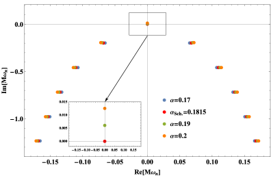
Refer to caption
Re[Mωn𝑀subscript𝜔𝑛M\omega_{n}] Im[Mωn𝑀subscript𝜔𝑛M\omega_{n}]
α𝛼\alpha=0.17 ±plus-or-minus\pm 0.06528 -0.19795
±plus-or-minus\pm 0.10718 -0.45845
±plus-or-minus\pm 0.13196 -0.71851
±plus-or-minus\pm 0.15043 0.97682
αSch.subscript𝛼Sch.absent\alpha_{\textrm{Sch.}}\approx 0.1815 0 0.00002
±plus-or-minus\pm 0.06826 -0.19618
±plus-or-minus\pm 0.11012 -0.45776
±plus-or-minus\pm 0.13483 -0.71820
±plus-or-minus\pm 0.15324 -0.97669
α𝛼\alpha=0.19 0 0.00600
±plus-or-minus\pm 0.07013 -0.19489
±plus-or-minus\pm 0.11208 -0.45728
±plus-or-minus\pm 0.13677 -0.71798
±plus-or-minus\pm 0.15513 -0.97662
α𝛼\alpha=0.20 0 0.01254
±plus-or-minus\pm 0.07198 -0.19340
±plus-or-minus\pm 0.11415 -0.45675
±plus-or-minus\pm 0.13881 -0.71775
±plus-or-minus\pm 0.15712 -0.97654
\captionlistentry

[table]Sch

Figure 4: QNMs of Schwarzschild black holes for serval values α𝛼\alpha

To compute the eigenvalues, we performed calculations with grids of size 100 and 140, resulting in 100 and 140 eigenvalues, respectively. We then identified eigenvalues where both calculations agreed within a tolerance of 102superscript10210^{-2} for both the real and imaginary parts. Finally, we plotted the corresponding eigenfunctions associated with these converged eigenvalues to verify that they satisfy the boundary conditions. Figure 5 shows the quasinormal frequencies for α=0.2,0.8,0.9,1,1.1,1.2,1.3𝛼0.20.80.911.11.21.3\alpha=-0.2,-0.8,-0.9,-1,-1.1,-1.2,-1.3 and 1.41.4-1.4, generated on the background solution with φh=0.01subscript𝜑0.01\varphi_{h}=0.01 for a fixed value of λ=0.1𝜆0.1\lambda=0.1. Figure 6 demonstrates the quasinormal frequencies for α=0.12,0.1815,0.6,1,1.6,2.1,2.4𝛼0.120.18150.611.62.12.4\alpha=0.12,0.1815,0.6,1,1.6,2.1,2.4 and 2.82.82.8 on the same background. The detailed numerical values for the QNMs presented in Figure 5 and 6 can be found in Appendix A.

Our results show that the imaginary parts of the QNM frequencies are all negative for the negative values of α𝛼\alpha. In Figure 5, the QNMs exhibit a well arranged line of spectrum at α=0.2𝛼0.2\alpha=-0.2. As α𝛼\alpha decreases towards more negative values, a progressive shift is observed in the higher-order QNMs. The fifth QNM exhibits this behavior first, moving inwards and upwards relative to the main QNMs’ array. Subsequently, at larger negative α𝛼\alpha values, the sixth QNM starts displaying the same behavior. This sequence of inward and upward shifts with increasing negative α𝛼\alpha forms the additional array of the QNM spectrum inside the outer array of the QNMs. However, pushing α𝛼\alpha to even more negative values leads to a depletion of higher-frequency QNMs, resulting in a sparser spectrum at α=1.4𝛼1.4\alpha=-1.4. Figure 3 reveals that the metric exhibits increasing anisotropy (A/B1𝐴𝐵1A/B\neq 1) with more negative values of α𝛼\alpha. This deviation from isotropy (A/B=1𝐴𝐵1A/B=1) is suspected to be a contributing factor to the emergence of the exotic (cases of α=0.8𝛼0.8\alpha=-0.8 to 1.21.2-1.2) and diminishing (cases of α=1.3𝛼1.3\alpha=-1.3 and 1.41.4-1.4) QNM spectrum observed at large negative α𝛼\alpha values.

For the positive values of α𝛼\alpha, we found that the imaginary parts of the QNM frequencies become positive at α=0.1815𝛼0.1815\alpha=0.1815 (denoted as αcrit.subscript𝛼crit.\alpha_{\textrm{crit.}}). This positive imaginary part indicates that the hairy black hole becomes dynamically unstable in the regime ααcrit.𝛼subscript𝛼crit.\alpha\geq\alpha_{\textrm{crit.}}. We demonstrated the corresponding eigenfunctions to ensure these eigenvalues and examined their behaviors in Figure 14 in Appendix B. To investigate the angular dependence of the QNM spectrum in this case, we further checked the QNM behavior for different values of l𝑙l. The results are presented in Figure 15 in Appendix C. Figure 6 illustrates that as the value of α𝛼\alpha increases, lower-frequency QNMs (with smaller imaginary parts) transition to having positive imaginary parts. As the value of α𝛼\alpha increases further, higher-frequency QNMs (with larger imaginary parts) progressively disappear from the spectrum. For α=3.5𝛼3.5\alpha=3.5, the QNMs exhibit purely positive imaginary frequencies. This implies that the oscillations of the perturbed scalar fields vanish and are only damped or growing at this value. We also computed the QNMs frequencies for α=0.3,0.184,0.1848𝛼0.30.1840.1848\alpha=-0.3,0.184,0.1848 and 0.40.40.4 for φh=0.1subscript𝜑0.1\varphi_{h}=0.1 and λ=0.1𝜆0.1\lambda=0.1 and plotted them in Figure 7. Table 2 presents the numerically computed QNM frequencies. Black colored numbers indicate a high degree of accuracy, with a numerical error less than 105superscript10510^{-5} between the results obtained from grids of size 100100100 and 140140140. Conversely, gray colored numbers signify potential numerical inaccuracy in those digits. In this case, we found that the critical value of α𝛼\alpha appears at αcrit.=0.1848subscript𝛼crit.0.1848\alpha_{\textrm{crit.}}=0.1848. Since these critical values of α𝛼\alpha are involved in dynamical stability, their values differ from those computed in [26], which are sufficient conditions.
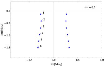
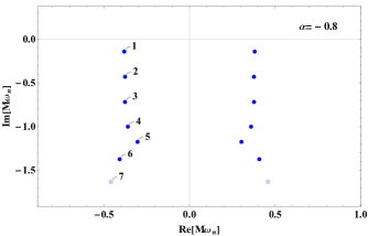
Refer to caption

     Refer to caption

Refer to caption

     Refer to caption

Refer to caption

     Refer to caption

Refer to caption

     Refer to caption

Figure 5: QNMs with negative values of α𝛼\alpha for φh=0.01subscript𝜑0.01\varphi_{h}=0.01. Blue dots are tolerable less than 103superscript10310^{-3}, whereas lighter blue dots have a tolerance of 102superscript10210^{-2}.
Refer to caption

     Refer to caption

Refer to caption

     Refer to caption

Refer to caption

     Refer to caption

Refer to caption

     Refer to caption

Figure 6: QNMs with positive values of α𝛼\alpha for φh=0.01subscript𝜑0.01\varphi_{h}=0.01. Blue dots are tolerable less than 103superscript10310^{-3}, whereas lighter blue dots have a tolerance of 102superscript10210^{-2}.
Refer to caption
Re[Mωn𝑀subscript𝜔𝑛M\omega_{n}] Im[Mωn𝑀subscript𝜔𝑛M\omega_{n}]
1 ±0.25244plus-or-minus0.25244\pm 0.25244 0.132430.13243-0.13243
2 ±0.23104plus-or-minus0.23104\pm 0.23104 0.413270.41327-0.41327
3 ±0.22792plus-or-minus0.22792\pm 0.22792 0.697140.69714-0.69714
4 ±0.24934plus-or-minus0.24934\pm 0.24934 0.950780.95078-0.95078
5 ±0.28562plus-or-minus0.28562\pm 0.28562 1.194281.19428-1.19428
6 ±0.32339plus-or-minus0.32339\pm 0.32{\color[rgb]{.5,.5,.5}339} 1.440881.44088-1.44{\color[rgb]{.5,.5,.5}088}
Refer to caption
Re[Mωn𝑀subscript𝜔𝑛M\omega_{n}] Im[Mωn𝑀subscript𝜔𝑛M\omega_{n}]
1 ±0.06855plus-or-minus0.06855\pm 0.06855 0.195890.19589-0.19589
2 ±0.11334plus-or-minus0.11334\pm 0.11334 0.455810.45581-0.45581
3 ±0.14435plus-or-minus0.14435\pm 0.1443{\color[rgb]{.5,.5,.5}5} 0.713440.71344-0.7134{\color[rgb]{.5,.5,.5}4}
4 ±0.17341plus-or-minus0.17341\pm 0.1734{\color[rgb]{.5,.5,.5}1} 0.967710.96771-0.9677{\color[rgb]{.5,.5,.5}1}
5 ±0.20376plus-or-minus0.20376\pm 0.203{\color[rgb]{.5,.5,.5}76} 1.219341.21934-1.219{\color[rgb]{.5,.5,.5}34}
Refer to caption
Re[Mωn𝑀subscript𝜔𝑛M\omega_{n}] Im[Mωn𝑀subscript𝜔𝑛M\omega_{n}]
1 00 0.000150.000150.00015
2 ±0.06876plus-or-minus0.06876\pm 0.06876 0.195760.19576-0.19576
3 ±0.11359plus-or-minus0.11359\pm 0.11359 0.455730.45573-0.45573
4 ±0.14467plus-or-minus0.14467\pm 0.1446{\color[rgb]{.5,.5,.5}7} 0.713340.71334-0.7133{\color[rgb]{.5,.5,.5}4}
5 ±0.17385plus-or-minus0.17385\pm 0.173{\color[rgb]{.5,.5,.5}85} 0.967570.96757-0.967{\color[rgb]{.5,.5,.5}57}
6 ±0.20436plus-or-minus0.20436\pm 0.204{\color[rgb]{.5,.5,.5}36} 1.219141.21914-1.219{\color[rgb]{.5,.5,.5}14}
Refer to caption
Re[Mωn𝑀subscript𝜔𝑛M\omega_{n}] Im[Mωn𝑀subscript𝜔𝑛M\omega_{n}]
1 00 0.102370.102370.10237
2 ±0.07985plus-or-minus0.07985\pm 0.07985 0.159110.15911-0.15911
3 ±0.14962plus-or-minus0.14962\pm 0.14962 0.423910.42391-0.42391
4 ±0.22154plus-or-minus0.22154\pm 0.22154 0.656860.65686-0.65686
5 ±0.29939plus-or-minus0.29939\pm 0.29939 0.889370.88937-0.88937
6 ±0.37565plus-or-minus0.37565\pm 0.37565 1.121841.12184-1.12184
7 ±0.45030plus-or-minus0.45030\pm 0.450{\color[rgb]{.5,.5,.5}30} 1.352391.35239-1.352{\color[rgb]{.5,.5,.5}39}
\captionlistentry

[table]A table beside a figure

Figure 7: QNMs with various values of α𝛼\alpha for φh=0.1subscript𝜑0.1\varphi_{h}=0.1. Blue dots are tolerable less than 103superscript10310^{-3}, whereas lighter blue dots have a tolerance of 102superscript10210^{-2}.

6.  Quasinormal Modes for Hairy Black Holes in the Symmetry-Broken Phase

This section demonstrates the numerically generated hairy black holes’ solution in the symmetry-broken phase and shows their QNMs.

6.1  Background solution

When α𝛼\alpha is positive, the interaction potential V𝑉V forms degenerate vacuums, and the stable minima are described by

φ=vvaceiβ,vvac=α2λ,formulae-sequencedelimited-⟨⟩𝜑subscript𝑣vacsuperscript𝑒𝑖𝛽subscript𝑣vac𝛼2𝜆\displaystyle\langle\varphi\rangle=v_{\textrm{vac}}\,e^{i\beta},\qquad v_{\textrm{vac}}=\sqrt{\frac{\alpha}{2\,\lambda}}, (6.1)

where the vacuum states are labeled by the parameter β𝛽\beta. These ground states do not respect the symmetry of the Lagrangian, which indicates that symmetry is spontaneously broken in the vacuum. We expand a field around a ground state v𝑣v by reparameterizing it as follows

φ(z)=(vvac+σ(z)2)eiθ(z).𝜑𝑧subscript𝑣vac𝜎𝑧2superscript𝑒𝑖𝜃𝑧\displaystyle\varphi(z)=\bigg{(}v_{\textrm{vac}}+\frac{\sigma(z)}{\sqrt{2}}\bigg{)}e^{i\theta(z)}. (6.2)

Here, the new variables σ(z)𝜎𝑧\sigma(z) and θ(z)𝜃𝑧\theta(z) are physical fields because they are excitations above the vacuum. Then we rewrite the Lagrangian in terms of σ(z)𝜎𝑧\sigma(z) and θ(z)𝜃𝑧\theta(z)

φ=12ασ(z)ασ(z)(vvac+σ(z)2)2αθ(z)αθ(z)+f(σ)𝒢subscript𝜑12subscript𝛼𝜎𝑧superscript𝛼𝜎𝑧superscriptsubscript𝑣vac𝜎𝑧22subscript𝛼𝜃𝑧superscript𝛼𝜃𝑧𝑓𝜎𝒢\displaystyle\mathcal{L}_{\varphi}=-\frac{1}{2}\nabla_{\alpha}\sigma(z)\nabla^{\alpha}\sigma(z)-\bigg{(}v_{\textrm{vac}}+\frac{\sigma(z)}{\sqrt{2}}\bigg{)}^{2}\nabla_{\alpha}\theta(z)\nabla^{\alpha}\theta(z)+f(\sigma)\,\mathcal{G} (6.3)

where

f(σ)=ασ(z)2αλσ(z)3λ4σ(z)4.𝑓𝜎𝛼𝜎superscript𝑧2𝛼𝜆𝜎superscript𝑧3𝜆4𝜎superscript𝑧4\displaystyle f(\sigma)=-\alpha\,\sigma(z)^{2}-\sqrt{\alpha\,\lambda}\;\sigma(z)^{3}-\frac{\lambda}{4}\,\sigma(z)^{4}. (6.4)

Einstein equations and scalar field equations read

1κ2(Rμν12Rgμν)=[12γσγσ(vvac+σ2)2γθγθ]gμν1superscript𝜅2subscript𝑅𝜇𝜈12𝑅subscript𝑔𝜇𝜈delimited-[]12subscript𝛾𝜎superscript𝛾𝜎superscriptsubscript𝑣vac𝜎22subscript𝛾𝜃superscript𝛾𝜃subscript𝑔𝜇𝜈\displaystyle\frac{1}{\kappa^{2}}\bigg{(}R_{\mu\nu}-\frac{1}{2}Rg_{\mu\nu}\bigg{)}=\bigg{[}-\frac{1}{2}\nabla_{\gamma}\sigma\nabla^{\gamma}\sigma-\bigg{(}v_{\textrm{vac}}+\frac{\sigma}{\sqrt{2}}\bigg{)}^{2}\nabla_{\gamma}\theta\nabla^{\gamma}\theta\bigg{]}g_{\mu\nu}
+μσνσ+2(vvac+σ2)2μθνθ(gρμgλν+gλμgρν)ηκλαβR~ργγαβκf(σ),\displaystyle\qquad\qquad+\nabla_{\mu}\sigma\nabla_{\nu}\sigma+2\bigg{(}v_{\textrm{vac}}+\frac{\sigma}{\sqrt{2}}\bigg{)}^{2}\nabla_{\mu}\theta\,\nabla_{\nu}\theta-(g_{\rho\mu}g_{\lambda\nu}+g_{\lambda\mu}g_{\rho\nu})\eta^{\kappa\lambda\alpha\beta}\tilde{R}^{\rho\gamma}{}_{\alpha\beta}\nabla_{\gamma}\nabla_{\kappa}f(\sigma), (6.5)
αασ2(vvac+σ2)αθαθ+fσ𝒢=0,(vvac+σ2)ααθ+2ασαθ=0.formulae-sequencesuperscript𝛼subscript𝛼𝜎2subscript𝑣vac𝜎2superscript𝛼𝜃subscript𝛼𝜃subscript𝑓𝜎𝒢0subscript𝑣vac𝜎2superscript𝛼subscript𝛼𝜃2superscript𝛼𝜎subscript𝛼𝜃0\displaystyle\nabla^{\alpha}\nabla_{\alpha}\sigma-\sqrt{2}\bigg{(}v_{\textrm{vac}}+\frac{\sigma}{\sqrt{2}}\bigg{)}\nabla^{\alpha}\theta\,\nabla_{\alpha}\theta+f_{\sigma}\,\mathcal{G}=0,\qquad\bigg{(}v_{\textrm{vac}}+\frac{\sigma}{\sqrt{2}}\bigg{)}\nabla^{\alpha}\nabla_{\alpha}\theta+\sqrt{2}\,\nabla^{\alpha}\sigma\nabla_{\alpha}\theta=0. (6.6)

Consequently, they take the following explicit form:

1z2(11BzBB)+κ2(v+σ2)2θ2+12κ2(σ)21superscript𝑧211𝐵𝑧superscript𝐵𝐵superscript𝜅2superscript𝑣𝜎22superscript𝜃212superscript𝜅2superscriptsuperscript𝜎2\displaystyle\frac{1}{z^{2}}\bigg{(}1-\frac{1}{B}-\frac{zB^{\prime}}{B}\bigg{)}+\kappa^{2}\left(v+\frac{\sigma}{\sqrt{2}}\right)^{2}\theta^{\prime 2}+\frac{1}{2}\kappa^{2}(\sigma^{\prime})^{2}
+4κ2[z2(13B)BσfσB2z(B1)(zfσσ(σ)2+fσ(zσ′′+2σ))]=0,4superscript𝜅2delimited-[]superscript𝑧213𝐵superscript𝐵superscript𝜎subscript𝑓𝜎𝐵2𝑧𝐵1𝑧subscript𝑓𝜎𝜎superscriptsuperscript𝜎2subscript𝑓𝜎𝑧superscript𝜎′′2superscript𝜎0\displaystyle\qquad+4\kappa^{2}\left[\frac{z^{2}(1-3B)B^{\prime}\sigma^{\prime}f_{\sigma}}{B}-2z(B-1)\bigg{(}zf_{\sigma\sigma}(\sigma^{\prime})^{2}+f_{\sigma}\left(z\sigma^{\prime\prime}+2\sigma^{\prime}\right)\bigg{)}\right]=0, (6.7)
1z(BBAA)2κ2(v+σ2)2θ2κ2(σ)21𝑧superscript𝐵𝐵superscript𝐴𝐴2superscript𝜅2superscript𝑣𝜎22superscript𝜃2superscript𝜅2superscriptsuperscript𝜎2\displaystyle\frac{1}{z}\bigg{(}\frac{B^{\prime}}{B}-\frac{A^{\prime}}{A}\bigg{)}-2\kappa^{2}\left(v+\frac{\sigma}{\sqrt{2}}\right)^{2}\theta^{\prime 2}-\kappa^{2}(\sigma^{\prime})^{2}
+κ2[4z2(3B1)(BBAA)σfσ+8z(B1)(zfσσ(σ)2+fσ(zσ′′+2σ))]=0,superscript𝜅2delimited-[]4superscript𝑧23𝐵1superscript𝐵𝐵superscript𝐴𝐴superscript𝜎subscript𝑓𝜎8𝑧𝐵1𝑧subscript𝑓𝜎𝜎superscriptsuperscript𝜎2subscript𝑓𝜎𝑧superscript𝜎′′2superscript𝜎0\displaystyle\qquad+\kappa^{2}\left[4z^{2}(3B-1)\left(\frac{B^{\prime}}{B}-\frac{A^{\prime}}{A}\right)\sigma^{\prime}f_{\sigma}+8z(B-1)\bigg{(}zf_{\sigma\sigma}(\sigma^{\prime})^{2}+f_{\sigma}\left(z\sigma^{\prime\prime}+2\sigma^{\prime}\right)\bigg{)}\right]=0, (6.8)
A′′2A+14z(zAA2)(BBAA)+κ2(v+σ2)2θ2+12κ2(σ)2superscript𝐴′′2𝐴14𝑧𝑧superscript𝐴𝐴2superscript𝐵𝐵superscript𝐴𝐴superscript𝜅2superscript𝑣𝜎22superscript𝜃212superscript𝜅2superscriptsuperscript𝜎2\displaystyle\frac{A^{\prime\prime}}{2A}+\frac{1}{4z}\left(\frac{zA^{\prime}}{A}-2\right)\left(\frac{B^{\prime}}{B}-\frac{A^{\prime}}{A}\right)+\kappa^{2}\left(v+\frac{\sigma}{\sqrt{2}}\right)^{2}\theta^{\prime 2}+\frac{1}{2}\kappa^{2}(\sigma^{\prime})^{2}
+2z2Bκ2[2zAA(σ2fσσ+σ′′fσ)+σfσ(zAA(3BBAA)+2(zA′′A+4AA))]=0,2superscript𝑧2𝐵superscript𝜅2delimited-[]2𝑧superscript𝐴𝐴superscript𝜎2subscript𝑓𝜎𝜎superscript𝜎′′subscript𝑓𝜎superscript𝜎subscript𝑓𝜎𝑧superscript𝐴𝐴3superscript𝐵𝐵superscript𝐴𝐴2𝑧superscript𝐴′′𝐴4superscript𝐴𝐴0\displaystyle\qquad+2z^{2}B\kappa^{2}\left[\frac{2zA^{\prime}}{A}\left(\sigma^{\prime 2}f_{\sigma\sigma}+\sigma^{\prime\prime}f_{\sigma}\right)+\sigma^{\prime}f_{\sigma}\left(\frac{zA^{\prime}}{A}\left(\frac{3B^{\prime}}{B}-\frac{A^{\prime}}{A}\right)+2\left(\frac{zA^{\prime\prime}}{A}+\frac{4A^{\prime}}{A}\right)\right)\right]=0, (6.9)

and

σ′′+(A2A+B2B)σ2(vvac+σ2)(θ)2superscript𝜎′′superscript𝐴2𝐴superscript𝐵2𝐵superscript𝜎2subscript𝑣vac𝜎2superscriptsuperscript𝜃2\displaystyle\sigma^{\prime\prime}+\bigg{(}\frac{A^{\prime}}{2A}+\frac{B^{\prime}}{2B}\bigg{)}\sigma^{\prime}-\sqrt{2}\bigg{(}v_{\textrm{vac}}+\frac{\sigma}{\sqrt{2}}\bigg{)}\left(\theta^{\prime}\right)^{2}
+2zfσ[(3B1)ABAB(B1)(zA2A24AA2zA′′A)]=0,2𝑧subscript𝑓𝜎delimited-[]3𝐵1superscript𝐴superscript𝐵𝐴𝐵𝐵1𝑧superscript𝐴2superscript𝐴24superscript𝐴𝐴2𝑧superscript𝐴′′𝐴0\displaystyle\qquad\qquad+2zf_{\sigma}\left[\frac{(3B-1)A^{\prime}B^{\prime}}{AB}-(B-1)\left(\frac{zA^{\prime 2}}{A^{2}}-\frac{4A^{\prime}}{A}-\frac{2zA^{\prime\prime}}{A}\right)\right]=0, (6.10)
(vvac+σ2)θ′′+[2σ+(A2A+B2B)(vvac+σ2)]θ=0.subscript𝑣vac𝜎2superscript𝜃′′delimited-[]2superscript𝜎superscript𝐴2𝐴superscript𝐵2𝐵subscript𝑣vac𝜎2superscript𝜃0\displaystyle\bigg{(}v_{\textrm{vac}}+\frac{\sigma}{\sqrt{2}}\bigg{)}\theta^{\prime\prime}+\bigg{[}\sqrt{2}\sigma^{\prime}+\bigg{(}\frac{A^{\prime}}{2A}+\frac{B^{\prime}}{2B}\bigg{)}\bigg{(}v_{\textrm{vac}}+\frac{\sigma}{\sqrt{2}}\bigg{)}\bigg{]}\theta^{\prime}=0. (6.11)

Field θ(z)𝜃𝑧\theta(z) is decoupled from the system, and the solution for θ(z)superscript𝜃𝑧\theta^{\prime}(z) reads

θ(z)=c24A(z)B(z)(vvac+σ(z)2)2.superscript𝜃𝑧subscript𝑐24𝐴𝑧𝐵𝑧superscriptsubscript𝑣vac𝜎𝑧22\displaystyle\theta^{\prime}(z)=\frac{c_{2}}{4\sqrt{A(z)B(z)}}\bigg{(}v_{\textrm{vac}}+\frac{\sigma(z)}{\sqrt{2}}\bigg{)}^{-2}. (6.12)

For the scalar field flux to be finite, c2subscript𝑐2c_{2} should be zero [26].

As we consider the regular black hole solutions, we impose the boundary condition near the horizon as follows

A(z)Ahϵ+𝒪(ϵ2),B(z)Bhϵ+𝒪(ϵ2),σ(z)σh+σh,1ϵ+𝒪(ϵ2),formulae-sequencesimilar-to𝐴𝑧subscript𝐴italic-ϵ𝒪superscriptitalic-ϵ2formulae-sequencesimilar-to𝐵𝑧subscript𝐵italic-ϵ𝒪superscriptitalic-ϵ2similar-to𝜎𝑧subscript𝜎subscript𝜎1italic-ϵ𝒪superscriptitalic-ϵ2\displaystyle A(z)\sim A_{h}\epsilon+\mathcal{O}(\epsilon^{2}),\;\;\;B(z)\sim B_{h}\epsilon+\mathcal{O}(\epsilon^{2}),\;\;\;\sigma(z)\sim\sigma_{h}+{\sigma_{h,1}}\epsilon+\mathcal{O}(\epsilon^{2}), (6.13)

where the near horizon expansion of the metric and the scalar field σ(z)𝜎𝑧\sigma(z) take the following forms from the equations of motion

Bh=1196zh4(fσh)248zh5(fσh)2,subscript𝐵1196superscriptsubscript𝑧4superscriptsubscript𝑓subscript𝜎248superscriptsubscript𝑧5superscriptsubscript𝑓subscript𝜎2\displaystyle B_{h}=\frac{1-\sqrt{1-96z_{h}^{4}(f_{\sigma_{h}})^{2}}}{48z_{h}^{5}(f_{\sigma_{h}})^{2}}, (6.14)
σh,1=1+196zh4(fσh)24zh3fσh.subscript𝜎11196superscriptsubscript𝑧4superscriptsubscript𝑓subscript𝜎24superscriptsubscript𝑧3subscript𝑓subscript𝜎\displaystyle\sigma_{h,1}=\frac{-1+\sqrt{1-96z_{h}^{4}(f_{\sigma_{h}})^{2}}}{4z_{h}^{3}f_{\sigma_{h}}}. (6.15)

The two independent variables Ahsubscript𝐴A_{h} and σhsubscript𝜎\sigma_{h} and the coupling constants α𝛼\alpha and λ𝜆\lambda fully describe the boundary conditions. The regularity condition requires

(fσh)2<196zh4,superscriptsubscript𝑓subscript𝜎2196superscriptsubscript𝑧4\displaystyle(f_{\sigma_{h}})^{2}<\frac{1}{96z_{h}^{4}}, (6.16)

which limits the values of α,λ𝛼𝜆\alpha,\lambda and σhsubscript𝜎\sigma_{h}. Figure 8 illustrates the valid parameter space for hairy black hole solutions at fixed values of λ𝜆\lambda. The shaded regions bounded by the solid lines represent valid values of α𝛼\alpha and σhsubscript𝜎\sigma_{h}, excluding points that fall exactly on the solid lines.
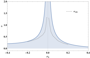
Refer to caption
Figure 8: Phase space for α𝛼\alpha and σhsubscript𝜎\sigma_{h} with fixed values of λ𝜆\lambda in the symmetry-broken phase

Within the parameter values in the phase space, we numerically generate hairy black hole solutions in the symmetry-broken phase with the same precision and accuracy used in the symmetric phase. For the choice of α=0.01𝛼0.01\alpha=0.01 with the fixed value of λ=0.1𝜆0.1\lambda=0.1, we plot the solutions in Figure 10 and Figure 10. By increasing the value of α𝛼\alpha, we observed that the numerical solutions become increasingly difficult to find for values of α𝛼\alpha exceeding αsolsubscript𝛼sol\alpha_{\textrm{sol}}, as discussed in [26].

Refer to caption
(a) The metric solutions with α=0.2𝛼0.2\alpha=0.2
Refer to caption
(b) ii
Refer to caption
(c) scalar field solutions
Figure 9: Hairy black hole solutions with σh=0.01subscript𝜎0.01\sigma_{h}=0.01 for various values of α𝛼\alpha. The black dotted line denotes the solutions of Schwarzschild black hole. The small regimes with the callout index (a)similar-to\sim(f) are plotted in Figure 10.
Refer to caption
(a) Case of α=0.2𝛼0.2\alpha=0.2
Refer to caption
(b) Case of α=0.2𝛼0.2\alpha=0.2
Refer to caption
(c) Case of α=0.2𝛼0.2\alpha=0.2
Refer to caption
(d) Case of α=0.6𝛼0.6\alpha=0.6
Refer to caption
(e) Case of α=0.6𝛼0.6\alpha=0.6
Refer to caption
(f) Case of α=0.6𝛼0.6\alpha=0.6
Figure 10: The comparison of metric solutions for hairy black holes and the Schwarzschild black hole. When α𝛼\alpha increases, hairy black holes exhibit a slight departure from the Schwarzschild black holes and show the anisotropic property of the metric (A/B1𝐴𝐵1A/B\neq 1). This deviation, though subtle, leads to noticeably distinct behavior in their QNMs for large α𝛼\alpha values.

6.2  Scalar Field Perturbation

We consider a linearized perturbation of the real scalar field as follows

σσ(z)+δσ(v,z,θ,ϕ).𝜎𝜎𝑧𝛿𝜎𝑣𝑧𝜃italic-ϕ\displaystyle\sigma\rightarrow\sigma(z)+\delta\sigma(v,z,\theta,\phi). (6.17)

Applying c2=0subscript𝑐20c_{2}=0 in (6.12) to the scalar field equations (6.6), the linearized part becomes

ααδσ+fσσ𝒢δσ=0.subscript𝛼superscript𝛼𝛿𝜎subscript𝑓𝜎𝜎𝒢𝛿𝜎0\displaystyle\nabla_{\alpha}\nabla^{\alpha}\delta\sigma+f_{\sigma\sigma}\mathcal{G}\delta\sigma=0. (6.18)

Using the following ansatz

δσ(v,z,θ,ϕ)=l,mΣ(z)Ylm(θ,ϕ)eiωv𝛿𝜎𝑣𝑧𝜃italic-ϕsubscript𝑙𝑚Σ𝑧subscript𝑌𝑙𝑚𝜃italic-ϕsuperscript𝑒𝑖𝜔𝑣\displaystyle\delta\sigma(v,z,\theta,\phi)=\sum_{l,m}\Sigma(z)Y_{lm}(\theta,\phi)e^{-i\omega v} (6.19)

and (5.19), the linearized equation is written as

z2A(z)B(z)Σ′′(z)+12(z2B(z)A(z)+z2A(z)B(z)+4iωB(z)A(z)B(z))Σ(z)superscript𝑧2𝐴𝑧𝐵𝑧superscriptΣ′′𝑧12superscript𝑧2𝐵𝑧superscript𝐴𝑧superscript𝑧2𝐴𝑧superscript𝐵𝑧4𝑖𝜔𝐵𝑧𝐴𝑧𝐵𝑧superscriptΣ𝑧\displaystyle z^{2}A(z)B(z)\Sigma^{\prime\prime}(z)+\frac{1}{2}\bigg{(}z^{2}B(z)A^{\prime}(z)+z^{2}A(z)B^{\prime}(z)+4i\omega B(z)\sqrt{\frac{A(z)}{B(z)}}\bigg{)}\Sigma^{\prime}(z) (6.20)
+1z2(A(z)(𝒢fσσ(σ)γz2)2iωzB(z)A(z)B(z))Σ(z)=0,1superscript𝑧2𝐴𝑧𝒢subscript𝑓𝜎𝜎𝜎𝛾superscript𝑧22𝑖𝜔𝑧𝐵𝑧𝐴𝑧𝐵𝑧Σ𝑧0\displaystyle+\frac{1}{z^{2}}\bigg{(}A(z)\left(\mathcal{G}f_{\sigma\sigma}(\sigma)-\gamma z^{2}\right)-2i\omega zB(z)\sqrt{\frac{A(z)}{B(z)}}\bigg{)}\Sigma(z)=0, (6.21)

where

fσσ(σ)=2α6αλσ3λσ2.subscript𝑓𝜎𝜎𝜎2𝛼6𝛼𝜆𝜎3𝜆superscript𝜎2\displaystyle f_{\sigma\sigma}(\sigma)=-2\alpha-6\sqrt{\alpha\lambda}\leavevmode\nobreak\ \sigma-3\lambda\sigma^{2}. (6.22)

The equation structure of (6.21) remains unchanged from (5.20). Thus we utilize (5.38), substituting f~φφsubscript~𝑓superscript𝜑𝜑\tilde{f}_{\varphi^{*}\varphi} with fσσsubscript𝑓𝜎𝜎f_{\sigma\sigma}, to test the instability of the QNMs.

6.3  Our Numerical Results

We employed the same strategy used in the symmetric phase to ensure the convergence of the eigenvalues. Calculations were performed on grids of 100100100 and 140140140, resulting in 100100100 and 140140140 eigenvalues, respectively. To identify reliable eigenvalues, we considered only those for which both the real and imaginary parts agreed within a tolerance of 102superscript10210^{-2} between the two grid sizes. Here, we only used hairy black hole solutions with a fixed value of λ=0.1𝜆0.1\lambda=0.1. To illustrate the behavior of quasinormal frequencies for varying α𝛼\alpha values, we first computed them for a background solution with σh=0.01subscript𝜎0.01\sigma_{h}=0.01. Representative results are presented for α=0.01,0.2,0.34𝛼0.010.20.34\alpha=0.01,0.2,0.34, and 0.380.380.38 in Figure 11, and for α=0.42,0.46,0.50,0.54,0.58,0.60,0.62𝛼0.420.460.500.540.580.600.62\alpha=0.42,0.46,0.50,0.54,0.58,0.60,0.62, and 0.660.660.66 in Figure 12. The numerical values for Figure 12 are presented in Appendix A. The QNM spectrum in Figure 12 for increasing positive values of α𝛼\alpha exhibits behaviors similar to those observed in Figure 5 for increasing negative values of α𝛼\alpha. Different from the symmetric phase with φh=0.01subscript𝜑0.01\varphi_{h}=0.01, the imaginary parts of quasinormal frequencies are all negative, which indicates the stability of hairy black holes. We also examined the quasinormal frequencies for σh=0.1subscript𝜎0.1\sigma_{h}=0.1 and plotted them for various values of α𝛼\alpha (α=0.01,0.1,0.2𝛼0.010.10.2\alpha=0.01,0.1,0.2, and 0.220.220.22) in Figure 13, which shows all negative values for the imaginary parts of quasinormal frequencies. We further investigated the quasinormal frequencies with the background solutions with σh=0.01subscript𝜎0.01\sigma_{h}=-0.01 and σh=0.1subscript𝜎0.1\sigma_{h}=-0.1 for various values of α𝛼\alpha. It turns out that they are stable for the linear scalar perturbation and the quasinormal frequencies.
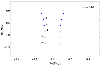
Refer to caption
Re[Mωn𝑀subscript𝜔𝑛M\omega_{n}] Im[Mωn𝑀subscript𝜔𝑛M\omega_{n}]
1 ±0.12229plus-or-minus0.12229\pm 0.12229 0.107010.10701-0.10701
2 ±0.10025plus-or-minus0.10025\pm 0.10025 0.350770.35077-0.35077
3 ±0.09104plus-or-minus0.09104\pm 0.091{\color[rgb]{.5,.5,.5}04} 0.603120.60312-0.603{\color[rgb]{.5,.5,.5}12}
4 ±0.08662plus-or-minus0.08662\pm 0.08{\color[rgb]{.5,.5,.5}662} 0.854480.85448-0.85{\color[rgb]{.5,.5,.5}448}
5 ±0.08226plus-or-minus0.08226\pm 0.08{\color[rgb]{.5,.5,.5}226} 1.102051.10205-1.10{\color[rgb]{.5,.5,.5}205}
6 ±0.08295plus-or-minus0.08295\pm 0.08{\color[rgb]{.5,.5,.5}295} 1.352461.35246-1.35{\color[rgb]{.5,.5,.5}246}
Refer to caption
Re[Mωn𝑀subscript𝜔𝑛M\omega_{n}] Im[Mωn𝑀subscript𝜔𝑛M\omega_{n}]
1 ±0.27261plus-or-minus0.27261\pm 0.27261 0.130840.13084-0.13084
2 ±0.26325plus-or-minus0.26325\pm 0.26325 0.409690.40969-0.40969
3 ±0.27500plus-or-minus0.27500\pm 0.27500 0.694740.69474-0.69474
4 ±0.29492plus-or-minus0.29492\pm 0.29492 0.965870.96587-0.96587
5 ±0.31297plus-or-minus0.31297\pm 0.31297 1.228471.22847-1.22847
6 ±0.32848plus-or-minus0.32848\pm 0.3284{\color[rgb]{.5,.5,.5}8} 1.48651.4865-1.486{\color[rgb]{.5,.5,.5}5}
Refer to caption
Re[Mωn𝑀subscript𝜔𝑛M\omega_{n}] Im[Mωn𝑀subscript𝜔𝑛M\omega_{n}]
1 ±0.35393plus-or-minus0.35393\pm 0.35393 0.136100.13610-0.13610
2 ±0.35217plus-or-minus0.35217\pm 0.35217 0.416230.41623-0.41623
3 ±0.36116plus-or-minus0.36116\pm 0.36116 0.695700.69570-0.69570
4 ±0.37179plus-or-minus0.37179\pm 0.37179 0.965820.96582-0.96582
5 ±0.37610plus-or-minus0.37610\pm 0.37610 1.227161.22716-1.22716
6 ±0.36866plus-or-minus0.36866\pm 0.3686{\color[rgb]{.5,.5,.5}6} 1.471931.47193-1.4719{\color[rgb]{.5,.5,.5}3}
Refer to caption
Re[Mωn𝑀subscript𝜔𝑛M\omega_{n}] Im[Mωn𝑀subscript𝜔𝑛M\omega_{n}]
1 ±0.37538plus-or-minus0.37538\pm 0.37538 0.137310.13731-0.13731
2 ±0.37399plus-or-minus0.37399\pm 0.37399 0.418420.41842-0.41842
3 ±0.38069plus-or-minus0.38069\pm 0.38069 0.698780.69878-0.69878
4 ±0.38549plus-or-minus0.38549\pm 0.38549 0.971370.97137-0.97137
5 ±0.37156plus-or-minus0.37156\pm 0.37156 1.234821.23482-1.23482
6 ±0.34159plus-or-minus0.34159\pm 0.341{\color[rgb]{.5,.5,.5}59} 1.424651.42465-1.424{\color[rgb]{.5,.5,.5}65}
7 ±0.41624plus-or-minus0.41624\pm 0.41{\color[rgb]{.5,.5,.5}624} 1.622981.62298-1.62{\color[rgb]{.5,.5,.5}298}
\captionlistentry

[table]A table beside a figure
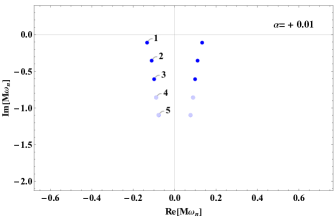
Figure 11: QNMs with various values of α𝛼\alpha for σh=0.01subscript𝜎0.01\sigma_{h}=0.01. Blue dots are tolerable less than 103superscript10310^{-3}, whereas lighter blue dots have a tolerance of 102superscript10210^{-2}.
Refer to caption

     Refer to caption

Refer to caption

     Refer to caption

Refer to caption

     Refer to caption

Refer to caption

     Refer to caption

Figure 12: QNMs with various values of α𝛼\alpha for σh=0.01subscript𝜎0.01\sigma_{h}=0.01. Blue dots are tolerable less than 103superscript10310^{-3}, whereas lighter blue dots have a tolerance of 102superscript10210^{-2}.
Refer to caption
Re[Mωn𝑀subscript𝜔𝑛M\omega_{n}] Im[Mωn𝑀subscript𝜔𝑛M\omega_{n}]
1 ±0.13296plus-or-minus0.13296\pm 0.13296 0.109150.10915-0.10915
2 ±0.11089plus-or-minus0.11089\pm 0.11089 0.354340.35434-0.35434
3 ±0.09888plus-or-minus0.09888\pm 0.098{\color[rgb]{.5,.5,.5}88} 0.607100.60710-0.607{\color[rgb]{.5,.5,.5}10}
4 ±0.08903plus-or-minus0.08903\pm 0.08{\color[rgb]{.5,.5,.5}903} 0.856840.85684-0.85{\color[rgb]{.5,.5,.5}684}
5 ±0.07694plus-or-minus0.07694\pm 0.07{\color[rgb]{.5,.5,.5}694} 1.096921.09692-1.09{\color[rgb]{.5,.5,.5}692}
Refer to caption
Re[Mωn𝑀subscript𝜔𝑛M\omega_{n}] Im[Mωn𝑀subscript𝜔𝑛M\omega_{n}]
1 ±0.23707plus-or-minus0.23707\pm 0.23707 0.128040.12804-0.12804
2 ±0.22250plus-or-minus0.22250\pm 0.22250 0.404290.40429-0.40429
3 ±0.23017plus-or-minus0.23017\pm 0.23017 0.689510.68951-0.68951
4 ±0.24834plus-or-minus0.24834\pm 0.24834 0.957230.95723-0.95723
5 ±0.26573plus-or-minus0.26573\pm 0.2657{\color[rgb]{.5,.5,.5}3} 1.212041.21204-1.2120{\color[rgb]{.5,.5,.5}4}
Refer to caption
Re[Mωn𝑀subscript𝜔𝑛M\omega_{n}] Im[Mωn𝑀subscript𝜔𝑛M\omega_{n}]
1 ±0.37969plus-or-minus0.37969\pm 0.37969 0.164320.16432-0.16432
2 ±0.33104plus-or-minus0.33104\pm 0.33104 0.510770.51077-0.51077
3 ±0.20870plus-or-minus0.20870\pm 0.20870 0.642080.64208-0.64208
4 ±0.35918plus-or-minus0.35918\pm 0.35918 0.895660.89566-0.89566
5 ±0.37078plus-or-minus0.37078\pm 0.37078 1.148741.14874-1.14874
6 ±0.41497plus-or-minus0.41497\pm 0.41497 1.362101.36210-1.36210
7 ±0.46862plus-or-minus0.46862\pm 0.4686{\color[rgb]{.5,.5,.5}2} 1.594951.59495-1.5949{\color[rgb]{.5,.5,.5}5}
8 ±0.51717plus-or-minus0.51717\pm 0.51{\color[rgb]{.5,.5,.5}717} 1.824241.82424-1.82{\color[rgb]{.5,.5,.5}424}
Refer to caption
Re[Mωn𝑀subscript𝜔𝑛M\omega_{n}] Im[Mωn𝑀subscript𝜔𝑛M\omega_{n}]
1 ±0.44235plus-or-minus0.44235\pm 0.44235 0.191320.19132-0.19132
2 ±0.40095plus-or-minus0.40095\pm 0.40095 0.609650.60965-0.60965
3 ±0.16308plus-or-minus0.16308\pm 0.16308 0.530550.53055-0.53055
4 ±0.36626plus-or-minus0.36626\pm 0.36626 0.950820.95082-0.95082
5 ±0.39292plus-or-minus0.39292\pm 0.39292 1.117521.11752-1.11752
6 ±0.46238plus-or-minus0.46238\pm 0.46238 1.369421.36942-1.36942
7 ±0.50981plus-or-minus0.50981\pm 0.5098{\color[rgb]{.5,.5,.5}1} 1.594441.59444-1.5944{\color[rgb]{.5,.5,.5}4}
8 ±0.57047plus-or-minus0.57047\pm 0.570{\color[rgb]{.5,.5,.5}47} 1.823791.82379-1.823{\color[rgb]{.5,.5,.5}79}
\captionlistentry

[table]A table beside a figure

Figure 13: QNMs with various values of α𝛼\alpha for σh=0.1subscript𝜎0.1\sigma_{h}=0.1. Blue dots are tolerable less than 103superscript10310^{-3}, whereas lighter blue dots have a tolerance of 102superscript10210^{-2}.

7.  Summary

We have argued that black holes without hairs grow their scalar hairs by spontaneous symmetry breaking under global U(1) symmetry in Einstein-scalar-Gauss-Bonnet theory, following the suggestion in [26]. We investigated the scalar field perturbation on the hairy black hole spacetimes to provide evidence for this process. We have fully analyzed the solution for the linearized scalar field equation by using Green’s function, which consists of three parts (GF,GBsubscript𝐺Fsubscript𝐺BG_{\textrm{F}},G_{\textrm{B}}, and GQNMsubscript𝐺QNMG_{\textrm{QNM}}). Our main focus was the calculation of QNMs (GQNMsubscript𝐺QNMG_{\textrm{QNM}}), which provides a powerful tool to study the stability of concerning systems. The branch cut contribution (GBsubscript𝐺BG_{\textrm{B}}) differs from the Schwarzschild black hole case only by the mass term. Since our hairy black hole solutions are numerically generated, we employed the numerical methods to compute the QNMs.

We firstly considered the Schwarzschild black hole, which is the solution without scalar fields, and examined the QNMs of scalar perturbation on this background. We found a critical point at which the imaginary part of the quasinormal frequency becomes positive, indicating the system’s instability. Then, we numerically constructed hairy black hole solutions in the symmetric and symmetry-broken phases. We assumed the scalar field always lies near the vacuum in each phase, so their near horizon values are small. Our calculations of the QNMs show that the hairy black holes in the symmetric phase also have a positive imaginary value of the quasinormal frequency at nearly the same critical point as the Schwarzschild black hole. However, the hairy black holes in the symmetry-broken phase always produce a negative imaginary value of the quasinormal frequency in the parameter ranges that we are concerned with. This numerical result indicates that the Schwarzschild black holes undergo a phase transition to the ones in the symmetry-broken phase by spontaneous symmetry breaking. Thus, their final stage through evolution becomes stable.

Our investigation focused on the scalar field perturbation within the probe limit, neglecting the potential backreaction on the metric. Since the background scalar field has a non-trivial contribution to the spacetime geometry, the perturbation itself will induce a corresponding change in that geometry. This backreaction effect can potentially influence the stability of the system. Thus, it is crucial to consider this effect in future work. Furthermore, studying the full non-linear time evolution of this process would be much more intriguing, but this work presents a significantly greater technical challenge.

Acknowledgments

B.L. and M.P. were supported by the Institute for Basic Science (Grant No. IBS-R018-Y1). Y.-H.H. was supported by Basic Science Research Program through the National Research Foundation of Korea (NRF) funded by the Ministry of Education (NRF-2021R1I1A2050775). We appreciate APCTP for its hospitality during completion of this work.

Appendix A. Numerical data for QNM

𝜶=0.2𝜶0.2\boldsymbol{\alpha=-0.2} 𝜶=0.8𝜶0.8\boldsymbol{\alpha=-0.8} 𝜶=0.9𝜶0.9\boldsymbol{\alpha=-0.9} 𝜶=𝟏𝜶1\boldsymbol{\alpha=-1}
Re[Mωn]Redelimited-[]𝑀subscript𝜔𝑛\mathrm{Re}[M\omega_{n}] Im[Mωn]Imdelimited-[]𝑀subscript𝜔𝑛\mathrm{Im}[M\omega_{n}] Re[Mωn]Redelimited-[]𝑀subscript𝜔𝑛\mathrm{Re}[M\omega_{n}] Im[Mωn]Imdelimited-[]𝑀subscript𝜔𝑛\mathrm{Im}[M\omega_{n}] Re[Mωn]Redelimited-[]𝑀subscript𝜔𝑛\mathrm{Re}[M\omega_{n}] Im[Mωn]Imdelimited-[]𝑀subscript𝜔𝑛\mathrm{Im}[M\omega_{n}] Re[Mωn]Redelimited-[]𝑀subscript𝜔𝑛\mathrm{Re}[M\omega_{n}] Im[Mωn]Imdelimited-[]𝑀subscript𝜔𝑛\mathrm{Im}[M\omega_{n}]
1 ±0.26768plus-or-minus0.26768\pm 0.26768 0.130590.13059-0.13059 ±0.38081plus-or-minus0.38081\pm 0.38081 0.140520.14052-0.14052 ±0.40992plus-or-minus0.40992\pm 0.40992 0.144370.14437-0.14437 ±0.44302plus-or-minus0.44302\pm 0.44302 0.150170.15017-0.15017
2 ±0.25648plus-or-minus0.25648\pm 0.25648 0.410050.41005-0.41005 ±0.37650plus-or-minus0.37650\pm 0.37650 0.428910.42891-0.42891 ±0.40404plus-or-minus0.40404\pm 0.40404 0.440130.44013-0.44013 ±0.43517plus-or-minus0.43517\pm 0.43517 0.458850.45885-0.45885
3 ±0.26784plus-or-minus0.26784\pm 0.26784 0.697730.69773-0.69773 ±0.37689plus-or-minus0.37689\pm 0.37689 0.717520.71752-0.71752 ±0.39674plus-or-minus0.39674\pm 0.39674 0.742200.74220-0.74220 ±0.43080plus-or-minus0.43080\pm 0.43080 0.787880.78788-0.78788
4 ±0.28846plus-or-minus0.28846\pm 0.28846 0.969950.96995-0.96995 ±0.35977plus-or-minus0.35977\pm 0.35977 1.000141.00014-1.00014 ±0.40838plus-or-minus0.40838\pm 0.40838 1.086731.08673-1.08673 ±0.17853plus-or-minus0.17853\pm 0.1785{\color[rgb]{.5,.5,.5}3} 0.845140.84514-0.8451{\color[rgb]{.5,.5,.5}4}
5 ±0.30676plus-or-minus0.30676\pm 0.30676 1.232781.23278-1.23278 ±0.30338plus-or-minus0.30338\pm 0.3033{\color[rgb]{.5,.5,.5}8} 1.174301.17430-1.1743{\color[rgb]{.5,.5,.5}0} ±0.23848plus-or-minus0.23848\pm 0.2384{\color[rgb]{.5,.5,.5}8} 0.982210.98221-0.9822{\color[rgb]{.5,.5,.5}1} ±0.46553plus-or-minus0.46553\pm 0.46553 1.111141.11114-1.11114
6 ±0.32221plus-or-minus0.32221\pm 0.322{\color[rgb]{.5,.5,.5}21} 1.490561.49056-1.490{\color[rgb]{.5,.5,.5}56} ±0.40795plus-or-minus0.40795\pm 0.4079{\color[rgb]{.5,.5,.5}5} 1.373201.37320-1.3732{\color[rgb]{.5,.5,.5}0} ±0.45992plus-or-minus0.45992\pm 0.45992 1.371581.37158-1.37158 ±0.47431plus-or-minus0.47431\pm 0.4743{\color[rgb]{.5,.5,.5}1} 1.393101.39310-1.3931{\color[rgb]{.5,.5,.5}0}
7 ±0.45789plus-or-minus0.45789\pm 0.45{\color[rgb]{.5,.5,.5}789} 1.632471.63247-1.63{\color[rgb]{.5,.5,.5}247} ±0.48216plus-or-minus0.48216\pm 0.48{\color[rgb]{.5,.5,.5}216} 1.628901.62890-1.62{\color[rgb]{.5,.5,.5}890} ±0.46557plus-or-minus0.46557\pm 0.46{\color[rgb]{.5,.5,.5}557} 1.588351.58835-1.58{\color[rgb]{.5,.5,.5}835}
𝜶=1.1𝜶1.1\boldsymbol{\alpha=-1.1} 𝜶=1.2𝜶1.2\boldsymbol{\alpha=-1.2} 𝜶=1.3𝜶1.3\boldsymbol{\alpha=-1.3} 𝜶=1.4𝜶1.4\boldsymbol{\alpha=-1.4}
Re[Mωn]Redelimited-[]𝑀subscript𝜔𝑛\mathrm{Re}[M\omega_{n}] Im[Mωn]Imdelimited-[]𝑀subscript𝜔𝑛\mathrm{Im}[M\omega_{n}] Re[Mωn]Redelimited-[]𝑀subscript𝜔𝑛\mathrm{Re}[M\omega_{n}] Im[Mωn]Imdelimited-[]𝑀subscript𝜔𝑛\mathrm{Im}[M\omega_{n}] Re[Mωn]Redelimited-[]𝑀subscript𝜔𝑛\mathrm{Re}[M\omega_{n}] Im[Mωn]Imdelimited-[]𝑀subscript𝜔𝑛\mathrm{Im}[M\omega_{n}] Re[Mωn]Redelimited-[]𝑀subscript𝜔𝑛\mathrm{Re}[M\omega_{n}] Im[Mωn]Imdelimited-[]𝑀subscript𝜔𝑛\mathrm{Im}[M\omega_{n}]
1 ±0.48383plus-or-minus0.48383\pm 0.48383 0.159200.15920-0.15920 ±0.53874plus-or-minus0.53874\pm 0.53874 0.173610.17361-0.17361 ±0.61923plus-or-minus0.61923\pm 0.61923 0.197500.19750-0.19750 ±0.74663plus-or-minus0.74663\pm 0.74663 0.239840.23984-0.23984
2 ±0.47526plus-or-minus0.47526\pm 0.47526 0.488780.48878-0.48878 ±0.53170plus-or-minus0.53170\pm 0.53170 0.533570.53357-0.53357 ±0.06431plus-or-minus0.06431\pm 0.06{\color[rgb]{.5,.5,.5}431} 0.536580.53658-0.53{\color[rgb]{.5,.5,.5}658} ±0.04872plus-or-minus0.04872\pm 0.048{\color[rgb]{.5,.5,.5}72} 0.448240.44824-0.448{\color[rgb]{.5,.5,.5}24}
3 ±0.12955plus-or-minus0.12955\pm 0.129{\color[rgb]{.5,.5,.5}55} 0.726870.72687-0.726{\color[rgb]{.5,.5,.5}87} ±0.09204plus-or-minus0.09204\pm 0.092{\color[rgb]{.5,.5,.5}04} 0.626740.62674-0.626{\color[rgb]{.5,.5,.5}74} ±0.61256plus-or-minus0.61256\pm 0.61256 0.601740.60174-0.60174 ±0.73275plus-or-minus0.73275\pm 0.73275 0.713630.71363-0.71363
4 ±0.48476plus-or-minus0.48476\pm 0.48476 0.835780.83578-0.83578 ±0.54299plus-or-minus0.54299\pm 0.54299 0.903300.90330-0.90330 ±0.62800plus-or-minus0.62800\pm 0.62800 1.016981.01698-1.01698
5 ±0.49622plus-or-minus0.49622\pm 0.49622 1.166381.16638-1.16638 ±0.31338plus-or-minus0.31338\pm 0.3133{\color[rgb]{.5,.5,.5}8} 1.164761.16476-1.1647{\color[rgb]{.5,.5,.5}6} ±0.24812plus-or-minus0.24812\pm 0.24{\color[rgb]{.5,.5,.5}812} 1.028331.02833-1.02{\color[rgb]{.5,.5,.5}833}
6 ±0.39443plus-or-minus0.39443\pm 0.3944{\color[rgb]{.5,.5,.5}3} 1.344861.34486-1.3448{\color[rgb]{.5,.5,.5}6} ±0.57314plus-or-minus0.57314\pm 0.57314 1.283801.28380-1.28380 ±0.64992plus-or-minus0.64992\pm 0.64{\color[rgb]{.5,.5,.5}992} 1.441871.44187-1.44{\color[rgb]{.5,.5,.5}187}
7 ±0.55151plus-or-minus0.55151\pm 0.5515{\color[rgb]{.5,.5,.5}1} 1.538221.53822-1.5382{\color[rgb]{.5,.5,.5}2} ±0.56313plus-or-minus0.56313\pm 0.563{\color[rgb]{.5,.5,.5}13} 1.609131.60913-1.609{\color[rgb]{.5,.5,.5}13}
8 ±0.58607plus-or-minus0.58607\pm 0.58{\color[rgb]{.5,.5,.5}607} 1.740281.74028-1.74{\color[rgb]{.5,.5,.5}028}
Table 1: φh=0.01subscript𝜑0.01\varphi_{h}=0.01 for Figure 5
𝜶=0.12𝜶0.12\boldsymbol{\alpha=0.12} 𝜶=0.1815𝜶0.1815\boldsymbol{\alpha=0.1815} 𝜶=0.6𝜶0.6\boldsymbol{\alpha=0.6} 𝜶=𝟏𝜶1\boldsymbol{\alpha=1}
Re[Mωn]Redelimited-[]𝑀subscript𝜔𝑛\mathrm{Re}[M\omega_{n}] Im[Mωn]Imdelimited-[]𝑀subscript𝜔𝑛\mathrm{Im}[M\omega_{n}] Re[Mωn]Redelimited-[]𝑀subscript𝜔𝑛\mathrm{Re}[M\omega_{n}] Im[Mωn]Imdelimited-[]𝑀subscript𝜔𝑛\mathrm{Im}[M\omega_{n}] Re[Mωn]Redelimited-[]𝑀subscript𝜔𝑛\mathrm{Re}[M\omega_{n}] Im[Mωn]Imdelimited-[]𝑀subscript𝜔𝑛\mathrm{Im}[M\omega_{n}] Re[Mωn]Redelimited-[]𝑀subscript𝜔𝑛\mathrm{Re}[M\omega_{n}] Im[Mωn]Imdelimited-[]𝑀subscript𝜔𝑛\mathrm{Im}[M\omega_{n}]
1 ±0.01134plus-or-minus0.01134\pm 0.011{\color[rgb]{.5,.5,.5}34} 0.058660.05866-0.058{\color[rgb]{.5,.5,.5}66} 00 +0.000040.00004+0.00004 00 +0.166880.16688+0.16688 00 +0.263440.26344+0.26344
2 ±0.03957plus-or-minus0.03957\pm 0.039{\color[rgb]{.5,.5,.5}57} 0.209000.20900-0.209{\color[rgb]{.5,.5,.5}00} ±0.06827plus-or-minus0.06827\pm 0.06827 0.196170.19617-0.19617 ±0.06536plus-or-minus0.06536\pm 0.06536 0.134210.13421-0.13421 ±0.01447plus-or-minus0.01447\pm 0.014{\color[rgb]{.5,.5,.5}47} 0.061150.06115-0.061{\color[rgb]{.5,.5,.5}15}
3 ±0.08812plus-or-minus0.08812\pm 0.0881{\color[rgb]{.5,.5,.5}2} 0.462320.46232-0.4623{\color[rgb]{.5,.5,.5}2} ±0.11016plus-or-minus0.11016\pm 0.11016 0.457750.45775-0.45775 ±0.10783plus-or-minus0.10783\pm 0.10783 0.456360.45636-0.45636 ±0.11981plus-or-minus0.11981\pm 0.1198{\color[rgb]{.5,.5,.5}1} 0.566830.56683-0.5668{\color[rgb]{.5,.5,.5}3}
4 ±0.11406plus-or-minus0.11406\pm 0.114{\color[rgb]{.5,.5,.5}06} 0.720430.72043-0.720{\color[rgb]{.5,.5,.5}43} ±0.13493plus-or-minus0.13493\pm 0.1349{\color[rgb]{.5,.5,.5}3} 0.718160.71816-0.7181{\color[rgb]{.5,.5,.5}6} ±0.12237plus-or-minus0.12237\pm 0.1223{\color[rgb]{.5,.5,.5}7} 0.724140.72414-0.7241{\color[rgb]{.5,.5,.5}4} ±0.17531plus-or-minus0.17531\pm 0.1753{\color[rgb]{.5,.5,.5}1} 0.864610.86461-0.8646{\color[rgb]{.5,.5,.5}1}
5 ±0.13301plus-or-minus0.13301\pm 0.133{\color[rgb]{.5,.5,.5}01} 0.977730.97773-0.977{\color[rgb]{.5,.5,.5}73} ±0.15346plus-or-minus0.15346\pm 0.1534{\color[rgb]{.5,.5,.5}6} 0.976640.97664-0.9766{\color[rgb]{.5,.5,.5}4} ±0.12874plus-or-minus0.12874\pm 0.128{\color[rgb]{.5,.5,.5}74} 0.976120.97612-0.976{\color[rgb]{.5,.5,.5}12} ±0.26764plus-or-minus0.26764\pm 0.26764 1.146781.14678-1.14678
6 ±0.14821plus-or-minus0.14821\pm 0.148{\color[rgb]{.5,.5,.5}21} 1.233721.23372-1.233{\color[rgb]{.5,.5,.5}72} ±0.16846plus-or-minus0.16846\pm 0.168{\color[rgb]{.5,.5,.5}46} 1.233481.23348-1.233{\color[rgb]{.5,.5,.5}48} ±0.16207plus-or-minus0.16207\pm 0.162{\color[rgb]{.5,.5,.5}07} 1.206611.20661-1.206{\color[rgb]{.5,.5,.5}61} ±0.33984plus-or-minus0.33984\pm 0.339{\color[rgb]{.5,.5,.5}84} 1.400291.40029-1.400{\color[rgb]{.5,.5,.5}29}
7 ±0.16124plus-or-minus0.16124\pm 0.16{\color[rgb]{.5,.5,.5}124} 1.489611.48961-1.48{\color[rgb]{.5,.5,.5}961} ±0.18124plus-or-minus0.18124\pm 0.18{\color[rgb]{.5,.5,.5}124} 1.489541.48954-1.48{\color[rgb]{.5,.5,.5}954} ±0.22061plus-or-minus0.22061\pm 0.22{\color[rgb]{.5,.5,.5}061} 1.445641.44564-1.44{\color[rgb]{.5,.5,.5}564}
𝜶=1.6𝜶1.6\boldsymbol{\alpha=1.6} 𝜶=2.1𝜶2.1\boldsymbol{\alpha=2.1} 𝜶=2.4𝜶2.4\boldsymbol{\alpha=2.4} 𝜶=2.8𝜶2.8\boldsymbol{\alpha=2.8}
Re[Mωn]Redelimited-[]𝑀subscript𝜔𝑛\mathrm{Re}[M\omega_{n}] Im[Mωn]Imdelimited-[]𝑀subscript𝜔𝑛\mathrm{Im}[M\omega_{n}] Re[Mωn]Redelimited-[]𝑀subscript𝜔𝑛\mathrm{Re}[M\omega_{n}] Im[Mωn]Imdelimited-[]𝑀subscript𝜔𝑛\mathrm{Im}[M\omega_{n}] Re[Mωn]Redelimited-[]𝑀subscript𝜔𝑛\mathrm{Re}[M\omega_{n}] Im[Mωn]Imdelimited-[]𝑀subscript𝜔𝑛\mathrm{Im}[M\omega_{n}] Re[Mωn]Redelimited-[]𝑀subscript𝜔𝑛\mathrm{Re}[M\omega_{n}] Im[Mωn]Imdelimited-[]𝑀subscript𝜔𝑛\mathrm{Im}[M\omega_{n}]
1 00 +0.374760.37476+0.37476 00 +0.451680.45168+0.45168 00 +0.493380.49338+0.49338 00 +0.545040.54504+0.54504
2 00 +0.079020.07902+0.07902 00 +0.160140.16014+0.16014 00 +0.202800.20280+0.20280 00 +0.255090.25509+0.25509
3 ±0.03952plus-or-minus0.03952\pm 0.0395{\color[rgb]{.5,.5,.5}2} 0.182120.18212-0.1821{\color[rgb]{.5,.5,.5}2} ±0.04238plus-or-minus0.04238\pm 0.0423{\color[rgb]{.5,.5,.5}8} 0.130770.13077-0.1307{\color[rgb]{.5,.5,.5}7} ±0.03315plus-or-minus0.03315\pm 0.0331{\color[rgb]{.5,.5,.5}5} 0.101070.10107-0.1010{\color[rgb]{.5,.5,.5}7} ±0.01146plus-or-minus0.01146\pm 0.011{\color[rgb]{.5,.5,.5}46} 0.054020.05402-0.054{\color[rgb]{.5,.5,.5}02}
4 ±0.13005plus-or-minus0.13005\pm 0.1300{\color[rgb]{.5,.5,.5}5} 0.568950.56895-0.5689{\color[rgb]{.5,.5,.5}5} ±0.10588plus-or-minus0.10588\pm 0.1058{\color[rgb]{.5,.5,.5}8} 0.596050.59605-0.5960{\color[rgb]{.5,.5,.5}5} ±0.10394plus-or-minus0.10394\pm 0.103{\color[rgb]{.5,.5,.5}94} 0.602310.60231-0.602{\color[rgb]{.5,.5,.5}31}
5 ±0.25477plus-or-minus0.25477\pm 0.25477 0.853340.85334-0.85334 ±0.27384plus-or-minus0.27384\pm 0.2738{\color[rgb]{.5,.5,.5}4} 0.818880.81888-0.8188{\color[rgb]{.5,.5,.5}8} ±0.27571plus-or-minus0.27571\pm 0.27{\color[rgb]{.5,.5,.5}571} 0.794580.79458-0.79{\color[rgb]{.5,.5,.5}458}
6 ±0.35290plus-or-minus0.35290\pm 0.35290 1.095061.09506-1.09506 ±0.38709plus-or-minus0.38709\pm 0.387{\color[rgb]{.5,.5,.5}09} 1.039061.03906-1.039{\color[rgb]{.5,.5,.5}06}
7 ±0.43797plus-or-minus0.43797\pm 0.4379{\color[rgb]{.5,.5,.5}7} 1.328631.32863-1.3286{\color[rgb]{.5,.5,.5}3}
Table 2: φh=0.01subscript𝜑0.01\varphi_{h}=0.01 for Figure 6
𝜶=0.42𝜶0.42\boldsymbol{\alpha=0.42} 𝜶=0.46𝜶0.46\boldsymbol{\alpha=0.46} 𝜶=0.5𝜶0.5\boldsymbol{\alpha=0.5} 𝜶=0.54𝜶0.54\boldsymbol{\alpha=0.54}
Re[Mωn]Redelimited-[]𝑀subscript𝜔𝑛\mathrm{Re}[M\omega_{n}] Im[Mωn]Imdelimited-[]𝑀subscript𝜔𝑛\mathrm{Im}[M\omega_{n}] Re[Mωn]Redelimited-[]𝑀subscript𝜔𝑛\mathrm{Re}[M\omega_{n}] Im[Mωn]Imdelimited-[]𝑀subscript𝜔𝑛\mathrm{Im}[M\omega_{n}] Re[Mωn]Redelimited-[]𝑀subscript𝜔𝑛\mathrm{Re}[M\omega_{n}] Im[Mωn]Imdelimited-[]𝑀subscript𝜔𝑛\mathrm{Im}[M\omega_{n}] Re[Mωn]Redelimited-[]𝑀subscript𝜔𝑛\mathrm{Re}[M\omega_{n}] Im[Mωn]Imdelimited-[]𝑀subscript𝜔𝑛\mathrm{Im}[M\omega_{n}]
1 ±0.39686plus-or-minus0.39686\pm 0.39686 0.138740.13874-0.13874 ±0.41901plus-or-minus0.41901\pm 0.41901 0.140610.14061-0.14061 ±0.44270plus-or-minus0.44270\pm 0.44270 0.143190.14319-0.14319 ±0.46922plus-or-minus0.46922\pm 0.46922 0.146850.14685-0.14685
2 ±0.39535plus-or-minus0.39535\pm 0.39535 0.421790.42179-0.42179 ±0.41703plus-or-minus0.41703\pm 0.41703 0.427070.42707-0.42707 ±0.44016plus-or-minus0.44016\pm 0.44016 0.435200.43520-0.43520 ±0.46650plus-or-minus0.46650\pm 0.46650 0.447370.44737-0.44737
3 ±0.39899plus-or-minus0.39899\pm 0.39899 0.705040.70504-0.70504 ±0.41731plus-or-minus0.41731\pm 0.41731 0.716680.71668-0.71668 ±0.43915plus-or-minus0.43915\pm 0.43915 0.736370.73637-0.73637 ±0.47048plus-or-minus0.47048\pm 0.47048 0.762960.76296-0.76296
4 ±0.39449plus-or-minus0.39449\pm 0.39449 0.986080.98608-0.98608 ±0.41082plus-or-minus0.41082\pm 0.41082 1.025621.02562-1.02562 ±0.45927plus-or-minus0.45927\pm 0.45927 1.055871.05587-1.05587 ±0.49901plus-or-minus0.49901\pm 0.49901 1.077151.07715-1.07715
5 ±0.40264plus-or-minus0.40264\pm 0.4026{\color[rgb]{.5,.5,.5}4} 1.337221.33722-1.3372{\color[rgb]{.5,.5,.5}2} ±0.46181plus-or-minus0.46181\pm 0.46181 1.335021.33502-1.33502 ±0.49551plus-or-minus0.49551\pm 0.49551 1.343391.34339-1.34339 ±0.50952plus-or-minus0.50952\pm 0.50952 1.37281.3728-1.3728
6 ±0.29529plus-or-minus0.29529\pm 0.2952{\color[rgb]{.5,.5,.5}9} 1.217761.21776-1.2177{\color[rgb]{.5,.5,.5}6} ±0.23952plus-or-minus0.23952\pm 0.2395{\color[rgb]{.5,.5,.5}2} 1.080011.08001-1.0800{\color[rgb]{.5,.5,.5}1} ±0.18462plus-or-minus0.18462\pm 0.184{\color[rgb]{.5,.5,.5}62} 0.948480.94848-0.948{\color[rgb]{.5,.5,.5}48} ±0.14511plus-or-minus0.14511\pm 0.145{\color[rgb]{.5,.5,.5}11} 0.836370.83637-0.836{\color[rgb]{.5,.5,.5}37}
7 ±0.46611plus-or-minus0.46611\pm 0.46{\color[rgb]{.5,.5,.5}611} 1.604761.60476-1.60{\color[rgb]{.5,.5,.5}476} ±0.49727plus-or-minus0.49727\pm 0.497{\color[rgb]{.5,.5,.5}27} 1.601011.60101-1.601{\color[rgb]{.5,.5,.5}01} ±0.50148plus-or-minus0.50148\pm 0.50{\color[rgb]{.5,.5,.5}148} 1.606791.60679-1.60{\color[rgb]{.5,.5,.5}679} ±0.43876plus-or-minus0.43876\pm 0.43{\color[rgb]{.5,.5,.5}876} 1.554361.55436-1.55{\color[rgb]{.5,.5,.5}436}
8 ±0.56580plus-or-minus0.56580\pm 0.56{\color[rgb]{.5,.5,.5}580} 1.735271.73527-1.73{\color[rgb]{.5,.5,.5}527}
𝜶=0.58𝜶0.58\boldsymbol{\alpha=0.58} 𝜶=0.6𝜶0.6\boldsymbol{\alpha=0.6} 𝜶=0.62𝜶0.62\boldsymbol{\alpha=0.62} 𝜶=0.66𝜶0.66\boldsymbol{\alpha=0.66}
Re[Mωn]Redelimited-[]𝑀subscript𝜔𝑛\mathrm{Re}[M\omega_{n}] Im[Mωn]Imdelimited-[]𝑀subscript𝜔𝑛\mathrm{Im}[M\omega_{n}] Re[Mωn]Redelimited-[]𝑀subscript𝜔𝑛\mathrm{Re}[M\omega_{n}] Im[Mωn]Imdelimited-[]𝑀subscript𝜔𝑛\mathrm{Im}[M\omega_{n}] Re[Mωn]Redelimited-[]𝑀subscript𝜔𝑛\mathrm{Re}[M\omega_{n}] Im[Mωn]Imdelimited-[]𝑀subscript𝜔𝑛\mathrm{Im}[M\omega_{n}] Re[Mωn]Redelimited-[]𝑀subscript𝜔𝑛\mathrm{Re}[M\omega_{n}] Im[Mωn]Imdelimited-[]𝑀subscript𝜔𝑛\mathrm{Im}[M\omega_{n}]
1 ±0.50045plus-or-minus0.50045\pm 0.50045 0.152120.15212-0.15212 ±0.51870plus-or-minus0.51870\pm 0.51870 0.155590.15559-0.15559 ±0.53936plus-or-minus0.53936\pm 0.53936 0.159790.15979-0.15979 ±0.59066plus-or-minus0.59066\pm 0.59066 0.171180.17118-0.17118
2 ±0.49861plus-or-minus0.49861\pm 0.49861 0.464930.46493-0.46493 ±0.51784plus-or-minus0.51784\pm 0.51784 0.476210.47621-0.47621 ±0.53981plus-or-minus0.53981\pm 0.53981 0.489510.48951-0.48951 ±0.59435plus-or-minus0.59435\pm 0.59435 0.524180.52418-0.52418
3 ±0.51056plus-or-minus0.51056\pm 0.51056 0.792580.79258-0.79258 ±0.53271plus-or-minus0.53271\pm 0.53271 0.810160.81016-0.81016 ±0.55678plus-or-minus0.55678\pm 0.55678 0.831410.83141-0.83141 ±0.61569plus-or-minus0.61569\pm 0.61569 0.890020.89002-0.89002
4 ±0.53295plus-or-minus0.53295\pm 0.53295 1.114121.11412-1.11412 ±0.55363plus-or-minus0.55363\pm 0.55363 1.144601.14460-1.14460 ±0.58299plus-or-minus0.58299\pm 0.58299 1.180301.18030-1.18030 ±0.65080plus-or-minus0.65080\pm 0.65080 1.261341.26134-1.26134
5 ±0.56587plus-or-minus0.56587\pm 0.56587 1.460741.46074-1.46074 ±0.59853plus-or-minus0.59853\pm 0.59853 1.484061.48406-1.48406 ±0.62056plus-or-minus0.62056\pm 0.62056 1.517451.51745-1.51745 ±0.69437plus-or-minus0.69437\pm 0.6943{\color[rgb]{.5,.5,.5}7} 1.643721.64372-1.6437{\color[rgb]{.5,.5,.5}2}
6 ±0.11391plus-or-minus0.11391\pm 0.113{\color[rgb]{.5,.5,.5}91} 0.738060.73806-0.738{\color[rgb]{.5,.5,.5}06} ±0.10044plus-or-minus0.10044\pm 0.100{\color[rgb]{.5,.5,.5}44} 0.693270.69327-0.693{\color[rgb]{.5,.5,.5}27} ±0.09007plus-or-minus0.09007\pm 0.090{\color[rgb]{.5,.5,.5}07} 0.652340.65234-0.652{\color[rgb]{.5,.5,.5}34} ±0.07204plus-or-minus0.07204\pm 0.07{\color[rgb]{.5,.5,.5}204} 0.577040.57704-0.57{\color[rgb]{.5,.5,.5}704}
7 ±0.36460plus-or-minus0.36460\pm 0.3646{\color[rgb]{.5,.5,.5}0} 1.362641.36264-1.3626{\color[rgb]{.5,.5,.5}4} ±0.32955plus-or-minus0.32955\pm 0.3295{\color[rgb]{.5,.5,.5}5} 1.285481.28548-1.2854{\color[rgb]{.5,.5,.5}8} ±0.29743plus-or-minus0.29743\pm 0.2974{\color[rgb]{.5,.5,.5}3} 1.210131.21013-1.2101{\color[rgb]{.5,.5,.5}3} ±0.24181plus-or-minus0.24181\pm 0.241{\color[rgb]{.5,.5,.5}81} 1.079901.07990-1.079{\color[rgb]{.5,.5,.5}90}
8 ±0.60883plus-or-minus0.60883\pm 0.60{\color[rgb]{.5,.5,.5}883} 1.753961.75396-1.75{\color[rgb]{.5,.5,.5}396} ±0.59270plus-or-minus0.59270\pm 0.59{\color[rgb]{.5,.5,.5}270} 1.780701.78070-1.78{\color[rgb]{.5,.5,.5}070} ±0.52726plus-or-minus0.52726\pm 0.52{\color[rgb]{.5,.5,.5}726} 1.743321.74332-1.74{\color[rgb]{.5,.5,.5}332} ±0.44858plus-or-minus0.44858\pm 0.4485{\color[rgb]{.5,.5,.5}8} 1.550201.55020-1.5502{\color[rgb]{.5,.5,.5}0}
Table 3: σh=1100subscript𝜎1100\sigma_{h}=\frac{1}{100} for Figure 12

Appendix B. Eigenfunctions

By examining the corresponding eigenfunctions, we confirm the physical validity of the QNM frequencies from our numerical data. We here demonstrate the eigenfunctions associated with the QNM frequencies which are computed on the hairy black holes with φh=0.01subscript𝜑0.01\varphi_{h}=0.01 at α=0.1815𝛼0.1815\alpha=0.1815 in Figure 14. We used the QNM frequencies with the positive real values and normalized the eigenfunctions to be 111 at the horizon. As we expected, all eigenfunctions are smooth and finite.
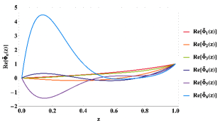
Refer to caption
Refer to caption
Figure 14: The eigenfunctions corresponding to the quasinormal frequencies of the hairy black hole with φh=0.01subscript𝜑0.01\varphi_{h}=0.01 at α=0.1815𝛼0.1815\alpha=0.1815 and λ=0.1𝜆0.1\lambda=0.1. The subscript of Φ~(z)~Φ𝑧\tilde{\Phi}(z) shares the same number of the QNM data presented in Table 6.

Appendix C. QNM with angular momentum

To investigate the dependence on angular momentum l𝑙l of the perturbed scalar field, we calculated quasinormal frequencies for various values l𝑙l. We employed a hairy black hole solution generated with specific parameters: φh=0.01subscript𝜑0.01\varphi_{h}=0.01, α=0.1815𝛼0.1815\alpha=0.1815, and λ=0.1𝜆0.1\lambda=0.1. The resulting QNM spectrum for l=0𝑙0l=0 to 555 and their numerical data are presented in Figure 15 and Table 8 respectively.
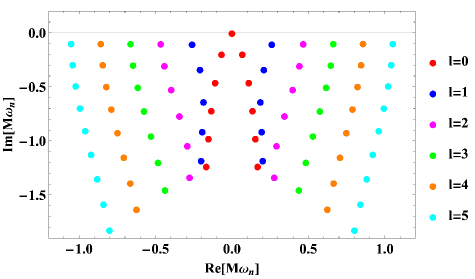
Refer to caption
𝒍=𝟎𝒍0\boldsymbol{l=0} 𝒍=𝟏𝒍1\boldsymbol{l=1} 𝒍=𝟐𝒍2\boldsymbol{l=2}
Re[Mωn]Redelimited-[]𝑀subscript𝜔𝑛\text{Re}[M\omega_{n}] Im[Mωn]Imdelimited-[]𝑀subscript𝜔𝑛\text{Im}[M\omega_{n}] Re[Mωn]Redelimited-[]𝑀subscript𝜔𝑛\text{Re}[M\omega_{n}] Im[Mωn]Imdelimited-[]𝑀subscript𝜔𝑛\text{Im}[M\omega_{n}] Re[Mωn]Redelimited-[]𝑀subscript𝜔𝑛\text{Re}[M\omega_{n}] Im[Mωn]Imdelimited-[]𝑀subscript𝜔𝑛\text{Im}[M\omega_{n}]
1 00 +0.000040.00004+0.00004 ±0.26085plus-or-minus0.26085\pm 0.26085 0.103280.10328-0.10328 ±0.46605plus-or-minus0.46605\pm 0.46605 0.098770.09877-0.09877
2 ±0.06827plus-or-minus0.06827\pm 0.06827 0.196170.19617-0.19617 ±0.20933plus-or-minus0.20933\pm 0.20933 0.337650.33765-0.33765 ±0.44129plus-or-minus0.44129\pm 0.44129 0.302350.30235-0.30235
3 ±0.11016plus-or-minus0.11016\pm 0.11016 0.457750.45775-0.45775 ±0.18652plus-or-minus0.18652\pm 0.18652 0.637110.63711-0.63711 ±0.39743plus-or-minus0.39743\pm 0.39743 0.522680.52268-0.52268
4 ±0.13493plus-or-minus0.13493\pm 0.13493 0.718160.71816-0.71816 ±0.19404plus-or-minus0.19404\pm 0.19404 0.912760.91276-0.91276 ±0.34352plus-or-minus0.34352\pm 0.34352 0.766350.76635-0.76635
5 ±0.15346plus-or-minus0.15346\pm 0.1534{\color[rgb]{.5,.5,.5}6} 0.976640.97664-0.9766{\color[rgb]{.5,.5,.5}4} ±0.20183plus-or-minus0.20183\pm 0.2018{\color[rgb]{.5,.5,.5}3} 1.180461.18046-1.1804{\color[rgb]{.5,.5,.5}6} ±0.29168plus-or-minus0.29168\pm 0.29168 1.042711.04271-1.04271
6 ±0.16846plus-or-minus0.16846\pm 0.168{\color[rgb]{.5,.5,.5}46} 1.233481.23348-1.233{\color[rgb]{.5,.5,.5}48} ±0.27697plus-or-minus0.27697\pm 0.2769{\color[rgb]{.5,.5,.5}7} 1.334031.33403-1.3340{\color[rgb]{.5,.5,.5}3}
𝒍=𝟑𝒍3\boldsymbol{l=3} 𝒍=𝟒𝒍4\boldsymbol{l=4} 𝒍=𝟓𝒍5\boldsymbol{l=5}
Re[Mωn]Redelimited-[]𝑀subscript𝜔𝑛\text{Re}[M\omega_{n}] Im[Mωn]Imdelimited-[]𝑀subscript𝜔𝑛\text{Im}[M\omega_{n}] Re[Mωn]Redelimited-[]𝑀subscript𝜔𝑛\text{Re}[M\omega_{n}] Im[Mωn]Imdelimited-[]𝑀subscript𝜔𝑛\text{Im}[M\omega_{n}] Re[Mωn]Redelimited-[]𝑀subscript𝜔𝑛\text{Re}[M\omega_{n}] Im[Mωn]Imdelimited-[]𝑀subscript𝜔𝑛\text{Im}[M\omega_{n}]
1 ±0.66314plus-or-minus0.66314\pm 0.66314 0.097550.09755-0.09755 ±0.85802plus-or-minus0.85802\pm 0.85802 0.097040.09704-0.09704 ±1.05198plus-or-minus1.05198\pm 1.05198 0.096770.09677-0.09677
2 ±0.64659plus-or-minus0.64659\pm 0.64659 0.295560.29556-0.29556 ±0.84552plus-or-minus0.84552\pm 0.84552 0.292850.29285-0.29285 ±1.04191plus-or-minus1.04191\pm 1.04191 0.291480.29148-0.29148
3 ±0.61574plus-or-minus0.61574\pm 0.61574 0.501910.50191-0.50191 ±0.82160plus-or-minus0.82160\pm 0.82160 0.493730.49373-0.49373 ±1.02237plus-or-minus1.02237\pm 1.02237 0.489590.48959-0.48959
4 ±0.57502plus-or-minus0.57502\pm 0.57502 0.720510.72051-0.72051 ±0.78845plus-or-minus0.78845\pm 0.78845 0.702510.70251-0.70251 ±0.99456plus-or-minus0.99456\pm 0.99456 0.693160.69316-0.69316
5 ±0.52974plus-or-minus0.52974\pm 0.52974 0.952460.95246-0.95246 ±0.74919plus-or-minus0.74919\pm 0.74919 0.920950.92095-0.92095 ±0.96030plus-or-minus0.96030\pm 0.96030 0.903800.90380-0.90380
6 ±0.48374plus-or-minus0.48374\pm 0.48374 1.196411.19641-1.19641 ±0.70719plus-or-minus0.70719\pm 0.70719 1.149311.14931-1.14931 ±0.92182plus-or-minus0.92182\pm 0.92182 1.122411.12241-1.12241
7 ±0.43825plus-or-minus0.43825\pm 0.4382{\color[rgb]{.5,.5,.5}5} 1.451111.45111-1.4511{\color[rgb]{.5,.5,.5}1} ±0.66516plus-or-minus0.66516\pm 0.66516 1.386501.38650-1.38650 ±0.88141plus-or-minus0.88141\pm 0.88141 1.349031.34903-1.34903
8 ±0.62465plus-or-minus0.62465\pm 0.6246{\color[rgb]{.5,.5,.5}5} 1.630761.63076-1.6307{\color[rgb]{.5,.5,.5}6} ±0.84101plus-or-minus0.84101\pm 0.84101 1.582921.58292-1.58292
9 ±0.80194plus-or-minus0.80194\pm 0.801{\color[rgb]{.5,.5,.5}94} 1.822891.82289-1.822{\color[rgb]{.5,.5,.5}89}
\captionlistentry

[table]A table beside a figure

Figure 15: The QNM frequencies for various values of l𝑙l. The background hairy black hole solution is employed for the case of φh=0.01,α=0.1815formulae-sequencesubscript𝜑0.01𝛼0.1815\varphi_{h}=0.01,\alpha=0.1815 and λ=0.1𝜆0.1\lambda=0.1.

References

  • [1] B. P. Abbott et al., “Observation of Gravitational Waves from a Binary Black Hole Merger,” Phys. Rev. Lett., vol. 116, no. 6, p. 061102, 2016.
  • [2] D. Clowe, M. Bradac, A. H. Gonzalez, M. Markevitch, S. W. Randall, C. Jones, and D. Zaritsky, “A direct empirical proof of the existence of dark matter,” Astrophys. J. Lett., vol. 648, pp. L109–L113, 2006.
  • [3] A. D. Linde, “Chaotic Inflation,” Phys. Lett. B, vol. 129, pp. 177–181, 1983.
  • [4] A. A. Starobinsky, “A New Type of Isotropic Cosmological Models Without Singularity,” Phys. Lett. B, vol. 91, pp. 99–102, 1980.
  • [5] D. Lovelock, “The Einstein tensor and its generalizations,” J. Math. Phys., vol. 12, pp. 498–501, 1971.
  • [6] T. Kobayashi, M. Yamaguchi, and J. Yokoyama, “Generalized G-inflation: Inflation with the most general second-order field equations,” Prog. Theor. Phys., vol. 126, pp. 511–529, 2011.
  • [7] E. J. Copeland, A. Padilla, and P. M. Saffin, “The cosmology of the Fab-Four,” JCAP, vol. 12, p. 026, 2012.
  • [8] E. Babichev, W. T. Emond, and S. Ramazanov, “Shrouded black holes in Einstein-Gauss-Bonnet gravity,” Phys. Rev. D, vol. 106, no. 6, p. 063524, 2022.
  • [9] P. Dorlis, N. E. Mavromatos, and S.-N. Vlachos, “Bypassing Bekenstein’s no-scalar-hair theorem without violating the energy conditions,” 5 2023.
  • [10] G. ’t Hooft and M. J. G. Veltman, “One loop divergencies in the theory of gravitation,” Ann. Inst. H. Poincare Phys. Theor. A, vol. 20, pp. 69–94, 1974.
  • [11] B. Zwiebach, “Curvature Squared Terms and String Theories,” Phys. Lett. B, vol. 156, pp. 315–317, 1985.
  • [12] D. J. Gross and J. H. Sloan, “The Quartic Effective Action for the Heterotic String,” Nucl. Phys. B, vol. 291, pp. 41–89, 1987.
  • [13] G. Antoniou, A. Bakopoulos, and P. Kanti, “Evasion of No-Hair Theorems and Novel Black-Hole Solutions in Gauss-Bonnet Theories,” Phys. Rev. Lett., vol. 120, no. 13, p. 131102, 2018.
  • [14] B.-H. Lee, W. Lee, and D. Ro, “Expanded evasion of the black hole no-hair theorem in dilatonic Einstein-Gauss-Bonnet theory,” Phys. Rev. D, vol. 99, no. 2, p. 024002, 2019.
  • [15] J. D. Bekenstein, “Transcendence of the law of baryon-number conservation in black hole physics,” Phys. Rev. Lett., vol. 28, pp. 452–455, 1972.
  • [16] J. D. Bekenstein, “Novel “no-scalar-hair” theorem for black holes,” Phys. Rev. D, vol. 51, no. 12, p. R6608, 1995.
  • [17] A. Papageorgiou, C. Park, and M. Park, “Rectifying no-hair theorems in Gauss-Bonnet theory,” Phys. Rev. D, vol. 106, no. 8, p. 084024, 2022.
  • [18] L. Capuano, L. Santoni, and E. Barausse, “Black hole hairs in scalar-tensor gravity and the lack thereof,” Phys. Rev. D, vol. 108, no. 6, p. 064058, 2023.
  • [19] H. O. Silva, J. Sakstein, L. Gualtieri, T. P. Sotiriou, and E. Berti, “Spontaneous scalarization of black holes and compact stars from a gauss-bonnet coupling,” Phys. Rev. Lett., vol. 120, p. 131104, Mar 2018.
  • [20] J. L. Blázquez-Salcedo, D. D. Doneva, J. Kunz, and S. S. Yazadjiev, “Radial perturbations of the scalarized Einstein-Gauss-Bonnet black holes,” Phys. Rev. D, vol. 98, no. 8, p. 084011, 2018.
  • [21] M. Minamitsuji and T. Ikeda, “Scalarized black holes in the presence of the coupling to Gauss-Bonnet gravity,” Phys. Rev. D, vol. 99, no. 4, p. 044017, 2019.
  • [22] C. F. B. Macedo, J. Sakstein, E. Berti, L. Gualtieri, H. O. Silva, and T. P. Sotiriou, “Self-interactions and Spontaneous Black Hole Scalarization,” Phys. Rev. D, vol. 99, no. 10, p. 104041, 2019.
  • [23] M. Minamitsuji and S. Mukohyama, “Instability of scalarized compact objects in Einstein-scalar-Gauss-Bonnet theories,” Phys. Rev. D, vol. 108, no. 2, p. 024029, 2023.
  • [24] G. Antoniou, C. F. B. Macedo, R. McManus, and T. P. Sotiriou, “Stable spontaneously-scalarized black holes in generalized scalar-tensor theories,” Phys. Rev. D, vol. 106, no. 2, p. 024029, 2022.
  • [25] B. Kleihaus, J. Kunz, T. Utermöhlen, and E. Berti, “Quadrupole instability of static scalarized black holes,” Phys. Rev. D, vol. 107, no. 8, p. L081501, 2023.
  • [26] B. Latosh and M. Park, “Hairy Black Holes by Spontaneous Symmetry Breaking,” 5 2023.
  • [27] L. Amendola and R. Barbieri, “Dark matter from an ultra-light pseudo-Goldsone-boson,” Phys. Lett. B, vol. 642, pp. 192–196, 2006.
  • [28] M. Frigerio, T. Hambye, and E. Masso, “Sub-GeV dark matter as pseudo-Goldstone from the seesaw scale,” Phys. Rev. X, vol. 1, p. 021026, 2011.
  • [29] T. Alanne, H. Gertov, F. Sannino, and K. Tuominen, “Elementary Goldstone Higgs boson and dark matter,” Phys. Rev. D, vol. 91, no. 9, p. 095021, 2015.
  • [30] B. F. Schutz and C. M. Will, “Black hole normal modes - A semianalytic approach,” The Astrophysical Journal, vol. 291, pp. L33–L36, Apr. 1985.
  • [31] S. Iyer and C. M. Will, “Black-hole normal modes: A wkb approach. i. foundations and application of a higher-order wkb analysis of potential-barrier scattering,” Phys. Rev. D, vol. 35, pp. 3621–3631, Jun 1987.
  • [32] S. Iyer, “Black-hole normal modes: A wkb approach. ii. schwarzschild black holes,” Phys. Rev. D, vol. 35, pp. 3632–3636, Jun 1987.
  • [33] S. Chandrasekhar and S. L. Detweiler, “The quasi-normal modes of the Schwarzschild black hole,” Proc. Roy. Soc. Lond. A, vol. 344, pp. 441–452, 1975.
  • [34] E. W. Leaver, “An Analytic representation for the quasi normal modes of Kerr black holes,” Proc. Roy. Soc. Lond. A, vol. 402, pp. 285–298, 1985.
  • [35] A. Jansen, “Overdamped modes in Schwarzschild-de Sitter and a Mathematica package for the numerical computation of quasinormal modes,” Eur. Phys. J. Plus, vol. 132, no. 12, p. 546, 2017.
  • [36] N. Andersson, “Evolving test fields in a black hole geometry,” Phys. Rev. D, vol. 55, pp. 468–479, 1997.
  • [37] C. Gundlach, R. H. Price, and J. Pullin, “Late time behavior of stellar collapse and explosions: 1. Linearized perturbations,” Phys. Rev. D, vol. 49, pp. 883–889, 1994.
  • [38] İ. T. Dolapçi, “Chebyshev collocation method for solving linear differential equations,” Mathematical and Computational Applications, vol. 9, no. 1, pp. 107–115, 2004.
  • [39] K. Xu, “The chebyshev points of the first kind,” Applied Numerical Mathematics, vol. 102, pp. 17–30, 2016.