Energy-based Hopfield Boosting for Out-of-Distribution Detection

Claus Hofmann    Simon Schmid    Bernhard Lehner    Daniel Klotz    Sepp Hochreiter
Abstract

Out-of-distribution (OOD) detection is critical when deploying machine learning models in the real world. Outlier exposure methods, which incorporate auxiliary outlier data in the training process, can drastically improve OOD detection performance compared to approaches without advanced training strategies. We introduce Hopfield Boosting, a boosting approach, which leverages modern Hopfield energy (MHE) to sharpen the decision boundary between the in-distribution and OOD data. Hopfield Boosting encourages the model to concentrate on hard-to-distinguish auxiliary outlier examples that lie close to the decision boundary between in-distribution and auxiliary outlier data. Our method achieves a new state-of-the-art in OOD detection with outlier exposure, improving the FPR95 metric from 2.28 to 0.92 on CIFAR-10 and from 11.76 to 7.94 on CIFAR-100.

hopfield, energy, ood, out-of-distribution, boosting, deep learning

1 Introduction

Out-of-distribution (OOD) detection is crucial when using machine learning systems in the real world. Deployed models will — sooner or later — encounter inputs that deviate from the training distribution. For example, a system trained to recognize music genres might also hear a sound clip of construction site noise. In the best case, a naive deployment can then result in overly confident predictions. In the worst case, we will get erratic model behavior and completely wrong predictions (Hendrycks & Gimpel, 2017). The purpose of OOD detection is to classify these examples as OOD, such that the system can then, for instance, notify users that no prediction is possible or trigger a manual investigation. In this paper we propose Hopfield Boosting, a novel OOD detection method that leverages the energy component of modern Hopfield networks (MHNs; Ramsauer et al., 2021) and advances the state-of-the-art of OOD detection.

Our method uses an auxiliary outlier data set (AUX) to boost the model’s OOD detection capacity. This allows the training process to learn a boundary around the in-distribution (ID) data, improving the performance at the OOD detection task. In summary, our contributions are as follows:

  1. 1.

    We propose Hopfield Boosting, an OOD detection approach that samples weak learners by using modern Hopfield energy (MHE; Ramsauer et al., 2021).

  2. 2.

    Hopfield Boosting achieves a new state-of-the-art in OOD detection. It improves the average false positive rate at 95% true positives (FPR95) from 2.28 to 0.92 on CIFAR-10 and from 11.38 to 7.94 on CIFAR-100.

  3. 3.

    We provide a theoretical background that motivates the suitability of Hopfield Boosting for OOD detection.
Refer to caption
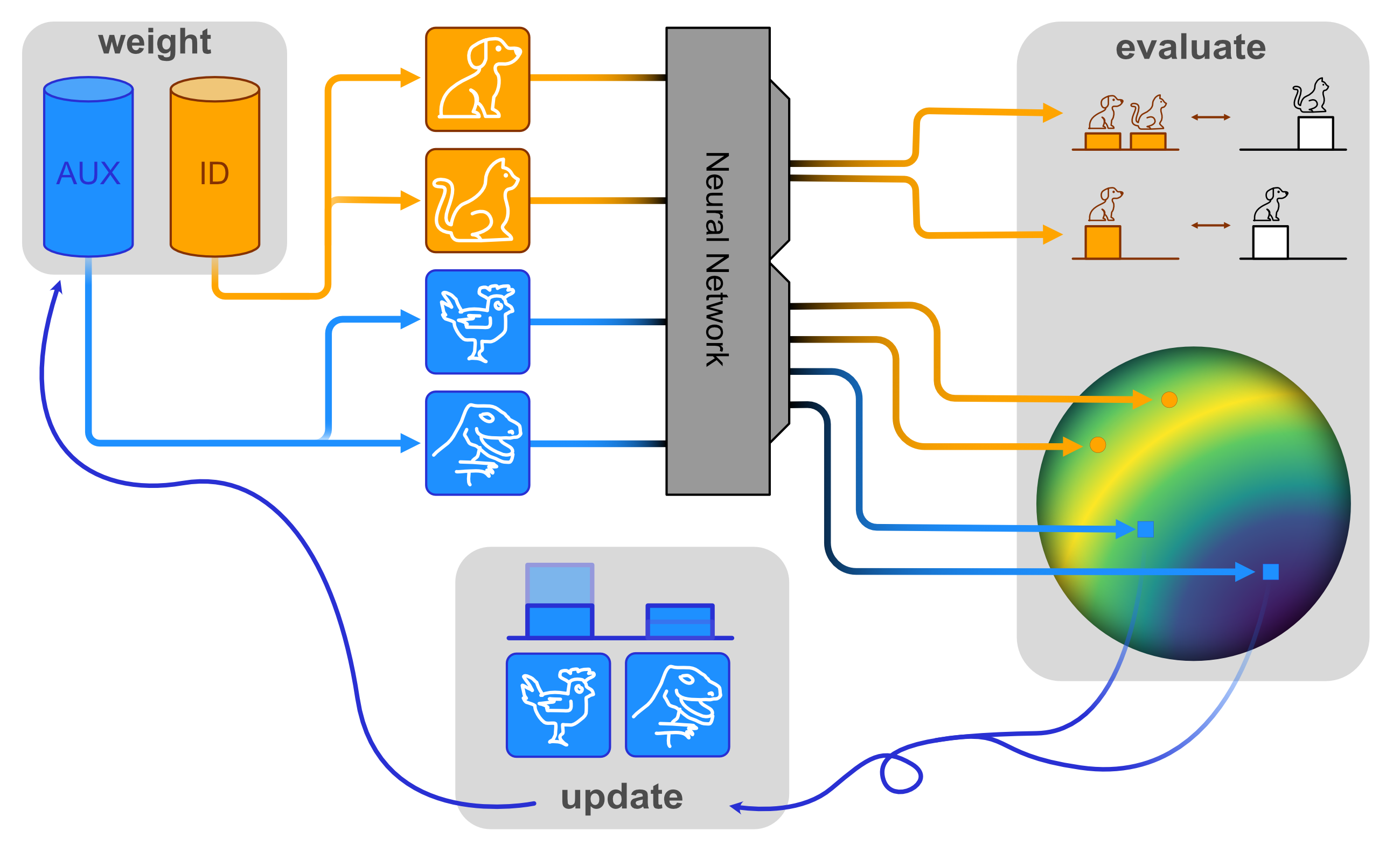
Figure 1: The Hopfield Boosting concept. The first step (weight) creates weak learners by firstly choosing in-distribution samples (ID, orange), and by secondly choosing auxiliary outlier samples (AUX, blue) according to their assigned probabilities; the second step (evaluate) computes the losses for the resulting predictions (Section 3); and the third step (update) assigns new probabilities to the AUX samples according to their position on the hypersphere (see Figure 2).

2 Related Work

Some authors (e.g., Bishop, 1994; Roth et al., 2022; Yang et al., 2022) distinguish between anomalies, outliers, and novelties. These distinctions reflect different goals within applications (Ruff et al., 2021). For example, when an anomaly is found, it will usually be removed from the training pipeline. However, when a novelty is found it should be studied. We focus on the detection of samples that are not part of the training distribution and consider sample categorization as a potential downstream task.

Post-hoc OOD detection.

A common and straightforward OOD detection approach is to use a post-hoc strategy, where one employs statistics obtained from a classifier. The perhaps most well known and simplest approach in this class is the Maximum Softmax Probability (MSP; Hendrycks & Gimpel, 2017), where one utilizes p(y|𝒙)𝑝conditional𝑦𝒙p(\ y\ |\ \bm{x}\ ) of the most likely class y𝑦y given a feature vector 𝒙D𝒙superscript𝐷\bm{x}\in\mathbb{R}^{D} to estimate whether a sample is OOD. Despite good empirical performances, this view is intrinsically limited, since OOD detection should to focus on p(𝒙)𝑝𝒙p(\bm{x}) (Morteza & Li, 2022). A wide range of post-hoc OOD detection approaches have been proposed to address the shortcomings of MSP (e.g., Lee et al., 2018; Liang et al., 2018; Hendrycks et al., 2019a; Liu et al., 2020; Huang et al., 2021; Sun et al., 2021, 2022; Wang et al., 2022; Sun et al., 2022; Sun & Li, 2022; Zhang et al., 2023a; Djurisic et al., 2023; Liu et al., 2023; Xu et al., 2024). Most related to Hopfield Boosting is the work of Zhang et al. (2023a), who, to our knowledge, are the first to apply MHE for OOD detection. Specifically, they propose a post-hoc OOD detection approach using MHE. They use the ID data set to produce stored patterns and then use a modified version of MHE as the OOD score. While post-hoc approaches can be deployed out of the box on any model, a crucial limitation is that their performance heavily depends on the employed model itself.

Training methods.

In contrast to post-hoc strategies, training-based methods modify the training process to improve the model’s OOD detection capability (e.g., Hendrycks et al., 2019c; Tack et al., 2020; Sehwag et al., 2021; Du et al., 2022; Hendrycks et al., 2022; Wei et al., 2022a; Ming et al., 2023; Tao et al., 2023; Lu et al., 2024). For example, Self-Supervised Outlier Detection (SSD; Sehwag et al., 2021) leverages contrastive self-supervised learning to train a model for OOD detection.

Auxiliary outlier data and outlier exposure.

A third group of OOD detection approaches are outlier exposure (OE) methods. Like Hopfield Boosting, they incorporate AUX data in the training process to improve the detection of OOD samples (e.g., Hendrycks et al., 2019b; Liu et al., 2020; Ming et al., 2022). As far as we know, all OE approaches optimize an objective (OODsubscriptOOD\mathcal{L}_{\text{OOD}}), which aims at improving the model’s discriminative power between ID and OOD data using the AUX data set as a stand-in for the OOD case. Hendrycks et al. (2019b) were the first to use the term OE to describe a more restrictive OE concept. Since their approach uses the MSP for incorporating the AUX data we refer to it as MSP-OE. Further, we refer to the OE approach introduced in Liu et al. (2020) as EBO-OE (to differentiate it from EBO, their post-hoc approach). In general, OE methods conceptualize the AUX data set as a large and diverse data set (e.g., ImageNet for vision tasks). As a consequence, usually, only a small subset of the samples bear semantic similarity to the ID data set — most data points are easily distinguishable from the ID data set. Recent approaches therefore actively try to find informative samples for the training. The aim is to refine the decision boundary, ensuring the ID data is more tightly encapsulated (e.g., Chen et al., 2021; Ming et al., 2022; Jiang et al., 2024). For example, Posterior Sampling-based Outlier Mining (POEM; Ming et al., 2022) selects samples close to the decision boundary using Thompson sampling: They first sample a linear decision boundary between ID and AUX data and then select those data instances which are closest to the sampled decision boundary. Hopfield Boosting also makes use of samples close to the boundary by giving them higher weights for the boosting step. Further OE methods include mixing-based OE methods (Zhang et al., 2023b; Zhu et al., 2023a), that employ mixup (Zhang et al., 2018) or CutMix (Yun et al., 2019) to augment the OE task. Distribution-Augmented OOD Learning (DAL; Wang et al., 2023a) augments the AUX data by defining a Wasserstein-1 ball around the AUX data and performing OE using this Wasserstein ball. Diversified Outlier Exposure (DivOE; Zhu et al., 2023b) synthesizes artificial auxiliary outliers, resulting in a more diverse coverage of the feature space. Distributional-agnostic Outlier Exposure (DOE; Wang et al., 2023b) implicitly synthesizes auxiliary outlier data using a transformation of the model weights, arguing that perturbing model parameters has the same effect as transforming the data. Diverse Outlier Sampling (DOS; Jiang et al., 2024) applies K-Means clustering to the features of the AUX data set and then samples outlier points close to the decision boundary uniformly from the obtained clusters. All mentioned OE-based methods were able to outperform their respective contemporary post-hoc or training approaches by a sizeable margin. This indicates that incorporating an appropriate AUX data set and applying OE during the training process improves the OOD detection capability in general.

Continuous modern Hopfield networks.

MHNs are energy-based associative memory networks. They advance conventional Hopfield networks (Hopfield, 1984) by introducing continuous queries and states with the MHE as a new energy function. MHE leads to exponential storage capacity, while retrieval is possible with a one-step update (Ramsauer et al., 2021). The update rule of MHNs coincides with the softmax-attention as it is used in the Transformer (Vaswani et al., 2017). Examples for successful applications of MHNs are Widrich et al. (2020); Fürst et al. (2022); Sanchez-Fernandez et al. (2022); Paischer et al. (2022); Schäfl et al. (2022) and Auer et al. (2023). Section 3.2 gives an introduction to MHE for OOD detection. For further details on MHNs, we refer to Appendix A.

Boosting for classification.

Boosting, in particular, AdaBoost (Freund & Schapire, 1995), is an ensemble learning technique for classification. It is designed to focus ensemble members toward data instances that are hard to classify by assigning them higher weights. These challenging instances often lie near the maximum margin hyperplane (Rätsch et al., 2001), akin to support vectors in support vector machines (SVMs; Cortes & Vapnik, 1995). Popular boosting methods include Gradient boosting (Breiman, 1997), LogitBoost (Friedman et al., 2000), and LPBoost (Demiriz et al., 2002).

Radial basis function networks.

Radial basis function networks (RBF networks; Moody & Darken, 1989) are function approximators of the form

φ(𝝃)=i=1Nωiexp(𝝃𝝁i222σi2),𝜑𝝃superscriptsubscript𝑖1𝑁subscript𝜔𝑖superscriptsubscriptnorm𝝃subscript𝝁𝑖222superscriptsubscript𝜎𝑖2\displaystyle\varphi(\bm{\xi})=\sum_{i=1}^{N}\omega_{i}\exp\left(-\frac{||\bm{\xi}-\bm{\mu}_{i}||_{2}^{2}}{2\sigma_{i}^{2}}\right), (1)

where ωisubscript𝜔𝑖\omega_{i} are linear weights, 𝝁isubscript𝝁𝑖\bm{\mu}_{i} are the component means and σi2subscriptsuperscript𝜎2𝑖\sigma^{2}_{i} are the component variances. RBF networks can be described as a weighted linear superposition of N𝑁N radial basis functions and have previously been used as hypotheses for boosting (Rätsch et al., 2001). If the linear weights are strictly positive, RBF networks can be viewed as an unnormalized weighted mixture of Gaussian distributions pi(𝝃)=𝒩(𝝃;𝝁i,σi2𝑰)subscript𝑝𝑖𝝃𝒩𝝃subscript𝝁𝑖superscriptsubscript𝜎𝑖2𝑰p_{i}(\bm{\xi})=\mathcal{N}(\bm{\xi};\bm{\mu}_{i},\sigma_{i}^{2}\bm{I}) with i={1,,N}𝑖1𝑁i=\{1,\dots,N\}. Appendix E.1 explores the connection between RBF networks and MHNs via Gaussian mixtures in more depth. We refer to Bishop (1995) and Müller et al. (1997) for more general information on RBF networks.

3 Method

This section presents Hopfield Boosting: First, we formalize the OOD detection task. Second, we give an overview of MHE and why it is suitable for OOD detection. Finally, we introduce the AUX-based boosting framework. Figure 1 shows a summary of the Hopfield Boosting concept.

3.1 Classification and OOD Detection

Consider a multi-class classification problem denoted as (𝑿𝒟,𝒀𝒟,𝒴)superscript𝑿𝒟superscript𝒀𝒟𝒴(\bm{X}^{\mathcal{D}},\bm{Y}^{\mathcal{D}},\mathcal{Y}), where 𝑿𝒟D×Nsuperscript𝑿𝒟superscript𝐷𝑁\bm{X}^{\mathcal{D}}\in\mathbb{R}^{D\times N} represents a set of N𝑁N D𝐷D-dimensional feature vectors (𝒙1𝒟,𝒙2𝒟,,𝒙N𝒟subscriptsuperscript𝒙𝒟1subscriptsuperscript𝒙𝒟2subscriptsuperscript𝒙𝒟𝑁\bm{x}^{\mathcal{D}}_{1},\bm{x}^{\mathcal{D}}_{2},\dots,\bm{x}^{\mathcal{D}}_{N}), which are i.i.d. samples 𝒙i𝒟pIDsimilar-tosuperscriptsubscript𝒙𝑖𝒟subscript𝑝ID\bm{x}_{i}^{\mathcal{D}}\sim p_{\text{ID}}. 𝒀𝒟𝒴Nsuperscript𝒀𝒟superscript𝒴𝑁\bm{Y}^{\mathcal{D}}\in\mathcal{Y}^{N} corresponds to the labels associated with these feature vectors, and 𝒴𝒴\mathcal{Y} is a set containing possible classes (𝒴=Knorm𝒴𝐾||\mathcal{Y}||=K signifies the number of distinct classes present).

We consider observations 𝝃𝒟Dsuperscript𝝃𝒟superscript𝐷\bm{\xi}^{\mathcal{D}}\in\mathbb{R}^{D} that deviate considerably from the data generation pID(𝝃𝒟)subscript𝑝IDsuperscript𝝃𝒟p_{\text{ID}}(\bm{\xi}^{\mathcal{D}}) that defines the “normality” of our data as OOD. Following Ruff et al. (2021), an observation is OOD if it pertains to the set

𝕆={𝝃𝒟D|pID(𝝃𝒟)<ϵ}whereϵ0.𝕆conditional-setsuperscript𝝃𝒟superscript𝐷subscript𝑝IDsuperscript𝝃𝒟italic-ϵwhereitalic-ϵ0\mathbb{O}\ =\ \{\bm{\xi}^{\mathcal{D}}\in\mathbb{R}^{D}\ |\ p_{\text{ID}}(\bm{\xi}^{\mathcal{D}})<\epsilon\}\ \text{where}\ \epsilon\geq 0. (2)

Since the probability density of the data generation pIDsubscript𝑝IDp_{\text{ID}} is in general not known, one needs to estimate pID(𝝃𝒟)subscript𝑝IDsuperscript𝝃𝒟p_{\text{ID}}(\bm{\xi}^{\mathcal{D}}). In practice, it is common to define an outlier score s(𝝃)𝑠𝝃s(\bm{\xi}) that uses an encoder ϕitalic-ϕ\phi, where 𝝃=ϕ(𝝃𝒟)𝝃italic-ϕsuperscript𝝃𝒟\bm{\xi}=\phi(\bm{\xi}^{\mathcal{D}}). The outlier score should — in the best case — preserve the density ranking.

In contrast to a density estimation, the score s(𝝃)𝑠𝝃s(\bm{\xi}) does not have to fulfill all requirements of a probability density (like proper normalization or non-negativity). Given s(𝝃)𝑠𝝃s(\bm{\xi}) and ϕitalic-ϕ\phi, OOD detection can be formulated as a binary classification task with the classes ID and OOD:

B^(𝝃𝒟,γ)={IDif s(ϕ(𝝃𝒟))γOODif s(ϕ(𝝃𝒟))<γ.^𝐵superscript𝝃𝒟𝛾casesIDif 𝑠italic-ϕsuperscript𝝃𝒟𝛾OODif 𝑠italic-ϕsuperscript𝝃𝒟𝛾\hat{B}(\bm{\xi}^{\mathcal{D}},\gamma)\ =\ \begin{cases}\text{ID}&\text{if }s(\phi(\bm{\xi}^{\mathcal{D}}))\geq\gamma\\ \text{OOD}&\text{if }s(\phi(\bm{\xi}^{\mathcal{D}}))<\gamma\\ \end{cases}. (3)

It is common to choose the threshold γ𝛾\gamma so that a portion of 95% of ID samples from a previously unseen validation set are correctly classified as ID. However, metrics like the area under the receiver operating characteristic (AUROC) can be directly computed on s(𝝃)𝑠𝝃s(\bm{\xi}) without specifying γ𝛾\gamma since the AUROC computation sweeps over the threshold.

3.2 Modern Hopfield Energy

The log-sum-exponential (lselse\mathrm{lse}) is defined as

lse(β,𝒛)=β1log(i=1Nexp(βzi)),lse𝛽𝒛superscript𝛽1superscriptsubscript𝑖1𝑁𝛽subscript𝑧𝑖\mathrm{lse}(\beta,\bm{z})=\ \beta^{-1}\ \log\left(\sum_{i=1}^{N}\exp(\beta z_{i})\right), (4)

where β𝛽\beta is the inverse temperature and 𝒛N𝒛superscript𝑁\bm{z}\in\mathbb{R}^{N} is a vector. The lselse\mathrm{lse} can be seen as a soft approximation to the maximum function: As β𝛽\beta\rightarrow\infty, the lselse\mathrm{lse} approaches maxizisubscript𝑖subscript𝑧𝑖\max_{i}z_{i}.

Given a set of N𝑁N d𝑑d-dimensional stored patterns (𝒙1,𝒙2,,𝒙N)subscript𝒙1subscript𝒙2subscript𝒙𝑁(\bm{x}_{1},\bm{x}_{2},\dots,\bm{x}_{N}) arranged in a data matrix 𝑿𝑿\bm{X}, and a d𝑑d-dimensional query 𝝃𝝃\bm{\xi}, the MHE is defined as

E(𝝃;𝑿)=lse(β,𝑿T𝝃)+12𝝃T𝝃+C,E𝝃𝑿lse𝛽superscript𝑿𝑇𝝃12superscript𝝃𝑇𝝃𝐶\mathrm{E}(\bm{\xi};\bm{X})\ =\ -\ \mathrm{lse}(\beta,\bm{X}^{T}\bm{\xi})+\ \frac{1}{2}\ \bm{\xi}^{T}\bm{\xi}\ +\ C, (5)

where C=β1logN+12M2𝐶superscript𝛽1𝑁12superscript𝑀2C=\beta^{-1}\log N\ +\frac{1}{2}M^{2} and M𝑀M is the largest norm of a pattern: M=maxixi𝑀subscript𝑖normsubscript𝑥𝑖M=\max_{i}||x_{i}||. For a fixed data matrix 𝑿𝑿\bm{X}, C𝐶C remains constant for any given query 𝝃𝝃\bm{\xi}. 𝑿𝑿\bm{X} is also called the memory of the MHN. Intuitively, Equation (5) can be explained as follows: The dot-product within the lselse\mathrm{lse} computes a similarity for a given 𝝃d𝝃superscript𝑑\bm{\xi}\in\mathbb{R}^{d} to all patterns in the memory 𝑿d×N𝑿superscript𝑑𝑁\bm{X}\in\mathbb{R}^{d\times N}. The lselse\mathrm{lse} function aggregates the similarities to form a single value. The parameter β𝛽\beta controls how the similarities are aggregated. If β𝛽\beta\rightarrow\infty, the similarity of 𝝃𝝃\bm{\xi} to the closest pattern in 𝑿𝑿\bm{X} is returned. Tuning β𝛽\beta allows one to adjust the “softness” of the lselse\mathrm{lse}. We can regard E(𝝃;𝑿)E𝝃𝑿\mathrm{E}(\bm{\xi};\bm{X}) as an expression of dissimilarity between 𝑿𝑿\bm{X} and 𝝃𝝃\bm{\xi}: If 𝝃𝝃\bm{\xi} is similar to 𝑿𝑿\bm{X}, E(𝝃;𝑿)E𝝃𝑿\mathrm{E}(\bm{\xi};\bm{X}) will be low. In contrast, if 𝝃𝝃\bm{\xi} is dissimilar from 𝑿𝑿\bm{X}, E(𝝃;𝑿)E𝝃𝑿\mathrm{E}(\bm{\xi};\bm{X}) will be high.

To use MHE for OOD detection, one needs a memory 𝑿𝑿\bm{X} of patterns from the ID data set. Hopfield Boosting acquires the memory patterns in 𝑿𝑿\bm{X} by feeding raw data instances (𝒙1𝒟,𝒙2𝒟,,𝒙N𝒟)subscriptsuperscript𝒙𝒟1subscriptsuperscript𝒙𝒟2subscriptsuperscript𝒙𝒟𝑁(\bm{x}^{\mathcal{D}}_{1},\bm{x}^{\mathcal{D}}_{2},\dots,\bm{x}^{\mathcal{D}}_{N}) arranged in the data matrix 𝑿𝒟superscript𝑿𝒟\bm{X}^{\mathcal{D}} of the ID data set to an encoder ϕ:Dd:italic-ϕsuperscript𝐷superscript𝑑\phi:\mathbb{R}^{D}\rightarrow\mathbb{R}^{d} (e.g., ResNet): 𝒙i=ϕ(𝒙i𝒟)subscript𝒙𝑖italic-ϕsubscriptsuperscript𝒙𝒟𝑖\bm{x}_{i}=\phi(\bm{x}^{\mathcal{D}}_{i}). We denote this component-wise application of an encoder to obtain a memory matrix as 𝑿=ϕ(𝑿𝒟)𝑿italic-ϕsuperscript𝑿𝒟\bm{X}=\phi(\bm{X}^{\mathcal{D}}). Similarly, a raw query 𝝃𝒟superscript𝝃𝒟\bm{\xi}^{\mathcal{D}} is fed through the encoder to obtain the query pattern: 𝝃=ϕ(𝝃𝒟)𝝃italic-ϕsuperscript𝝃𝒟\bm{\xi}=\phi(\bm{\xi}^{\mathcal{D}}). One can now use E(𝝃;𝑿)E𝝃𝑿\mathrm{E}(\bm{\xi};\bm{X}) to estimate whether 𝝃𝝃\bm{\xi} is ID or OOD: A low energy indicates 𝝃𝝃\bm{\xi} is ID, and a high energy signifies that 𝝃𝝃\bm{\xi} is OOD.

3.3 Boosting Framework

Sampling of informative outlier data.

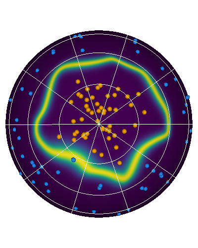
Hopfield Boosting uses an AUX data set to learn a decision boundary between the ID and OOD region during the training process. Similar to Chen et al. (2021) and Ming et al. (2022), Hopfield Boosting selects informative outliers close to the ID-OOD decision boundary and uses them for training the model. For this selection, Hopfield Boosting weights the AUX data similar to AdaBoost (Freund & Schapire, 1995) by sampling data instances close to the decision boundary more frequently. We consider samples close to the decision boundary as weak learners — their nearest neighbors consist of samples from their own class as well as from the foreign class. An individual weak learner would yield a classifier that is only slightly better than random guessing (Figure 7). Vice versa, a strong learner can be created by forming an ensemble of a set of weak learners (Figure 2).

We denote the matrix containing the raw AUX data instances (𝒐1𝒟,𝒐2𝒟,,𝒐N𝒟)subscriptsuperscript𝒐𝒟1subscriptsuperscript𝒐𝒟2subscriptsuperscript𝒐𝒟𝑁(\bm{o}^{\mathcal{D}}_{1},\bm{o}^{\mathcal{D}}_{2},\dots,\bm{o}^{\mathcal{D}}_{N}) as 𝑶𝒟D×Msuperscript𝑶𝒟superscript𝐷𝑀\bm{O}^{\mathcal{D}}\in\mathbb{R}^{D\times M}, and the memory containing the encoded AUX patterns as 𝑶=ϕ(𝑶𝒟)𝑶italic-ϕsuperscript𝑶𝒟\bm{O}=\phi(\bm{O}^{\mathcal{D}}). The boosting process proceeds as follows: There exists a weight (w1,w2,,wN)subscript𝑤1subscript𝑤2subscript𝑤𝑁(w_{1},w_{2},\dots,w_{N}) for each data point in 𝑶𝒟superscript𝑶𝒟\bm{O}^{\mathcal{D}} and the individual weights are aggregated into the weight vector 𝒘tsubscript𝒘𝑡\bm{w}_{t}. Hopfield Boosting uses these weights to draw mini-batches 𝑶s𝒟superscriptsubscript𝑶𝑠𝒟\bm{O}_{s}^{\mathcal{D}} from 𝑶𝒟superscript𝑶𝒟\bm{O}^{\mathcal{D}} for training, where weak learners are sampled more frequently into the Hopfield memory.

We introduce an MHE-based energy function which Hopfield Boosting uses to determine how weak a specific learner 𝝃𝝃\bm{\xi} is (with higher energy indicating a weaker learner):

Eb(𝝃;𝑿,𝑶)= 2lse(β,(𝑿𝑶)T𝝃)+lse(β,𝑿T𝝃)+lse(β,𝑶T𝝃),subscriptE𝑏𝝃𝑿𝑶2lse𝛽superscript𝑿𝑶𝑇𝝃lse𝛽superscript𝑿𝑇𝝃lse𝛽superscript𝑶𝑇𝝃\displaystyle\begin{split}\mathrm{E}_{b}(\bm{\xi};\bm{X},\bm{O})\ =\ -\ 2\ &\mathrm{lse}(\beta,(\bm{X}\mathbin{\|}\bm{O})^{T}\bm{\xi})\ +\\ \ &\mathrm{lse}(\beta,\bm{X}^{T}\bm{\xi})\ +\ \mathrm{lse}(\beta,\bm{O}^{T}\bm{\xi}),\end{split} (6)

where 𝑿d×N𝑿superscript𝑑𝑁\bm{X}\in\mathbb{R}^{d\times N} contains ID patterns, 𝑶d×M𝑶superscript𝑑𝑀\bm{O}\in\mathbb{R}^{d\times M} contains AUX patterns, and (𝑿𝑶)d×(N+M)𝑿𝑶superscript𝑑𝑁𝑀(\bm{X}\mathbin{\|}\bm{O})\in\mathbb{R}^{d\times(N+M)} denotes the concatenated data matrix containing the patterns from both 𝑿𝑿\bm{X} and 𝑶𝑶\bm{O}. Before computing EbsubscriptE𝑏\mathrm{E}_{b}, we normalize the feature vectors in 𝑿𝑿\bm{X}, 𝑶𝑶\bm{O}, and 𝝃𝝃\bm{\xi} to unit length.

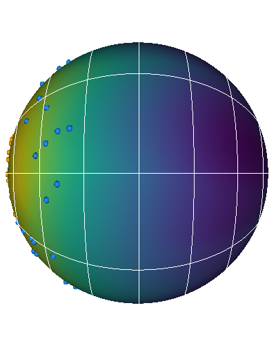
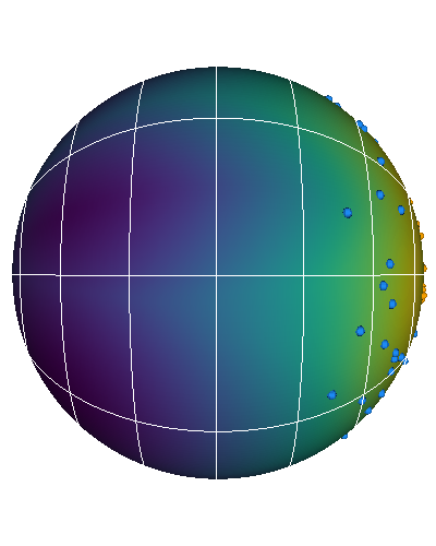
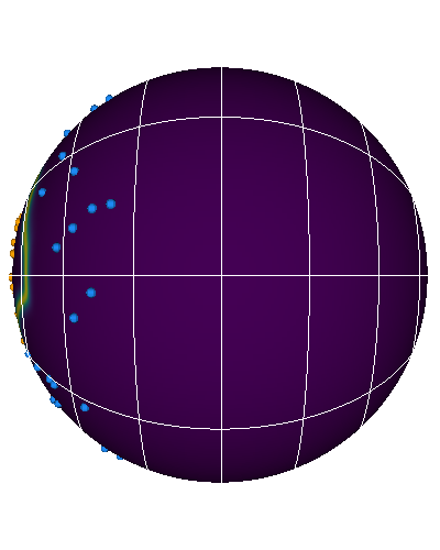
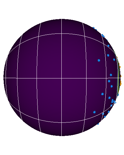
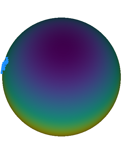
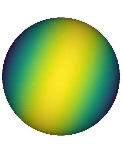
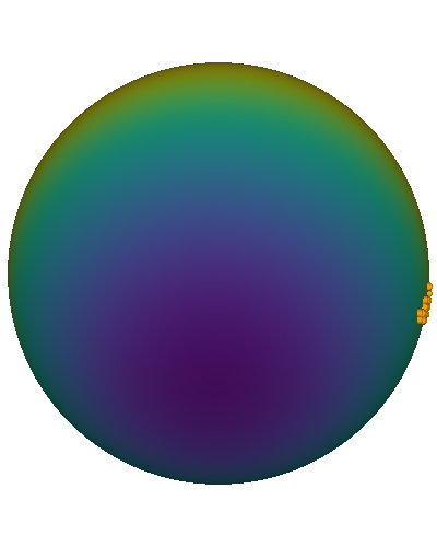
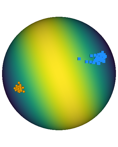
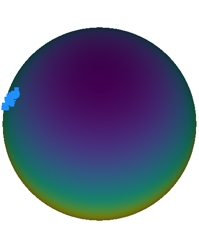
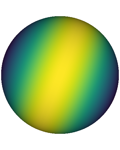
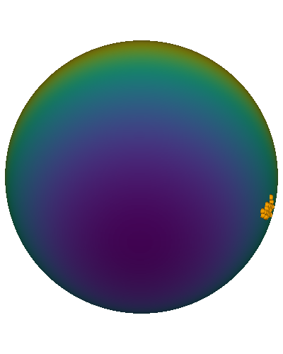
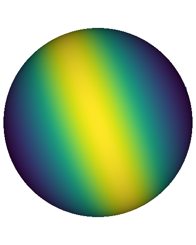
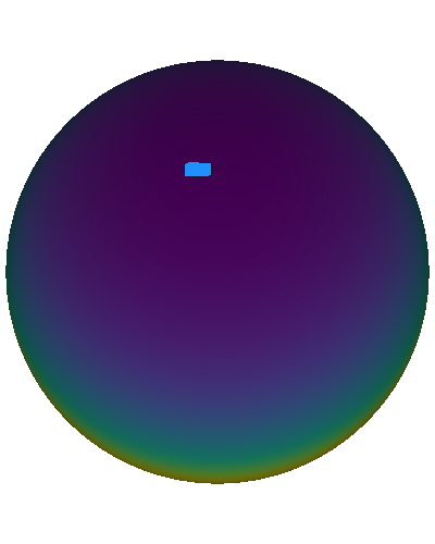
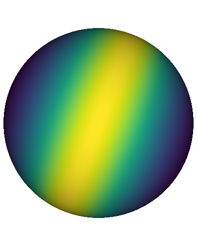
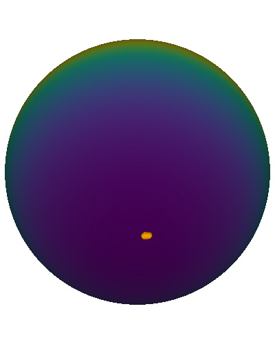
Figure 3 displays the energy landscape of Eb(𝝃;𝑿,𝑶)subscriptE𝑏𝝃𝑿𝑶\mathrm{E}_{b}(\bm{\xi};\bm{X},\bm{O}) using exemplary data on a 3-dimensional sphere. EbsubscriptE𝑏\mathrm{E}_{b} is maximal at the decision boundary between ID and AUX data and decreases with increasing distance from the decision boundary in both directions.

As we show in our theoretical discussion in Appendix D, when modeling the class-conditional densities of the ID and AUX data set as mixtures of Gaussian distributions

p(𝝃|ID)𝑝conditional𝝃ID\displaystyle p(\ \bm{\xi}\ |\ \text{ID}\ ) =1Ni=1N𝒩(𝝃;𝒙i,β1𝑰),absent1𝑁superscriptsubscript𝑖1𝑁𝒩𝝃subscript𝒙𝑖superscript𝛽1𝑰\displaystyle=\frac{1}{N}\sum_{i=1}^{N}\mathcal{N}(\bm{\xi};\bm{x}_{i},\beta^{-1}\bm{I}), (7)
p(𝝃|AUX)𝑝conditional𝝃AUX\displaystyle p(\ \bm{\xi}\ |\ \text{AUX}\ ) =1Ni=1N𝒩(𝝃;𝒐i,β1𝑰),absent1𝑁superscriptsubscript𝑖1𝑁𝒩𝝃subscript𝒐𝑖superscript𝛽1𝑰\displaystyle=\frac{1}{N}\sum_{i=1}^{N}\mathcal{N}(\bm{\xi};\bm{o}_{i},\beta^{-1}\bm{I}), (8)

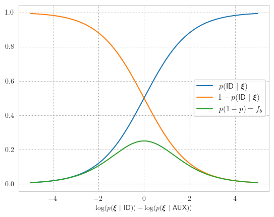
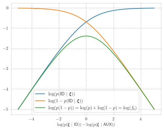
with equal class priors p(ID)=p(AUX)=1/2𝑝ID𝑝AUX12p(\text{ID})=p(\text{AUX})=1/2 and normalized patterns 𝒙i=1normsubscript𝒙𝑖1||\bm{x}_{i}||=1 and 𝒐i=1normsubscript𝒐𝑖1||\bm{o}_{i}||=1, we obtain Eb(𝝃;𝑿,𝑶)=Cβ1log(p(ID|𝝃)p(AUX|𝝃))superscript𝐶subscriptE𝑏𝝃𝑿𝑶superscript𝛽1𝑝conditionalID𝝃𝑝conditionalAUX𝝃\mathrm{E}_{b}(\bm{\xi};\bm{X},\bm{O})\stackrel{{\scriptstyle C}}{{=}}\beta^{-1}\log(p(\ \text{ID}\ |\ \bm{\xi}\ )\cdot p(\ \text{AUX}\ |\ \bm{\xi}\ )), where =Csuperscript𝐶\stackrel{{\scriptstyle C}}{{=}} denotes equality up to an irrelevant additive constant. The exponential of EbsubscriptE𝑏\mathrm{E}_{b} is the variance of a Bernoulli random variable with the outcomes {ID,AUX}IDAUX\{\text{ID},\text{AUX}\} conditioned on 𝝃𝝃\bm{\xi}. Thus, according to EbsubscriptE𝑏\mathrm{E}_{b}, the weak learners are situated at exactly those locations in dsuperscript𝑑\mathbb{R}^{d} where the variance of the model’s decision between the ID and AUX classes is high.

Given a set of query values (𝝃1,𝝃2,,𝝃n)subscript𝝃1subscript𝝃2subscript𝝃𝑛(\bm{\xi}_{1},\bm{\xi}_{2},\dots,\bm{\xi}_{n}) assembled in a query matrix 𝚵d×n𝚵superscript𝑑𝑛\bm{\Xi}\in\mathbb{R}^{d\times n}, we denote a vector of energies 𝒆n𝒆superscript𝑛\bm{e}\in\mathbb{R}^{n} with ei=Eb(𝝃i;𝑿,𝑶)subscript𝑒𝑖subscriptE𝑏subscript𝝃𝑖𝑿𝑶e_{i}=\mathrm{E}_{b}(\bm{\xi}_{i};\bm{X},\bm{O}) as

𝒆=Eb(𝚵;𝑿,𝑶).𝒆subscriptE𝑏𝚵𝑿𝑶\bm{e}=\mathrm{E}_{b}(\bm{\Xi};\bm{X},\bm{O}). (9)

To calculate the weights 𝒘t+1subscript𝒘𝑡1\bm{w}_{t+1}, we use the memory of AUX patterns as a query matrix 𝚵=𝑶𝚵𝑶\bm{\Xi}=\bm{O} and compute the respective energies EbsubscriptE𝑏\mathrm{E}_{b} of those patterns. The resulting energy vector Eb(𝚵;𝑿,𝑶)subscriptE𝑏𝚵𝑿𝑶\mathrm{E}_{b}(\bm{\Xi};\bm{X},\bm{O}) is then normalized by a softmaxsoftmax\mathrm{softmax}. This computation provides the updated weights:

𝒘t+1=softmax(βEb(𝚵;𝑿,𝑶)).subscript𝒘𝑡1softmax𝛽subscriptE𝑏𝚵𝑿𝑶\bm{w}_{t+1}=\mathrm{softmax}(\beta\mathrm{E}_{b}(\bm{\Xi};\bm{X},\bm{O})). (10)

Appendix G provides theoretical background on how informative samples close to the decision boundary are beneficial for training an OOD detector.

Training the model with MHE.

In this section, we introduce how Hopfield Boosting uses the sampled weak learners to improve the detection of patterns outside the training distribution. We follow the established training method for OE (Hendrycks et al., 2019b; Liu et al., 2020; Ming et al., 2022): Train a classifier on the ID data using the standard cross-entropy loss and add an OOD loss that uses the AUX data set to sharpen the decision boundary between the ID and OOD regions. Formally, this yields a composite loss

=CE+λOOD,subscriptCE𝜆subscriptOOD\mathcal{L}=\mathcal{L}_{\text{CE}}+\lambda\mathcal{L}_{\text{OOD}}, (11)

where λ𝜆\lambda is a hyperparamter indicating the relative importance of OODsubscriptOOD\mathcal{L}_{\text{OOD}}. Hopfield Boosting explicitly minimizes EbsubscriptE𝑏\mathrm{E}_{b} (which is also the energy function Hopfield Boosting uses to sample weak learners). Given the weight vector 𝒘tsubscript𝒘𝑡\bm{w}_{t}, and the data sets 𝑿𝒟superscript𝑿𝒟\bm{X}^{\mathcal{D}} and 𝑶𝒟superscript𝑶𝒟\bm{O}^{\mathcal{D}}, we obtain a mini-batch 𝑿s𝒟subscriptsuperscript𝑿𝒟𝑠\bm{X}^{\mathcal{D}}_{s} containing N samples from 𝑿𝒟superscript𝑿𝒟\bm{X}^{\mathcal{D}} by uniform sampling, and a mini-batch of N weak learners 𝑶s𝒟subscriptsuperscript𝑶𝒟𝑠\bm{O}^{\mathcal{D}}_{s} from 𝑶𝒟superscript𝑶𝒟\bm{O}^{\mathcal{D}} by sampling according to 𝒘tsubscript𝒘𝑡\bm{w}_{t} with replacement. We then feed the respective mini-batches into the neural network ϕbasesubscriptitalic-ϕbase\phi_{\text{base}} to create a latent representation (in our experiments, we always use the representation of the penultimate layer of a ResNet). Our proposed approach then uses two heads:

  1. 1.

    A linear classification head that maps the latent representation to the class logits for CEsubscriptCE\mathcal{L}_{\text{CE}}.

  2. 2.

    A 2-layer MLP ϕprojsubscriptitalic-ϕproj\phi_{\text{proj}} maps the representations from the penultimate layer to the output for OODsubscriptOOD\mathcal{L}_{\text{OOD}}.

Hopfield Boosting computes OODsubscriptOOD\mathcal{L}_{\text{OOD}} on the representations it obtains from ϕ=ϕprojϕbaseitalic-ϕsubscriptitalic-ϕprojsubscriptitalic-ϕbase\phi=\phi_{\text{proj}}\circ\phi_{\text{base}} as follows:

OOD=12N𝝃Eb(𝝃;𝑿s,𝑶s),subscriptOOD12𝑁subscript𝝃subscriptE𝑏𝝃subscript𝑿𝑠subscript𝑶𝑠\displaystyle\mathcal{L}_{\text{OOD}}=\frac{1}{2N}\sum_{\bm{\xi}}\mathrm{E}_{b}(\bm{\xi};\bm{X}_{s},\bm{O}_{s}), (12)

where the memories 𝑿ssubscript𝑿𝑠\bm{X}_{s} and 𝑶ssubscript𝑶𝑠\bm{O}_{s} contain the encodings of the sampled data instances: 𝑿s=ϕ(𝑿s𝒟)subscript𝑿𝑠italic-ϕsubscriptsuperscript𝑿𝒟𝑠\bm{X}_{s}=\phi(\bm{X}^{\mathcal{D}}_{s}) and 𝑶s=ϕ(𝑶s𝒟)subscript𝑶𝑠italic-ϕsubscriptsuperscript𝑶𝒟𝑠\bm{O}_{s}=\phi(\bm{O}^{\mathcal{D}}_{s}). The sum is taken over the observations 𝝃𝝃\bm{\xi}, which are drawn from (𝑿s𝑶s)subscript𝑿𝑠subscript𝑶𝑠(\bm{X}_{s}\mathbin{\|}\bm{O}_{s}). Hopfield Boosting computes OODsubscriptOOD\mathcal{L}_{\text{OOD}} for each mini-batch by first calculating the pairwise similarity matrix between the patterns in the mini-batch, followed by determining the EbsubscriptE𝑏\mathrm{E}_{b} values of the individual observations 𝝃𝝃\bm{\xi}, and, finally a mean reduction. To the best of our knowledge, Hopfield Boosting is the first method that uses Hopfield networks in this way to train a deep neural network. We note that there is a relation between Hopfield Boosting and SVMs with an RBF kernel (see Appendix E.3). However, the optimization procedure of SVMs is in general not differentiable. In contrast, our novel energy function is fully differentiable. This allows us to use it to train neural networks.

Summary.

Algorithm 1 Hopfield Boosting
0:  T𝑇T, N𝑁N, 𝑿𝑿\bm{X}, 𝑶𝑶\bm{O}, 𝒀𝒀\bm{Y}, CEsubscriptCE\mathcal{L}_{\text{CE}}, EbsubscriptE𝑏\mathrm{E}_{b}, β𝛽\beta
  Set all weights w1subscript𝑤1w_{1} to 1/|𝑶|1𝑶1/|\bm{O}|
  for t=1𝑡1t=1 to T𝑇T do
     1. Weight. Get hypothesis 𝑿s𝑶s{ID,AUX}subscript𝑿𝑠subscript𝑶𝑠IDAUX\bm{X}_{s}\mathbin{\|}\bm{O}_{s}\rightarrow\{\text{ID},\text{AUX}\}:
     1.a. Mini-batch sampling 𝑿ssubscript𝑿𝑠\bm{X}_{s} from 𝑿𝑿\bm{X}, and
     1.b. \brlapaccording to the weighting 𝒘tsubscript𝒘𝑡\bm{w}_{t}.Sub-sampling of weak learners 𝑶ssubscript𝑶𝑠\bm{O}_{s} from 𝑶𝑶\bm{O}
     2. \brlapEquation (11) on 𝑿ssubscript𝑿𝑠\bm{X}_{s} and 𝑶ssubscript𝑶𝑠\bm{O}_{s}.Evaluate. Compute composite loss from
     3. Update. Update model for the next iteration:
     3.a. \brlap(backbone, classification head, and MHE).At every step, update the full model
     3.b. \brlap𝑶𝑶\bm{O} with 𝒘t+1=softmax(βEb(𝑶;𝑿,𝑶))subscript𝒘𝑡1softmax𝛽subscriptE𝑏𝑶𝑿𝑶\bm{w}_{t+1}=\mathrm{softmax}(\beta\mathrm{E}_{b}(\bm{O};\bm{X},\bm{O})).At every tN𝑡𝑁t*N step calculate new weights for
  end for

return 𝒘tsubscript𝒘𝑡\bm{w}_{t}

Refer to caption
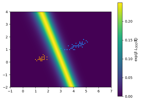
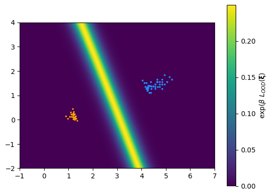
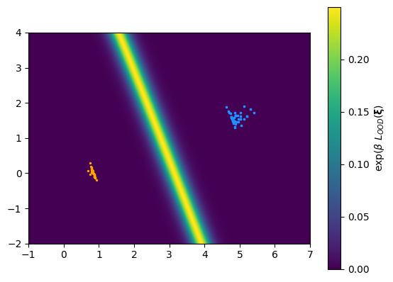
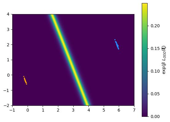
Figure 2: Synthetic example of the adaptive resampling mechanism. Hopfield Boosting forms a strong learner by sampling and combining a set of weak learners close to the decision boundary. The heatmap on the background shows exp(βEb(𝝃,𝑿,𝑶))𝛽subscriptE𝑏𝝃𝑿𝑶\exp(\beta\mathrm{E}_{b}(\bm{\xi},\bm{X},\bm{O})), where β𝛽\beta is 606060. Only the sampled (i.e., highlighted) points serve as memories 𝑿𝑿\bm{X} and 𝑶𝑶\bm{O}.
Refer to caption
(a)
Refer to caption
(b)
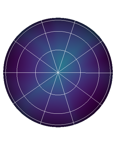
Figure 3: Depiction of the Eb(𝝃;𝑿,𝑶)subscriptE𝑏𝝃𝑿𝑶\mathrm{E}_{b}(\bm{\xi};\bm{X},\bm{O}) energy landscape for separating inliers from AUX data / outliers on a 3D sphere with exemplary inlier (orange) and outlier (blue) points. (a) presents a front view, and (b) rotates the sphere by 90 degrees around the vertical axis. We set β𝛽\beta to 128128128. Appendix C.1 shows the sphere in more orientations.

Algorithm 1 provides an outline of Hopfield Boosting. Each iteration t𝑡t consists of three main steps: 1. weight, 2. evaluate, and 3. update. In the first step, Hopfield Boosting samples a mini-batch from the ID data and weights the AUX data by sampling a mini-batch according to 𝒘tsubscript𝒘𝑡\bm{w}_{t}. Then, Hopfield Boosting evaluates the composite loss on the sampled mini-batch. Lastly, Hopfield Boosting updates the model parameters and, every N𝑁N-th step, also the sampling weights for the AUX data set 𝒘t+1subscript𝒘𝑡1\bm{w}_{t+1}. We created a video111https://youtu.be/H5tGdL-0fok visualizing the learning dynamics of Hopfield Boosting. For more information, we refer to Appendix C.4.

Inference.

At inference time, the OOD score s(𝝃)𝑠𝝃s(\bm{\xi}) is

s(𝝃)=lse(β,𝑿T𝝃)lse(β,𝑶T𝝃).𝑠𝝃lse𝛽superscript𝑿𝑇𝝃lse𝛽superscript𝑶𝑇𝝃\displaystyle s(\bm{\xi})\ =\ \mathrm{lse}(\beta,\bm{X}^{T}\bm{\xi})\ -\ \mathrm{lse}(\beta,\bm{O}^{T}\bm{\xi}). (13)

For computing s(𝝃)𝑠𝝃s(\bm{\xi}), Hopfield Boosting uses the full ID data set and a randomly sampled subset of the AUX data that has identical size. As we show in Appendix F.6, this step entails only a very moderate computational overhead in relation to a complete forward pass (e.g., an overhead of 7.5% for ResNet-18 on an NVIDIA Titan V GPU with 50,000 patterns stored in each of the memories 𝑿𝑿\bm{X} and 𝑶𝑶\bm{O}).

We additionally experimented with using only lse(β,𝑿T𝝃)lse𝛽superscript𝑿𝑇𝝃\mathrm{lse}(\beta,\bm{X}^{T}\bm{\xi}) as a score, which also gives reasonable results. However, the approach in Equation (13) has turned out to be superior. Equation (13) uses information from both ID and AUX samples. This can, for example, be beneficial for handling query patterns 𝝃𝝃\bm{\xi} that are dissimilar from both the memory patterns in 𝑿𝑿\bm{X} as well as from the memory patterns in 𝑶𝑶\bm{O}.

3.4 Comparison of Hopfield Boosting to HE and SHE

Zhang et al. (2023a) propose two post-hoc methods for OOD detection using MHE. They are called “Hopfield Energy” (HE) and “Simplified Hopfield Energy” (SHE). In contrast to Hopfield Boosting, HE and SHE do not make use of AUX data to get a better boundary between ID and OOD data. Rather, their methods evaluate the MHE on ID patterns only to determine whether a sample is ID or OOD. There are also more nuanced differences, for example, Hopfield Boosting uses a single Hopfield network for all ID classes, while HE and SHE employ an individual Hopfield network for each ID class. We provide a more in-depth discussion on the relation to HE and SHE in Appendix E.4.

Table 1: OOD detection performance on CIFAR-10. We compare results from Hopfield Boosting, DOS (Jiang et al., 2024), DOE (Wang et al., 2023b), DivOE (Zhu et al., 2023b), DAL (Wang et al., 2023a), MixOE (Zhang et al., 2023b), POEM (Ming et al., 2022), EBO-OE (Liu et al., 2020), and MSP-OE (Hendrycks et al., 2019b) on ResNet-18. \downarrow indicates “lower is better” and \uparrow “higher is better”. All values in %percent\%. Standard deviations are estimated across five training runs.
OOD Dataset Metric HB (ours) DOS DOE DivOE DAL MixOE POEM EBO-OE MSP-OE
\rowcolorgray!25 FPR95 \downarrow 0.23±0.08superscript0.23plus-or-minus0.08\mathbf{0.23^{\pm 0.08}} 3.09±0.75superscript3.09plus-or-minus0.753.09^{\pm 0.75} 1.97±0.58superscript1.97plus-or-minus0.581.97^{\pm 0.58} 6.21±0.84superscript6.21plus-or-minus0.846.21^{\pm 0.84} 1.25±0.62superscript1.25plus-or-minus0.621.25^{\pm 0.62} 27.54±2.46superscript27.54plus-or-minus2.4627.54^{\pm 2.46} 1.48±0.68superscript1.48plus-or-minus0.681.48^{\pm 0.68} 2.66±0.91superscript2.66plus-or-minus0.912.66^{\pm 0.91} 4.31±1.10superscript4.31plus-or-minus1.104.31^{\pm 1.10}
\rowcolorgray!25 SVHN AUROC \uparrow 99.57±0.06superscript99.57plus-or-minus0.06\mathbf{99.57^{\pm 0.06}} 99.15±0.22superscript99.15plus-or-minus0.2299.15^{\pm 0.22} 99.60±0.13superscript99.60plus-or-minus0.13\mathbf{99.60^{\pm 0.13}} 98.53±0.08superscript98.53plus-or-minus0.0898.53^{\pm 0.08} 99.61±0.15superscript99.61plus-or-minus0.15\mathbf{99.61^{\pm 0.15}} 95.37±0.44superscript95.37plus-or-minus0.4495.37^{\pm 0.44} 99.33±0.15superscript99.33plus-or-minus0.1599.33^{\pm 0.15} 99.15±0.23superscript99.15plus-or-minus0.2399.15^{\pm 0.23} 99.20±0.15superscript99.20plus-or-minus0.1599.20^{\pm 0.15}
\rowcolorwhite FPR95 \downarrow 0.82±0.17superscript0.82plus-or-minus0.170.82^{\pm 0.17} 3.66±0.98superscript3.66plus-or-minus0.983.66^{\pm 0.98} 3.22±0.45superscript3.22plus-or-minus0.453.22^{\pm 0.45} 1.88±0.25superscript1.88plus-or-minus0.251.88^{\pm 0.25} 4.17±0.27superscript4.17plus-or-minus0.274.17^{\pm 0.27} 0.14±0.07superscript0.14plus-or-minus0.07\mathbf{0.14^{\pm 0.07}} 4.02±0.91superscript4.02plus-or-minus0.914.02^{\pm 0.91} 6.82±0.74superscript6.82plus-or-minus0.746.82^{\pm 0.74} 7.02±1.14superscript7.02plus-or-minus1.147.02^{\pm 1.14}
\rowcolorwhite LSUN-Crop AUROC \uparrow 99.40±0.04superscript99.40plus-or-minus0.0499.40^{\pm 0.04} 99.04±0.20superscript99.04plus-or-minus0.2099.04^{\pm 0.20} 99.30±0.12superscript99.30plus-or-minus0.1299.30^{\pm 0.12} 99.50±0.02superscript99.50plus-or-minus0.0299.50^{\pm 0.02} 99.13±0.02superscript99.13plus-or-minus0.0299.13^{\pm 0.02} 99.61±0.11superscript99.61plus-or-minus0.11\mathbf{99.61^{\pm 0.11}} 98.89±0.15superscript98.89plus-or-minus0.1598.89^{\pm 0.15} 98.43±0.10superscript98.43plus-or-minus0.1098.43^{\pm 0.10} 98.83±0.15superscript98.83plus-or-minus0.1598.83^{\pm 0.15}
\rowcolorgray!25 FPR95 \downarrow 0.00±0.00superscript0.00plus-or-minus0.00\mathbf{0.00^{\pm 0.00}} 0.00±0.00superscript0.00plus-or-minus0.000.00^{\pm 0.00} 0.00±0.00superscript0.00plus-or-minus0.00\mathbf{0.00^{\pm 0.00}} 0.00±0.00superscript0.00plus-or-minus0.00\mathbf{0.00^{\pm 0.00}} 0.00±0.00superscript0.00plus-or-minus0.00\mathbf{0.00^{\pm 0.00}} 0.16±0.17superscript0.16plus-or-minus0.170.16^{\pm 0.17} 0.00±0.00superscript0.00plus-or-minus0.00\mathbf{0.00^{\pm 0.00}} 0.00±0.00superscript0.00plus-or-minus0.00\mathbf{0.00^{\pm 0.00}} 0.00±0.00superscript0.00plus-or-minus0.00\mathbf{0.00^{\pm 0.00}}
\rowcolorgray!25 LSUN-Resize AUROC \uparrow 99.98±0.02superscript99.98plus-or-minus0.0299.98^{\pm 0.02} 99.99±0.01superscript99.99plus-or-minus0.0199.99^{\pm 0.01} 100.00±0.00superscript100.00plus-or-minus0.00\mathbf{100.00^{\pm 0.00}} 99.89±0.05superscript99.89plus-or-minus0.0599.89^{\pm 0.05} 99.92±0.05superscript99.92plus-or-minus0.0599.92^{\pm 0.05} 99.89±0.06superscript99.89plus-or-minus0.0699.89^{\pm 0.06} 99.88±0.12superscript99.88plus-or-minus0.1299.88^{\pm 0.12} 99.98±0.02superscript99.98plus-or-minus0.0299.98^{\pm 0.02} 99.96±0.00superscript99.96plus-or-minus0.0099.96^{\pm 0.00}
\rowcolorwhite FPR95 \downarrow 0.16±0.02superscript0.16plus-or-minus0.02\mathbf{0.16^{\pm 0.02}} 1.28±0.20superscript1.28plus-or-minus0.201.28^{\pm 0.20} 2.75±0.57superscript2.75plus-or-minus0.572.75^{\pm 0.57} 1.20±0.11superscript1.20plus-or-minus0.111.20^{\pm 0.11} 0.95±0.13superscript0.95plus-or-minus0.130.95^{\pm 0.13} 4.68±0.22superscript4.68plus-or-minus0.224.68^{\pm 0.22} 0.49±0.04superscript0.49plus-or-minus0.040.49^{\pm 0.04} 1.11±0.17superscript1.11plus-or-minus0.171.11^{\pm 0.17} 2.29±0.16superscript2.29plus-or-minus0.162.29^{\pm 0.16}
\rowcolorwhite Textures AUROC \uparrow 99.84±0.01superscript99.84plus-or-minus0.01\mathbf{99.84^{\pm 0.01}} 99.63±0.04superscript99.63plus-or-minus0.0499.63^{\pm 0.04} 99.35±0.12superscript99.35plus-or-minus0.1299.35^{\pm 0.12} 99.59±0.02superscript99.59plus-or-minus0.0299.59^{\pm 0.02} 99.74±0.01superscript99.74plus-or-minus0.0199.74^{\pm 0.01} 98.91±0.07superscript98.91plus-or-minus0.0798.91^{\pm 0.07} 99.72±0.05superscript99.72plus-or-minus0.0599.72^{\pm 0.05} 99.61±0.02superscript99.61plus-or-minus0.0299.61^{\pm 0.02} 99.57±0.01superscript99.57plus-or-minus0.0199.57^{\pm 0.01}
\rowcolorgray!25 FPR95 \downarrow 0.00±0.00superscript0.00plus-or-minus0.00\mathbf{0.00^{\pm 0.00}} 0.00±0.00superscript0.00plus-or-minus0.00\mathbf{0.00^{\pm 0.00}} 0.00±0.00superscript0.00plus-or-minus0.00\mathbf{0.00^{\pm 0.00}} 0.00±0.00superscript0.00plus-or-minus0.00\mathbf{0.00^{\pm 0.00}} 0.00±0.00superscript0.00plus-or-minus0.00\mathbf{0.00^{\pm 0.00}} 0.17±0.12superscript0.17plus-or-minus0.120.17^{\pm 0.12} 0.00±0.00superscript0.00plus-or-minus0.00\mathbf{0.00^{\pm 0.00}} 0.00±0.00superscript0.00plus-or-minus0.00\mathbf{0.00^{\pm 0.00}} 0.00±0.00superscript0.00plus-or-minus0.00\mathbf{0.00^{\pm 0.00}}
\rowcolorgray!25 iSUN AUROC \uparrow 99.97±0.02superscript99.97plus-or-minus0.0299.97^{\pm 0.02} 99.99±0.01superscript99.99plus-or-minus0.0199.99^{\pm 0.01} 100.00±0.00superscript100.00plus-or-minus0.00\mathbf{100.00^{\pm 0.00}} 99.88±0.05superscript99.88plus-or-minus0.0599.88^{\pm 0.05} 99.93±0.04superscript99.93plus-or-minus0.0499.93^{\pm 0.04} 99.87±0.05superscript99.87plus-or-minus0.0599.87^{\pm 0.05} 99.87±0.12superscript99.87plus-or-minus0.1299.87^{\pm 0.12} 99.98±0.01superscript99.98plus-or-minus0.0199.98^{\pm 0.01} 99.96±0.00superscript99.96plus-or-minus0.0099.96^{\pm 0.00}
\rowcolorwhite FPR95 \downarrow 4.28±0.23superscript4.28plus-or-minus0.23\mathbf{4.28^{\pm 0.23}} 12.26±0.97superscript12.26plus-or-minus0.9712.26^{\pm 0.97} 19.72±2.39superscript19.72plus-or-minus2.3919.72^{\pm 2.39} 13.70±0.50superscript13.70plus-or-minus0.5013.70^{\pm 0.50} 14.22±0.51superscript14.22plus-or-minus0.5114.22^{\pm 0.51} 16.30±1.09superscript16.30plus-or-minus1.0916.30^{\pm 1.09} 7.70±0.68superscript7.70plus-or-minus0.687.70^{\pm 0.68} 11.77±0.68superscript11.77plus-or-minus0.6811.77^{\pm 0.68} 21.42±0.88superscript21.42plus-or-minus0.8821.42^{\pm 0.88}
\rowcolorwhite Places 365 AUROC \uparrow 98.51±0.10superscript98.51plus-or-minus0.10\mathbf{98.51^{\pm 0.10}} 96.63±0.43superscript96.63plus-or-minus0.4396.63^{\pm 0.43} 95.06±0.72superscript95.06plus-or-minus0.7295.06^{\pm 0.72} 96.95±0.09superscript96.95plus-or-minus0.0996.95^{\pm 0.09} 96.77±0.07superscript96.77plus-or-minus0.0796.77^{\pm 0.07} 96.92±0.22superscript96.92plus-or-minus0.2296.92^{\pm 0.22} 97.56±0.26superscript97.56plus-or-minus0.2697.56^{\pm 0.26} 96.39±0.30superscript96.39plus-or-minus0.3096.39^{\pm 0.30} 95.91±0.17superscript95.91plus-or-minus0.1795.91^{\pm 0.17}
\rowcolorwhite FPR95 \downarrow 0.920.92\mathbf{0.92} 3.383.383.38 4.614.614.61 3.833.833.83 3.433.433.43 8.178.178.17 2.282.282.28 3.733.733.73 5.845.845.84
\rowcolorwhite Mean AUROC \uparrow 99.5599.55\mathbf{99.55} 99.0799.0799.07 98.8898.8898.88 99.0699.0699.06 99.1899.1899.18 98.4398.4398.43 99.2199.2199.21 98.9298.9298.92 98.9098.9098.90

Table 2: OOD detection performance on CIFAR-100. We compare results from Hopfield Boosting, DOS (Jiang et al., 2024), DOE (Wang et al., 2023b), DivOE (Zhu et al., 2023b), DAL (Wang et al., 2023a), MixOE (Zhang et al., 2023b), POEM (Ming et al., 2022), EBO-OE (Liu et al., 2020), and MSP-OE (Hendrycks et al., 2019b) on ResNet-18. \downarrow indicates “lower is better” and \uparrow “higher is better”. All values in %percent\%. Standard deviations are estimated across five training runs.
OOD Dataset Metric HB (ours) DOS DOE DivOE DAL MixOE POEM EBO-OE MSP-OE
\rowcolorgray!25 FPR95 \downarrow 13.27±5.46superscript13.27plus-or-minus5.4613.27^{\pm 5.46} 9.84±2.75superscript9.84plus-or-minus2.75\mathbf{9.84^{\pm 2.75}} 19.38±4.60superscript19.38plus-or-minus4.6019.38^{\pm 4.60} 28.77±5.42superscript28.77plus-or-minus5.4228.77^{\pm 5.42} 19.95±2.34superscript19.95plus-or-minus2.3419.95^{\pm 2.34} 41.54±13.16superscript41.54plus-or-minus13.1641.54^{\pm 13.16} 33.59±4.12superscript33.59plus-or-minus4.1233.59^{\pm 4.12} 36.33±2.95superscript36.33plus-or-minus2.9536.33^{\pm 2.95} 19.86±6.90superscript19.86plus-or-minus6.9019.86^{\pm 6.90}
\rowcolorgray!25 SVHN AUROC \uparrow 97.07±0.81superscript97.07plus-or-minus0.8197.07^{\pm 0.81} 97.64±0.39superscript97.64plus-or-minus0.39\mathbf{97.64^{\pm 0.39}} 95.72±1.12superscript95.72plus-or-minus1.1295.72^{\pm 1.12} 94.25±0.98superscript94.25plus-or-minus0.9894.25^{\pm 0.98} 95.69±0.66superscript95.69plus-or-minus0.6695.69^{\pm 0.66} 92.27±2.71superscript92.27plus-or-minus2.7192.27^{\pm 2.71} 94.06±0.51superscript94.06plus-or-minus0.5194.06^{\pm 0.51} 92.93±0.72superscript92.93plus-or-minus0.7292.93^{\pm 0.72} 95.74±1.60superscript95.74plus-or-minus1.6095.74^{\pm 1.60}
\rowcolorwhite FPR95 \downarrow 12.68±2.38superscript12.68plus-or-minus2.38\mathbf{12.68^{\pm 2.38}} 19.40±2.45superscript19.40plus-or-minus2.4519.40^{\pm 2.45} 28.23±2.69superscript28.23plus-or-minus2.6928.23^{\pm 2.69} 35.10±4.23superscript35.10plus-or-minus4.2335.10^{\pm 4.23} 24.24±2.12superscript24.24plus-or-minus2.1224.24^{\pm 2.12} 23.10±7.39superscript23.10plus-or-minus7.3923.10^{\pm 7.39} 15.72±3.46superscript15.72plus-or-minus3.4615.72^{\pm 3.46} 21.06±3.12superscript21.06plus-or-minus3.1221.06^{\pm 3.12} 32.88±1.28superscript32.88plus-or-minus1.2832.88^{\pm 1.28}
\rowcolorwhite LSUN-Crop AUROC \uparrow 96.54±0.65superscript96.54plus-or-minus0.65\mathbf{96.54^{\pm 0.65}} 96.42±0.35superscript96.42plus-or-minus0.35\mathbf{96.42^{\pm 0.35}} 93.79±0.88superscript93.79plus-or-minus0.8893.79^{\pm 0.88} 92.45±0.94superscript92.45plus-or-minus0.9492.45^{\pm 0.94} 95.04±0.43superscript95.04plus-or-minus0.4395.04^{\pm 0.43} 96.11±1.09superscript96.11plus-or-minus1.0996.11^{\pm 1.09} 96.85±0.60superscript96.85plus-or-minus0.60\mathbf{96.85^{\pm 0.60}} 95.79±0.62superscript95.79plus-or-minus0.6295.79^{\pm 0.62} 92.85±0.33superscript92.85plus-or-minus0.3392.85^{\pm 0.33}
\rowcolorgray!25 FPR95 \downarrow 0.00±0.00superscript0.00plus-or-minus0.00\mathbf{0.00^{\pm 0.00}} 0.01±0.00superscript0.01plus-or-minus0.000.01^{\pm 0.00} 0.05±0.04superscript0.05plus-or-minus0.040.05^{\pm 0.04} 0.01±0.00superscript0.01plus-or-minus0.000.01^{\pm 0.00} 0.00±0.00superscript0.00plus-or-minus0.00\mathbf{0.00^{\pm 0.00}} 10.27±10.72superscript10.27plus-or-minus10.7210.27^{\pm 10.72} 0.00±0.00superscript0.00plus-or-minus0.00\mathbf{0.00^{\pm 0.00}} 0.00±0.00superscript0.00plus-or-minus0.00\mathbf{0.00^{\pm 0.00}} 0.03±0.01superscript0.03plus-or-minus0.010.03^{\pm 0.01}
\rowcolorgray!25 LSUN-Resize AUROC \uparrow 99.98±0.01superscript99.98plus-or-minus0.0199.98^{\pm 0.01} 99.96±0.02superscript99.96plus-or-minus0.0299.96^{\pm 0.02} 99.99±0.01superscript99.99plus-or-minus0.0199.99^{\pm 0.01} 99.99±0.00superscript99.99plus-or-minus0.00\mathbf{99.99^{\pm 0.00}} 99.94±0.02superscript99.94plus-or-minus0.0299.94^{\pm 0.02} 97.99±1.92superscript97.99plus-or-minus1.9297.99^{\pm 1.92} 99.57±0.09superscript99.57plus-or-minus0.0999.57^{\pm 0.09} 99.57±0.03superscript99.57plus-or-minus0.0399.57^{\pm 0.03} 99.97±0.00superscript99.97plus-or-minus0.0099.97^{\pm 0.00}
\rowcolorwhite FPR95 \downarrow 2.35±0.13superscript2.35plus-or-minus0.13\mathbf{2.35^{\pm 0.13}} 6.02±0.52superscript6.02plus-or-minus0.526.02^{\pm 0.52} 19.42±1.58superscript19.42plus-or-minus1.5819.42^{\pm 1.58} 11.52±0.49superscript11.52plus-or-minus0.4911.52^{\pm 0.49} 5.22±0.39superscript5.22plus-or-minus0.395.22^{\pm 0.39} 28.99±6.79superscript28.99plus-or-minus6.7928.99^{\pm 6.79} 2.89±0.32superscript2.89plus-or-minus0.322.89^{\pm 0.32} 5.07±0.54superscript5.07plus-or-minus0.545.07^{\pm 0.54} 10.34±0.40superscript10.34plus-or-minus0.4010.34^{\pm 0.40}
\rowcolorwhite Textures AUROC \uparrow 99.22±0.02superscript99.22plus-or-minus0.02\mathbf{99.22^{\pm 0.02}} 98.33±0.11superscript98.33plus-or-minus0.1198.33^{\pm 0.11} 94.93±0.48superscript94.93plus-or-minus0.4894.93^{\pm 0.48} 97.02±0.08superscript97.02plus-or-minus0.0897.02^{\pm 0.08} 98.50±0.16superscript98.50plus-or-minus0.1698.50^{\pm 0.16} 94.24±1.21superscript94.24plus-or-minus1.2194.24^{\pm 1.21} 98.97±0.08superscript98.97plus-or-minus0.0898.97^{\pm 0.08} 98.15±0.16superscript98.15plus-or-minus0.1698.15^{\pm 0.16} 97.42±0.08superscript97.42plus-or-minus0.0897.42^{\pm 0.08}
\rowcolorgray!25 FPR95 \downarrow 0.00±0.00superscript0.00plus-or-minus0.00\mathbf{0.00^{\pm 0.00}} 0.03±0.01superscript0.03plus-or-minus0.010.03^{\pm 0.01} 0.01±0.02superscript0.01plus-or-minus0.020.01^{\pm 0.02} 0.06±0.01superscript0.06plus-or-minus0.010.06^{\pm 0.01} 0.01±0.02superscript0.01plus-or-minus0.020.01^{\pm 0.02} 14.40±13.48superscript14.40plus-or-minus13.4814.40^{\pm 13.48} 0.00±0.00superscript0.00plus-or-minus0.00\mathbf{0.00^{\pm 0.00}} 0.00±0.00superscript0.00plus-or-minus0.00\mathbf{0.00^{\pm 0.00}} 0.08±0.02superscript0.08plus-or-minus0.020.08^{\pm 0.02}
\rowcolorgray!25 iSUN AUROC \uparrow 99.98±0.01superscript99.98plus-or-minus0.0199.98^{\pm 0.01} 99.95±0.02superscript99.95plus-or-minus0.0299.95^{\pm 0.02} 99.99±0.00superscript99.99plus-or-minus0.00\mathbf{99.99^{\pm 0.00}} 99.97±0.00superscript99.97plus-or-minus0.0099.97^{\pm 0.00} 99.93±0.02superscript99.93plus-or-minus0.0299.93^{\pm 0.02} 97.23±2.59superscript97.23plus-or-minus2.5997.23^{\pm 2.59} 99.59±0.09superscript99.59plus-or-minus0.0999.59^{\pm 0.09} 99.57±0.03superscript99.57plus-or-minus0.0399.57^{\pm 0.03} 99.96±0.01superscript99.96plus-or-minus0.0199.96^{\pm 0.01}
\rowcolorwhite FPR95 \downarrow 19.36±1.02superscript19.36plus-or-minus1.0219.36^{\pm 1.02} 32.13±1.55superscript32.13plus-or-minus1.5532.13^{\pm 1.55} 58.68±4.15superscript58.68plus-or-minus4.1558.68^{\pm 4.15} 44.20±0.95superscript44.20plus-or-minus0.9544.20^{\pm 0.95} 33.43±1.11superscript33.43plus-or-minus1.1133.43^{\pm 1.11} 47.01±6.41superscript47.01plus-or-minus6.4147.01^{\pm 6.41} 18.39±0.68superscript18.39plus-or-minus0.68\mathbf{18.39^{\pm 0.68}} 26.68±2.18superscript26.68plus-or-minus2.1826.68^{\pm 2.18} 45.96±0.85superscript45.96plus-or-minus0.8545.96^{\pm 0.85}
\rowcolorwhite Places 365 AUROC \uparrow 95.85±0.37superscript95.85plus-or-minus0.37\mathbf{95.85^{\pm 0.37}} 91.73±0.39superscript91.73plus-or-minus0.3991.73^{\pm 0.39} 83.47±1.55superscript83.47plus-or-minus1.5583.47^{\pm 1.55} 88.28±0.26superscript88.28plus-or-minus0.2688.28^{\pm 0.26} 91.10±0.29superscript91.10plus-or-minus0.2991.10^{\pm 0.29} 89.20±1.86superscript89.20plus-or-minus1.8689.20^{\pm 1.86} 95.03±0.71superscript95.03plus-or-minus0.7195.03^{\pm 0.71} 91.35±0.70superscript91.35plus-or-minus0.7091.35^{\pm 0.70} 87.77±0.15superscript87.77plus-or-minus0.1587.77^{\pm 0.15}
\rowcolorwhite FPR95 \downarrow 7.947.94\mathbf{7.94} 11.2411.2411.24 20.9620.9620.96 19.9419.9419.94 13.8113.8113.81 27.5527.5527.55 11.7611.7611.76 14.8614.8614.86 18.1918.1918.19
\rowcolorwhite Mean AUROC \uparrow 98.1198.11\mathbf{98.11} 97.3497.3497.34 94.6594.6594.65 95.3395.3395.33 96.7096.7096.70 94.5194.5194.51 97.3497.3497.34 96.2396.2396.23 95.6295.6295.62

Table 3: OOD detection performance on ImageNet-1K. We compare results from Hopfield Boosting, DOS (Jiang et al., 2024), DOE (Wang et al., 2023b), DivOE (Zhu et al., 2023b), DAL (Wang et al., 2023a), MixOE (Zhang et al., 2023b), POEM (Ming et al., 2022), EBO-OE (Liu et al., 2020), and MSP-OE (Hendrycks et al., 2019b) on ResNet-50. \downarrow indicates “lower is better” and \uparrow “higher is better”. All values in %percent\%. Standard deviations are estimated across five training runs.
HB (ours) DOS DOE DivOE DAL MixOE POEM EBO-OE MSP-OE
\rowcolorgray!25 FPR95 \downarrow 44.59±1.05superscript44.59plus-or-minus1.0544.59^{\pm 1.05} 40.29±0.93superscript40.29plus-or-minus0.9340.29^{\pm 0.93} 83.83±7.19superscript83.83plus-or-minus7.1983.83^{\pm 7.19} 42.80±0.74superscript42.80plus-or-minus0.7442.80^{\pm 0.74} 43.88±0.66superscript43.88plus-or-minus0.6643.88^{\pm 0.66} 41.05±4.91superscript41.05plus-or-minus4.9141.05^{\pm 4.91} 31.26±0.67superscript31.26plus-or-minus0.6731.26^{\pm 0.67} 29.67±1.26superscript29.67plus-or-minus1.26\mathbf{29.67^{\pm 1.26}} 48.38±0.87superscript48.38plus-or-minus0.8748.38^{\pm 0.87}
\rowcolorgray!25 Textures AUROC \uparrow 88.01±0.57superscript88.01plus-or-minus0.5788.01^{\pm 0.57} 89.88±0.18superscript89.88plus-or-minus0.1889.88^{\pm 0.18} 64.22±9.25superscript64.22plus-or-minus9.2564.22^{\pm 9.25} 88.18±0.06superscript88.18plus-or-minus0.0688.18^{\pm 0.06} 87.39±0.15superscript87.39plus-or-minus0.1587.39^{\pm 0.15} 88.51±1.29superscript88.51plus-or-minus1.2988.51^{\pm 1.29} 92.22±0.14superscript92.22plus-or-minus0.14\mathbf{92.22^{\pm 0.14}} 92.40±0.23superscript92.40plus-or-minus0.23\mathbf{92.40^{\pm 0.23}} 86.25±0.25superscript86.25plus-or-minus0.2586.25^{\pm 0.25}
\rowcolorwhite FPR95 \downarrow 37.37±1.84superscript37.37plus-or-minus1.84\mathbf{37.37^{\pm 1.84}} 59.29±0.96superscript59.29plus-or-minus0.9659.29^{\pm 0.96} 83.73±8.78superscript83.73plus-or-minus8.7883.73^{\pm 8.78} 61.00±0.57superscript61.00plus-or-minus0.5761.00^{\pm 0.57} 65.31±0.61superscript65.31plus-or-minus0.6165.31^{\pm 0.61} 65.14±2.53superscript65.14plus-or-minus2.5365.14^{\pm 2.53} 57.46±0.90superscript57.46plus-or-minus0.9057.46^{\pm 0.90} 57.69±1.61superscript57.69plus-or-minus1.6157.69^{\pm 1.61} 66.01±0.26superscript66.01plus-or-minus0.2666.01^{\pm 0.26}
\rowcolorwhite SUN AUROC \uparrow 91.24±0.52superscript91.24plus-or-minus0.52\mathbf{91.24^{\pm 0.52}} 84.30±0.21superscript84.30plus-or-minus0.2184.30^{\pm 0.21} 72.95±7.94superscript72.95plus-or-minus7.9472.95^{\pm 7.94} 83.64±0.30superscript83.64plus-or-minus0.3083.64^{\pm 0.30} 81.47±0.22superscript81.47plus-or-minus0.2281.47^{\pm 0.22} 82.20±0.72superscript82.20plus-or-minus0.7282.20^{\pm 0.72} 85.38±0.35superscript85.38plus-or-minus0.3585.38^{\pm 0.35} 85.83±0.60superscript85.83plus-or-minus0.6085.83^{\pm 0.60} 81.45±0.20superscript81.45plus-or-minus0.2081.45^{\pm 0.20}
\rowcolorgray!25 FPR95 \downarrow 53.31±2.05superscript53.31plus-or-minus2.05\mathbf{53.31^{\pm 2.05}} 69.72±1.01superscript69.72plus-or-minus1.0169.72^{\pm 1.01} 86.30±6.69superscript86.30plus-or-minus6.6986.30^{\pm 6.69} 71.09±0.60superscript71.09plus-or-minus0.6071.09^{\pm 0.60} 74.46±0.75superscript74.46plus-or-minus0.7574.46^{\pm 0.75} 71.34±1.49superscript71.34plus-or-minus1.4971.34^{\pm 1.49} 68.87±1.05superscript68.87plus-or-minus1.0568.87^{\pm 1.05} 70.03±1.83superscript70.03plus-or-minus1.8370.03^{\pm 1.83} 74.58±0.44superscript74.58plus-or-minus0.4474.58^{\pm 0.44}
\rowcolorgray!25 Places 365 AUROC \uparrow 87.10±0.52superscript87.10plus-or-minus0.52\mathbf{87.10^{\pm 0.52}} 81.62±0.22superscript81.62plus-or-minus0.2281.62^{\pm 0.22} 70.37±7.17superscript70.37plus-or-minus7.1770.37^{\pm 7.17} 80.35±0.33superscript80.35plus-or-minus0.3380.35^{\pm 0.33} 78.72±0.28superscript78.72plus-or-minus0.2878.72^{\pm 0.28} 80.31±0.42superscript80.31plus-or-minus0.4280.31^{\pm 0.42} 81.79±0.40superscript81.79plus-or-minus0.4081.79^{\pm 0.40} 81.35±0.63superscript81.35plus-or-minus0.6381.35^{\pm 0.63} 78.89±0.19superscript78.89plus-or-minus0.1978.89^{\pm 0.19}
\rowcolorwhite FPR95 \downarrow 11.11±0.66superscript11.11plus-or-minus0.66\mathbf{11.11^{\pm 0.66}} 49.55±1.41superscript49.55plus-or-minus1.4149.55^{\pm 1.41} 70.82±13.89superscript70.82plus-or-minus13.8970.82^{\pm 13.89} 30.51±0.42superscript30.51plus-or-minus0.4230.51^{\pm 0.42} 51.92±0.74superscript51.92plus-or-minus0.7451.92^{\pm 0.74} 47.28±1.55superscript47.28plus-or-minus1.5547.28^{\pm 1.55} 45.37±1.79superscript45.37plus-or-minus1.7945.37^{\pm 1.79} 49.02±4.40superscript49.02plus-or-minus4.4049.02^{\pm 4.40} 51.73±1.35superscript51.73plus-or-minus1.3551.73^{\pm 1.35}
\rowcolorwhite iNaturalist AUROC \uparrow 97.65±0.20superscript97.65plus-or-minus0.20\mathbf{97.65^{\pm 0.20}} 90.49±0.38superscript90.49plus-or-minus0.3890.49^{\pm 0.38} 83.82±5.75superscript83.82plus-or-minus5.7583.82^{\pm 5.75} 93.81±0.10superscript93.81plus-or-minus0.1093.81^{\pm 0.10} 88.33±0.21superscript88.33plus-or-minus0.2188.33^{\pm 0.21} 90.19±0.35superscript90.19plus-or-minus0.3590.19^{\pm 0.35} 92.01±0.33superscript92.01plus-or-minus0.3392.01^{\pm 0.33} 91.44±0.79superscript91.44plus-or-minus0.7991.44^{\pm 0.79} 88.51±0.30superscript88.51plus-or-minus0.3088.51^{\pm 0.30}
\rowcolorwhite FPR95 \downarrow 36.6036.60\mathbf{36.60} 54.7154.7154.71 81.1781.1781.17 51.3551.3551.35 58.9058.9058.90 56.2056.2056.20 50.7450.7450.74 51.6051.6051.60 60.1760.1760.17
\rowcolorwhite Mean AUROC \uparrow 91.0091.00\mathbf{91.00} 86.5786.5786.57 72.8472.8472.84 86.4986.4986.49 83.9883.9883.98 85.3085.3085.30 87.8587.8587.85 87.7587.7587.75 83.7883.7883.78
Table 4: OOD detection performance on CIFAR-10. We compare Hopfield Boosting trained with weighted sampling and with random sampling on ResNet-18. \downarrow indicates “lower is better” and \uparrow indicates “higher is better”. All values in %percent\%. Standard deviations are estimated across five training runs.
Weighted Sampling Random Sampling
OOD Dataset FPR95 \downarrow AUROC \uparrow FPR95 \downarrow AUROC \uparrow
\rowcolorgray!25 SVHN 0.23±0.08superscript0.23plus-or-minus0.08\mathbf{0.23^{\pm 0.08}} 99.57±0.06superscript99.57plus-or-minus0.06\mathbf{99.57^{\pm 0.06}} 0.70±0.13superscript0.70plus-or-minus0.130.70^{\pm 0.13} 99.55±0.08superscript99.55plus-or-minus0.08\mathbf{99.55^{\pm 0.08}}
LSUN-Crop 0.82±0.20superscript0.82plus-or-minus0.20\mathbf{0.82^{\pm 0.20}} 99.40±0.05superscript99.40plus-or-minus0.05\mathbf{99.40^{\pm 0.05}} 1.58±0.31superscript1.58plus-or-minus0.311.58^{\pm 0.31} 99.24±0.10superscript99.24plus-or-minus0.1099.24^{\pm 0.10}
\rowcolorgray!25 LSUN-Resize 0.00±0.00superscript0.00plus-or-minus0.00\mathbf{0.00^{\pm 0.00}} 99.98±0.02superscript99.98plus-or-minus0.02\mathbf{99.98^{\pm 0.02}} 0.00±0.00superscript0.00plus-or-minus0.00\mathbf{0.00^{\pm 0.00}} 99.98±0.01superscript99.98plus-or-minus0.01\mathbf{99.98^{\pm 0.01}}
Textures 0.16±0.02superscript0.16plus-or-minus0.02\mathbf{0.16^{\pm 0.02}} 99.85±0.01superscript99.85plus-or-minus0.01\mathbf{99.85^{\pm 0.01}} 0.26±0.06superscript0.26plus-or-minus0.060.26^{\pm 0.06} 99.81±0.02superscript99.81plus-or-minus0.0299.81^{\pm 0.02}
\rowcolorgray!25 iSUN 0.00±0.00superscript0.00plus-or-minus0.00\mathbf{0.00^{\pm 0.00}} 99.97±0.02superscript99.97plus-or-minus0.0299.97^{\pm 0.02} 0.00±0.00superscript0.00plus-or-minus0.00\mathbf{0.00^{\pm 0.00}} 99.99±0.00superscript99.99plus-or-minus0.00\mathbf{99.99^{\pm 0.00}}
Places 365 4.28±0.26superscript4.28plus-or-minus0.26\mathbf{4.28^{\pm 0.26}} 98.51±0.11superscript98.51plus-or-minus0.11\mathbf{98.51^{\pm 0.11}} 6.20±0.21superscript6.20plus-or-minus0.216.20^{\pm 0.21} 97.68±0.21superscript97.68plus-or-minus0.2197.68^{\pm 0.21}
Mean 0.920.92\mathbf{0.92} 99.5599.55\mathbf{99.55} 1.461.461.46 99.3899.3899.38

4 Toy Examples

This section presents two toy examples illustrating the main intuitions behind Hopfield Boosting. For the sake of clarity, none of them considers the inlier classification task that would induce secondary processes, which would obscure the explanations. Formally, this means that we do not consider the first term on the right-hand side of Equation (11). For further toy examples, we refer to Appendix C.

The first example demonstrates how the weighting step in Hopfield Boosting allows good estimations of the decision boundary, even if Hopfield Boosting only samples a small number of weak learners (Figure 2). This is advantageous because the AUX data set contains a large number of data instances that are uninformative for the OOD detection task. For small, low dimensional data, one can always use all the data to compute EbsubscriptE𝑏\mathrm{E}_{b} (Figure 2, a). For large problems (like in Ming et al., 2022), this strategy is difficult, and the naive solution of uniformly sampling N data points would also not work. This will yield many uninformative points (Figure 2, b). When using Hopfield Boosting and sampling N weak learners according to 𝒘tsubscript𝒘𝑡\bm{w}_{t}, the result better approximates the decision boundary of the full data (Figure 2, c).

The second example depicts how inliers and outliers shape the energy surface (Figure 3). We generated patterns so that 𝑿𝑿\bm{X} clusters around a pole and the outliers populate the remaining perimeter of the sphere. This is analogous to the idea that one has access to a large AUX data set, where some data points are more and some less informative for OOD detection (e.g., as conceptualized in Ming et al., 2022).

5 Experiments

5.1 Data & Setup

CIFAR-10 & CIFAR-100.

Our training and evaluation proceeds as follows: We train Hopfield Boosting with ResNet-18 (He et al., 2016) on the CIFAR-10 and CIFAR-100 data sets (Krizhevsky, 2009), respectively. In these settings, we use ImageNet-RC (Chrabaszcz et al., 2017) (a low-resolution version of ImageNet) as the AUX data set. For testing the OOD detection performance, it is crucial to test how well the model can handle inputs from distributions it has never seen during training (i.e., that are different from the ID and the AUX data set): we use the data sets SVHN (Street View House Numbers) (Netzer et al., 2011), Textures (Cimpoi et al., 2014), iSUN (Xu et al., 2015), Places 365 (López-Cifuentes et al., 2020), and two versions of the LSUN data set (Yu et al., 2015) — one where the images are cropped, and one where they are resized to match the resolution of the CIFAR data sets (32x32 pixels). We compute the scores s(𝝃)𝑠𝝃s(\bm{\xi}) as described in Equation (13) and then evaluate the discriminative power of s(𝝃)𝑠𝝃s(\bm{\xi}) between CIFAR and the respective OOD data set using the FPR95 and the AUROC. We use a validation process with different OOD data for model selection. Specifically, we validate the model on MNIST (LeCun et al., 1998), and ImageNet-RC with different pre-processing than in training (resize to 32x32 pixels instead of crop to 32x32 pixels), as well as Gaussian and uniform noise.

ImageNet-1K.

Following Wang et al. (2023b), we evaluate Hopfield Boosting on the large-scale benchmark: We use ImageNet-1K as ID data set and ImageNet-21K (Ridnik et al., 2021) as AUX data set. The OOD test data sets are Textures (Cimpoi et al., 2014), SUN (Xu et al., 2015), Places 365 (López-Cifuentes et al., 2020), and iNaturalist (Van Horn et al., 2018). In this setting, we fine-tune a pre-trained ResNet-50 using Hopfield Boosting.

Baselines.

As mentioned earlier, previous works contain extensive experimental evidence that OE methods offer superior OOD detection performance compared to methods without OE (see e.g., Ming et al., 2022; Wang et al., 2023a). Our experiments in Appendix F.7 confirm this. Therefore, here we focus on a comprehensive comparison of Hopfield Boosting to eight OE methods: MSP-OE (Hendrycks et al., 2019b), EBO-OE (Liu et al., 2020), POEM (Ming et al., 2022), MixOE (Zhang et al., 2023b), DAL (Wang et al., 2023a), DivOE (Zhu et al., 2023b), DOE (Wang et al., 2023b) and DOS (Jiang et al., 2024).

Training setup.

The network trains for 100 epochs (CIFAR-10/100) or 4 epochs (ImageNet-1K), respectively. In each epoch, the model processes the entire ID data set and a selection of AUX samples (sampled according to 𝒘tsubscript𝒘𝑡\bm{w}_{t}). We sample mini-batches of size 128 per data set, resulting in a combined batch size of 256. We evaluate the composite loss from Equation (11) for each resulting mini-batch and update the model accordingly. After an epoch, we update the sample weights, yielding 𝒘t+1subscript𝒘𝑡1\bm{w}_{t+1}. For efficiency reasons, we only compute the weights for 500,000 AUX data instances which we denote as 𝚵𝚵\bm{\Xi}. The weights of the remaining samples are set to 0. During the sample weight update, Hopfield Boosting does not compute gradients or update model parameters. The update of the sample weights 𝒘t+1subscript𝒘𝑡1\bm{w}_{t+1} proceeds as follows: First, we fill the memories 𝑿𝑿\bm{X} and 𝑶𝑶\bm{O} with 50,000 ID samples and 50,000 AUX samples, respectively. Second, we use the obtained 𝑿𝑿\bm{X} and 𝑶𝑶\bm{O} to get the energy Eb(𝚵;𝑿,𝑶)subscriptE𝑏𝚵𝑿𝑶\mathrm{E}_{b}(\bm{\Xi};\bm{X},\bm{O}) for each of the 500,000 AUX samples in 𝚵𝚵\bm{\Xi} and compute 𝒘t+1subscript𝒘𝑡1\bm{w}_{t+1} according to Equation (10). In the following epoch, Hopfield Boosting samples the mini-batches 𝑶s𝒟subscriptsuperscript𝑶𝒟𝑠\bm{O}^{\mathcal{D}}_{s} according to 𝒘t+1subscript𝒘𝑡1\bm{w}_{t+1} with replacement. To allow the storage of even more patterns in the Hopfield memory during the weight update process, one could incorporate a vector similarity engine (e.g., Douze et al., 2024) into the process. This would potentially allow a less noisy estimate of the sample weights. For the sake of simplicity, we did not opt to do this in our implementation of Hopfield Boosting. As we show in section 5.2, Hopfield Boosting achieves state-of-the-art OOD detection results and can scale to large datasets (ImageNet-1K) even without access to a similarity engine.

Hyperparameters.

Like Yang et al. (2022), we use SGD with an initial learning rate of 0.10.10.1 and a weight decay of 51045superscript1045\cdot 10^{-4}. We decrease the learning rate during the training process with a cosine schedule (Loshchilov & Hutter, 2016). We apply these settings to all OOD detection methods that we test. For training Hopfield Boosting, we use a single value for β𝛽\beta throughout the training and evaluation process and for all OOD data sets. We tune the value of β𝛽\beta for each ID data set separately by selecting the value of β𝛽\beta from the set {2,4,8,16,32}2481632\{2,4,8,16,32\} that performs best in the validation process. We select λ𝜆\lambda — the weight for the OOD loss OODsubscriptOOD\mathcal{L}_{\text{OOD}} — from {0.1,0.25,0.5,1.0}0.10.250.51.0\{0.1,0.25,0.5,1.0\}. In our experiments, β=4𝛽4\beta=4 and λ=0.5𝜆0.5\lambda=0.5 yields the best results for CIFAR-10 and CIFAR-100. For ImageNet-1K, we set β=32𝛽32\beta=32 and λ=0.25𝜆0.25\lambda=0.25.

5.2 Results & Discussion

Table 1 summarizes the results for CIFAR-10. Hopfield Boosting achieves equal or better performance compared to the other methods regarding the FPR95 metric for all OOD data sets. It surpasses POEM (the previously best OOD detection approach with OE in our comparison), improving the mean FPR95 metric from 2.28 to 0.92. We observe that all methods tested perform worst on the Places 365 data set. To gain more insights regarding this behavior, we look at the data instances from the Places 365 data set that Hopfield Boosting trained on CIFAR-10 most confidently classifies as in-distribution (i.e., which receive the highest scores s(𝝃)𝑠𝝃s(\bm{\xi})). Visual inspection shows that among those images, a large portion contains objects from semantic classes included in CIFAR-10 (e.g., airplanes, horses, automobiles). We refer to Appendix F.4 for more details.

We also investigate the influence of boosting (Table 4): The experiment shows that the sampling of weak learners contributes considerably to the performance of Hopfield Boosting. Although Hopfield Boosting demonstrates superior performance compared to POEM even without boosting, informative outlier sampling can beat this version on every dataset on the FPR95 metric. As in the other experiments, the results in LSUN-Resize and iSUN are nearly perfect. For additional ablations, we refer to Appendix F.2.

When subjecting Hopfield Boosting to data sets that were designed to show the weakness of OOD detection approaches (Appendix F.5), we identify instances where a substantial number of outliers are wrongly classified as inliers. Testing with EBO-OE yields comparable outcomes, indicating that this phenomenon extends beyond Hopfield Boosting.

For CIFAR-100 (Table 2), Hopfield Boosting also surpasses POEM (the previously best method), improving the mean FPR95 from 11.76 to 7.95. On the SVHN data set, Hopfield Boosting improves the FPR95 metric the most, decreasing it from 33.59 to 13.27.

On ImageNet-1K (Table 3), Hopfield Boosting surpasses all methods in our comparison in terms of both mean FPR95 and mean AUROC. Compared to POEM (the previously best method) Hopfield Boosting improves the mean FPR95 from 50.74 to 36.60. This demonstrates that Hopfield Boosting scales surprisingly well to large-scale settings. This is surprising because, in this setting, we only store 100,000 samples in the Hopfield memory during inference (less than 1% of the samples of the ID and AUX data sets combined).

6 Conclusions & Outlook

We introduce Hopfield Boosting: an approach for OOD detection with OE. Hopfield Boosting uses an energy term to boost a classifier between inlier and outlier data by sampling weak learners that are close to the decision boundary. We illustrate how Hopfield Boosting shapes the energy surface to form a decision boundary. Additionally, we demonstrate how the boosting mechanism creates a sharper decision boundary than with random sampling. We compare Hopfield Boosting to eight modern OOD detection approaches using OE. Overall, Hopfield Boosting shows the best results.

Potential future work comprises: (a) There is a clear opportunity to improve the evaluation procedure for OOD detection. Specifically, it remains unclear how reliably the performance on specific data sets can indicate the general ability to detect OOD inputs. Therefore, we aim to develop an evaluation procedure that addresses these issues, allowing for a more nuanced assessment with a focus on relevant real-world scenarios. This could encompass not only an expansion of data but also the introduction of novel metrics and methodological improvements.

(b) A drawback of OE approaches is their reliance on AUX data. Although OE-based approaches improve the OOD detection capability in general, the selection of the AUX data is crucial, as it determines the characteristics of the decision boundary surrounding the inlier data. In practice, the use of AUX data can be prohibitive in domains where only a few or no outliers at all are available for training the model. Hence, a promising avenue is to explore strategies to more directly control the decision boundary by generating artificial outliers, such as through augmentation techniques.

Acknowledgements

We thank Christian Huber for helpful feedback and fruitful discussions.

The ELLIS Unit Linz, the LIT AI Lab, the Institute for Machine Learning, are supported by the Federal State Upper Austria. We thank the projects AI-MOTION (LIT-2018-6-YOU-212), DeepFlood (LIT-2019-8-YOU-213), Medical Cognitive Computing Center (MC3), INCONTROL-RL (FFG-881064), PRIMAL (FFG-873979), S3AI (FFG-872172), DL for GranularFlow (FFG-871302), EPILEPSIA (FFG-892171), AIRI FG 9-N (FWF-36284, FWF-36235), AI4GreenHeatingGrids(FFG- 899943), INTEGRATE (FFG-892418), ELISE (H2020-ICT-2019-3 ID: 951847), Stars4Waters (HORIZON-CL6-2021-CLIMATE-01-01). We thank Audi.JKU Deep Learning Center, TGW LOGISTICS GROUP GMBH, Silicon Austria Labs (SAL), University SAL Labs initiative, FILL Gesellschaft mbH, Anyline GmbH, Google, ZF Friedrichshafen AG, Robert Bosch GmbH, UCB Biopharma SRL, Merck Healthcare KGaA, Verbund AG, GLS (Univ. Waterloo) Software Competence Center Hagenberg GmbH, TÜV Austria, Frauscher Sensonic, Borealis AG, TRUMPF and the NVIDIA Corporation. This work has been supported by the "University SAL Labs" initiative of Silicon Austria Labs (SAL) and its Austrian partner universities for applied fundamental research for electronic-based systems. We acknowledge EuroHPC Joint Undertaking for awarding us access to Karolina at IT4Innovations, Czech Republic and Leonardo at CINECA, Italy.

References

  • Abbott & Arian (1987) Abbott, L. F. and Arian, Y. Storage capacity of generalized networks. Physical review A, 36(10):5091, 1987.
  • Ahn et al. (2012) Ahn, S., Korattikara, A., and Welling, M. Bayesian posterior sampling via stochastic gradient Fisher scoring. In Proceedings of the 29th International Coference on International Conference on Machine Learning, pp.  1771–1778, Madison, WI, USA, 2012. Omnipress.
  • Auer et al. (2023) Auer, A., Gauch, M., Klotz, D., and Hochreiter, S. Conformal prediction for time series with modern Hopfield networks. arXiv preprint arXiv:2303.12783, 2023.
  • Baldi & Venkatesh (1987) Baldi, P. and Venkatesh, S. S. Number of stable points for spin-glasses and neural networks of higher orders. Physical Review Letters, 58(9):913, 1987.
  • Bishop (1995) Bishop, C. Neural Networks for Pattern Recognition. Oxford University Press, 1995.
  • Bishop (1994) Bishop, C. M. Novelty detection and neural network validation. IEE Proceedings-Vision, Image and Signal processing, 141(4):217–222, 1994.
  • Breiman (1997) Breiman, L. Arcing the edge. Technical report, Citeseer, 1997.
  • Caputo & Niemann (2002) Caputo, B. and Niemann, H. Storage capacity of kernel associative memories. In Artificial Neural Networks—ICANN 2002: International Conference Madrid, Spain, August 28–30, 2002 Proceedings 12, pp.  51–56. Springer, 2002.
  • Chen et al. (1986) Chen, H., Lee, Y., Sun, G., Lee, H., Maxwell, T., and Giles, C. L. High order correlation model for associative memory. In AIP Conference Proceedings, volume 151, pp.  86–99. American Institute of Physics, 1986.
  • Chen et al. (2021) Chen, J., Li, Y., Wu, X., Liang, Y., and Jha, S. Atom: Robustifying out-of-distribution detection using outlier mining. In Machine Learning and Knowledge Discovery in Databases. Research Track: European Conference, ECML PKDD 2021, Bilbao, Spain, September 13–17, 2021, Proceedings, Part III 21, pp.  430–445. Springer, 2021.
  • Chen et al. (2020) Chen, T., Kornblith, S., Norouzi, M., and Hinton, G. A simple framework for contrastive learning of visual representations. In International conference on machine learning, pp.  1597–1607. PMLR, 2020.
  • Chrabaszcz et al. (2017) Chrabaszcz, P., Loshchilov, I., and Hutter, F. A downsampled variant of imagenet as an alternative to the CIFAR datasets. arXiv preprint arXiv:1707.08819, 2017.
  • Cimpoi et al. (2014) Cimpoi, M., Maji, S., Kokkinos, I., Mohamed, S., , and Vedaldi, A. Describing textures in the wild. In Proceedings of the IEEE Conf. on Computer Vision and Pattern Recognition (CVPR), 2014.
  • Cortes & Vapnik (1995) Cortes, C. and Vapnik, V. Support-vector networks. Machine learning, 20(3):273–297, 1995.
  • Demiriz et al. (2002) Demiriz, A., Bennett, K. P., and Shawe-Taylor, J. Linear programming boosting via column generation. Machine Learning, 46:225–254, 2002.
  • Djurisic et al. (2023) Djurisic, A., Bozanic, N., Ashok, A., and Liu, R. Extremely simple activation shaping for out-of-distribution detection. In The Eleventh International Conference on Learning Representations, 2023.
  • Douze et al. (2024) Douze, M., Guzhva, A., Deng, C., Johnson, J., Szilvasy, G., Mazaré, P.-E., Lomeli, M., Hosseini, L., and Jégou, H. The faiss library. 2024.
  • Du et al. (2022) Du, X., Wang, Z., Cai, M., and Li, Y. Vos: Learning what you don’t know by virtual outlier synthesis. arXiv preprint arXiv:2202.01197, 2022.
  • Freund & Schapire (1995) Freund, Y. and Schapire, R. E. A decision-theoretic generalization of on-line learning and an application to boosting. In Computational Learning Theory: Eurocolt ’95, pp.  23–37. Springer-Verlag, 1995.
  • Friedman et al. (2000) Friedman, J., Hastie, T., and Tibshirani, R. Additive logistic regression: a statistical view of boosting (with discussion and a rejoinder by the authors). The annals of statistics, 28(2):337–407, 2000.
  • Fürst et al. (2022) Fürst, A., Rumetshofer, E., Lehner, J., Tran, V. T., Tang, F., Ramsauer, H., Kreil, D., Kopp, M., Klambauer, G., Bitto, A., et al. CLOOB: Modern Hopfield networks with InfoLOOB outperform clip. Advances in neural information processing systems, 35:20450–20468, 2022.
  • Gardner (1987) Gardner, E. Multiconnected neural network models. Journal of Physics A: Mathematical and General, 20(11):3453, 1987.
  • He et al. (2016) He, K., Zhang, X., Ren, S., and Sun, J. Deep residual learning for image recognition. In Proceedings of the IEEE conference on computer vision and pattern recognition, pp.  770–778, 2016.
  • He et al. (2020) He, K., Fan, H., Wu, Y., Xie, S., and Girshick, R. Momentum contrast for unsupervised visual representation learning. In Proceedings of the IEEE/CVF conference on computer vision and pattern recognition, pp.  9729–9738, 2020.
  • Hendrycks & Gimpel (2017) Hendrycks, D. and Gimpel, K. A baseline for detecting misclassified and out-of-distribution examples in neural networks. In International Conference on Learning Representations, 2017. URL https://openreview.net/forum?id=Hkg4TI9xl.
  • Hendrycks et al. (2019a) Hendrycks, D., Basart, S., Mazeika, M., Zou, A., Kwon, J., Mostajabi, M., Steinhardt, J., and Song, D. Scaling out-of-distribution detection for real-world settings. arXiv preprint arXiv:1911.11132, 2019a.
  • Hendrycks et al. (2019b) Hendrycks, D., Mazeika, M., and Dietterich, T. Deep anomaly detection with outlier exposure. In International Conference on Learning Representations, 2019b. URL https://openreview.net/forum?id=HyxCxhRcY7.
  • Hendrycks et al. (2019c) Hendrycks, D., Mazeika, M., Kadavath, S., and Song, D. Using self-supervised learning can improve model robustness and uncertainty. Advances in neural information processing systems, 32, 2019c.
  • Hendrycks et al. (2022) Hendrycks, D., Zou, A., Mazeika, M., Tang, L., Li, B., Song, D., and Steinhardt, J. Pixmix: Dreamlike pictures comprehensively improve safety measures. In Proceedings of the IEEE/CVF Conference on Computer Vision and Pattern Recognition, pp.  16783–16792, 2022.
  • Hopfield (1982) Hopfield, J. J. Neural networks and physical systems with emergent collective computational abilities. Proceedings of the National Academy of Sciences, 79(8):2554–2558, 1982.
  • Hopfield (1984) Hopfield, J. J. Neurons with graded response have collective computational properties like those of two-state neurons. Proceedings of the National Academy of Sciences, 81(10):3088–3092, 1984. doi: 10.1073/pnas.81.10.3088.
  • Horn & Usher (1988) Horn, D. and Usher, M. Capacities of multiconnected memory models. Journal de Physique, 49(3):389–395, 1988.
  • Huang et al. (2021) Huang, R., Geng, A., and Li, Y. On the importance of gradients for detecting distributional shifts in the wild. Advances in Neural Information Processing Systems, 34:677–689, 2021.
  • Jiang et al. (2024) Jiang, W., Cheng, H., Chen, M., Wang, C., and Wei, H. DOS: Diverse outlier sampling for out-of-distribution detection. In The Twelfth International Conference on Learning Representations, 2024. URL https://openreview.net/forum?id=iriEqxFB4y.
  • Krizhevsky (2009) Krizhevsky, A. Learning multiple layers of features from tiny images. Master’s thesis, Deptartment of Computer Science, University of Toronto, 2009.
  • Krotov & Hopfield (2016) Krotov, D. and Hopfield, J. J. Dense associative memory for pattern recognition. In Lee, D. D., Sugiyama, M., Luxburg, U. V., Guyon, I., and Garnett, R. (eds.), Advances in Neural Information Processing Systems, pp.  1172–1180. Curran Associates, Inc., 2016.
  • LeCun et al. (1998) LeCun, Y., Bottou, L., Bengio, Y., and Haffner, P. Gradient-based learning applied to document recognition. Proceedings of the IEEE, 86(11):2278–2324, 1998.
  • Lee et al. (2018) Lee, K., Lee, K., Lee, H., and Shin, J. A simple unified framework for detecting out-of-distribution samples and adversarial attacks. In Bengio, S., Wallach, H., Larochelle, H., Grauman, K., Cesa-Bianchi, N., and Garnett, R. (eds.), Advances in Neural Information Processing Systems, volume 31. Curran Associates, Inc., 2018. URL https://proceedings.neurips.cc/paper/2018/file/abdeb6f575ac5c6676b747bca8d09cc2-Paper.pdf.
  • Liang et al. (2018) Liang, S., Li, Y., and Srikant, R. Enhancing the reliability of out-of-distribution image detection in neural networks. In International Conference on Learning Representations, 2018. URL https://openreview.net/forum?id=H1VGkIxRZ.
  • Liu et al. (2020) Liu, W., Wang, X., Owens, J., and Li, Y. Energy-based out-of-distribution detection. In Larochelle, H., Ranzato, M., Hadsell, R., Balcan, M., and Lin, H. (eds.), Advances in Neural Information Processing Systems, volume 33, pp.  21464–21475. Curran Associates, Inc., 2020. URL https://proceedings.neurips.cc/paper/2020/file/f5496252609c43eb8a3d147ab9b9c006-Paper.pdf.
  • Liu et al. (2023) Liu, X., Lochman, Y., and Zach, C. Gen: Pushing the limits of softmax-based out-of-distribution detection. In Proceedings of the IEEE/CVF Conference on Computer Vision and Pattern Recognition, pp.  23946–23955, 2023.
  • López-Cifuentes et al. (2020) López-Cifuentes, A., Escudero-Vinolo, M., Bescós, J., and García-Martín, Á. Semantic-aware scene recognition. Pattern Recognition, 102:107256, 2020.
  • Loshchilov & Hutter (2016) Loshchilov, I. and Hutter, F. Sgdr: Stochastic gradient descent with warm restarts. arXiv preprint arXiv:1608.03983, 2016.
  • Lu et al. (2024) Lu, H., Gong, D., Wang, S., Xue, J., Yao, L., and Moore, K. Learning with mixture of prototypes for out-of-distribution detection. In The Twelfth International Conference on Learning Representations, 2024. URL https://openreview.net/forum?id=uNkKaD3MCs.
  • McInnes et al. (2018) McInnes, L., Healy, J., and Melville, J. Umap: Uniform manifold approximation and projection for dimension reduction. arXiv preprint arXiv:1802.03426, 2018.
  • Ming et al. (2022) Ming, Y., Fan, Y., and Li, Y. POEM: Out-of-distribution detection with posterior sampling. In Chaudhuri, K., Jegelka, S., Song, L., Szepesvari, C., Niu, G., and Sabato, S. (eds.), Proceedings of the 39th International Conference on Machine Learning, volume 162 of Proceedings of Machine Learning Research, pp.  15650–15665. PMLR, 17–23 Jul 2022. URL https://proceedings.mlr.press/v162/ming22a.html.
  • Ming et al. (2023) Ming, Y., Sun, Y., Dia, O., and Li, Y. How to exploit hyperspherical embeddings for out-of-distribution detection? In The Eleventh International Conference on Learning Representations, 2023.
  • Moody & Darken (1989) Moody, J. and Darken, C. J. Fast learning in networks of locally-tuned processing units. Neural computation, 1(2):281–294, 1989.
  • Morteza & Li (2022) Morteza, P. and Li, Y. Provable guarantees for understanding out-of-distribution detection. In Proceedings of the AAAI Conference on Artificial Intelligence, volume 36, pp.  7831–7840, 2022.
  • Müller et al. (1997) Müller, K.-R., Smola, A. J., Rätsch, G., Schölkopf, B., Kohlmorgen, J., and Vapnik, V. Predicting time series with support vector machines. In International conference on artificial neural networks, pp.  999–1004. Springer, 1997.
  • Netzer et al. (2011) Netzer, Y., Wang, T., Coates, A., Bissacco, A., Wu, B., and Ng, A. Y. Reading digits in natural images with unsupervised feature learning. 2011.
  • Oord et al. (2018) Oord, A. v. d., Li, Y., and Vinyals, O. Representation learning with contrastive predictive coding. arXiv preprint arXiv:1807.03748, 2018.
  • Paischer et al. (2022) Paischer, F., Adler, T., Patil, V., Bitto-Nemling, A., Holzleitner, M., Lehner, S., Eghbal-Zadeh, H., and Hochreiter, S. History compression via language models in reinforcement learning. In International Conference on Machine Learning, pp.  17156–17185. PMLR, 2022.
  • Park et al. (2023) Park, G. Y., Kim, J., Kim, B., Lee, S. W., and Ye, J. C. Energy-based cross attention for Bayesian context update in text-to-image diffusion models. In Thirty-seventh Conference on Neural Information Processing Systems, 2023.
  • Psaltis & Park (1986) Psaltis, D. and Park, C. H. Nonlinear discriminant functions and associative memories. In AIP conference Proceedings, volume 151, pp.  370–375. American Institute of Physics, 1986.
  • Ramsauer et al. (2021) Ramsauer, H., Schäfl, B., Lehner, J., Seidl, P., Widrich, M., Gruber, L., Holzleitner, M., Pavlović, M., Sandve, G. K., Greiff, V., Kreil, D., Kopp, M., Klambauer, G., Brandstetter, J., and Hochreiter, S. Hopfield networks is all you need. In 9th International Conference on Learning Representations (ICLR), 2021. URL https://openreview.net/forum?id=tL89RnzIiCd.
  • Rätsch et al. (2001) Rätsch, G., Onoda, T., and Müller, K.-R. Soft margins for AdaBoost. Machine learning, 42:287–320, 2001.
  • Ridnik et al. (2021) Ridnik, T., Ben-Baruch, E., Noy, A., and Zelnik-Manor, L. Imagenet-21k pretraining for the masses. In Thirty-fifth Conference on Neural Information Processing Systems Datasets and Benchmarks Track (Round 1), 2021.
  • Roth et al. (2022) Roth, K., Pemula, L., Zepeda, J., Schölkopf, B., Brox, T., and Gehler, P. Towards total recall in industrial anomaly detection. In Proceedings of the IEEE/CVF Conference on Computer Vision and Pattern Recognition, pp.  14318–14328, 2022.
  • Ruff et al. (2021) Ruff, L., Kauffmann, J. R., Vandermeulen, R. A., Montavon, G., Samek, W., Kloft, M., Dietterich, T. G., and Müller, K.-R. A unifying review of deep and shallow anomaly detection. Proceedings of the IEEE, 109(5):756–795, 2021.
  • Saleh & Saleh (2022) Saleh, R. A. and Saleh, A. Statistical properties of the log-cosh loss function used in machine learning. arXiv preprint arXiv:2208.04564, 2022.
  • Sanchez-Fernandez et al. (2022) Sanchez-Fernandez, A., Rumetshofer, E., Hochreiter, S., and Klambauer, G. CLOOME: a new search engine unlocks bioimaging databases for queries with chemical structures. bioRxiv, pp.  2022–11, 2022.
  • Schäfl et al. (2022) Schäfl, B., Gruber, L., Bitto-Nemling, A., and Hochreiter, S. Hopular: Modern Hopfield networks for tabular data. arXiv preprint arXiv:2206.00664, 2022.
  • Sehwag et al. (2021) Sehwag, V., Chiang, M., and Mittal, P. Ssd: A unified framework for self-supervised outlier detection. arXiv preprint arXiv:2103.12051, 2021.
  • smeschke (2018) smeschke. Four Shapes. https://www.kaggle.com/datasets/smeschke/four-shapes/, 2018. URL https://www.kaggle.com/datasets/smeschke/four-shapes/.
  • Sun & Li (2022) Sun, Y. and Li, Y. Dice: Leveraging sparsification for out-of-distribution detection. In European Conference on Computer Vision, pp.  691–708. Springer, 2022.
  • Sun et al. (2021) Sun, Y., Guo, C., and Li, Y. React: Out-of-distribution detection with rectified activations. Advances in Neural Information Processing Systems, 34:144–157, 2021.
  • Sun et al. (2022) Sun, Y., Ming, Y., Zhu, X., and Li, Y. Out-of-distribution detection with deep nearest neighbors. In International Conference on Machine Learning, pp.  20827–20840. PMLR, 2022.
  • Tack et al. (2020) Tack, J., Mo, S., Jeong, J., and Shin, J. Csi: Novelty detection via contrastive learning on distributionally shifted instances. Advances in neural information processing systems, 33:11839–11852, 2020.
  • Tao et al. (2023) Tao, L., Du, X., Zhu, X., and Li, Y. Non-parametric outlier synthesis. arXiv preprint arXiv:2303.02966, 2023.
  • Teh et al. (2016) Teh, Y. W., Thiery, A. H., and Vollmer, S. J. Consistency and fluctuations for stochastic gradient Langevin dynamics. J. Mach. Learn. Res., 17(1):193–225, 2016.
  • Van Horn et al. (2018) Van Horn, G., Mac Aodha, O., Song, Y., Cui, Y., Sun, C., Shepard, A., Adam, H., Perona, P., and Belongie, S. The inaturalist species classification and detection dataset. In Proceedings of the IEEE conference on computer vision and pattern recognition, pp.  8769–8778, 2018.
  • Vaswani et al. (2017) Vaswani, A., Shazeer, N., Parmar, N., Uszkoreit, J., Jones, L., Gomez, A. N., Kaiser, L., and Polosukhin, I. Attention is all you need. In Guyon, I., Luxburg, U. V., Bengio, S., Wallach, H., Fergus, R., Vishwanathan, S., and Garnett, R. (eds.), Advances in Neural Information Processing Systems 30, pp.  5998–6008. Curran Associates, Inc., 2017.
  • Wang et al. (2022) Wang, H., Li, Z., Feng, L., and Zhang, W. Vim: Out-of-distribution with virtual-logit matching. In Proceedings of the IEEE/CVF conference on computer vision and pattern recognition, pp.  4921–4930, 2022.
  • Wang et al. (2023a) Wang, Q., Fang, Z., Zhang, Y., Liu, F., Li, Y., and Han, B. Learning to augment distributions for out-of-distribution detection. In NeurIPS, 2023a. URL https://openreview.net/forum?id=OtU6VvXJue.
  • Wang et al. (2023b) Wang, Q., Ye, J., Liu, F., Dai, Q., Kalander, M., Liu, T., Hao, J., and Han, B. Out-of-distribution detection with implicit outlier transformation. arXiv preprint arXiv:2303.05033, 2023b.
  • Wang & Isola (2020) Wang, T. and Isola, P. Understanding contrastive representation learning through alignment and uniformity on the hypersphere. In International Conference on Machine Learning, pp.  9929–9939. PMLR, 2020.
  • Wei et al. (2022a) Wei, H., Xie, R., Cheng, H., Feng, L., An, B., and Li, Y. Mitigating neural network overconfidence with logit normalization. In International conference on machine learning, pp.  23631–23644. PMLR, 2022a.
  • Wei et al. (2022b) Wei, X.-S., Cui, Q., Yang, L., Wang, P., Liu, L., and Yang, J. Rpc: a large-scale and fine-grained retail product checkout dataset, 2022b. URL https://rpc-dataset.github.io/.
  • Welling & Teh (2011) Welling, M. and Teh, Y. W. Bayesian learning via stochastic gradient Langevin dynamics. In Proceedings of the 28th International Conference on Machine Learning, pp.  681–688, Madison, WI, USA, 2011. Omnipress.
  • Widrich et al. (2020) Widrich, M., Schäfl, B., Pavlović, M., Ramsauer, H., Gruber, L., Holzleitner, M., Brandstetter, J., Sandve, G. K., Greiff, V., Hochreiter, S., and Klambauer, G. Modern Hopfield networks and attention for immune repertoire classification. ArXiv, 2007.13505, 2020.
  • Xu et al. (2024) Xu, K., Chen, R., Franchi, G., and Yao, A. Scaling for training time and post-hoc out-of-distribution detection enhancement. In The Twelfth International Conference on Learning Representations, 2024.
  • Xu et al. (2015) Xu, P., Ehinger, K. A., Zhang, Y., Finkelstein, A., Kulkarni, S. R., and Xiao, J. Turkergaze: Crowdsourcing saliency with webcam based eye tracking. arXiv preprint arXiv:1504.06755, 2015.
  • Xu et al. (2018) Xu, P., Chen, J., Zou, D., and Gu, Q. Global convergence of Langevin dynamics based algorithms for nonconvex optimization. In Bengio, S., Wallach, H., Larochelle, H., Grauman, K., Cesa-Bianchi, N., and Garnett, R. (eds.), Advances in Neural Information Processing Systems, volume 31, pp.  3122–3133. Curran Associates, Inc., 2018.
  • Yang et al. (2022) Yang, J., Wang, P., Zou, D., Zhou, Z., Ding, K., Peng, W., Wang, H., Chen, G., Li, B., Sun, Y., et al. Openood: Benchmarking generalized out-of-distribution detection. Advances in Neural Information Processing Systems, 35:32598–32611, 2022.
  • Yu et al. (2015) Yu, F., Seff, A., Zhang, Y., Song, S., Funkhouser, T., and Xiao, J. LSUN: Construction of a large-scale image dataset using deep learning with humans in the loop. arXiv preprint arXiv:1506.03365, 2015.
  • Yun et al. (2019) Yun, S., Han, D., Oh, S. J., Chun, S., Choe, J., and Yoo, Y. Cutmix: Regularization strategy to train strong classifiers with localizable features. In Proceedings of the IEEE/CVF international conference on computer vision, pp.  6023–6032, 2019.
  • Zhang et al. (2018) Zhang, H., Cisse, M., Dauphin, Y. N., and Lopez-Paz, D. mixup: Beyond empirical risk minimization. In International Conference on Learning Representations, 2018.
  • Zhang et al. (2023a) Zhang, J., Fu, Q., Chen, X., Du, L., Li, Z., Wang, G., Han, S., Zhang, D., et al. Out-of-distribution detection based on in-distribution data patterns memorization with modern Hopfield energy. In The Eleventh International Conference on Learning Representations, 2023a.
  • Zhang et al. (2023b) Zhang, J., Inkawhich, N., Linderman, R., Chen, Y., and Li, H. Mixture outlier exposure: Towards out-of-distribution detection in fine-grained environments. In Proceedings of the IEEE/CVF Winter Conference on Applications of Computer Vision (WACV), pp.  5531–5540, January 2023b.
  • Zhang et al. (2020) Zhang, R., Li, C., Zhang, J., Chen, C., and Wilson, A. G. Cyclical stochastic gradient MCMC for Bayesian deep learning. In International Conference on Learning Representations, 2020.
  • Zheng et al. (2020) Zheng, Y., Zhao, Y., Ren, M., Yan, H., Lu, X., Liu, J., and Li, J. Cartoon face recognition: A benchmark dataset. In Proceedings of the 28th ACM International Conference on Multimedia, pp.  2264–2272, 2020.
  • Zhu et al. (2023a) Zhu, F., Cheng, Z., Zhang, X.-Y., and Liu, C.-L. Openmix: Exploring outlier samples for misclassification detection. In Proceedings of the IEEE/CVF Conference on Computer Vision and Pattern Recognition, pp.  12074–12083, 2023a.
  • Zhu et al. (2023b) Zhu, J., Geng, Y., Yao, J., Liu, T., Niu, G., Sugiyama, M., and Han, B. Diversified outlier exposure for out-of-distribution detection via informative extrapolation. Advances in Neural Information Processing Systems, 36, 2023b.

Appendix A Details on Continuous Modern Hopfield Networks

The following arguments are adopted from Fürst et al. (2022) and Ramsauer et al. (2021). Associative memory networks have been designed to store and retrieve samples. Hopfield networks are energy-based, binary associative memories, which were popularized as artificial neural network architectures in the 1980s (Hopfield, 1982, 1984). Their storage capacity can be considerably increased by polynomial terms in the energy function (Chen et al., 1986; Psaltis & Park, 1986; Baldi & Venkatesh, 1987; Gardner, 1987; Abbott & Arian, 1987; Horn & Usher, 1988; Caputo & Niemann, 2002; Krotov & Hopfield, 2016). In contrast to these binary memory networks, we use continuous associative memory networks with far higher storage capacity. These networks are continuous and differentiable, retrieve with a single update, and have exponential storage capacity (and are therefore scalable, i.e., able to tackle large problems; Ramsauer et al., 2021).

Formally, we denote a set of patterns {𝒙1,,𝒙N}dsubscript𝒙1subscript𝒙𝑁superscript𝑑\{\bm{x}_{1},\ldots,\bm{x}_{N}\}\subset\mathbb{R}^{d} that are stacked as columns to the matrix 𝑿=(𝒙1,,𝒙N)𝑿subscript𝒙1subscript𝒙𝑁\bm{X}=\left(\bm{x}_{1},\ldots,\bm{x}_{N}\right) and a state pattern (query) 𝝃d𝝃superscript𝑑\bm{\xi}\in\mathbb{R}^{d} that represents the current state. The largest norm of a stored pattern is M=maxi𝒙i𝑀subscript𝑖normsubscript𝒙𝑖M=\max_{i}{{\left\|\bm{x}_{i}\right\|}}. Then, the energy EE\mathrm{E} of continuous Modern Hopfield Networks with state 𝝃𝝃\bm{\xi} is defined as (Ramsauer et al., 2021)

E=β1log(i=1Nexp(β𝒙iT𝝃))+12𝝃T𝝃+C,Esuperscript𝛽1superscriptsubscript𝑖1𝑁𝛽superscriptsubscript𝒙𝑖𝑇𝝃12superscript𝝃𝑇𝝃C\mathrm{E}\ =\ -\ \beta^{-1}\ \log\left(\sum_{i=1}^{N}\exp(\beta\bm{x}_{i}^{T}\bm{\xi})\right)+\ \frac{1}{2}\ \bm{\xi}^{T}\bm{\xi}\ +\ \mathrm{C}, (14)

where C=β1logN+12M2Csuperscript𝛽1𝑁12superscript𝑀2\mathrm{C}=\beta^{-1}\log N\ +\ \frac{1}{2}\ M^{2}. For energy EE\mathrm{E} and state 𝝃𝝃\bm{\xi}, Ramsauer et al. (2021) proved that the update rule

𝝃new=𝑿softmax(β𝑿T𝝃)superscript𝝃new𝑿softmax𝛽superscript𝑿𝑇𝝃\bm{\xi}^{\mathrm{new}}\ =\ \bm{X}\ \mathrm{softmax}(\beta\bm{X}^{T}\bm{\xi}) (15)

converges globally to stationary points of the energy EE\mathrm{E} and coincides with the attention mechanisms of Transformers (Vaswani et al., 2017; Ramsauer et al., 2021).

The separation ΔisubscriptΔ𝑖\Delta_{i} of a pattern 𝒙isubscript𝒙𝑖\bm{x}_{i} is its minimal dot product difference to any of the other patterns:

Δi=minj,ji(𝒙iT𝒙i𝒙iT𝒙j).subscriptΔ𝑖subscript𝑗𝑗𝑖superscriptsubscript𝒙𝑖𝑇subscript𝒙𝑖superscriptsubscript𝒙𝑖𝑇subscript𝒙𝑗\Delta_{i}=\min_{j,j\not=i}\left(\bm{x}_{i}^{T}\bm{x}_{i}-\bm{x}_{i}^{T}\bm{x}_{j}\right). (16)

A pattern is well-separated from the data if ΔisubscriptΔ𝑖\Delta_{i} is above a given threshold (specified in Ramsauer et al., 2021). If the patterns 𝒙isubscript𝒙𝑖\bm{x}_{i} are well-separated, the update rule Equation 15 converges to a fixed point close to a stored pattern. If some patterns are similar to one another and, therefore, not well-separated, the update rule converges to a fixed point close to the mean of the similar patterns.

The update rule of a Hopfield network thus identifies sample–sample relations between stored patterns. This enables similarity-based learning methods like nearest neighbor search (see Schäfl et al., 2022), which Hopfield Boosting leverages to detect samples outside the distribution of the training data.

Appendix B Notes on Langevin Sampling

Another method that is appropriate for earlier acquired models is to sample the posterior via the Stochastic Gradient Langevin Dynamics (SGLD) (Welling & Teh, 2011). This method is efficient since it iteratively learns from small mini-batches (Welling & Teh, 2011; Ahn et al., 2012). See basic work on Langevin dynamics (Welling & Teh, 2011; Ahn et al., 2012; Teh et al., 2016; Xu et al., 2018). A cyclical stepsize schedule for SGLD was very promising for uncertainty quantification (Zhang et al., 2020). Larger steps discover new modes, while smaller steps characterize each mode and perform the posterior sampling.

Appendix C Toy Examples

C.1 3D Visualizations of EbsubscriptE𝑏\mathrm{E}_{b} Loss in More Orientations

(a) Out-of-Distribution energy function

(b) Exponentiated Out-of-Distribution energy function
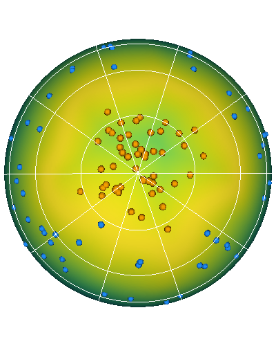
Refer to caption
Refer to caption
Refer to caption
Refer to caption
Refer to caption
Refer to caption
Refer to caption
Refer to caption
Figure 4: Depiction of the energy function Eb(𝝃,𝑿,𝑶)subscriptE𝑏𝝃𝑿𝑶\mathrm{E}_{b}(\bm{\xi},\bm{X},\bm{O}) in Fig. 3 in more orientations. (a) shows Eb(𝝃,𝑿,𝑶)subscriptE𝑏𝝃𝑿𝑶\mathrm{E}_{b}(\bm{\xi},\bm{X},\bm{O}) with exemplary inlier (orange) and outlier (blue) points; and (b) shows exp(βEb(𝝃,𝑿,𝑶))𝛽subscriptE𝑏𝝃𝑿𝑶\exp(\beta\mathrm{E}_{b}(\bm{\xi},\bm{X},\bm{O})). β𝛽\beta was set to 128. Both, (a) and (b), rotate the sphere by 0, 90, 180, and 270 degrees around the vertical axis.

C.2 Dynamics of OODsubscriptOOD\mathcal{L}_{\text{OOD}} on Patterns in Euclidean Space

(a) After 0 steps
Refer to caption
(b) After 25 steps
Refer to caption
(c) After 50 steps
Refer to caption
(d) After 100 steps
Refer to caption
Figure 5: OODsubscriptOOD\mathcal{L}_{\text{OOD}} applied to exemplary data points on euclidean space. Gradient updates are applied to the data points directly. We observe that the variance orthogonal to the decision boundary shrinks while the variance parallel to the decision boundary does not change to this extent. β𝛽\beta is set to 2.

In this example, we applied our out-of-distribution loss OODsubscriptOOD\mathcal{L}_{\text{OOD}} on a simple binary classification problem. As we are working in Euclidean space and not on a sphere, we use a modified version of MHE, which uses the negative squared Euclidean distance instead of the dot-product-similarity. For the formal relation between Equation (17) and MHE, we refer to Appendix E.1:

E(𝝃;𝑿)=β1log(i=1Nexp(β2𝝃𝒙i22))E𝝃𝑿superscript𝛽1superscriptsubscript𝑖1𝑁𝛽2superscriptsubscriptnorm𝝃subscript𝒙𝑖22\displaystyle\mathrm{E}(\bm{\xi};\bm{X})=\ -\ \beta^{-1}\ \log\left(\sum_{i=1}^{N}\exp(-\frac{\beta}{2}\ ||\bm{\xi}-\bm{x}_{i}||_{2}^{2})\right) (17)

Figure 5(a) shows the initial state of the patterns and the decision boundary exp(βEb(𝝃;𝑿,𝑶))𝛽subscript𝐸𝑏𝝃𝑿𝑶\exp(\beta E_{b}(\bm{\xi};\bm{X},\bm{O})). We store the samples of the two classes as stored patterns in 𝑿𝑿\bm{X} and 𝑶𝑶\bm{O}, respectively, and compute OODsubscriptOOD\mathcal{L}_{\text{OOD}} for all samples. We then set the learning rate to 0.1 and perform gradient descent with OODsubscriptOOD\mathcal{L}_{\text{OOD}} on the data points. Figure 5(b) shows that after 25 steps, the distance between the data points and the decision boundary has increased, especially for samples that had previously been close to the decision boundary. After 100 steps, as shown in Figure 5(d), the variability orthogonal to the decision boundary has almost completely vanished, while the variability parallel to the decision boundary is maintained.

C.3 Dynamics of OODsubscriptOOD\mathcal{L}_{\text{OOD}} on Patterns on the Sphere

(a) After 0 steps
(b) After 500 steps
(c) After 2500 steps
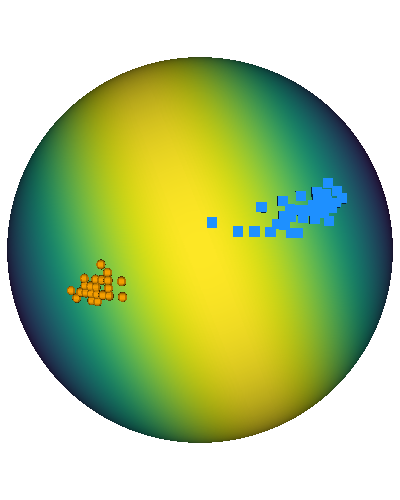
Refer to caption
Refer to caption
Refer to caption
Refer to caption
Refer to caption
Refer to caption
Refer to caption
Refer to caption
Refer to caption
Refer to caption
Refer to caption
Refer to caption
Figure 6: OODsubscriptOOD\mathcal{L}_{\text{OOD}} applied to exemplary data points on a sphere. Gradients are applied to the data points directly. We observe that the geometry of the space forces the patterns to opposing poles of the sphere.

C.4 Learning Dynamics of Hopfield Boosting on Patterns on a Sphere - Video

The example video222https://youtu.be/H5tGdL-0fok

demonstrates the learning dynamics of Hopfield Boosting on a 3-dimensional sphere. We randomly generate ID patterns 𝑿𝑿\bm{X} clustering around one of the sphere’s poles and AUX patterns 𝑶𝑶\bm{O} on the remaining surface of the sphere. We then apply Hopfield Boosting on this data set. First, we sample the weak learners close to the decision boundary for both classes, 𝑿𝑿\bm{X} and 𝑶𝑶\bm{O}. Then, we perform 2000 steps of gradient descent with OODsubscriptOOD\mathcal{L}_{\text{OOD}} on the sampled weak learners. We apply the gradient updates to the patterns directly and do not propagate any gradients to an encoder. Every 50 gradient steps, we re-sample the weak learners. For this example, the initial learning rate is set to 0.020.020.02 and increased after every gradient step by 0.1%percent0.10.1\%.

C.5 Location of Weak Learners near the Decision Boundary
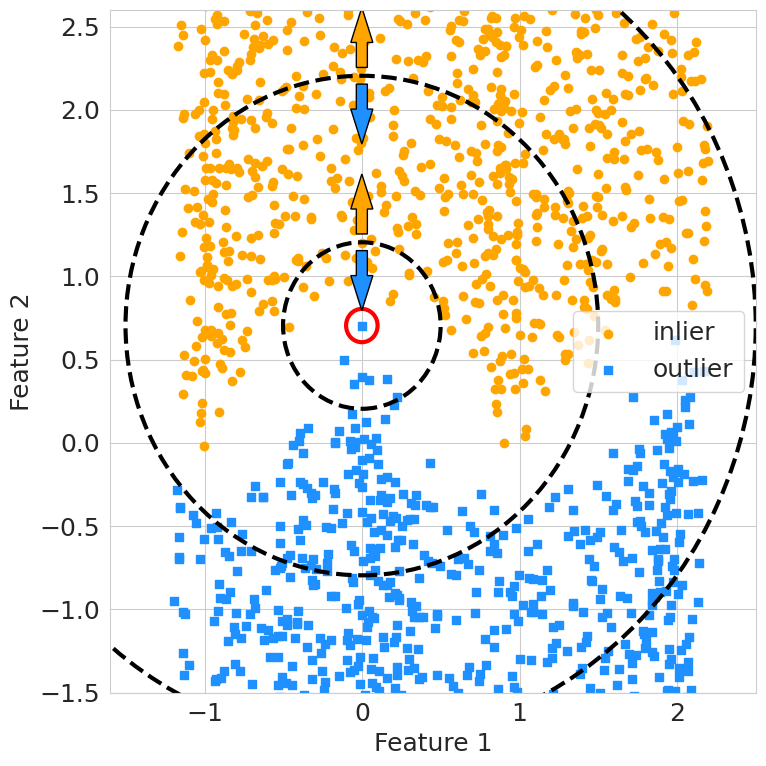
Refer to caption
Figure 7: A prototypical classifier (red circle) that is constructed with a sample close to the decision boundary. Classifiers like this one will only perform slightly better than random guessing (as indicated by the radial decision boundaries) and are, therefore, well-suited for weak learners.

Appendix D Notes on EbsubscriptE𝑏\mathrm{E}_{b}

D.1 Probabilistic Interpretation of EbsubscriptE𝑏\mathrm{E}_{b}

We model the class-conditional densities of the in-distribution data and auxiliary data as mixtures of Gaussians with the patterns as the component means and tied, diagonal covariance matrices with β1superscript𝛽1\beta^{-1} in the main diagonal.

p(𝝃|ID)𝑝conditional𝝃ID\displaystyle p(\ \bm{\xi}\ |\ \text{ID}\ )\ =1Ni=1N𝒩(𝝃;𝒙i,β1𝑰)absent1𝑁superscriptsubscript𝑖1𝑁𝒩𝝃subscript𝒙𝑖superscript𝛽1𝑰\displaystyle=\ \frac{1}{N}\sum_{i=1}^{N}\mathcal{N}\left(\bm{\xi};\bm{x}_{i},\beta^{-1}\bm{I}\right) (18)
p(𝝃|AUX)𝑝conditional𝝃AUX\displaystyle p(\ \bm{\xi}\ |\ \text{AUX}\ )\ =1Mi=1M𝒩(𝝃;𝒐i,β1𝑰)absent1𝑀superscriptsubscript𝑖1𝑀𝒩𝝃subscript𝒐𝑖superscript𝛽1𝑰\displaystyle=\ \frac{1}{M}\sum_{i=1}^{M}\mathcal{N}\left(\bm{\xi};\bm{o}_{i},\beta^{-1}\bm{I}\right) (19)

Further, we assume the distribution p(𝝃)𝑝𝝃p(\bm{\xi}) as a mixture of p(𝝃|ID)𝑝conditional𝝃IDp(\ \bm{\xi}\ |\ \text{ID}\ ) and p(𝝃|AUX)𝑝conditional𝝃AUXp(\ \bm{\xi}\ |\ \text{AUX}\ ) with equal prior probabilities (mixture weights):

p(𝝃)𝑝𝝃\displaystyle p(\bm{\xi})\ =p(ID)p(𝝃|ID)+p(AUX)p(𝝃|AUX)absent𝑝ID𝑝conditional𝝃ID𝑝AUX𝑝conditional𝝃AUX\displaystyle=\ p(\text{ID})\ p(\ \bm{\xi}\ |\ \text{ID}\ )+p(\text{AUX})\ p(\ \bm{\xi}\ |\ \text{AUX}\ ) (20)
=12p(𝝃|ID)+12p(𝝃|AUX)absent12𝑝conditional𝝃ID12𝑝conditional𝝃AUX\displaystyle=\ \frac{1}{2}\ p(\ \bm{\xi}\ |\ \text{ID}\ )\ +\ \frac{1}{2}\ p(\ \bm{\xi}\ |\ \text{AUX}\ ) (21)

The probability of an unknown sample 𝝃𝝃\bm{\xi} being an AUX sample is given by

p(AUX|𝝃)𝑝conditionalAUX𝝃\displaystyle p(\ \text{AUX}\ |\ \bm{\xi}\ )\ =p(𝝃|AUX)p(AUX)p(𝝃)absent𝑝conditional𝝃AUX𝑝AUX𝑝𝝃\displaystyle=\ \frac{p(\ \bm{\xi}\ |\ \text{AUX}\ )\ p(\text{AUX})}{p(\bm{\xi})} (22)
=p(𝝃|AUX)2p(𝝃)absent𝑝conditional𝝃AUX2𝑝𝝃\displaystyle=\frac{p(\ \bm{\xi}\ |\ \text{AUX}\ )}{2\ p(\bm{\xi})} (23)
=p(𝝃|AUX)p(𝝃|AUX)+p(𝝃|ID)absent𝑝conditional𝝃AUX𝑝conditional𝝃AUX𝑝conditional𝝃ID\displaystyle=\frac{p(\ \bm{\xi}\ |\ \text{AUX}\ )}{p(\ \bm{\xi}\ |\ \text{AUX}\ )\ +\ p(\ \bm{\xi}\ |\ \text{ID}\ )} (24)
=11+p(𝝃|ID)p(𝝃|AUX)absent11𝑝conditional𝝃ID𝑝conditional𝝃AUX\displaystyle=\frac{1}{1\ +\ \frac{p(\ \bm{\xi}\ |\ \text{ID}\ )}{p(\ \bm{\xi}\ |\ \text{AUX}\ )}} (25)
=11+exp(log(p(𝝃|ID))log(p(𝝃|AUX)))absent11𝑝conditional𝝃ID𝑝conditional𝝃AUX\displaystyle=\ \frac{1}{1+\exp(\log(p(\ \bm{\xi}\ |\ \text{ID}\ ))-\log(p(\ \bm{\xi}\ |\ \text{AUX}\ )))} (26)

where in line (25) we have used that p(𝝃|AUX)>0𝑝conditional𝝃AUX0p(\ \bm{\xi}\ |\ \text{AUX}\ )>0 for all 𝝃d𝝃superscript𝑑\bm{\xi}\in\mathbb{R}^{d}. The probability of 𝝃𝝃\bm{\xi} being an ID sample is given by

p(ID|𝝃)𝑝conditionalID𝝃\displaystyle p(\ \text{ID}\ |\ \bm{\xi}\ ) =p(𝝃|ID)2p(𝝃)absent𝑝conditional𝝃ID2𝑝𝝃\displaystyle=\frac{p(\ \bm{\xi}\ |\ \text{ID}\ )}{2\ p(\bm{\xi})} (27)
=11+exp(log(p(𝝃|AUX))log(p(𝝃|ID)))absent11𝑝conditional𝝃AUX𝑝conditional𝝃ID\displaystyle=\frac{1}{1+\exp(\log(p(\ \bm{\xi}\ |\ \text{AUX}\ ))-\log(p(\ \bm{\xi}\ |\ \text{ID}\ )))} (28)
=1p(AUX|𝝃)absent1𝑝conditionalAUX𝝃\displaystyle=1-p(\ \text{AUX}\ |\ \bm{\xi}\ ) (29)

Consider the function

fb(𝝃)subscript𝑓𝑏𝝃\displaystyle f_{b}(\bm{\xi})\ =p(AUX|𝝃)p(ID|𝝃)absent𝑝conditionalAUX𝝃𝑝conditionalID𝝃\displaystyle=\ p(\ \text{AUX}\ |\ \bm{\xi})\cdot p(\ \text{ID}\ |\ \bm{\xi}\ ) (30)
=p(𝝃|AUX)p(𝝃|ID)4p(𝝃)2absent𝑝conditional𝝃AUX𝑝conditional𝝃ID4𝑝superscript𝝃2\displaystyle=\frac{p(\ \bm{\xi}\ |\ \text{AUX}\ )\cdot p(\ \bm{\xi}\ |\ \text{ID}\ )}{4p(\bm{\xi})^{2}} (31)

By taking the log\log of Equation (31) we obtain the following. We use =Csuperscript𝐶\ \stackrel{{\scriptstyle C}}{{=}}\ to denote equality up to an additive constant that does not depend on 𝝃𝝃\bm{\xi}.

β1log(fb(𝝃))superscript𝛽1subscript𝑓𝑏𝝃\displaystyle\beta^{-1}\ \log\left(f_{b}(\bm{\xi})\right)\ =C 2β1log(p(𝝃))+β1log(p(𝝃|ID))+β1log(p(𝝃|AUX))superscript𝐶absent2superscript𝛽1𝑝𝝃limit-fromsuperscript𝛽1𝑝conditional𝝃IDsuperscript𝛽1𝑝conditional𝝃AUX\displaystyle\stackrel{{\scriptstyle C}}{{=}}-\ 2\ \beta^{-1}\ \log\left(p(\bm{\xi})\right)\ +\ \beta^{-1}\ \log\left(p(\ \bm{\xi}\ |\ \text{ID}\ )\right)\ +\ \ \beta^{-1}\ \log\left(p(\ \bm{\xi}\ |\ \text{AUX}\ )\right) (32)

Pre-multiplication by β1superscript𝛽1\beta^{-1} is equivalent to a change of base of the log\log. The term β1log(p(𝝃))superscript𝛽1𝑝𝝃-\ \beta^{-1}\ \log(p(\bm{\xi})) is equivalent to the MHE (Ramsauer et al., 2021) (up to an additive constant) when assuming normalized patterns, i.e. 𝒙i2=1subscriptnormsubscript𝒙𝑖21||\bm{x}_{i}||_{2}=1 and 𝒐i2=1subscriptnormsubscript𝒐𝑖21||\bm{o}_{i}||_{2}=1, and an equal number of patterns M=N𝑀𝑁M=N in the two Gaussian mixtures p(𝝃|ID)𝑝conditional𝝃IDp(\ \bm{\xi}\ |\ \text{ID}\ ) and p(𝝃|AUX)𝑝conditional𝝃AUXp(\ \bm{\xi}\ |\ \text{AUX}\ ):

β1log(p(𝝃))superscript𝛽1𝑝𝝃\displaystyle-\ \beta^{-1}\log(p(\bm{\xi})) =β1log(12p(𝝃|ID)+12p(𝝃|AUX))absentsuperscript𝛽112𝑝conditional𝝃ID12𝑝conditional𝝃AUX\displaystyle=-\ \beta^{-1}\log\left(\frac{1}{2}p(\ \bm{\xi}\ |\ \text{ID}\ )\ +\ \frac{1}{2}p(\ \bm{\xi}\ |\ \text{AUX}\ )\right) (33)
=Cβ1log(p(𝝃|ID)+p(𝝃|AUX))superscript𝐶absentsuperscript𝛽1𝑝conditional𝝃ID𝑝conditional𝝃AUX\displaystyle\stackrel{{\scriptstyle C}}{{=}}-\ \beta^{-1}\log\left(p(\ \bm{\xi}\ |\ \text{ID}\ )\ +\ p(\ \bm{\xi}\ |\ \text{AUX}\ )\right) (34)
=β1log(1Ni=1N𝒩(𝝃;𝒙i,β1𝑰)+1Ni=1N𝒩(𝝃;𝒐i,β1𝑰))absentsuperscript𝛽11𝑁superscriptsubscript𝑖1𝑁𝒩𝝃subscript𝒙𝑖superscript𝛽1𝑰1𝑁superscriptsubscript𝑖1𝑁𝒩𝝃subscript𝒐𝑖superscript𝛽1𝑰\displaystyle=-\ \beta^{-1}\log\left(\frac{1}{N}\sum_{i=1}^{N}\mathcal{N}\left(\bm{\xi};\bm{x}_{i},\beta^{-1}\bm{I}\right)\ +\ \frac{1}{N}\sum_{i=1}^{N}\mathcal{N}\left(\bm{\xi};\bm{o}_{i},\beta^{-1}\bm{I}\right)\right) (35)
=Cβ1log(i=1N𝒩(𝝃;𝒙i,β1𝑰)+i=1N𝒩(𝝃;𝒐i,β1𝑰))superscript𝐶absentsuperscript𝛽1superscriptsubscript𝑖1𝑁𝒩𝝃subscript𝒙𝑖superscript𝛽1𝑰superscriptsubscript𝑖1𝑁𝒩𝝃subscript𝒐𝑖superscript𝛽1𝑰\displaystyle\stackrel{{\scriptstyle C}}{{=}}-\ \beta^{-1}\log\left(\sum_{i=1}^{N}\mathcal{N}\left(\bm{\xi};\bm{x}_{i},\beta^{-1}\bm{I}\right)\ +\ \sum_{i=1}^{N}\mathcal{N}\left(\bm{\xi};\bm{o}_{i},\beta^{-1}\bm{I}\right)\right) (36)
=Cβ1log(i=1Nexp(β2𝝃𝒙i22)+i=1Nexp(β2𝝃𝒐i22))superscript𝐶absentsuperscript𝛽1superscriptsubscript𝑖1𝑁𝛽2superscriptsubscriptnorm𝝃subscript𝒙𝑖22superscriptsubscript𝑖1𝑁𝛽2superscriptsubscriptnorm𝝃subscript𝒐𝑖22\displaystyle\stackrel{{\scriptstyle C}}{{=}}-\ \beta^{-1}\log\left(\sum_{i=1}^{N}\exp(-\frac{\beta}{2}||\bm{\xi}-\bm{x}_{i}||_{2}^{2})\ +\ \sum_{i=1}^{N}\exp(-\frac{\beta}{2}||\bm{\xi}-\bm{o}_{i}||_{2}^{2})\right) (37)
=Cβ1log(i=1Nexp(β𝒙iT𝝃β2𝝃T𝝃)+i=1Nexp(β𝒐iT𝝃β2𝝃T𝝃))superscript𝐶absentsuperscript𝛽1superscriptsubscript𝑖1𝑁𝛽superscriptsubscript𝒙𝑖𝑇𝝃𝛽2superscript𝝃𝑇𝝃superscriptsubscript𝑖1𝑁𝛽superscriptsubscript𝒐𝑖𝑇𝝃𝛽2superscript𝝃𝑇𝝃\displaystyle\stackrel{{\scriptstyle C}}{{=}}-\ \beta^{-1}\log\left(\sum_{i=1}^{N}\exp(\beta\bm{x}_{i}^{T}\bm{\xi}-\frac{\beta}{2}\bm{\xi}^{T}\bm{\xi})\ +\ \sum_{i=1}^{N}\exp(\beta\bm{o}_{i}^{T}\bm{\xi}-\frac{\beta}{2}\bm{\xi}^{T}\bm{\xi})\right) (38)
=β1log(i=1Nexp(β𝒙iT𝝃)+i=1Nexp(β𝒐iT𝝃))+12𝝃T𝝃absentsuperscript𝛽1superscriptsubscript𝑖1𝑁𝛽superscriptsubscript𝒙𝑖𝑇𝝃superscriptsubscript𝑖1𝑁𝛽superscriptsubscript𝒐𝑖𝑇𝝃12superscript𝝃𝑇𝝃\displaystyle=-\ \beta^{-1}\log\left(\sum_{i=1}^{N}\exp(\beta\bm{x}_{i}^{T}\bm{\xi})\ +\ \sum_{i=1}^{N}\exp(\beta\bm{o}_{i}^{T}\bm{\xi})\right)\ +\ \frac{1}{2}\ \bm{\xi}^{T}\bm{\xi} (39)
=Clse(β,(𝑿𝑶)T𝝃)+12𝝃T𝝃+β1logN+12M2superscript𝐶absentlse𝛽superscript𝑿𝑶𝑇𝝃12superscript𝝃𝑇𝝃superscript𝛽1𝑁12superscript𝑀2\displaystyle\stackrel{{\scriptstyle C}}{{=}}-\ \mathrm{lse}(\beta,(\bm{X}\mathbin{\|}\bm{O})^{T}\bm{\xi})\ +\ \frac{1}{2}\ \bm{\xi}^{T}\bm{\xi}\ +\beta^{-1}\log N+\frac{1}{2}M^{2} (40)

Analogously, β1log(p(𝝃|ID))superscript𝛽1𝑝conditional𝝃ID\beta^{-1}\ \log(p(\ \bm{\xi}\ |\ \text{ID}\ )) and β1log(p(𝝃|AUX))superscript𝛽1𝑝conditional𝝃AUX\beta^{-1}\ \log(p(\ \bm{\xi}\ |\ \text{AUX}\ )) also yield MHE terms. Therefore, EbsubscriptE𝑏\mathrm{E}_{b} is equivalent to β1log(fb(𝝃))superscript𝛽1subscript𝑓𝑏𝝃\beta^{-1}\log(f_{b}(\bm{\xi})) under the assumption that 𝒙i2=1subscriptnormsubscript𝒙𝑖21||\bm{x}_{i}||_{2}=1 and 𝒐i2=1subscriptnormsubscript𝒐𝑖21||\bm{o}_{i}||_{2}=1 and M=N𝑀𝑁M=N. The 12𝝃T𝝃12superscript𝝃𝑇𝝃\frac{1}{2}\bm{\xi}^{T}\bm{\xi} terms that are contained in the three MHEs cancel out.

β1log(fb(𝝃))=C 2lse(β,(𝑿𝑶)T𝝃)+lse(β,𝑿T𝝃)+lse(β,𝑶T𝝃)=Eb(𝝃;𝑿,𝑶)superscript𝐶superscript𝛽1subscript𝑓𝑏𝝃2lse𝛽superscript𝑿𝑶𝑇𝝃lse𝛽superscript𝑿𝑇𝝃lse𝛽superscript𝑶𝑇𝝃subscriptE𝑏𝝃𝑿𝑶\displaystyle\beta^{-1}\ \log\left(f_{b}(\bm{\xi})\right)\stackrel{{\scriptstyle C}}{{=}}-\ 2\ \mathrm{lse}(\beta,(\bm{X}\mathbin{\|}\bm{O})^{T}\bm{\xi})\ +\ \mathrm{lse}(\beta,\bm{X}^{T}\bm{\xi})\ +\ \mathrm{lse}(\beta,\bm{O}^{T}\bm{\xi})=\mathrm{E}_{b}(\bm{\xi};\bm{X},\bm{O}) (41)

fb(𝝃)subscript𝑓𝑏𝝃f_{b}(\bm{\xi}) can also be interpreted as the variance of a Bernoulli distribution with outcomes ID and AUX:

fb(𝝃)=p(AUX|𝝃)p(ID|𝝃)=p(ID|𝝃)(1p(ID|𝝃))=p(AUX|𝝃)(1p(AUX|𝝃))subscript𝑓𝑏𝝃𝑝conditionalAUX𝝃𝑝conditionalID𝝃𝑝conditionalID𝝃1𝑝conditionalID𝝃𝑝conditionalAUX𝝃1𝑝conditionalAUX𝝃\displaystyle f_{b}(\bm{\xi})=\ p(\ \text{AUX}\ |\ \bm{\xi}\ )\ p(\ \text{ID}\ |\ \bm{\xi}\ )=p(\ \text{ID}\ |\ \bm{\xi}\ )(1-p(\ \text{ID}\ |\ \bm{\xi}\ ))\ =\ p(\ \text{AUX}\ |\ \bm{\xi}\ )(1-p(\ \text{AUX}\ |\ \bm{\xi}\ )) (42)

In other words, minimizing EbsubscriptE𝑏\mathrm{E}_{b} means to drive a Bernoulli-distributed random variable with the outcomes ID and AUX towards minimum variance, i.e., p(ID|𝝃)𝑝conditionalID𝝃p(\ \text{ID}\ |\ \bm{\xi}\ ) is driven towards 111 if p(ID|𝝃)>0.5𝑝conditionalID𝝃0.5p(\ \text{ID}\ |\ \bm{\xi}\ )>0.5 and towards 00 if p(ID|𝝃)<0.5𝑝conditionalID𝝃0.5p(\ \text{ID}\ |\ \bm{\xi}\ )<0.5. Conversely, the same is true for p(AUX|𝝃)𝑝conditionalAUX𝝃p(\ \text{AUX}\ |\ \bm{\xi}\ ).

From Equation (26), under the assumptions that 𝒙i2=1subscriptnormsubscript𝒙𝑖21||\bm{x}_{i}||_{2}=1 and 𝒐i2=1subscriptnormsubscript𝒐𝑖21||\bm{o}_{i}||_{2}=1 and M=N𝑀𝑁M=N, the conditional probability p(AUX|𝝃)𝑝conditionalAUX𝝃p(\ \text{AUX}\ |\ \bm{\xi}\ ) can be computed as follows:

p(AUX|𝝃)𝑝conditionalAUX𝝃\displaystyle p(\ \text{AUX}\ |\ \bm{\xi}\ )\ =σ(log(p(𝝃|AUX))log(p(𝝃|ID)))absent𝜎𝑝conditional𝝃AUX𝑝conditional𝝃ID\displaystyle=\ \sigma(\log(p(\ \bm{\xi}\ |\ \text{AUX}\ ))-\log(p(\ \bm{\xi}\ |\ \text{ID}\ ))) (43)
=σ(β(lse(β,𝑶T𝝃)lse(β,𝑿T𝝃)))absent𝜎𝛽lse𝛽superscript𝑶𝑇𝝃lse𝛽superscript𝑿𝑇𝝃\displaystyle=\ \sigma(\beta\ (\mathrm{lse}(\beta,\bm{O}^{T}\bm{\xi})-\mathrm{lse}(\beta,\bm{X}^{T}\bm{\xi}))) (44)

where σ𝜎\sigma denotes the logistic sigmoid function. Similarly, p(ID|𝝃)𝑝conditionalID𝝃p(\ \text{ID}\ |\ \bm{\xi}\ ) can be computed using

p(ID|𝝃)𝑝conditionalID𝝃\displaystyle p(\ \text{ID}\ |\ \bm{\xi}\ )\ =σ(β(lse(β,𝑿T𝝃)lse(β,𝑶T𝝃)))absent𝜎𝛽lse𝛽superscript𝑿𝑇𝝃lse𝛽superscript𝑶𝑇𝝃\displaystyle=\ \sigma(\beta\ (\mathrm{lse}(\beta,\bm{X}^{T}\bm{\xi})-\mathrm{lse}(\beta,\bm{O}^{T}\bm{\xi}))) (45)
=1p(AUX|𝝃)absent1𝑝conditionalAUX𝝃\displaystyle=1-p(\ \text{AUX}\ |\ \bm{\xi}\ ) (46)

D.2 Alternative Formulations of EbsubscriptE𝑏\mathrm{E}_{b} and fbsubscript𝑓𝑏f_{b}

EbsubscriptE𝑏\mathrm{E}_{b} can be rewritten as follows.

Eb(𝝃;𝑿,𝑶)subscriptE𝑏𝝃𝑿𝑶\displaystyle\mathrm{E}_{b}(\bm{\xi};\bm{X},\bm{O}) = 2lse(β,(𝑿𝑶)T𝝃)+lse(β,𝑿T𝝃)+lse(β,𝑶T𝝃)absent2lse𝛽superscript𝑿𝑶𝑇𝝃lse𝛽superscript𝑿𝑇𝝃lse𝛽superscript𝑶𝑇𝝃\displaystyle=-\ 2\ \mathrm{lse}(\beta,(\bm{X}\mathbin{\|}\bm{O})^{T}\bm{\xi})\ +\ \mathrm{lse}(\beta,\bm{X}^{T}\bm{\xi})\ +\ \mathrm{lse}(\beta,\bm{O}^{T}\bm{\xi}) (47)
= 2β1logcosh(β2(lse(β,𝑿T𝝃)lse(β,𝑶T𝝃))) 2β1log(2)absent2superscript𝛽1𝛽2lse𝛽superscript𝑿𝑇𝝃lse𝛽superscript𝑶𝑇𝝃2superscript𝛽12\displaystyle=\ -\ 2\beta^{-1}\ \log\cosh\left(\frac{\beta}{2}\ (\mathrm{lse}(\beta,\bm{X}^{T}\bm{\xi})\ -\mathrm{lse}(\beta,\bm{O}^{T}\bm{\xi}))\right)\ -\ 2\beta^{-1}\ \log(2) (48)

To prove this, we first show the following:

β1log(exp(βlse(β,𝑿T𝝃))+exp(βlse(β,𝑶T𝝃)))superscript𝛽1𝛽lse𝛽superscript𝑿𝑇𝝃𝛽lse𝛽superscript𝑶𝑇𝝃\displaystyle\ -\ \beta^{-1}\ \log\left(\ \exp(\ \beta\ \mathrm{lse}(\beta,\bm{X}^{T}\bm{\xi})\ )+\exp(\ \beta\ \mathrm{lse}(\beta,\bm{O}^{T}\bm{\xi})\ )\ \right) (49)
=\displaystyle= β1log(exp(ββ1log(i=1Nexp(β𝒙iT𝝃)))+exp(ββ1log(i=1Nexp(β𝒐iT𝝃))))superscript𝛽1𝛽superscript𝛽1superscriptsubscript𝑖1𝑁𝛽superscriptsubscript𝒙𝑖𝑇𝝃𝛽superscript𝛽1superscriptsubscript𝑖1𝑁𝛽superscriptsubscript𝒐𝑖𝑇𝝃\displaystyle\ -\ \beta^{-1}\ \log\left(\ \exp\left(\ \beta\ \beta^{-1}\log\left(\sum_{i=1}^{N}\exp(\beta\bm{x}_{i}^{T}\bm{\xi})\right)\right)+\exp\left(\ \beta\ \beta^{-1}\log\left(\sum_{i=1}^{N}\exp(\beta\bm{o}_{i}^{T}\bm{\xi})\right)\right)\right) (50)
=\displaystyle= β1log(i=1Nexp(β𝒙iT𝝃)+i=1Nexp(β𝒐iT𝝃))superscript𝛽1superscriptsubscript𝑖1𝑁𝛽superscriptsubscript𝒙𝑖𝑇𝝃superscriptsubscript𝑖1𝑁𝛽superscriptsubscript𝒐𝑖𝑇𝝃\displaystyle\ -\ \beta^{-1}\ \log\left(\sum_{i=1}^{N}\exp(\beta\bm{x}_{i}^{T}\bm{\xi})+\sum_{i=1}^{N}\exp(\beta\bm{o}_{i}^{T}\bm{\xi})\right) (51)
=\displaystyle= lse(β,(𝑿𝑶)T𝝃)lse𝛽superscript𝑿𝑶𝑇𝝃\displaystyle\ -\ \mathrm{lse}(\beta,(\bm{X}\mathbin{\|}\bm{O})^{T}\bm{\xi}) (52)

Let E𝑿=lse(β,𝑿T𝝃)subscriptE𝑿lse𝛽superscript𝑿𝑇𝝃\mathrm{E}_{\bm{X}}\ =\ -\mathrm{lse}(\beta,\bm{X}^{T}\bm{\xi}) and E𝑶=lse(β,𝑶T𝝃)subscriptE𝑶lse𝛽superscript𝑶𝑇𝝃\mathrm{E}_{\bm{O}}\ =\ -\mathrm{lse}(\beta,\bm{O}^{T}\bm{\xi}).

Eb(𝝃;𝑿,𝑶)subscriptE𝑏𝝃𝑿𝑶\displaystyle\mathrm{E}_{b}(\bm{\xi};\bm{X},\bm{O})\ = 2lse(β,(𝑿𝑶)T𝝃)+lse(β,𝑿T𝝃)+lse(β,𝑶T𝝃)absent2lse𝛽superscript𝑿𝑶𝑇𝝃lse𝛽superscript𝑿𝑇𝝃lse𝛽superscript𝑶𝑇𝝃\displaystyle=-\ 2\ \mathrm{lse}(\beta,(\bm{X}\mathbin{\|}\bm{O})^{T}\bm{\xi})\ +\ \mathrm{lse}(\beta,\bm{X}^{T}\bm{\xi})\ +\ \mathrm{lse}(\beta,\bm{O}^{T}\bm{\xi}) (53)
= 2β1log(exp(βE𝑿)+exp(βE𝑶))E𝑿E𝑶absent2superscript𝛽1𝛽subscript𝐸𝑿𝛽subscript𝐸𝑶subscript𝐸𝑿subscript𝐸𝑶\displaystyle=\ -\ 2\beta^{-1}\ \log\left(\ \exp(\ -\ \beta\ E_{\bm{X}}\ )+\exp(\ -\ \beta\ E_{\bm{O}}\ )\ \right)\ -\ E_{\bm{X}}\ -\ E_{\bm{O}} (54)
= 2β1log(exp(β2E𝑿)+exp(βE𝑶+β2E𝑿))E𝑶absent2superscript𝛽1𝛽2subscript𝐸𝑿𝛽subscript𝐸𝑶𝛽2subscript𝐸𝑿subscript𝐸𝑶\displaystyle=\ -\ 2\beta^{-1}\ \log\left(\ \exp(\ -\ \frac{\beta}{2}\ E_{\bm{X}}\ )+\exp(\ -\ \beta\ E_{\bm{O}}\ +\frac{\beta}{2}E_{\bm{X}}\ )\ \right)\ -\ E_{\bm{O}} (55)
= 2β1log(exp(β2E𝑿+β2E𝑶)+exp(β2E𝑶+β2E𝑿))absent2superscript𝛽1𝛽2subscript𝐸𝑿𝛽2subscript𝐸𝑶𝛽2subscript𝐸𝑶𝛽2subscript𝐸𝑿\displaystyle=\ -\ 2\beta^{-1}\ \log\left(\ \exp(\ -\ \frac{\beta}{2}\ E_{\bm{X}}+\ \frac{\beta}{2}\ E_{\bm{O}}\ )+\exp(\ -\ \frac{\beta}{2}\ E_{\bm{O}}\ +\frac{\beta}{2}\ E_{\bm{X}}\ )\ \right) (56)
= 2β1logcosh(β2(E𝑿+E𝑶)) 2β1log(2)absent2superscript𝛽1𝛽2subscript𝐸𝑿subscript𝐸𝑶2superscript𝛽12\displaystyle=\ -\ 2\beta^{-1}\ \log\cosh\left(\frac{\beta}{2}(\ -\ E_{\bm{X}}\ +\ E_{\bm{O}})\right)\ -\ 2\beta^{-1}\ \log(2) (57)
= 2β1logcosh(β2(lse(β,𝑿T𝝃)lse(β,𝑶T𝝃))) 2β1log(2)absent2superscript𝛽1𝛽2lse𝛽superscript𝑿𝑇𝝃lse𝛽superscript𝑶𝑇𝝃2superscript𝛽12\displaystyle=\ -\ 2\beta^{-1}\ \log\cosh\left(\frac{\beta}{2}\ (\mathrm{lse}(\beta,\bm{X}^{T}\bm{\xi})\ -\ \mathrm{lse}(\beta,\bm{O}^{T}\bm{\xi}))\right)\ -\ 2\beta^{-1}\ \log(2) (58)
= 2β1logcosh(β2(lse(β,𝑶T𝝃)lse(β,𝑿T𝝃))) 2β1log(2)absent2superscript𝛽1𝛽2lse𝛽superscript𝑶𝑇𝝃lse𝛽superscript𝑿𝑇𝝃2superscript𝛽12\displaystyle=\ -\ 2\beta^{-1}\ \log\cosh\left(\frac{\beta}{2}\ (\mathrm{lse}(\beta,\bm{O}^{T}\bm{\xi})\ -\mathrm{lse}(\beta,\bm{X}^{T}\bm{\xi}))\right)\ -\ 2\beta^{-1}\ \log(2) (59)

By exponentiation of the above result we obtain

fb(𝝃)exp(βEb(𝝃;𝑿,𝑶))proportional-tosubscript𝑓𝑏𝝃𝛽subscriptE𝑏𝝃𝑿𝑶\displaystyle f_{b}(\bm{\xi})\propto\exp(\beta\mathrm{E}_{b}(\bm{\xi};\bm{X},\bm{O}))\ =14cosh2(β2(lse(β,𝑿T𝝃)lse(β,𝑶T𝝃)))absent14superscript2𝛽2lse𝛽superscript𝑿𝑇𝝃lse𝛽superscript𝑶𝑇𝝃\displaystyle=\ \frac{1}{4\cosh^{2}\left(\frac{\beta}{2}\ (\mathrm{lse}(\beta,\bm{X}^{T}\bm{\xi})\ -\ \mathrm{lse}(\beta,\bm{O}^{T}\bm{\xi}))\right)} (60)

The function logcosh(x)𝑥\log\cosh(x) is related to the negative log-likelihood of the hyperbolic secant distribution (see e.g. Saleh & Saleh, 2022). For values of x𝑥x close to 00, logcosh\log\cosh can be approximated by x22superscript𝑥22\frac{x^{2}}{2}, and for values far from 00, the function behaves as |x|log(2)𝑥2|x|-\log(2).

Refer to caption
(a) Probabilities
Refer to caption
(b) Log-probabilities
Figure 8: The product of two logistic sigmoids yields fbsubscript𝑓𝑏f_{b} (a); the sum of two log-sigmoids yields log(fb)subscript𝑓𝑏\log(f_{b}) = EbsubscriptE𝑏\mathrm{E}_{b} (b).

D.3 Derivatives of EbsubscriptE𝑏\mathrm{E}_{b}

In this section, we investigate the derivatives of the energy function EbsubscriptE𝑏\mathrm{E}_{b}. The derivative of the lselse\mathrm{lse} is:

𝒛lse(β,𝒛)=𝒛β1log(i=1Nexp(βzi))=softmax(β𝒛)subscript𝒛lse𝛽𝒛subscript𝒛superscript𝛽1superscriptsubscript𝑖1𝑁𝛽subscript𝑧𝑖softmax𝛽𝒛\displaystyle\nabla_{\bm{z}}\ \mathrm{lse}(\beta,\bm{z})\ =\ \nabla_{\bm{z}}\ \beta^{-1}\ \log\left(\sum_{i=1}^{N}\exp(\beta z_{i})\right)\ =\ \mathrm{softmax}(\beta\ \bm{z}) (61)

Thus, the derivative of the MHE E(𝝃;𝑿)E𝝃𝑿\mathrm{E}(\bm{\xi};\bm{X}) w.r.t. 𝝃𝝃\bm{\xi} is:

𝝃E(𝝃;𝑿)=𝝃(lse(β,𝑿T𝝃)+12𝝃T𝝃+C)=𝑿softmax(β𝑿T𝝃)+𝝃subscript𝝃E𝝃𝑿subscript𝝃lse𝛽superscript𝑿𝑇𝝃12superscript𝝃𝑇𝝃𝐶𝑿softmax𝛽superscript𝑿𝑇𝝃𝝃\displaystyle\nabla_{\bm{\xi}}\ \mathrm{E}(\bm{\xi};\bm{X})\ =\ \nabla_{\bm{\xi}}\ (-\mathrm{lse}(\beta,\bm{X}^{T}\bm{\xi})\ +\ \frac{1}{2}\bm{\xi}^{T}\bm{\xi}\ +\ C)\ =\ -\ \bm{X}\mathrm{softmax}(\beta\bm{X}^{T}\bm{\xi})+\bm{\xi} (62)

The update rule of the MHN

𝝃t+1=𝑿softmax(β𝑿T𝝃t)superscript𝝃𝑡1𝑿softmax𝛽superscript𝑿𝑇superscript𝝃𝑡\displaystyle\bm{\xi}^{t+1}\ =\ \bm{X}\mathrm{softmax}(\beta\bm{X}^{T}\bm{\xi}^{t}) (63)

is derived via the concave-convex procedure. It coincides with the attention mechanisms of Transformers and has been proven to converge globally to stationary points of the energy E(𝝃;𝑿)E𝝃𝑿\mathrm{E}(\bm{\xi};\bm{X}) (Ramsauer et al., 2021). It can also be shown that the update rule emerges when performing gradient descent on E(𝝃;𝑿)E𝝃𝑿\mathrm{E}(\bm{\xi};\bm{X}) with step size η=1𝜂1\eta=1 (Park et al., 2023):

𝝃t+1=𝝃tη𝝃E(𝝃t;𝑿)superscript𝝃𝑡1superscript𝝃𝑡𝜂subscript𝝃Esuperscript𝝃𝑡𝑿\displaystyle\bm{\xi}^{t+1}\ =\ \bm{\xi}^{t}\ -\ \eta\ \nabla_{\bm{\xi}}\mathrm{E}(\bm{\xi}^{t};\bm{X}) (64)
𝝃t+1=𝑿softmax(β𝑿T𝝃t)superscript𝝃𝑡1𝑿softmax𝛽superscript𝑿𝑇superscript𝝃𝑡\displaystyle\bm{\xi}^{t+1}\ =\ \bm{X}\mathrm{softmax}(\beta\bm{X}^{T}\bm{\xi}^{t}) (65)

From Equation (62), we can see that the gradient of Eb(𝝃;𝑿,𝑶)subscriptE𝑏𝝃𝑿𝑶\mathrm{E}_{b}(\bm{\xi};\bm{X},\bm{O}) w.r.t. 𝝃𝝃\bm{\xi} is:

𝝃Eb(𝝃;𝑿,𝑶)subscript𝝃subscriptE𝑏𝝃𝑿𝑶\displaystyle\nabla_{\bm{\xi}}\mathrm{E}_{b}(\bm{\xi};\bm{X},\bm{O})\ =𝝃( 2lse(β,(𝑿𝑶)T𝝃)+lse(β,𝑿T𝝃)+lse(β,𝑶T𝝃))absentsubscript𝝃2lse𝛽superscript𝑿𝑶𝑇𝝃lse𝛽superscript𝑿𝑇𝝃lse𝛽superscript𝑶𝑇𝝃\displaystyle=\ \nabla_{\bm{\xi}}\ (-\ 2\ \mathrm{lse}(\beta,(\bm{X}\mathbin{\|}\bm{O})^{T}\bm{\xi})\ +\ \mathrm{lse}(\beta,\bm{X}^{T}\bm{\xi})\ +\ \mathrm{lse}(\beta,\bm{O}^{T}\bm{\xi})) (66)
= 2(𝑿𝑶)softmax(β(𝑿𝑶)T𝝃)+𝑿softmax(β𝑿T𝝃)+𝑶softmax(β𝑶T𝝃)absent2𝑿𝑶softmax𝛽superscript𝑿𝑶𝑇𝝃𝑿softmax𝛽superscript𝑿𝑇𝝃𝑶softmax𝛽superscript𝑶𝑇𝝃\displaystyle=-\ 2\ (\bm{X}\mathbin{\|}\bm{O})\ \mathrm{softmax}(\beta(\bm{X}\mathbin{\|}\bm{O})^{T}\bm{\xi})\ +\ \bm{X}\mathrm{softmax}(\beta\bm{X}^{T}\bm{\xi})\ +\ \bm{O}\mathrm{softmax}(\beta\bm{O}^{T}\bm{\xi}) (67)

When 𝑿softmax(β𝑿T𝝃)𝑿softmax𝛽superscript𝑿𝑇𝝃\bm{X}\mathrm{softmax}(\beta\bm{X}^{T}\bm{\xi}), 𝑶softmax(β𝑶T𝝃)𝑶softmax𝛽superscript𝑶𝑇𝝃\bm{O}\mathrm{softmax}(\beta\bm{O}^{T}\bm{\xi}), lse(β,𝑿T𝝃)lse𝛽superscript𝑿𝑇𝝃\mathrm{lse}(\beta,\bm{X}^{T}\bm{\xi}) and lse(β,𝑶T𝝃)lse𝛽superscript𝑶𝑇𝝃\mathrm{lse}(\beta,\bm{O}^{T}\bm{\xi}) are available, one can efficiently compute (𝑿𝑶)softmax(β(𝑿𝑶)T𝝃)𝑿𝑶softmax𝛽superscript𝑿𝑶𝑇𝝃(\bm{X}\mathbin{\|}\bm{O})\ \mathrm{softmax}(\beta(\bm{X}\mathbin{\|}\bm{O})^{T}\bm{\xi}) as follows:

(𝑿𝑶)softmax(β(𝑿𝑶)T𝝃)𝑿𝑶softmax𝛽superscript𝑿𝑶𝑇𝝃\displaystyle(\bm{X}\mathbin{\|}\bm{O})\ \mathrm{softmax}(\beta(\bm{X}\mathbin{\|}\bm{O})^{T}\bm{\xi})\ =𝝃lse(β,(𝑿𝑶)T𝝃)absentsubscript𝝃lse𝛽superscript𝑿𝑶𝑇𝝃\displaystyle=\ \nabla_{\bm{\xi}}\ \mathrm{lse}(\beta,(\bm{X}\mathbin{\|}\bm{O})^{T}\bm{\xi}) (68)
=𝝃β1log(exp(βlse(β,𝑿T𝝃))+exp(βlse(β,𝑶T𝝃)))absentsubscript𝝃superscript𝛽1𝛽lse𝛽superscript𝑿𝑇𝝃𝛽lse𝛽superscript𝑶𝑇𝝃\displaystyle=\ \nabla_{\bm{\xi}}\ \beta^{-1}\log\left(\exp(\beta\mathrm{lse}(\beta,\bm{X}^{T}\bm{\xi}))\ +\ \exp(\beta\mathrm{lse}(\beta,\bm{O}^{T}\bm{\xi}))\right) (69)
=(𝑿softmax(β𝑿T𝝃)𝑶softmax(β𝑶T𝝃))softmax(β(lse(β,𝑿T𝝃)lse(β,𝑶T𝝃)))absentmatrix𝑿softmax𝛽superscript𝑿𝑇𝝃𝑶softmax𝛽superscript𝑶𝑇𝝃softmax𝛽matrixlse𝛽superscript𝑿𝑇𝝃lse𝛽superscript𝑶𝑇𝝃\displaystyle=\begin{pmatrix}\bm{X}\mathrm{softmax}(\beta\bm{X}^{T}\bm{\xi})&\bm{O}\mathrm{softmax}(\beta\bm{O}^{T}\bm{\xi})\end{pmatrix}\mathrm{softmax}\left(\beta\begin{pmatrix}\mathrm{lse}(\beta,\bm{X}^{T}\bm{\xi})\\ \mathrm{lse}(\beta,\bm{O}^{T}\bm{\xi})\end{pmatrix}\right) (70)

We can also compute the gradient of Eb(𝝃;𝑿,𝑶)subscriptE𝑏𝝃𝑿𝑶\mathrm{E}_{b}(\bm{\xi};\bm{X},\bm{O}) w.r.t. 𝝃𝝃\bm{\xi} via the logcosh\log\cosh-representation of EbsubscriptE𝑏\mathrm{E}_{b} (see Equation (59)). The derivative of the logcosh\log\cosh function is

ddxβ1logcosh(βx)=tanh(βx)dd𝑥superscript𝛽1𝛽𝑥𝛽𝑥\displaystyle\frac{\mathop{}\!\mathrm{d}}{\mathop{}\!\mathrm{d}x}\ \beta^{-1}\log\cosh(\beta x)\ =\ \tanh(\beta x) (71)

Therefore, we can compute the gradient of Eb(𝝃;𝑿,𝑶)subscriptE𝑏𝝃𝑿𝑶\mathrm{E}_{b}(\bm{\xi};\bm{X},\bm{O}) as

𝝃Eb(𝝃;𝑿,𝑶)subscript𝝃subscriptE𝑏𝝃𝑿𝑶\displaystyle\nabla_{\bm{\xi}}\ \mathrm{E}_{b}(\bm{\xi};\bm{X},\bm{O}) =𝝃 2β1logcosh(β2(lse(β,𝑶T𝝃)lse(β,𝑿T𝝃)))absentsubscript𝝃2superscript𝛽1𝛽2lse𝛽superscript𝑶𝑇𝝃lse𝛽superscript𝑿𝑇𝝃\displaystyle=\ \nabla_{\bm{\xi}}\ -\ 2\beta^{-1}\ \log\cosh\left(\frac{\beta}{2}\ (\mathrm{lse}(\beta,\bm{O}^{T}\bm{\xi})\ -\ \mathrm{lse}(\beta,\bm{X}^{T}\bm{\xi}))\right) (72)
=tanh(β2(lse(β,𝑶T𝝃)lse(β,𝑿T𝝃)))(𝑶softmax(β𝑶T𝝃)𝑿softmax(β𝑿T𝝃))absent𝛽2lse𝛽superscript𝑶𝑇𝝃lse𝛽superscript𝑿𝑇𝝃𝑶softmax𝛽superscript𝑶𝑇𝝃𝑿softmax𝛽superscript𝑿𝑇𝝃\displaystyle=\ -\tanh\left(\frac{\beta}{2}(\mathrm{lse}(\beta,\bm{O}^{T}\bm{\xi})\ -\ \mathrm{lse}(\beta,\bm{X}^{T}\bm{\xi}))\right)\left(\bm{O}\mathrm{softmax}(\beta\bm{O}^{T}\bm{\xi})-\bm{X}\mathrm{softmax}(\beta\bm{X}^{T}\bm{\xi})\right) (73)
=tanh(β2(lse(β,𝑿T𝝃)lse(β,𝑶T𝝃)))(𝑿softmax(β𝑿T𝝃)𝑶softmax(β𝑶T𝝃))absent𝛽2lse𝛽superscript𝑿𝑇𝝃lse𝛽superscript𝑶𝑇𝝃𝑿softmax𝛽superscript𝑿𝑇𝝃𝑶softmax𝛽superscript𝑶𝑇𝝃\displaystyle=\ -\tanh\left(\frac{\beta}{2}(\mathrm{lse}(\beta,\bm{X}^{T}\bm{\xi})\ -\ \mathrm{lse}(\beta,\bm{O}^{T}\bm{\xi}))\right)\left(\bm{X}\mathrm{softmax}(\beta\bm{X}^{T}\bm{\xi})-\bm{O}\mathrm{softmax}(\beta\bm{O}^{T}\bm{\xi})\right) (74)

Next, we would like to compute the gradient of Eb(𝝃;𝑿,𝑶)subscriptE𝑏𝝃𝑿𝑶\mathrm{E}_{b}(\bm{\xi};\bm{X},\bm{O}) w.r.t. the memory matrices 𝑿𝑿\bm{X} and 𝑶𝑶\bm{O}. For this, let us first look at the gradient of the MHE E(𝝃;𝑿)E𝝃𝑿\mathrm{E}(\bm{\xi};\bm{X}) w.r.t. a single stored pattern 𝒙isubscript𝒙𝑖\bm{x}_{i} (where 𝑿𝑿\bm{X} is the matrix of concatenated stored patterns (𝒙1,𝒙2,,𝒙N)subscript𝒙1subscript𝒙2subscript𝒙𝑁(\bm{x}_{1},\bm{x}_{2},\dots,\bm{x}_{N})):

𝒙iE(𝝃;𝑿)=𝝃softmax(β𝑿T𝝃)isubscriptsubscript𝒙𝑖E𝝃𝑿𝝃softmaxsubscript𝛽superscript𝑿𝑇𝝃𝑖\displaystyle\nabla_{\bm{x}_{i}}\mathrm{E}(\bm{\xi};\bm{X})\ =\ -\ \bm{\xi}\mathrm{softmax}(\beta\bm{X}^{T}\bm{\xi})_{i} (75)

Thus, the gradient w.r.t. the full memory matrix 𝑿𝑿\bm{X} is

𝑿E(𝝃;𝑿)=𝝃softmax(β𝑿T𝝃)Tsubscript𝑿E𝝃𝑿𝝃softmaxsuperscript𝛽superscript𝑿𝑇𝝃𝑇\displaystyle\nabla_{\bm{X}}\mathrm{E}(\bm{\xi};\bm{X})\ =\ -\bm{\xi}\mathrm{softmax}(\beta\bm{X}^{T}\bm{\xi})^{T} (76)

We can now also use the logcosh\log\cosh formulation of Eb(𝝃;𝑿,𝑶)subscriptE𝑏𝝃𝑿𝑶\mathrm{E}_{b}(\bm{\xi};\bm{X},\bm{O}) to compute the gradient of Eb(𝝃;𝑿,𝑶)subscriptE𝑏𝝃𝑿𝑶\mathrm{E}_{b}(\bm{\xi};\bm{X},\bm{O}), w.r.t 𝑿𝑿\bm{X} and 𝑶𝑶\bm{O}:

𝑿Eb(𝝃;𝑿,𝑶)subscript𝑿subscriptE𝑏𝝃𝑿𝑶\displaystyle\nabla_{\bm{X}}\mathrm{E}_{b}(\bm{\xi};\bm{X},\bm{O})\ =𝑿 2β1logcosh(β2(lse(β,𝑿T𝝃)lse(β,𝑶T𝝃)))absentsubscript𝑿2superscript𝛽1𝛽2lse𝛽superscript𝑿𝑇𝝃lse𝛽superscript𝑶𝑇𝝃\displaystyle=\ \nabla_{\bm{X}}-\ 2\beta^{-1}\ \log\cosh\left(\frac{\beta}{2}\ (\mathrm{lse}(\beta,\bm{X}^{T}\bm{\xi})\ -\mathrm{lse}(\beta,\bm{O}^{T}\bm{\xi}))\right) (77)
=tanh(β2(lse(β,𝑿T𝝃)lse(β,𝑶T𝝃)))𝝃softmax(β𝑿T𝝃)Tabsent𝛽2lse𝛽superscript𝑿𝑇𝝃lse𝛽superscript𝑶𝑇𝝃𝝃softmaxsuperscript𝛽superscript𝑿𝑇𝝃𝑇\displaystyle=\ -\ \tanh\left(\frac{\beta}{2}(\mathrm{lse}(\beta,\bm{X}^{T}\bm{\xi})-\mathrm{lse}(\beta,\bm{O}^{T}\bm{\xi}))\right)\ \bm{\xi}\mathrm{softmax}(\beta\bm{X}^{T}\bm{\xi})^{T} (78)

Analogously, the gradient w.r.t 𝑶𝑶\bm{O} is

𝑶Eb(𝝃;𝑿,𝑶)subscript𝑶subscriptE𝑏𝝃𝑿𝑶\displaystyle\nabla_{\bm{O}}\mathrm{E}_{b}(\bm{\xi};\bm{X},\bm{O})\ =tanh(β2(lse(β,𝑶T𝝃)lse(β,𝑿T𝝃)))𝝃softmax(β𝑶T𝝃)Tabsent𝛽2lse𝛽superscript𝑶𝑇𝝃lse𝛽superscript𝑿𝑇𝝃𝝃softmaxsuperscript𝛽superscript𝑶𝑇𝝃𝑇\displaystyle=\ -\ \tanh\left(\frac{\beta}{2}(\mathrm{lse}(\beta,\bm{O}^{T}\bm{\xi})-\mathrm{lse}(\beta,\bm{X}^{T}\bm{\xi}))\right)\bm{\xi}\mathrm{softmax}(\beta\bm{O}^{T}\bm{\xi})^{T} (80)

Appendix E Notes on the Relationship between Hopfield Boosting and other methods

E.1 Relation to Radial Basis Function Networks

This section shows the relation between radial basis function networks (RBF networks; Moody & Darken, 1989) and modern Hopfield energy (following Schäfl et al., 2022). Consider an RBF network with normalized linear weights:

φ(𝝃)=i=1Nωiexp(β2𝝃𝝁i22)𝜑𝝃superscriptsubscript𝑖1𝑁subscript𝜔𝑖𝛽2superscriptsubscriptnorm𝝃subscript𝝁𝑖22\varphi(\bm{\xi})=\sum_{i=1}^{N}\omega_{i}\exp(-\frac{\beta}{2}||\bm{\xi}-\bm{\mu}_{i}||_{2}^{2}) (81)

where β𝛽\beta denotes the inverse tied variance β=1σ2𝛽1superscript𝜎2\beta=\frac{1}{\sigma^{2}}, and the ωisubscript𝜔𝑖\omega_{i} are normalized using the softmaxsoftmax\mathrm{softmax} function:

ωi=softmax(β𝒂)i=exp(βai)j=1Nexp(βaj)subscript𝜔𝑖softmaxsubscript𝛽𝒂𝑖𝛽subscript𝑎𝑖superscriptsubscript𝑗1𝑁𝛽subscript𝑎𝑗\omega_{i}=\mathrm{softmax}(\beta\bm{a})_{i}=\frac{\exp(\beta a_{i})}{\sum_{j=1}^{N}\exp(\beta a_{j})} (82)

An energy can be obtained by taking the negative log\log of φ(𝝃)𝜑𝝃\varphi(\bm{\xi}):

E(𝝃)E𝝃\displaystyle\mathrm{E}(\bm{\xi})\ =β1log(φ(𝝃))absentsuperscript𝛽1𝜑𝝃\displaystyle=-\ \beta^{-1}\ \log\left(\varphi(\bm{\xi})\right) (83)
=β1log(i=1Nωiexp(β2||𝝃𝝁i||22)))\displaystyle=\ -\ \beta^{-1}\ \log\left(\sum_{i=1}^{N}\omega_{i}\exp(-\frac{\beta}{2}\ ||\bm{\xi}-\bm{\mu}_{i}||_{2}^{2}))\right) (84)
=β1log(i=1Nexp(β(12𝝃𝝁i22+β1logsoftmax(β𝒂)i)))absentsuperscript𝛽1superscriptsubscript𝑖1𝑁𝛽12superscriptsubscriptnorm𝝃subscript𝝁𝑖22superscript𝛽1softmaxsubscript𝛽𝒂𝑖\displaystyle=\ -\ \beta^{-1}\ \log\left(\sum_{i=1}^{N}\exp(\ \beta(-\frac{1}{2}||\bm{\xi}-\bm{\mu}_{i}||_{2}^{2}+\beta^{-1}\log\mathrm{softmax}(\beta\bm{a})_{i})\ )\right) (85)
=β1log(i=1Nexp(β(12||𝝃𝝁i||22+ailse(β,𝒂)))\displaystyle=\ -\ \beta^{-1}\ \log\left(\sum_{i=1}^{N}\exp(\ \beta(-\frac{1}{2}||\bm{\xi}-\bm{\mu}_{i}||_{2}^{2}+a_{i}-\mathrm{lse}(\beta,\bm{a})\ )\right) (86)
=β1log(i=1Nexp(β(12𝝃T𝝃+𝝁iT𝝃12𝝁iT𝝁i+ai)))+lse(β,𝒂)absentsuperscript𝛽1superscriptsubscript𝑖1𝑁𝛽12superscript𝝃𝑇𝝃superscriptsubscript𝝁𝑖𝑇𝝃12superscriptsubscript𝝁𝑖𝑇subscript𝝁𝑖subscript𝑎𝑖lse𝛽𝒂\displaystyle=\ -\ \beta^{-1}\ \log\left(\sum_{i=1}^{N}\exp(\ \beta(-\frac{1}{2}\bm{\xi}^{T}\bm{\xi}+\bm{\mu}_{i}^{T}\bm{\xi}-\frac{1}{2}\bm{\mu}_{i}^{T}\bm{\mu}_{i}+a_{i})\ )\right)+\mathrm{lse}(\beta,\bm{a}) (87)

Next, we define ai=12𝝁iT𝝁isubscript𝑎𝑖12superscriptsubscript𝝁𝑖𝑇subscript𝝁𝑖a_{i}=\frac{1}{2}\bm{\mu}_{i}^{T}\bm{\mu}_{i}

E(𝝃)E𝝃\displaystyle\mathrm{E}(\bm{\xi})\ =β1log(i=1Nexp(β𝝁iT𝝃))+12𝝃T𝝃+lse(β,𝒂)absentsuperscript𝛽1superscriptsubscript𝑖1𝑁𝛽superscriptsubscript𝝁𝑖𝑇𝝃12superscript𝝃𝑇𝝃lse𝛽𝒂\displaystyle=\ -\ \beta^{-1}\ \log\left(\sum_{i=1}^{N}\exp(\beta\bm{\mu}_{i}^{T}\bm{\xi})\right)+\frac{1}{2}\bm{\xi}^{T}\bm{\xi}+\mathrm{lse}(\beta,\bm{a}) (88)

Finally, we use the fact that lse(β,𝒂)maxiai+β1logNlse𝛽𝒂subscript𝑖subscript𝑎𝑖superscript𝛽1𝑁\mathrm{lse}(\beta,\bm{a})\leq\max_{i}a_{i}+\beta^{-1}\log N

E(𝝃)E𝝃\displaystyle\mathrm{E}(\bm{\xi})\ =β1log(i=1Nexp(β𝝁iT𝝃))+12𝝃T𝝃+β1logN+12M2absentsuperscript𝛽1superscriptsubscript𝑖1𝑁𝛽superscriptsubscript𝝁𝑖𝑇𝝃12superscript𝝃𝑇𝝃superscript𝛽1𝑁12superscript𝑀2\displaystyle=\ -\ \beta^{-1}\ \log\left(\sum_{i=1}^{N}\exp(\beta\bm{\mu}_{i}^{T}\bm{\xi})\right)+\frac{1}{2}\bm{\xi}^{T}\bm{\xi}+\beta^{-1}\log N+\frac{1}{2}M^{2} (89)

where M=maxi𝝁i2𝑀subscript𝑖subscriptnormsubscript𝝁𝑖2M=\max_{i}||\bm{\mu}_{i}||_{2}

E.2 Contrastive Representation Learning

A commonly used loss function in contrastive representation learning (e.g., Chen et al., 2020; He et al., 2020) is the InfoNCE loss (Oord et al., 2018):

NCE=𝔼(x,y)ppos{xi}i=1Mpdata[logef(x)Tf(y)/τef(x)Tf(y)/τ+ief(xi)Tf(y)/τ]\mathcal{L}_{\text{NCE}}=\quad\mathop{\mathbb{E}}_{\begin{subarray}{c}(x,y)\sim p_{\text{pos}}\\ \{x^{-}_{i}\}_{i=1}^{M}\sim p_{\text{data}}\end{subarray}}\left[-\log\frac{e^{f(x)^{T}f(y)/\tau}}{e^{f(x)^{T}f(y)/\tau}+\sum_{i}e^{f(x^{-}_{i})^{T}f(y)/\tau}}\right] (90)

(Wang & Isola, 2020) show that NCEsubscriptNCE\mathcal{L}_{\text{NCE}} optimizes two objectives:

NCE=𝔼(x,y)ppos[f(x)Tf(y)/τ]Alignment+𝔼(x,y)ppos{xi}i=1Mpdata[log(ef(x)Tf(y)/τ+ief(xi)Tf(x)/τ)]UniformitysubscriptNCEsubscriptsubscript𝔼similar-to𝑥𝑦subscript𝑝𝑝𝑜𝑠delimited-[]𝑓superscript𝑥𝑇𝑓𝑦𝜏Alignmentsubscriptsubscript𝔼similar-to𝑥𝑦subscript𝑝𝑝𝑜𝑠similar-tosuperscriptsubscriptsubscriptsuperscript𝑥𝑖𝑖1𝑀subscript𝑝𝑑𝑎𝑡𝑎delimited-[]superscript𝑒𝑓superscript𝑥𝑇𝑓𝑦𝜏subscript𝑖superscript𝑒𝑓superscriptsubscriptsuperscript𝑥𝑖𝑇𝑓𝑥𝜏Uniformity\begin{split}&\mathcal{L}_{\text{NCE}}=\underbrace{\mathop{\mathbb{E}}_{(x,y)\sim p_{pos}}\left[-f(x)^{T}f(y)/\tau\right]\vphantom{\mathop{\mathbb{E}}_{\begin{subarray}{c}(x,y)\sim p_{pos}\\ \{x^{-}_{i}\}_{i=1}^{M}\sim p_{data}\end{subarray}}}}_{\text{Alignment}}\quad+\underbrace{\mathop{\mathbb{E}}_{\begin{subarray}{c}(x,y)\sim p_{pos}\\ \{x^{-}_{i}\}_{i=1}^{M}\sim p_{data}\end{subarray}}\left[{\log\left(e^{f(x)^{T}f(y)/\tau}+\sum_{i}e^{f(x^{-}_{i})^{T}f(x)/\tau}\right)}\right]}_{\text{Uniformity}}\end{split} (91)

Alignment enforces that features from positive pairs are similar, while uniformity encourages a uniform distribution of the samples over the hypersphere.

In comparison, our proposed loss, OODsubscriptOOD\mathcal{L}_{\text{OOD}}, does not visibly enforce alignment between samples within the same class. Instead, we can observe that it promotes uniformity to the instances of the foreign class. Due to the constraints that are imposed by the geometry of the space the optimization is performed on, that is, f(x)=1norm𝑓𝑥1||f(x)||=1 when the samples move on a hypersphere, the loss encourages the patterns in the ID data have maximum distance to the samples of the AUX data, i.e., they concentrate on opposing poles of the hypersphere. A demonstration of this mechanism can be found in Appendix C.2 and C.3

E.3 Support Vector Machines

In the following, we will show the relation of Hopfield Boosting to support vector machines (SVMs; Cortes & Vapnik, 1995) with RBF kernel. We adopt and expand the arguments of Schäfl et al. (2022).

Assume we apply an SVM with RBF kernel to model the decision boundary between ID and AUX data. We train on the features 𝒁=(𝒙1,,𝒙N,𝒐1,,𝒐M)𝒁subscript𝒙1subscript𝒙𝑁subscript𝒐1subscript𝒐𝑀\bm{Z}\ =\ (\bm{x}_{1},\dots,\bm{x}_{N},\bm{o}_{1},\dots,\bm{o}_{M}) and assume that the patterns are normalized, i.e., 𝒙i2=1subscriptnormsubscript𝒙𝑖21||\bm{x}_{i}||_{2}=1 and 𝒐i2=1subscriptnormsubscript𝒐𝑖21||\bm{o}_{i}||_{2}=1. We define the targets (y1,,y(N+M))subscript𝑦1subscript𝑦𝑁𝑀(y_{1},\dots,y_{(N+M)}) as 111 for ID and 11-1 for AUX data. The decision rule of the SVM equates to

B^(𝝃)={IDif s(𝝃)0OODif s(𝝃)<0^𝐵𝝃casesIDif 𝑠𝝃0OODif 𝑠𝝃0\displaystyle\hat{B}(\bm{\xi})\ =\ \begin{cases}\text{ID}&\text{if }s(\bm{\xi})\geq 0\\ \text{OOD}&\text{if }s(\bm{\xi})<0\\ \end{cases} (92)

where

s(𝝃)=i=1N+Mαiyik(𝒛i,𝝃)𝑠𝝃superscriptsubscript𝑖1𝑁𝑀subscript𝛼𝑖subscript𝑦𝑖𝑘subscript𝒛𝑖𝝃\displaystyle s(\bm{\xi})\ =\ \sum_{i=1}^{N+M}\alpha_{i}y_{i}k(\bm{z}_{i},\bm{\xi}) (93)
k(𝒛i,𝝃)=exp(β2𝝃𝒛i22)𝑘subscript𝒛𝑖𝝃𝛽2superscriptsubscriptnorm𝝃subscript𝒛𝑖22\displaystyle k(\bm{z}_{i},\bm{\xi})=\exp\left(-\frac{\beta}{2}||\bm{\xi}\ -\ \bm{z}_{i}||_{2}^{2}\right) (94)

We assume that there is at least one support vector for both ID and AUX data, i.e., there exists at least one index i𝑖i s.t. αiyi>0subscript𝛼𝑖subscript𝑦𝑖0\alpha_{i}y_{i}>0 and at least one index j𝑗j s.t. αjyj<0subscript𝛼𝑗subscript𝑦𝑗0\alpha_{j}y_{j}<0. We now split the samples 𝒛isubscript𝒛𝑖\bm{z}_{i} in s(𝝃)𝑠𝝃s(\bm{\xi}) according to their label:

s(𝝃)=i=1Nαik(𝒙i,𝝃)i=1MαN+ik(𝒐i,𝝃)𝑠𝝃superscriptsubscript𝑖1𝑁subscript𝛼𝑖𝑘subscript𝒙𝑖𝝃superscriptsubscript𝑖1𝑀subscript𝛼𝑁𝑖𝑘subscript𝒐𝑖𝝃\displaystyle s(\bm{\xi})\ =\ \sum_{i=1}^{N}\alpha_{i}k(\bm{x}_{i},\bm{\xi})\ -\ \sum_{i=1}^{M}\alpha_{N+i}k(\bm{o}_{i},\bm{\xi}) (95)

We define an alternative score:

sfrac(𝝃)=i=1Nαik(𝒙i,𝝃)i=1MαN+ik(𝒐i,𝝃)subscript𝑠frac𝝃superscriptsubscript𝑖1𝑁subscript𝛼𝑖𝑘subscript𝒙𝑖𝝃superscriptsubscript𝑖1𝑀subscript𝛼𝑁𝑖𝑘subscript𝒐𝑖𝝃\displaystyle s_{\text{frac}}(\bm{\xi})\ =\ \frac{\sum_{i=1}^{N}\alpha_{i}k(\bm{x}_{i},\bm{\xi})}{\sum_{i=1}^{M}\alpha_{N+i}k(\bm{o}_{i},\bm{\xi})} (96)

Because we assumed there is at least one support vector for both ID and AUX data and as the αisubscript𝛼𝑖\alpha_{i} are constrained to be non-negative and because k(,)>0𝑘0k(\cdot,\cdot)>0, the numerator and denominator are strictly positive. We can, therefore, specify a new decision rule B^frac(𝝃)subscript^𝐵frac𝝃\hat{B}_{\text{frac}}(\bm{\xi}).

B^frac(𝝃)={IDif sfrac(𝝃)1OODif sfrac(𝝃)<1subscript^𝐵frac𝝃casesIDif subscript𝑠frac𝝃1OODif subscript𝑠frac𝝃1\displaystyle\hat{B}_{\text{frac}}(\bm{\xi})\ =\ \begin{cases}\text{ID}&\text{if }s_{\text{frac}}(\bm{\xi})\geq 1\\ \text{OOD}&\text{if }s_{\text{frac}}(\bm{\xi})<1\\ \end{cases} (98)

Although the functions s(𝝃)𝑠𝝃s(\bm{\xi}) and sfrac(𝝃)subscript𝑠frac𝝃s_{\text{frac}}(\bm{\xi}) are different, the decision rules B^(𝝃)^𝐵𝝃\hat{B}(\bm{\xi}) and B^frac(𝝃)subscript^𝐵frac𝝃\hat{B}_{\text{frac}}(\bm{\xi}) are equivalent. Another possible pair of score and decision rule is the following:

slog(𝝃)=β1log(sfrac(𝝃))=β1log(i=1Nαik(𝒙i,𝝃))β1log(i=1MαN+ik(𝒐i,𝝃))subscript𝑠𝝃superscript𝛽1subscript𝑠frac𝝃superscript𝛽1superscriptsubscript𝑖1𝑁subscript𝛼𝑖𝑘subscript𝒙𝑖𝝃superscript𝛽1superscriptsubscript𝑖1𝑀subscript𝛼𝑁𝑖𝑘subscript𝒐𝑖𝝃\displaystyle s_{\log}(\bm{\xi})\ =\ \beta^{-1}\log(s_{\text{frac}}(\bm{\xi}))\ =\ \beta^{-1}\log\left(\sum_{i=1}^{N}\alpha_{i}k(\bm{x}_{i},\bm{\xi})\right)\ -\ \beta^{-1}\log\left(\sum_{i=1}^{M}\alpha_{N+i}k(\bm{o}_{i},\bm{\xi})\right) (99)
B^log(𝝃)={IDif slog(𝝃)0OODif slog(𝝃)<0subscript^𝐵𝝃casesIDif subscript𝑠𝝃0OODif subscript𝑠𝝃0\displaystyle\hat{B}_{\log}(\bm{\xi})\ =\ \begin{cases}\text{ID}&\text{if }s_{\log}(\bm{\xi})\geq 0\\ \text{OOD}&\text{if }s_{\log}(\bm{\xi})<0\\ \end{cases} (100)

Let us more closely examine the term β1log(i=1Nαik(𝒙i,𝝃))superscript𝛽1superscriptsubscript𝑖1𝑁subscript𝛼𝑖𝑘subscript𝒙𝑖𝝃\beta^{-1}\log\left(\sum_{i=1}^{N}\alpha_{i}k(\bm{x}_{i},\bm{\xi})\right). We define ai=β1log(αi)subscript𝑎𝑖superscript𝛽1subscript𝛼𝑖a_{i}=\beta^{-1}\log(\alpha_{i}).

β1log(i=1Nαik(𝒙i,𝝃))superscript𝛽1superscriptsubscript𝑖1𝑁subscript𝛼𝑖𝑘subscript𝒙𝑖𝝃\displaystyle\beta^{-1}\log\left(\sum_{i=1}^{N}\alpha_{i}k(\bm{x}_{i},\bm{\xi})\right)\ =β1log(i=1Nexp(βai)exp(β2𝝃𝒙i22))absentsuperscript𝛽1superscriptsubscript𝑖1𝑁𝛽subscript𝑎𝑖𝛽2superscriptsubscriptnorm𝝃subscript𝒙𝑖22\displaystyle=\ \beta^{-1}\log\left(\sum_{i=1}^{N}\exp(\beta a_{i})\exp\left(-\frac{\beta}{2}||\bm{\xi}\ -\ \bm{x}_{i}||_{2}^{2}\right)\right) (101)
=β1log(i=1Nexp(βai)exp(β2𝝃T𝝃+β𝒙iT𝝃β2𝒙iT𝒙i))absentsuperscript𝛽1superscriptsubscript𝑖1𝑁𝛽subscript𝑎𝑖𝛽2superscript𝝃𝑇𝝃𝛽superscriptsubscript𝒙𝑖𝑇𝝃𝛽2superscriptsubscript𝒙𝑖𝑇subscript𝒙𝑖\displaystyle=\ \beta^{-1}\log\left(\sum_{i=1}^{N}\exp(\beta a_{i})\exp\left(-\frac{\beta}{2}\bm{\xi}^{T}\bm{\xi}+\beta\bm{x}_{i}^{T}\bm{\xi}-\frac{\beta}{2}\bm{x}_{i}^{T}\bm{x}_{i}\right)\right) (102)
=β1log(i=1Nexp(β2𝝃T𝝃+β𝒙iT𝝃β2𝒙iT𝒙i+βai))absentsuperscript𝛽1superscriptsubscript𝑖1𝑁𝛽2superscript𝝃𝑇𝝃𝛽superscriptsubscript𝒙𝑖𝑇𝝃𝛽2superscriptsubscript𝒙𝑖𝑇subscript𝒙𝑖𝛽subscript𝑎𝑖\displaystyle=\ \beta^{-1}\log\left(\sum_{i=1}^{N}\exp\left(-\frac{\beta}{2}\bm{\xi}^{T}\bm{\xi}+\beta\bm{x}_{i}^{T}\bm{\xi}-\frac{\beta}{2}\bm{x}_{i}^{T}\bm{x}_{i}+\beta a_{i}\right)\right) (103)
=β1log(i=1Nexp(β𝒙iT𝝃+βai))12𝝃T𝝃12absentsuperscript𝛽1superscriptsubscript𝑖1𝑁𝛽superscriptsubscript𝒙𝑖𝑇𝝃𝛽subscript𝑎𝑖12superscript𝝃𝑇𝝃12\displaystyle=\ \beta^{-1}\log\left(\sum_{i=1}^{N}\exp\left(\beta\bm{x}_{i}^{T}\bm{\xi}+\beta a_{i}\right)\right)\ -\ \frac{1}{2}\bm{\xi}^{T}\bm{\xi}\ -\ \frac{1}{2} (104)

We now construct a memory 𝑿Hsubscript𝑿𝐻\bm{X}_{H} and query 𝝃Hsubscript𝝃𝐻\bm{\xi}_{H} such that we can compute (104) using the MHE (Equation (5)):

𝑿H=(𝒙1𝒙Na1aN)subscript𝑿𝐻matrixsubscript𝒙1subscript𝒙𝑁subscript𝑎1subscript𝑎𝑁\displaystyle\bm{X}_{H}\ =\ \begin{pmatrix}\bm{x}_{1}&\dots&\bm{x}_{N}\\ a_{1}&\dots&a_{N}\end{pmatrix} (105)
𝝃H=(𝝃1)subscript𝝃𝐻matrix𝝃1\displaystyle\bm{\xi}_{H}\ =\ \begin{pmatrix}\bm{\xi}\\ 1\end{pmatrix} (106)

We obtain

E(𝝃H;𝑿H)Esubscript𝝃𝐻subscript𝑿𝐻\displaystyle\mathrm{E}(\bm{\xi}_{H};\bm{X}_{H})\ =lse(β,𝑿HT𝝃H)+12𝝃HT𝝃H+Cabsentlse𝛽superscriptsubscript𝑿𝐻𝑇subscript𝝃𝐻12superscriptsubscript𝝃𝐻𝑇subscript𝝃𝐻𝐶\displaystyle=\ -\ \mathrm{lse}(\beta,\bm{X}_{H}^{T}\bm{\xi}_{H})\ +\ \frac{1}{2}\bm{\xi}_{H}^{T}\bm{\xi}_{H}\ +\ C (107)
=β1log(i=1Nexp(β𝒙iT𝝃+1βai))+12𝝃T𝝃+1212+Cabsentsuperscript𝛽1superscriptsubscript𝑖1𝑁𝛽superscriptsubscript𝒙𝑖𝑇𝝃1𝛽subscript𝑎𝑖12superscript𝝃𝑇𝝃12superscript12𝐶\displaystyle=\ -\ \beta^{-1}\log\left(\sum_{i=1}^{N}\exp\left(\beta\bm{x}_{i}^{T}\bm{\xi}+1\beta a_{i}\right)\right)\ +\ \frac{1}{2}\bm{\xi}^{T}\bm{\xi}\ +\frac{1}{2}\cdot 1^{2}\ +\ C (108)
=β1log(i=1Nexp(β𝒙iT𝝃+βai))+12𝝃T𝝃+12+Cabsentsuperscript𝛽1superscriptsubscript𝑖1𝑁𝛽superscriptsubscript𝒙𝑖𝑇𝝃𝛽subscript𝑎𝑖12superscript𝝃𝑇𝝃12𝐶\displaystyle=\ -\ \beta^{-1}\log\left(\sum_{i=1}^{N}\exp\left(\beta\bm{x}_{i}^{T}\bm{\xi}+\beta a_{i}\right)\right)\ +\ \frac{1}{2}\bm{\xi}^{T}\bm{\xi}\ +\ \frac{1}{2}+\ C (109)
=β1log(i=1Nαik(𝒙i,𝝃))+Cabsentsuperscript𝛽1superscriptsubscript𝑖1𝑁subscript𝛼𝑖𝑘subscript𝒙𝑖𝝃𝐶\displaystyle=\ -\ \beta^{-1}\log\left(\sum_{i=1}^{N}\alpha_{i}k(\bm{x}_{i},\bm{\xi})\right)\ +\ C (110)

We construct 𝑶Hsubscript𝑶𝐻\bm{O}_{H} analogously to Equation (105) and thus can compute

slog(𝝃)=E(𝝃H;𝑶H)E(𝝃H;𝑿H)=lse(β,𝑿HT𝝃H)lse(β,𝑶HT𝝃H)subscript𝑠𝝃Esubscript𝝃𝐻subscript𝑶𝐻Esubscript𝝃𝐻subscript𝑿𝐻lse𝛽superscriptsubscript𝑿𝐻𝑇subscript𝝃𝐻lse𝛽superscriptsubscript𝑶𝐻𝑇subscript𝝃𝐻s_{\log}(\bm{\xi})\ =\ \mathrm{E}(\bm{\xi}_{H};\bm{O}_{H})\ -\ \mathrm{E}(\bm{\xi}_{H};\bm{X}_{H})\ =\ \mathrm{lse}(\beta,\bm{X}_{H}^{T}\bm{\xi}_{H})\ -\ \mathrm{lse}(\beta,\bm{O}_{H}^{T}\bm{\xi}_{H}) (111)

which is exactly the score Hopfield Boosting uses for determining whether a sample is OOD (Equation (13)). In contrast to SVMs, Hopfield Boosting uses a uniform weighting of the patterns in the memory when computing the score. However, Hopfield Boosting can emulate a weighting of the patterns by more frequently sampling patterns with high weights into the memory.

E.4 HE and SHE

Zhang et al. (2023a) introduce two post-hoc methods for OOD detection using MHE, which are called “Hopfield Energy” (HE) and “Simplified Hopfield Energy” (SHE). Like Hopfield Boosting, HE and SHE both employ the MHE to determine whether a sample is ID or OOD. However, unlike Hopfield Boosting, HE and SHE offer no possibility to include AUX data in the training process to improve the OOD detection performance of their method. The rest of this section is structured as follows: First, we briefly introduce the methods HE and SHE, second, we formally analyze the two methods, and third, we formally relate them to Hopfield Boosting.

Hopfield Energy (HE)

The method HE (Zhang et al., 2023a) computes the OOD score sHE(𝝃)subscript𝑠HE𝝃s_{\text{HE}}(\bm{\xi}) as follows:

sHE(𝝃)=lse(β,𝑿cT𝝃)subscript𝑠HE𝝃lse𝛽superscriptsubscript𝑿𝑐𝑇𝝃\displaystyle s_{\text{HE}}(\bm{\xi})\ =\ \mathrm{lse}(\beta,\bm{X}_{c}^{T}\bm{\xi}) (112)

where 𝑿cd×Ncsubscript𝑿𝑐superscript𝑑subscript𝑁𝑐\bm{X}_{c}\in\mathbb{R}^{d\times N_{c}} denotes the memory (𝒙c1,,𝒙cNc)subscript𝒙𝑐1subscript𝒙𝑐subscript𝑁𝑐(\bm{x}_{c1},\dots,\bm{x}_{cN_{c}}) containing Ncsubscript𝑁𝑐N_{c} encoded data instances of class c𝑐c. HE uses the prediction of the ID classification head to determine which patterns to store in the Hopfield memory:

c=argmaxyp(y|𝝃𝒟)𝑐subscriptargmax𝑦𝑝conditional𝑦superscript𝝃𝒟\displaystyle c\ =\ \mathop{\mathrm{argmax}\,}_{y}p(\ y\ |\ \bm{\xi}^{\mathcal{D}}\ ) (113)

Simplified Hopfield Energy (SHE)

The method SHE (Zhang et al., 2023a) employs a simplified score sSHE(𝝃)subscript𝑠SHE𝝃s_{\text{SHE}}(\bm{\xi}):

sSHE(𝝃)=𝒎cT𝝃subscript𝑠SHE𝝃superscriptsubscript𝒎𝑐𝑇𝝃\displaystyle s_{\text{SHE}}(\bm{\xi})\ =\ \bm{m}_{c}^{T}\bm{\xi} (114)

where 𝒎cdsubscript𝒎𝑐superscript𝑑\bm{m}_{c}\in\mathbb{R}^{d} denotes the mean of the patterns in memory 𝑿csubscript𝑿𝑐\bm{X}_{c}:

𝒎c=1Nci=1Nc𝒙cisubscript𝒎𝑐1subscript𝑁𝑐superscriptsubscript𝑖1subscript𝑁𝑐subscript𝒙𝑐𝑖\displaystyle\bm{m}_{c}\ =\ \frac{1}{N_{c}}\sum_{i=1}^{N_{c}}\bm{x}_{ci} (115)

Relation between HE and SHE

In the following, we show a simple yet enlightening relation between the scores sHEsubscript𝑠HEs_{\text{HE}} and sSHEsubscript𝑠SHEs_{\text{SHE}}. For mathematical convenience, we first slightly modify the score sHEsubscript𝑠HEs_{\text{HE}}:

sHE(𝝃)=lse(β,𝑿cT𝝃)β1logNcsubscript𝑠HE𝝃lse𝛽superscriptsubscript𝑿𝑐𝑇𝝃superscript𝛽1subscript𝑁𝑐\displaystyle s_{\text{HE}}(\bm{\xi})\ =\ \mathrm{lse}(\beta,\bm{X}_{c}^{T}\bm{\xi})\ -\ \beta^{-1}\log N_{c} (116)

All data sets which were employed in the experiments of Zhang et al. (2023a) (CIFAR-10 and CIFAR-100) are class-balanced. Therefore, the additional term β1logNcsuperscript𝛽1subscript𝑁𝑐\beta^{-1}\log N_{c} does not change the result of the OOD detection on those data sets, as it only amounts to the same constant offset for all classes.

The function

lse(β,𝒛)β1logN=β1log(1Ni=1Nexp(βzi))lse𝛽𝒛superscript𝛽1𝑁superscript𝛽11𝑁superscriptsubscript𝑖1𝑁𝛽subscript𝑧𝑖\displaystyle\mathrm{lse}(\beta,\bm{z})-\beta^{-1}\log N\ =\ \beta^{-1}\log\left(\frac{1}{N}\sum_{i=1}^{N}\exp(\beta z_{i})\right) (117)

converges to the mean function as β0𝛽0\beta\rightarrow 0:

limβ0(lse(β,𝒛)β1logN)=1Ni=1Nzisubscript𝛽0lse𝛽𝒛superscript𝛽1𝑁1𝑁superscriptsubscript𝑖1𝑁subscript𝑧𝑖\displaystyle\lim_{\beta\rightarrow 0}\ (\mathrm{lse}(\beta,\bm{z})-\beta^{-1}\log N)\ =\ \frac{1}{N}\sum_{i=1}^{N}z_{i} (118)

We now investigate the behavior of sHEsubscript𝑠HEs_{\text{HE}} in this limit:

limβ0(lse(β,𝑿cT𝝃)β1logN)subscript𝛽0lse𝛽superscriptsubscript𝑿𝑐𝑇𝝃superscript𝛽1𝑁\displaystyle\lim_{\beta\rightarrow 0}\ (\mathrm{lse}(\beta,\bm{X}_{c}^{T}\bm{\xi})\ -\ \beta^{-1}\log N) =1Ni=1N(𝒙ciT𝝃)absent1𝑁superscriptsubscript𝑖1𝑁superscriptsubscript𝒙𝑐𝑖𝑇𝝃\displaystyle=\frac{1}{N}\sum_{i=1}^{N}(\bm{x}_{ci}^{T}\bm{\xi}) (119)
=(1Ni=1N𝒙ci)T𝝃absentsuperscript1𝑁superscriptsubscript𝑖1𝑁subscript𝒙𝑐𝑖𝑇𝝃\displaystyle=\ \left(\frac{1}{N}\sum_{i=1}^{N}\bm{x}_{ci}\right)^{T}\bm{\xi} (120)
=𝒎cT𝝃absentsuperscriptsubscript𝒎𝑐𝑇𝝃\displaystyle=\bm{m}_{c}^{T}\bm{\xi} (121)

where

𝒎c=1Ni=1N𝒙cisubscript𝒎𝑐1𝑁superscriptsubscript𝑖1𝑁subscript𝒙𝑐𝑖\displaystyle\bm{m}_{c}\ =\ \frac{1}{N}\sum_{i=1}^{N}\bm{x}_{ci} (122)

Therefore, we have shown that

limβ0sHE(𝝃)=sSHE(𝝃)subscript𝛽0subscript𝑠HE𝝃subscript𝑠SHE𝝃\displaystyle\lim_{\beta\rightarrow 0}s_{\text{HE}}(\bm{\xi})=s_{\text{SHE}}(\bm{\xi}) (123)

Relation of HE and SHE to Hopfield Boosting.

In contrast to HE and SHE, Hopfield Boosting uses an AUX data set to learn a decision boundary between the ID and OOD regions during the training process. To do this, our work introduces a novel MHE-based energy function, Eb(𝝃;𝑿,𝑶)subscriptE𝑏𝝃𝑿𝑶\mathrm{E}_{b}(\bm{\xi};\bm{X},\bm{O}), to determine how close a sample is to the learnt decision boundary. Hopfield Boosting uses this energy function to frequently sample weak learners into the Hopfield memory and for computing a novel Hopfield-based OOD loss OODsubscriptOOD\mathcal{L}_{\text{OOD}}. To the best our knowledge, we are the first to use MHE in this way to train a neural network.

The OOD detection score of Hopfield Boosting is

s(𝝃)=lse(β,𝑿T𝝃)lse(β,𝑶T𝝃).𝑠𝝃lse𝛽superscript𝑿𝑇𝝃lse𝛽superscript𝑶𝑇𝝃\displaystyle s(\bm{\xi})\ =\ \mathrm{lse}(\beta,\bm{X}^{T}\bm{\xi})\ -\ \mathrm{lse}(\beta,\bm{O}^{T}\bm{\xi}). (124)

where 𝑿d×N𝑿superscript𝑑𝑁\bm{X}\in\mathbb{R}^{d\times N} contains the full encoded training set (𝒙1,,𝒙N)subscript𝒙1subscript𝒙𝑁(\bm{x}_{1},\dots,\bm{x}_{N}) of all classes and 𝑶d×M𝑶superscript𝑑𝑀\bm{O}\in\mathbb{R}^{d\times M} contains AUX samples. While certainly similar to sHEsubscript𝑠HEs_{\text{HE}}, the Hopfield Boosting score s𝑠s differs from sHEsubscript𝑠HEs_{\text{HE}} in three crucial aspects:

  1. 1.

    Hopfield Boosting uses AUX data samples in the OOD detection score in order to create a sharper decision boundary between the ID and OOD regions.

  2. 2.

    Hopfield Boosting normalizes the patterns in the memories 𝑿𝑿\bm{X} and 𝑶𝑶\bm{O} and the query 𝝃𝝃\bm{\xi} to unit length, while HE and SHE use unnormalized patterns to construct their memories 𝑿csubscript𝑿𝑐\bm{X}_{c} and their query pattern 𝝃𝝃\bm{\xi}.

  3. 3.

    The score of Hopfield Boosting, s(𝝃)𝑠𝝃s(\bm{\xi}), contains the full encoded training data set, while sHEsubscript𝑠HEs_{\text{HE}} only contains the patterns of a single class. Therefore Hopfield Boosting computes the similarities of a query sample 𝝃𝝃\bm{\xi} to the entire ID data set. In Appendix F.6, we show that this process only incurs a moderate overhead of 7.5%percent7.57.5\% compared to the forward pass of the ResNet-18.

The selection of the score function s(𝝃)𝑠𝝃s(\bm{\xi}) is only a small aspect of Hopfield Boosting. Hopfield Boosting additionally samples informative AUX data close to the decision boundary, optimizes an MHE-based loss function, and thereby learns a sharp decision boundary between ID and OOD regions. Those three aspects are novel contributions of Hopfield Boosting. In contrast, the work of Zhang et al. (2023a) solely focuses on the selection of a suitable Hopfield-based OOD detection score for post-hoc OOD detection.

Appendix F Additional Experiments & Experimental Details

F.1 Comparison HE/SHE

Since Hopfield Boosting shares similarities with the MHE-based methods HE and SHE (Zhang et al., 2023a), we also looked at the approach as used for their methods. We use the same ResNet-18 as a backbone network as we used in the experiments for Hopfield Boosting, but train it on CIFAR-10 without OE. We modify the approach of Zhang et al. (2023a) to not only use the penultimate layer, but perform a search over all layer activation combinations of the backbone for the best-performing combination. We also do not use the classifier to separate by class. From the search, we see that the concatenated activations of layers 3 and 5 give the best performance on average, so we use this setting. We experience a quite noticeable drop in performance compared to their results (Table 5). Since the computation of the MHE is the same, we assume the reason for the performance drop is the different training of the ResNet-18 backbone network, where (Zhang et al., 2023a) used strong augmentations.

Table 5: Comparison between HE, SHE and our version. \downarrow indicates “lower is better” and \uparrow indicates “higher is better”.

Ours HE SHE
OOD Dataset FPR95 \downarrow AUROC \uparrow FPR95 \downarrow AUROC \uparrow FPR95 \downarrow AUROC \uparrow
SVHN 36.7936.7936.79 93.1893.18\mathbf{93.18} 35.8135.8135.81 92.3592.3592.35 35.0735.07\mathbf{35.07} 92.8192.8192.81
LSUN-Crop 13.1013.10\mathbf{13.10} 97.2597.25\mathbf{97.25} 17.7417.7417.74 95.9695.9695.96 18.1918.1918.19 96.1096.1096.10
LSUN-Resize 16.6516.65\mathbf{16.65} 96.8496.84\mathbf{96.84} 20.6920.6920.69 95.8795.8795.87 21.6621.6621.66 95.8595.8595.85
Textures 44.5444.54\mathbf{44.54} 89.3889.38\mathbf{89.38} 46.2946.2946.29 86.6786.6786.67 46.1946.1946.19 87.4487.4487.44
iSUN 19.2019.20\mathbf{19.20} 96.0896.08\mathbf{96.08} 22.5222.5222.52 95.0895.0895.08 23.2523.2523.25 95.0695.0695.06
Places 365 39.0239.02\mathbf{39.02} 90.6390.63\mathbf{90.63} 41.5641.5641.56 88.4188.4188.41 42.5742.5742.57 88.3888.3888.38
Mean 28.2128.21\mathbf{28.21} 93.8993.89\mathbf{93.89} 30.7730.7730.77 92.3992.3992.39 31.6631.6631.66 92.6092.6092.60

F.2 Ablations

We investigate the impact of different encoder backbone architectures on OOD detection performance with Hopfield Boosting. The baseline uses a ResNet-18 as the encoder architecture. For the ablation, the following architectures are used as a comparison: ResNet-34, ResNet-50, and Densenet-100. It can be observed, that the larger architectures lead to a slight increase in OOD performance (Table 6). We also see that a change in architecture from ResNet to Densenet leads to a different OOD behavior: The result on the Places365 data set is greatly improved, while the performance on SVHN is noticeably worse than on the ResNet architectures. The FPR95 of Densenet on SVHN also shows a high variance, which is due to one of the five independent training runs performing very badly at detecting SVHN samples as OOD: The worst run scores an FPR95 5.59, while the best run achieves an FPR95 of 0.24.

Table 6: Comparison of OOD detection performance on CIFAR-10 of Hopfield Boosting on different encoders. \downarrow indicates “lower is better” and \uparrow indicates “higher is better”. Standard deviations are estimated across five independent training runs.

ResNet-18 ResNet-34 ResNet-50 Densenet-100
OOD Dataset FPR95 \downarrow AUROC \uparrow FPR95 \downarrow AUROC \uparrow FPR95 \downarrow AUROC \uparrow FPR95 \downarrow AUROC \uparrow
SVHN 0.23±0.08superscript0.23plus-or-minus0.080.23^{\pm 0.08} 99.57±0.06superscript99.57plus-or-minus0.0699.57^{\pm 0.06} 0.33±0.25superscript0.33plus-or-minus0.250.33^{\pm 0.25} 99.63±0.07superscript99.63plus-or-minus0.0799.63^{\pm 0.07} 0.19±0.09superscript0.19plus-or-minus0.09\mathbf{0.19^{\pm 0.09}} 99.64±0.11superscript99.64plus-or-minus0.11\mathbf{99.64^{\pm 0.11}} 2.11±2.76superscript2.11plus-or-minus2.762.11^{\pm 2.76} 99.31±0.35superscript99.31plus-or-minus0.3599.31^{\pm 0.35}
LSUN-Crop 0.82±0.20superscript0.82plus-or-minus0.200.82^{\pm 0.20} 99.40±0.05superscript99.40plus-or-minus0.0599.40^{\pm 0.05} 0.65±0.14superscript0.65plus-or-minus0.140.65^{\pm 0.14} 99.54±0.07superscript99.54plus-or-minus0.0799.54^{\pm 0.07} 0.69±0.15superscript0.69plus-or-minus0.150.69^{\pm 0.15} 99.47±0.09superscript99.47plus-or-minus0.0999.47^{\pm 0.09} 0.40±0.23superscript0.40plus-or-minus0.23\mathbf{0.40^{\pm 0.23}} 99.52±0.09superscript99.52plus-or-minus0.09\mathbf{99.52^{\pm 0.09}}
LSUN-Resize 0.00±0.00superscript0.00plus-or-minus0.00\mathbf{0.00^{\pm 0.00}} 99.98±0.02superscript99.98plus-or-minus0.0299.98^{\pm 0.02} 0.00±0.00superscript0.00plus-or-minus0.00\mathbf{0.00^{\pm 0.00}} 99.89±0.04superscript99.89plus-or-minus0.0499.89^{\pm 0.04} 0.00±0.00superscript0.00plus-or-minus0.00\mathbf{0.00^{\pm 0.00}} 99.93±0.10superscript99.93plus-or-minus0.1099.93^{\pm 0.10} 0.00±0.00superscript0.00plus-or-minus0.00\mathbf{0.00^{\pm 0.00}} 100.0±0.00superscript100.0plus-or-minus0.00\mathbf{100.0^{\pm 0.00}}
Textures 0.16±0.02superscript0.16plus-or-minus0.020.16^{\pm 0.02} 99.85±0.01superscript99.85plus-or-minus0.0199.85^{\pm 0.01} 0.15±0.07superscript0.15plus-or-minus0.070.15^{\pm 0.07} 99.89±0.04superscript99.89plus-or-minus0.0499.89^{\pm 0.04} 0.16±0.07superscript0.16plus-or-minus0.070.16^{\pm 0.07} 99.83±0.01superscript99.83plus-or-minus0.0199.83^{\pm 0.01} 0.08±0.03superscript0.08plus-or-minus0.03\mathbf{0.08^{\pm 0.03}} 99.88±0.01superscript99.88plus-or-minus0.01\mathbf{99.88^{\pm 0.01}}
iSUN 0.00±0.00superscript0.00plus-or-minus0.00\mathbf{0.00^{\pm 0.00}} 99.97±0.02superscript99.97plus-or-minus0.0299.97^{\pm 0.02} 0.00±0.00superscript0.00plus-or-minus0.00\mathbf{0.00^{\pm 0.00}} 99.98±0.02superscript99.98plus-or-minus0.0299.98^{\pm 0.02} 0.00±0.00superscript0.00plus-or-minus0.00\mathbf{0.00^{\pm 0.00}} 99.98±0.02superscript99.98plus-or-minus0.0299.98^{\pm 0.02} 0.00±0.00superscript0.00plus-or-minus0.00\mathbf{0.00^{\pm 0.00}} 99.99±0.01superscript99.99plus-or-minus0.01\mathbf{99.99^{\pm 0.01}}
Places 365 4.28±0.26superscript4.28plus-or-minus0.264.28^{\pm 0.26} 98.51±0.11superscript98.51plus-or-minus0.1198.51^{\pm 0.11} 4.13±0.54superscript4.13plus-or-minus0.544.13^{\pm 0.54} 98.46±0.22superscript98.46plus-or-minus0.2298.46^{\pm 0.22} 4.75±0.45superscript4.75plus-or-minus0.454.75^{\pm 0.45} 98.71±0.05superscript98.71plus-or-minus0.0598.71^{\pm 0.05} 2.56±0.20superscript2.56plus-or-minus0.20\mathbf{2.56^{\pm 0.20}} 99.26±0.03superscript99.26plus-or-minus0.03\mathbf{99.26^{\pm 0.03}}
Mean 0.920.920.92 99.5599.5599.55 0.880.880.88 99.5799.5799.57 0.970.970.97 99.5999.5999.59 0.860.86\mathbf{0.86} 99.6699.66\mathbf{99.66}

F.3 Effect on Learned Representation

In order to analyze the impact of Hopfield Boosting on learned representations, we utilize the output of our model’s embedding layer (see 5.1) as the input for a manifold learning-based visualization. Uniform Manifold Approximation and Projection (UMAP) McInnes et al. (2018) is a non-linear dimensionality reduction technique known for its ability to preserve both global and local structure in high-dimensional data.

First, we train two models – with and without Hopfield Boosting– and extract the embeddings of both ID and OOD data sets from them. This results in a 512-dimensional vector representation for each data point, which we further reduce to two dimensions with UMAP. The training data for UMAP always corresponds to the training data of the respective method. That is, the model trained without Hopfield Boosting is solely trained on CIFAR-10 data, and the model trained with Hopfield Boosting is presented with CIFAR-10 and AUX data during training, respectively. We then compare the learned representations concerning ID and OOD data.

Figure 9 shows the UMAP embeddings of ID (CIFAR-10) and OOD (AUX and SVHN) data based on our model trained without (a) and with Hopfield Boosting (b). Without Hopfield Boosting, OOD data points typically overlap with ID data points, with just a few exceptions, making it difficult to differentiate between them. Conversely, Hopfield Boosting allows to distinctly separate ID and OOD data in the embedding.
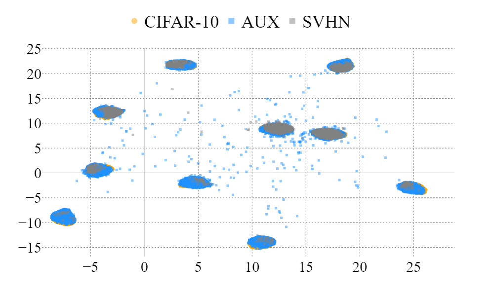
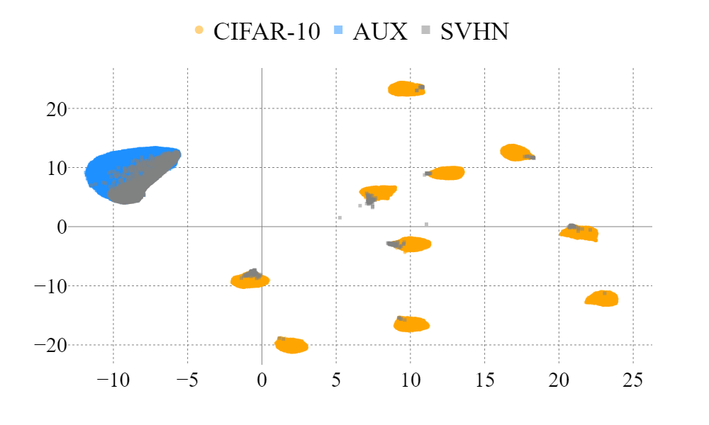
(a) without Hopfield Boosting
Refer to caption
(b) with Hopfield Boosting
Refer to caption
Figure 9: UMAP embeddings of ID (CIFAR-10) and OOD (AUX and SVHN) data based on our model trained without (a) and with Hopfield Boosting (b). Clearly, without Hopfield Boosting, the embedded OOD data points tend to overlap with the ID data points, making it impossible to distinguish between ID and OOD. On the other hand, Hopfield Boosting shows a clear separation of ID and OOD data in the embedding.

F.4 OOD Examples from the Places 365 Data Set with High Semantic Similarity to CIFAR-10

We observe that Hopfield Boosting and all competing methods struggle with correctly classifying the samples from the Places 365 data set as OOD the most. Table 1 shows that for Hopfield Boosting, the FPR95 for the Places 365 data set with CIFAR-10 as the ID data set is at 4.28. The second worst FPR95 for Hopfield Boosting was measured on the LSUN-Crop data set at 0.82.

We inspect the 100 images from Places 365 that perform worst (i.e., that achieve the highest score s(𝝃)𝑠𝝃s(\bm{\xi})) on a model trained with Hopfield Boosting on the CIFAR-10 data set as the in-distribution data set. Figure 10 shows that within those 100 images, the Places 365 data set contains a non-negligible amount of data instances that show objects from semantic classes contained in CIFAR-10 (e.g., horses, automobiles, dogs, trucks, and airplanes). We argue that data instances that clearly show objects of semantic classes contained in CIFAR-10 should be considered as in-distribution, which Hopfield Boosting correctly recognizes. Therefore, a certain amount of error can be anticipated on the Places 365 data set for all OOD detection methods. We leave a closer evaluation of the amount of the anticipated error up to future work.

For comparison, Figure 11 shows the 100 images from Places 365 with the lowest score s(𝝃)𝑠𝝃s(\bm{\xi}), as evaluated by a model trained with Hopfield Boosting on CIFAR-10. There are no objects visible that have clear semantic overlap with the CIFAR-10 classes.
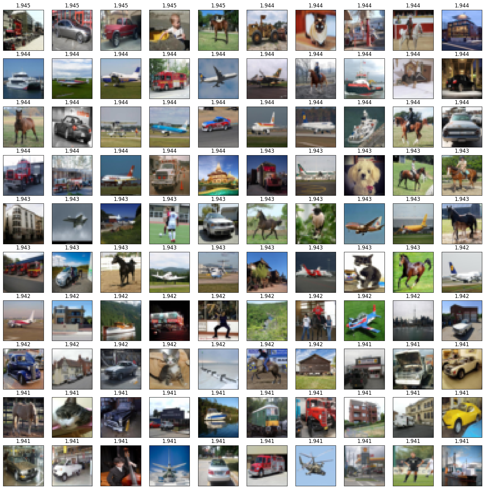
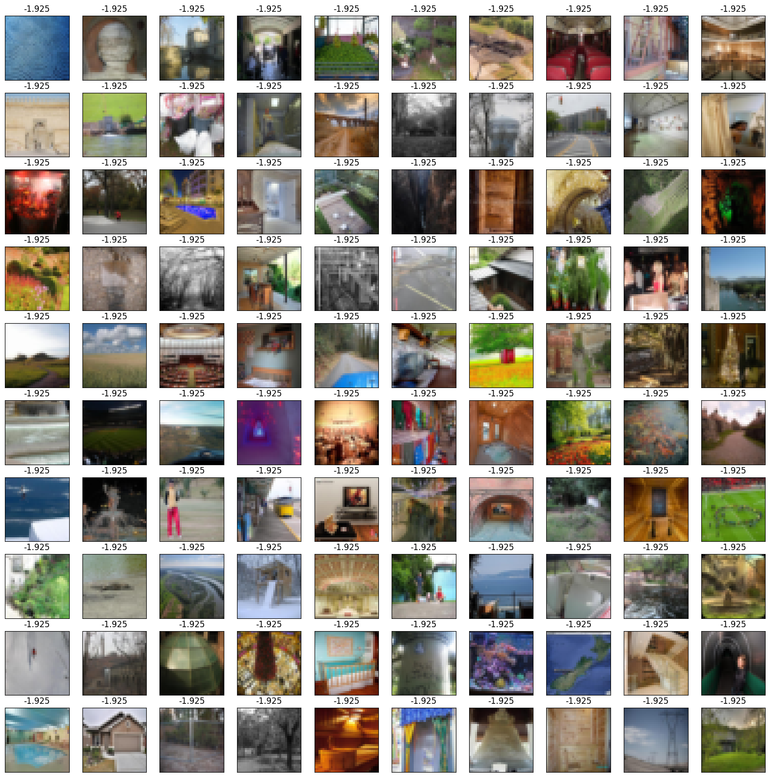
Refer to caption
Figure 10: The set of top-100 images from the Places 365 data set which Hopfield Boosting recognized as in-distribution. The image captions show s(𝝃)𝑠𝝃s(\bm{\xi}) of the respective image below the caption.
Refer to caption
Figure 11: The set of top-100 images from the Places 365 data set which Hopfield Boosting recognized as out-of-distribution. The image captions show s(𝝃)𝑠𝝃s(\bm{\xi}) of the respective image below the caption.

F.5 Results on Noticeably Different Data Sets

The choice of additional data sets should not be driven by a desire to showcase good performance; rather, we suggest opting for data that highlights weaknesses, as it holds the potential to drive investigations and uncover novel insights. Simple toy data is preferable due to its typically clearer and more intuitive characteristics compared to complex natural image data. In alignment with these considerations, the following data sets captivated our interest: iCartoonFace (Zheng et al., 2020), Four Shapes (smeschke, 2018), and Retail Product Checkout (RPC) (Wei et al., 2022b). In Figure 12, we show random samples from these data sets to demonstrate the noticeable differences compared to CIFAR-10.

Refer to caption
Figure 12: Random samples from three data sets, each noticeably different from CIFAR-10. First row: iCartoonFace; Second row: Four shapes; Third row: RPC.
Table 7: Comparison between EBO-OE (Liu et al., 2020) and our version. \downarrow indicates “lower is better” and \uparrow indicates “higher is better”.

Hopfield Boosting EBO-OE
OOD Dataset FPR95 \downarrow AUROC \uparrow FPR95 \downarrow AUROC \uparrow
iCartoonFace 0.600.60\mathbf{0.60} 99.5799.57\mathbf{99.57} 4.014.014.01 98.9498.9498.94
Four Shapes 40.8140.81\mathbf{40.81} 90.5390.53\mathbf{90.53} 62.5562.5562.55 75.3475.3475.34
RPC 4.074.07\mathbf{4.07} 98.6598.65\mathbf{98.65} 18.5118.5118.51 96.1096.1096.10

In Table 7, we present some preliminary results using models trained with the respective method on CIFAR-10 as ID data set (as in Table 1). Results for comparison are presented for EBO only, as time constraints prevented experimenting with additional baseline methods. Although one would expect near-perfect results due to the evident disparities with CIFAR-10, Four Shapes (smeschke, 2018) and RPC (Wei et al., 2022b) seem to defy that expectation. Their results indicate a weakness in the capability to identify outliers robustly since many samples are classified as inliers. Only iCartoonFace (Zheng et al., 2020) is correctly detected as OOD, at least to a large degree. Interestingly, the weakness uncovered by this data is present in both methods, although more pronounced in EBO-OE. Therefore, we suspect that this specific behavior may be a general weakness when training OOD detectors using OE, an aspect we plan to investigate further in our future work.

F.6 Runtime Considerations for Inference

When using Hopfield Boosting in inference, an additional inference step is needed to check whether a given sample is ID or OOD. Namely, to obtain the score (Equation (13)) of a query sample 𝝃𝒟superscript𝝃𝒟\bm{\xi}^{\mathcal{D}}, Hopfield Boosting computes the dot product similarity of the embedding obtained from 𝝃=ϕ(𝝃𝒟)𝝃italic-ϕsuperscript𝝃𝒟\bm{\xi}\ =\ \phi(\bm{\xi}^{\mathcal{D}}) to all samples in the Hopfield memories 𝑿𝑿\bm{X} and 𝑶𝑶\bm{O}. In our experiments, 𝑿𝑿\bm{X} contains the full in-distribution data set (50,000 samples) and 𝑶𝑶\bm{O} contains a subset of the AUX data set of equal size. We investigate the computational overhead of computing the dot-product similarity to 100,000 samples in relation to the computational load of the encoder. For this, we feed 100 batches of size 1024 to an encoder (1) without using the score and (2) with using the score, measure the runtimes per batch, and compute the mean and standard deviation. We conduct this experiment with four different encoders on an NVIDIA Titan V GPU. The results are shown in Figure 13 and Table 8. One can see that, especially for larger models, the computational overhead of determining the score is very moderate in comparison.
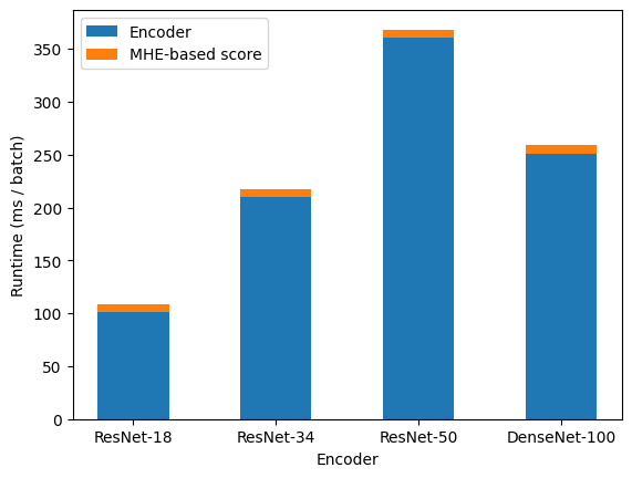
Refer to caption
Figure 13: Mean inference runtimes for Hopfield Boosting on four different encoders on an NVIDIA Titan V GPU. We plot the contributions to the total runtime of the encoder and the MHE-based score (Equation (13)) separately. The evaluation shows that the score computation adds a negligible amount of computational overhead to the total runtime.
Table 8: Inference runtimes for Hopfield Boosting with four different encoders on an NVIDIA Titan V GPU. We compare the runtime of the encoder only and the runtime of the encoder with the MHE-based score computation (Equation (13)) combined.

Encoder Time encoder (ms / batch) Time encoder + score (ms / batch) Rel. overhead (%)
ResNet-18 100.93±0.24superscript100.93plus-or-minus0.24100.93^{\pm 0.24} 108.50±0.19superscript108.50plus-or-minus0.19108.50^{\pm 0.19} 7.507.507.50
ResNet-34 209.80±0.40superscript209.80plus-or-minus0.40209.80^{\pm 0.40} 217.33±0.51superscript217.33plus-or-minus0.51217.33^{\pm 0.51} 3.593.593.59
ResNet-50 360.93±1.51superscript360.93plus-or-minus1.51360.93^{\pm 1.51} 368.17±0.62superscript368.17plus-or-minus0.62368.17^{\pm 0.62} 2.012.012.01
Densenet-100 251.24±1.36superscript251.24plus-or-minus1.36251.24^{\pm 1.36} 258.82±0.84superscript258.82plus-or-minus0.84258.82^{\pm 0.84} 3.023.023.02

F.7 Non-OE Baselines

To confirm the prevailing notion that OE methods can improve the OOD detection capability in general, we compare Hopfield Boosting to 3 training methods (Sehwag et al., 2021; Tao et al., 2023; Lu et al., 2024) and 5 post-hoc methods (Hendrycks & Gimpel, 2017; Hendrycks et al., 2019b; Liu et al., 2020, 2023; Djurisic et al., 2023). For all methods, we train a ResNet-18 on CIFAR-10. For Hopfield Boosting, we use the same training setup as described in section 5.1. For the post-hoc methods, we do not use the auxiliary outlier data. For the training methods, we use the training procedures described in the respective publications for 100 epochs. Notably, all training methods employ stronger augmentations than the OE or the post-hoc methods. The OE and post-hoc methods use the following augmentations (denoted as “Weak”):

  1. 1.

    RandomCrop (32x32), padding 4

  2. 2.

    RandomHorizontalFlip

The training methods use the following augmentations (denoted as “Strong”):

  1. 1.

    RandomResizedCrop (32x32), scale 0.2-1

  2. 2.

    RandomHorizontalFlip

  3. 3.

    ColorJitter applied with probability 0.8

  4. 4.

    RandomGrayscale applied with probability 0.2

Table F.7 shows the results of the comparison of Hopfield Boosting to the post-hoc and training methods. Hopfield Boosting is better at OOD detection than all non-OE baselines on CIFAR-10 in terms of both mean AUROC and mean FPR95 by a large margin. Further, Hopfield Boosting achieves the best OOD detection on all OOD data sets in terms of FPR95 and AUROC, except for SVHN and LSUN-Crop, where PALM (Lu et al., 2024) shows better AUROC results. An interesting avenue for future work is to combine one of the non-OE based training methods with the OE method Hopfield Boosting.


Table 9: OOD detection performance on CIFAR-10. We compare results from Hopfield Boosting, PALM (Lu et al., 2024), NPOS (Tao et al., 2023), SSD+ (Sehwag et al., 2021), ASH (Djurisic et al., 2023), GEN (Liu et al., 2023), EBO (Liu et al., 2020), MaxLogit (Hendrycks et al., 2019a), and MSP (Hendrycks & Gimpel, 2017) on ResNet-18. \downarrow indicates “lower is better” and \uparrow “higher is better”. All values in %percent\%. Standard deviations are estimated across five training runs.
HB (ours) PALM NPOS SSD+ ASH GEN EBO MaxLogit MSP
\rowcolorgray!25 FPR95 \downarrow 0.23±0.08superscript0.23plus-or-minus0.08\mathbf{0.23^{\pm 0.08}} 1.24±0.49superscript1.24plus-or-minus0.491.24^{\pm 0.49} 9.04±1.13superscript9.04plus-or-minus1.139.04^{\pm 1.13} 3.05±0.22superscript3.05plus-or-minus0.223.05^{\pm 0.22} 25.17±9.55superscript25.17plus-or-minus9.5525.17^{\pm 9.55} 33.26±5.99superscript33.26plus-or-minus5.9933.26^{\pm 5.99} 32.10±6.41superscript32.10plus-or-minus6.4132.10^{\pm 6.41} 33.27±6.18superscript33.27plus-or-minus6.1833.27^{\pm 6.18} 49.41±3.77superscript49.41plus-or-minus3.7749.41^{\pm 3.77}
\rowcolorgray!25 SVHN AUROC \uparrow 99.57±0.06superscript99.57plus-or-minus0.0699.57^{\pm 0.06} 99.70±0.12superscript99.70plus-or-minus0.12\mathbf{99.70^{\pm 0.12}} 98.37±0.23superscript98.37plus-or-minus0.2398.37^{\pm 0.23} 99.41±0.06superscript99.41plus-or-minus0.0699.41^{\pm 0.06} 94.86±2.09superscript94.86plus-or-minus2.0994.86^{\pm 2.09} 93.53±1.42superscript93.53plus-or-minus1.4293.53^{\pm 1.42} 93.43±1.60superscript93.43plus-or-minus1.6093.43^{\pm 1.60} 93.29±1.57superscript93.29plus-or-minus1.5793.29^{\pm 1.57} 92.48±0.93superscript92.48plus-or-minus0.9392.48^{\pm 0.93}
\rowcolorwhite FPR95 \downarrow 0.82±0.17superscript0.82plus-or-minus0.17\mathbf{0.82^{\pm 0.17}} 1.21±0.27superscript1.21plus-or-minus0.271.21^{\pm 0.27} 5.52±0.50superscript5.52plus-or-minus0.505.52^{\pm 0.50} 2.83±1.10superscript2.83plus-or-minus1.102.83^{\pm 1.10} 13.13±1.81superscript13.13plus-or-minus1.8113.13^{\pm 1.81} 19.40±2.22superscript19.40plus-or-minus2.2219.40^{\pm 2.22} 17.25±2.30superscript17.25plus-or-minus2.3017.25^{\pm 2.30} 18.50±2.24superscript18.50plus-or-minus2.2418.50^{\pm 2.24} 38.32±2.61superscript38.32plus-or-minus2.6138.32^{\pm 2.61}
\rowcolorwhite LSUN-Crop AUROC \uparrow 99.40±0.04superscript99.40plus-or-minus0.0499.40^{\pm 0.04} 99.65±0.05superscript99.65plus-or-minus0.05\mathbf{99.65^{\pm 0.05}} 98.97±0.04superscript98.97plus-or-minus0.0498.97^{\pm 0.04} 99.37±0.16superscript99.37plus-or-minus0.1699.37^{\pm 0.16} 97.33±0.36superscript97.33plus-or-minus0.3697.33^{\pm 0.36} 96.48±0.46superscript96.48plus-or-minus0.4696.48^{\pm 0.46} 96.73±0.46superscript96.73plus-or-minus0.4696.73^{\pm 0.46} 96.52±0.47superscript96.52plus-or-minus0.4796.52^{\pm 0.47} 94.37±0.53superscript94.37plus-or-minus0.5394.37^{\pm 0.53}
\rowcolorgray!25 FPR95 \downarrow 0.00±0.00superscript0.00plus-or-minus0.00\mathbf{0.00^{\pm 0.00}} 27.01±5.82superscript27.01plus-or-minus5.8227.01^{\pm 5.82} 26.85±3.14superscript26.85plus-or-minus3.1426.85^{\pm 3.14} 34.30±2.17superscript34.30plus-or-minus2.1734.30^{\pm 2.17} 38.18±5.78superscript38.18plus-or-minus5.7838.18^{\pm 5.78} 31.50±3.92superscript31.50plus-or-minus3.9231.50^{\pm 3.92} 30.69±4.03superscript30.69plus-or-minus4.0330.69^{\pm 4.03} 31.64±4.01superscript31.64plus-or-minus4.0131.64^{\pm 4.01} 45.82±3.48superscript45.82plus-or-minus3.4845.82^{\pm 3.48}
\rowcolorgray!25 LSUN-Resize AUROC \uparrow 99.98±0.02superscript99.98plus-or-minus0.02\mathbf{99.98^{\pm 0.02}} 95.41±0.74superscript95.41plus-or-minus0.7495.41^{\pm 0.74} 95.68±0.36superscript95.68plus-or-minus0.3695.68^{\pm 0.36} 94.78±0.25superscript94.78plus-or-minus0.2594.78^{\pm 0.25} 90.39±2.00superscript90.39plus-or-minus2.0090.39^{\pm 2.00} 94.04±0.84superscript94.04plus-or-minus0.8494.04^{\pm 0.84} 94.02±0.86superscript94.02plus-or-minus0.8694.02^{\pm 0.86} 93.90±0.86superscript93.90plus-or-minus0.8693.90^{\pm 0.86} 92.84±0.80superscript92.84plus-or-minus0.8092.84^{\pm 0.80}
\rowcolorwhite FPR95 \downarrow 0.16±0.02superscript0.16plus-or-minus0.02\mathbf{0.16^{\pm 0.02}} 17.32±2.50superscript17.32plus-or-minus2.5017.32^{\pm 2.50} 27.72±2.55superscript27.72plus-or-minus2.5527.72^{\pm 2.55} 21.20±2.20superscript21.20plus-or-minus2.2021.20^{\pm 2.20} 46.08±6.22superscript46.08plus-or-minus6.2246.08^{\pm 6.22} 44.62±4.14superscript44.62plus-or-minus4.1444.62^{\pm 4.14} 44.67±4.46superscript44.67plus-or-minus4.4644.67^{\pm 4.46} 44.97±4.44superscript44.97plus-or-minus4.4444.97^{\pm 4.44} 55.04±2.86superscript55.04plus-or-minus2.8655.04^{\pm 2.86}
\rowcolorwhite Textures AUROC \uparrow 99.84±0.01superscript99.84plus-or-minus0.01\mathbf{99.84^{\pm 0.01}} 96.82±0.71superscript96.82plus-or-minus0.7196.82^{\pm 0.71} 95.36±0.35superscript95.36plus-or-minus0.3595.36^{\pm 0.35} 96.46±0.35superscript96.46plus-or-minus0.3596.46^{\pm 0.35} 88.32±2.08superscript88.32plus-or-minus2.0888.32^{\pm 2.08} 90.12±1.32superscript90.12plus-or-minus1.3290.12^{\pm 1.32} 89.61±1.50superscript89.61plus-or-minus1.5089.61^{\pm 1.50} 89.56±1.48superscript89.56plus-or-minus1.4889.56^{\pm 1.48} 90.10±0.92superscript90.10plus-or-minus0.9290.10^{\pm 0.92}
\rowcolorgray!25 FPR95 \downarrow 0.00±0.00superscript0.00plus-or-minus0.00\mathbf{0.00^{\pm 0.00}} 25.71±4.83superscript25.71plus-or-minus4.8325.71^{\pm 4.83} 26.90±3.52superscript26.90plus-or-minus3.5226.90^{\pm 3.52} 35.71±2.27superscript35.71plus-or-minus2.2735.71^{\pm 2.27} 42.41±6.28superscript42.41plus-or-minus6.2842.41^{\pm 6.28} 35.85±4.05superscript35.85plus-or-minus4.0535.85^{\pm 4.05} 34.99±4.33superscript34.99plus-or-minus4.3334.99^{\pm 4.33} 36.02±4.18superscript36.02plus-or-minus4.1836.02^{\pm 4.18} 49.10±3.06superscript49.10plus-or-minus3.0649.10^{\pm 3.06}
\rowcolorgray!25 iSUN AUROC \uparrow 99.97±0.02superscript99.97plus-or-minus0.02\mathbf{99.97^{\pm 0.02}} 95.60±0.65superscript95.60plus-or-minus0.6595.60^{\pm 0.65} 95.74±0.38superscript95.74plus-or-minus0.3895.74^{\pm 0.38} 94.49±0.25superscript94.49plus-or-minus0.2594.49^{\pm 0.25} 89.06±2.26superscript89.06plus-or-minus2.2689.06^{\pm 2.26} 93.05±0.84superscript93.05plus-or-minus0.8493.05^{\pm 0.84} 92.99±0.90superscript92.99plus-or-minus0.9092.99^{\pm 0.90} 92.88±0.90superscript92.88plus-or-minus0.9092.88^{\pm 0.90} 91.99±0.74superscript91.99plus-or-minus0.7491.99^{\pm 0.74}
\rowcolorwhite FPR95 \downarrow 4.28±0.23superscript4.28plus-or-minus0.23\mathbf{4.28^{\pm 0.23}} 22.97±2.17superscript22.97plus-or-minus2.1722.97^{\pm 2.17} 32.62±0.13superscript32.62plus-or-minus0.1332.62^{\pm 0.13} 24.99±1.21superscript24.99plus-or-minus1.2124.99^{\pm 1.21} 48.03±2.04superscript48.03plus-or-minus2.0448.03^{\pm 2.04} 45.82±1.07superscript45.82plus-or-minus1.0745.82^{\pm 1.07} 44.87±1.11superscript44.87plus-or-minus1.1144.87^{\pm 1.11} 45.63±1.26superscript45.63plus-or-minus1.2645.63^{\pm 1.26} 57.58±0.97superscript57.58plus-or-minus0.9757.58^{\pm 0.97}
\rowcolorwhite Places 365 AUROC \uparrow 98.51±0.10superscript98.51plus-or-minus0.10\mathbf{98.51^{\pm 0.10}} 94.95±0.53superscript94.95plus-or-minus0.5394.95^{\pm 0.53} 93.76±0.12superscript93.76plus-or-minus0.1293.76^{\pm 0.12} 94.93±0.22superscript94.93plus-or-minus0.2294.93^{\pm 0.22} 85.65±0.77superscript85.65plus-or-minus0.7785.65^{\pm 0.77} 88.68±0.28superscript88.68plus-or-minus0.2888.68^{\pm 0.28} 88.53±0.30superscript88.53plus-or-minus0.3088.53^{\pm 0.30} 88.42±0.29superscript88.42plus-or-minus0.2988.42^{\pm 0.29} 88.06±0.25superscript88.06plus-or-minus0.2588.06^{\pm 0.25}
\rowcolorwhite FPR95 \downarrow 0.920.92\mathbf{0.92} 15.9115.9115.91 21.4421.4421.44 20.3520.3520.35 35.5035.5035.50 35.0735.0735.07 34.0934.0934.09 35.0035.0035.00 49.2149.2149.21
\rowcolorwhite Mean AUROC \uparrow 99.5599.55\mathbf{99.55} 97.0297.0297.02 96.3196.3196.31 96.5796.5796.57 90.9490.9490.94 92.6592.6592.65 92.5592.5592.55 92.4392.4392.43 91.6491.6491.64
\rowcolorgray!25     Method type OE Training Training Training Post-hoc Post-hoc Post-hoc Post-hoc Post-hoc
\rowcolorgray!25     Augmentations Weak Strong Strong Strong Weak Weak Weak Weak Weak
\rowcolorgray!25     Auxiliary outlier data

Appendix G Informativeness of Sampling with High Boundary Scores

This section adopts and expands the arguments of Ming et al. (2022) on sampling with high boundary scores.

We assume the extracted features of a trained deep neural network to approximately equal a Gaussian mixture model with equal class priors:

p(𝝃)𝑝𝝃\displaystyle p(\bm{\xi})\ =12𝒩(𝝃;𝝁,σ2𝑰)+12𝒩(𝝃;𝝁,σ2𝑰)absent12𝒩𝝃𝝁superscript𝜎2𝑰12𝒩𝝃𝝁superscript𝜎2𝑰\displaystyle=\ \frac{1}{2}\mathcal{N}(\bm{\xi};\bm{\mu},\sigma^{2}\bm{I})+\frac{1}{2}\mathcal{N}(\bm{\xi};-\bm{\mu},\sigma^{2}\bm{I}) (125)
pID(𝝃)=p(𝝃|ID)subscript𝑝ID𝝃𝑝conditional𝝃ID\displaystyle p_{\text{ID}}(\bm{\xi})=p(\bm{\xi}|\text{ID})\ =𝒩(𝝃;𝝁,σ2𝑰)absent𝒩𝝃𝝁superscript𝜎2𝑰\displaystyle=\ \mathcal{N}(\bm{\xi};\bm{\mu},\sigma^{2}\bm{I}) (126)
pAUX(𝝃)=p(𝝃|AUX)subscript𝑝AUX𝝃𝑝conditional𝝃AUX\displaystyle p_{\text{AUX}}(\bm{\xi})=p(\bm{\xi}|\text{AUX})\ =𝒩(𝝃;𝝁,σ2𝑰)absent𝒩𝝃𝝁superscript𝜎2𝑰\displaystyle=\ \mathcal{N}(\bm{\xi};-\bm{\mu},\sigma^{2}\bm{I}) (127)

Using the MHE and sufficient data from those distributions, we can estimate the densities p(𝝃)𝑝𝝃p(\bm{\xi}), p(𝝃|ID)𝑝conditional𝝃IDp(\bm{\xi}|\text{ID}) and p(𝝃|AUX)𝑝conditional𝝃AUXp(\bm{\xi}|\text{AUX}).

Lemma G.1.

(see Lemma E.1 in Ming et al. (2022)) Assume the M sampled data points 𝐨ipAUXsimilar-tosubscript𝐨𝑖subscript𝑝AUX\bm{o}_{i}\sim p_{\text{AUX}} satisfy the following constraint on high boundary scores Eb(𝛏)subscriptE𝑏𝛏\mathrm{E}_{b}(\bm{\xi})

i=1MEb(𝒐i)Mϵsuperscriptsubscript𝑖1𝑀subscriptE𝑏subscript𝒐𝑖𝑀italic-ϵ\displaystyle\frac{-\sum_{i=1}^{M}\mathrm{E}_{b}(\bm{o}_{i})}{M}\leq\epsilon (128)

Then they have

i=1M|2𝝁T𝒐i|Mϵσ2superscriptsubscript𝑖1𝑀2superscript𝝁𝑇subscript𝒐𝑖𝑀italic-ϵsuperscript𝜎2\displaystyle\sum_{i=1}^{M}|2\bm{\mu}^{T}\bm{o}_{i}|\leq M\epsilon\sigma^{2} (129)
Proof.

They first obtain the expression for Eb(𝝃)subscriptE𝑏𝝃\mathrm{E}_{b}(\bm{\xi}) under the Gaussian mixture model described above and can express p(AUX|𝝃)𝑝conditionalAUX𝝃p(\text{AUX}|\bm{\xi}) as

p(AUX|𝝃)𝑝conditionalAUX𝝃\displaystyle p(\text{AUX}|\bm{\xi})\ =p(𝝃|AUX)p(AUX)p(𝝃)absent𝑝conditional𝝃AUX𝑝AUX𝑝𝝃\displaystyle=\ \frac{p(\bm{\xi}|\text{AUX})p(\text{AUX})}{p(\bm{\xi})} (130)
=12p(𝝃|AUX)12p(𝝃|ID)+12p(𝝃|AUX)absent12𝑝conditional𝝃AUX12𝑝conditional𝝃ID12𝑝conditional𝝃AUX\displaystyle=\ \frac{\frac{1}{2}p(\bm{\xi}|\text{AUX})}{\frac{1}{2}p(\bm{\xi}|\text{ID})\ +\ \frac{1}{2}p(\bm{\xi}|\text{AUX})} (131)
=(2πσ2)d/2exp(12σ2𝝃𝝁22)(2πσ2)d/2exp(12σ2𝝃+𝝁22)+(2πβ1)d/2exp(12σ2𝝃𝝁22)absentsuperscript2𝜋superscript𝜎2𝑑212superscript𝜎2superscriptsubscriptnorm𝝃𝝁22superscript2𝜋superscript𝜎2𝑑212superscript𝜎2superscriptsubscriptnorm𝝃𝝁22superscript2𝜋superscript𝛽1𝑑212superscript𝜎2superscriptsubscriptnorm𝝃𝝁22\displaystyle=\ \frac{(2\pi\sigma^{2})^{-d/2}\exp(-\frac{1}{2\sigma^{2}}||\bm{\xi}-\bm{\mu}||_{2}^{2})}{(2\pi\sigma^{2})^{-d/2}\exp(-\frac{1}{2\sigma^{2}}||\bm{\xi}+\bm{\mu}||_{2}^{2})\ +\ (2\pi\beta^{-1})^{-d/2}\exp(-\frac{1}{2\sigma^{2}}||\bm{\xi}-\bm{\mu}||_{2}^{2})} (132)
=11+exp(12σ2(𝝃𝝁22𝝃+𝝁22))absent1112superscript𝜎2superscriptsubscriptnorm𝝃𝝁22superscriptsubscriptnorm𝝃𝝁22\displaystyle=\ \frac{1}{1\ +\ \exp(-\frac{1}{2\sigma^{2}}(||\bm{\xi}-\bm{\mu}||_{2}^{2}-||\bm{\xi}+\bm{\mu}||_{2}^{2}))} (133)

When defining fAUX(𝝃)=12σ2(𝝃𝝁22𝝃+𝝁22)subscript𝑓AUX𝝃12superscript𝜎2superscriptsubscriptnorm𝝃𝝁22superscriptsubscriptnorm𝝃𝝁22f_{\text{AUX}}(\bm{\xi})\ =\ \frac{1}{2\sigma^{2}}(||\bm{\xi}-\bm{\mu}||_{2}^{2}-||\bm{\xi}+\bm{\mu}||_{2}^{2}) such that p(AUX|𝝃)=σ(fAUX(𝝃))=11+exp(fAUX(𝝃))𝑝conditionalAUX𝝃𝜎subscript𝑓AUX𝝃11subscript𝑓AUX𝝃p(\text{AUX}|\bm{\xi})\ =\sigma(f_{\text{AUX}}(\bm{\xi}))\ =\ \frac{1}{1\ +\ \exp(-f_{\text{AUX}}(\bm{\xi}))}, they define EbsubscriptE𝑏\mathrm{E}_{b} as follows:

Eb(𝝃)subscriptE𝑏𝝃\displaystyle\mathrm{E}_{b}(\bm{\xi})\ =|fAUX(𝝃)|absentsubscript𝑓AUX𝝃\displaystyle=\ -|f_{\text{AUX}}(\bm{\xi})| (134)
=12σ2|𝝃𝝁22𝝃+𝝁22|absent12superscript𝜎2superscriptsubscriptnorm𝝃𝝁22superscriptsubscriptnorm𝝃𝝁22\displaystyle=\ -\frac{1}{2\sigma^{2}}|\ ||\bm{\xi}-\bm{\mu}||_{2}^{2}-||\bm{\xi}+\bm{\mu}||_{2}^{2}\ | (135)
=12σ2|𝝃T𝝃2𝝁T𝝃+𝝁T𝝁(𝝃T𝝃+2𝝁T𝝃+𝝁T𝝁)|absent12superscript𝜎2superscript𝝃𝑇𝝃2superscript𝝁𝑇𝝃superscript𝝁𝑇𝝁superscript𝝃𝑇𝝃2superscript𝝁𝑇𝝃superscript𝝁𝑇𝝁\displaystyle=\ -\frac{1}{2\sigma^{2}}|\ \bm{\xi}^{T}\bm{\xi}-2\bm{\mu}^{T}\bm{\xi}+\bm{\mu}^{T}\bm{\mu}-(\bm{\xi}^{T}\bm{\xi}+2\bm{\mu}^{T}\bm{\xi}+\bm{\mu}^{T}\bm{\mu})| (136)
=|2𝝁T𝝃|σ2absent2superscript𝝁𝑇𝝃superscript𝜎2\displaystyle=-\frac{|2\bm{\mu}^{T}\bm{\xi}|}{\sigma^{2}} (137)

Therefore, the constraint in Equation (129) is translated to

i=1M|2𝝁T𝒐i|Mϵσ2superscriptsubscript𝑖1𝑀2superscript𝝁𝑇subscript𝒐𝑖𝑀italic-ϵsuperscript𝜎2\displaystyle\sum_{i=1}^{M}|2\bm{\mu}^{T}\bm{o}_{i}|\ \leq\ M\epsilon\sigma^{2} (138)

As maxiM|𝝁T𝒐i|i=1M|𝝁T𝒐i|subscript𝑖𝑀superscript𝝁𝑇subscript𝒐𝑖superscriptsubscript𝑖1𝑀superscript𝝁𝑇subscript𝒐𝑖\max_{i\in M}|\bm{\mu}^{T}\bm{o}_{i}|\leq\sum_{i=1}^{M}|\bm{\mu}^{T}\bm{o}_{i}| given a fixed M𝑀M, the selected samples can be seen as generated from pAUXsubscript𝑝AUXp_{\text{AUX}} with the constraint that all samples lie within the two hyperplanes in Equation (138)italic-(138italic-)\eqref{eqn:boundary-contraint-translated}.

Parameter estimation.

Now they show the benefit of such constraint in controlling the sample complexity. Assume the signal/noise ratio is large: 𝝁σ=r1norm𝝁𝜎𝑟much-greater-than1\frac{||\bm{\mu}||}{\sigma}=r\gg 1, and ϵ1italic-ϵ1\epsilon\leq 1 is some constant.

Assume the classifier is given by

𝜽=1N+M(i=1M𝒙ii=1N𝒐i)𝜽1𝑁𝑀superscriptsubscript𝑖1𝑀subscript𝒙𝑖superscriptsubscript𝑖1𝑁subscript𝒐𝑖\displaystyle\bm{\theta}\ =\ \frac{1}{N+M}(\sum_{i=1}^{M}\bm{x}_{i}-\sum_{i=1}^{N}\bm{o}_{i}) (139)

where 𝒐ipAUXsimilar-tosubscript𝒐𝑖subscript𝑝AUX\bm{o}_{i}\sim p_{\text{AUX}} and 𝒙ipIDsimilar-tosubscript𝒙𝑖subscript𝑝ID\bm{x}_{i}\sim p_{\text{ID}}. One can decompose 𝜽𝜽\bm{\theta}. Assuming M=N𝑀𝑁M=N:

𝜽=𝝁+12𝜼+12𝝎𝜽𝝁12𝜼12𝝎\displaystyle\bm{\theta}=\bm{\mu}+\frac{1}{2}\bm{\eta}+\frac{1}{2}\bm{\omega} (140)
𝜼=1N(i=1N𝒙i)𝝁𝜼1𝑁superscriptsubscript𝑖1𝑁subscript𝒙𝑖𝝁\displaystyle\bm{\eta}\ =\ \frac{1}{N}(\sum_{i=1}^{N}\bm{x}_{i})-\bm{\mu} (141)
𝝎=1N(i=1M𝒐i)𝝁𝝎1𝑁superscriptsubscript𝑖1𝑀subscript𝒐𝑖𝝁\displaystyle\bm{\omega}\ =\ \frac{1}{N}(\sum_{i=1}^{M}-\ \bm{o}_{i})-\bm{\mu} (142)

We would now like to determine the distributions of the random variables 𝜼22superscriptsubscriptnorm𝜼22||\bm{\eta}||_{2}^{2} and 𝝁T𝜼superscript𝝁𝑇𝜼\bm{\mu}^{T}\bm{\eta}

𝜼22superscriptsubscriptnorm𝜼22\displaystyle||\bm{\eta}||_{2}^{2} =i=1dηi2absentsuperscriptsubscript𝑖1𝑑superscriptsubscript𝜂𝑖2\displaystyle=\sum_{i=1}^{d}\eta_{i}^{2} (143)
ηisubscript𝜂𝑖\displaystyle\eta_{i}\ 𝒩(0,σ2N)similar-toabsent𝒩0superscript𝜎2𝑁\displaystyle\sim\mathcal{N}(0,\frac{\sigma^{2}}{N}) (144)
Nσηi𝑁𝜎subscript𝜂𝑖\displaystyle\frac{\sqrt{N}}{\sigma}\eta_{i}\ 𝒩(0,1)similar-toabsent𝒩01\displaystyle\sim\ \mathcal{N}(0,1) (145)
(Nσηi)2superscript𝑁𝜎subscript𝜂𝑖2\displaystyle(\frac{\sqrt{N}}{\sigma}\eta_{i})^{2}\ χ12similar-toabsentsubscriptsuperscript𝜒21\displaystyle\sim\ \chi^{2}_{1} (146)

Therefore, for 𝜼22superscriptsubscriptnorm𝜼22||\bm{\eta}||_{2}^{2} we have

Nσ2𝜼22𝑁superscript𝜎2superscriptsubscriptnorm𝜼22\displaystyle\frac{N}{\sigma^{2}}||\bm{\eta}||_{2}^{2} =i=1d(Nσηi)2χd2absentsuperscriptsubscript𝑖1𝑑superscript𝑁𝜎subscript𝜂𝑖2similar-tosubscriptsuperscript𝜒2𝑑\displaystyle=\sum_{i=1}^{d}(\frac{\sqrt{N}}{\sigma}\eta_{i})^{2}\ \sim\ \chi^{2}_{d} (147)

Now we would like to determine the distribution of 𝝁T𝜼superscript𝝁𝑇𝜼\bm{\mu}^{T}\bm{\eta}:

𝝁T𝜼superscript𝝁𝑇𝜼\displaystyle\bm{\mu}^{T}\bm{\eta}\ =i=1dμiηiabsentsuperscriptsubscript𝑖1𝑑subscript𝜇𝑖subscript𝜂𝑖\displaystyle=\ \sum_{i=1}^{d}\mu_{i}\ \eta_{i} (148)
μiηisubscript𝜇𝑖subscript𝜂𝑖\displaystyle\mu_{i}\ \eta_{i}\ 𝒩(0,σ2μi2N)similar-toabsent𝒩0superscript𝜎2superscriptsubscript𝜇𝑖2𝑁\displaystyle\sim\ \mathcal{N}(0,\frac{\sigma^{2}\mu_{i}^{2}}{N}) (149)
i=1dμiηisuperscriptsubscript𝑖1𝑑subscript𝜇𝑖subscript𝜂𝑖\displaystyle\sum_{i=1}^{d}\mu_{i}\ \eta_{i}\ 𝒩(0,i=1dσ2μi2N)similar-toabsent𝒩0superscriptsubscript𝑖1𝑑superscript𝜎2superscriptsubscript𝜇𝑖2𝑁\displaystyle\sim\ \mathcal{N}(0,\sum_{i=1}^{d}\frac{\sigma^{2}\mu_{i}^{2}}{N}) (150)
i=1dμiηisuperscriptsubscript𝑖1𝑑subscript𝜇𝑖subscript𝜂𝑖\displaystyle\sum_{i=1}^{d}\mu_{i}\ \eta_{i}\ 𝒩(0,σ2Ni=1dμi2)similar-toabsent𝒩0superscript𝜎2𝑁superscriptsubscript𝑖1𝑑superscriptsubscript𝜇𝑖2\displaystyle\sim\ \mathcal{N}(0,\frac{\sigma^{2}}{N}\sum_{i=1}^{d}\mu_{i}^{2}) (151)
𝝁T𝜼𝝁superscript𝝁𝑇𝜼norm𝝁\displaystyle\frac{\bm{\mu}^{T}\bm{\eta}}{||\bm{\mu}||}\ 𝒩(0,σ2N)similar-toabsent𝒩0superscript𝜎2𝑁\displaystyle\sim\ \mathcal{N}(0,\frac{\sigma^{2}}{N}) (152)

Concentration bounds.

They now develop concentration bounds for 𝜼22superscriptsubscriptnorm𝜼22||\bm{\eta}||_{2}^{2} and 𝝁T𝜼superscript𝝁𝑇𝜼\bm{\mu}^{T}\bm{\eta}. First, we look at 𝜼22superscriptsubscriptnorm𝜼22||\bm{\eta}||_{2}^{2}. A concentration bound for χd2subscriptsuperscript𝜒2𝑑\chi^{2}_{d} is:

(Xd2dx+2x)exp(x)𝑋𝑑2𝑑𝑥2𝑥𝑥\displaystyle\mathbb{P}(X-d\geq 2\sqrt{dx}+2x)\leq\exp(-x) (153)

By assuming x=d8σ2𝑥𝑑8superscript𝜎2x=\frac{d}{8\sigma^{2}} we obtain

(Xd2dd8σ2+2d8σ2)𝑋𝑑2𝑑𝑑8superscript𝜎22𝑑8superscript𝜎2\displaystyle\mathbb{P}(X-d\geq 2\sqrt{d\frac{d}{8\sigma^{2}}}+2\frac{d}{8\sigma^{2}}) exp(d8σ2)absent𝑑8superscript𝜎2\displaystyle\leq\exp(-\frac{d}{8\sigma^{2}}) (154)
(Xd2σ+d4σ2+d)𝑋𝑑2𝜎𝑑4superscript𝜎2𝑑\displaystyle\mathbb{P}(X\geq\frac{d}{\sqrt{2}\sigma}+\frac{d}{4\sigma^{2}}+d) exp(d8σ2)absent𝑑8superscript𝜎2\displaystyle\leq\exp(-\frac{d}{8\sigma^{2}}) (155)
(Nσ2𝜼22d2σ+d4σ2+d)𝑁superscript𝜎2superscriptsubscriptnorm𝜼22𝑑2𝜎𝑑4superscript𝜎2𝑑\displaystyle\mathbb{P}(\frac{N}{\sigma^{2}}||\bm{\eta}||_{2}^{2}\geq\frac{d}{\sqrt{2}\sigma}+\frac{d}{4\sigma^{2}}+d) exp(d8σ2)absent𝑑8superscript𝜎2\displaystyle\leq\exp(-\frac{d}{8\sigma^{2}}) (156)
(𝜼22σ2N(d2σ+d4σ2+d))superscriptsubscriptnorm𝜼22superscript𝜎2𝑁𝑑2𝜎𝑑4superscript𝜎2𝑑\displaystyle\mathbb{P}(||\bm{\eta}||_{2}^{2}\geq\frac{\sigma^{2}}{N}(\frac{d}{\sqrt{2}\sigma}+\frac{d}{4\sigma^{2}}+d)) exp(d8σ2)absent𝑑8superscript𝜎2\displaystyle\leq\exp(-\frac{d}{8\sigma^{2}}) (157)

If d2𝑑2d\geq 2 we have that333Strictly, the bound is valid for d>2𝑑2d>\sqrt{2}

d2σ+d4σ2>1σ𝑑2𝜎𝑑4superscript𝜎21𝜎\displaystyle\frac{d}{\sqrt{2}\sigma}+\frac{d}{4\sigma^{2}}>\frac{1}{\sigma} (158)

and thus, the above bound can be simplified when assuming d2𝑑2d\geq 2 as follows:

(𝜼22σ2N(1σ+d))superscriptsubscriptnorm𝜼22superscript𝜎2𝑁1𝜎𝑑\displaystyle\mathbb{P}(||\bm{\eta}||_{2}^{2}\geq\frac{\sigma^{2}}{N}(\frac{1}{\sigma}+d)) exp(d8σ2)absent𝑑8superscript𝜎2\displaystyle\leq\exp(-\frac{d}{8\sigma^{2}}) (159)

For 𝝎22superscriptsubscriptnorm𝝎22||\bm{\omega}||_{2}^{2}, since all 𝒐isubscript𝒐𝑖\bm{o}_{i} is drawn i.i.d. from pAUXsubscript𝑝AUXp_{\text{AUX}}, under the constraint in Equation (138), the distribution of 𝝎𝝎\bm{\omega} can be seen as a truncated distribution of 𝜼𝜼\bm{\eta}. Thus, with some finite positive constant c𝑐c, we have

(𝝎22σ2N(d+1σ))c(𝜼22σ2N(d+1σ))cexp(d8σ2)superscriptsubscriptnorm𝝎22superscript𝜎2𝑁𝑑1𝜎𝑐superscriptsubscriptnorm𝜼22superscript𝜎2𝑁𝑑1𝜎𝑐𝑑8superscript𝜎2\displaystyle\mathbb{P}(||\bm{\omega}||_{2}^{2}\geq\frac{\sigma^{2}}{N}(d+\frac{1}{\sigma}))\ \leq\ c\mathbb{P}(||\bm{\eta}||_{2}^{2}\geq\frac{\sigma^{2}}{N}(d+\frac{1}{\sigma}))\leq c\exp(-\frac{d}{8\sigma^{2}}) (160)

Now, we develop a bound for 𝝁T𝜼superscript𝝁𝑇𝜼\bm{\mu}^{T}\bm{\eta}. A concentration bound for 𝒩(μ,σ2)𝒩𝜇superscript𝜎2\mathcal{N}(\mu,\sigma^{2}) is

(Xμt)exp(t22σ2)𝑋𝜇𝑡superscript𝑡22superscript𝜎2\displaystyle\mathbb{P}(X-\mu\geq t)\leq\exp(\frac{-t^{2}}{2\sigma^{2}}) (161)

By applying 𝝁T𝜼𝝁𝒩(0,σ2N)similar-tosuperscript𝝁𝑇𝜼norm𝝁𝒩0superscript𝜎2𝑁\frac{\bm{\mu}^{T}\bm{\eta}}{||\bm{\mu}||}\ \sim\ \mathcal{N}(0,\frac{\sigma^{2}}{N}) to the above bound we obtain

(𝝁T𝜼𝝁t)exp(t2N2σ2)superscript𝝁𝑇𝜼norm𝝁𝑡superscript𝑡2𝑁2superscript𝜎2\displaystyle\mathbb{P}(\frac{\bm{\mu}^{T}\bm{\eta}}{||\bm{\mu}||}\geq t)\leq\exp(\frac{-t^{2}N}{2\sigma^{2}}) (162)

Assuming t=(σ𝝁)1/2𝑡superscript𝜎norm𝝁12t=(\sigma||\bm{\mu}||)^{1/2} we obtain

(𝝁T𝜼𝝁(σ𝝁)1/2)superscript𝝁𝑇𝜼norm𝝁superscript𝜎norm𝝁12\displaystyle\mathbb{P}(\frac{\bm{\mu}^{T}\bm{\eta}}{||\bm{\mu}||}\geq(\sigma||\bm{\mu}||)^{1/2}) exp((σ𝝁)N2σ2)absent𝜎norm𝝁𝑁2superscript𝜎2\displaystyle\leq\exp(\frac{-(\sigma||\bm{\mu}||)N}{2\sigma^{2}}) (163)
(𝝁T𝜼𝝁(σ𝝁)1/2)superscript𝝁𝑇𝜼norm𝝁superscript𝜎norm𝝁12\displaystyle\mathbb{P}(\frac{\bm{\mu}^{T}\bm{\eta}}{||\bm{\mu}||}\geq(\sigma||\bm{\mu}||)^{1/2}) exp(𝝁N2σ)absentnorm𝝁𝑁2𝜎\displaystyle\leq\exp(\frac{-||\bm{\mu}||N}{2\sigma}) (164)

Due to symmetry, we have

(𝝁T𝜼𝝁(σ𝝁)1/2)superscript𝝁𝑇𝜼norm𝝁superscript𝜎norm𝝁12\displaystyle\mathbb{P}(-\frac{\bm{\mu}^{T}\bm{\eta}}{||\bm{\mu}||}\leq-(\sigma||\bm{\mu}||)^{1/2}) exp(𝝁N2σ)absentnorm𝝁𝑁2𝜎\displaystyle\leq\exp(\frac{-||\bm{\mu}||N}{2\sigma}) (165)
(𝝁T𝜼𝝁(σ𝝁)1/2)+(𝝁T𝜼𝝁(σ𝝁)1/2)superscript𝝁𝑇𝜼norm𝝁superscript𝜎norm𝝁12superscript𝝁𝑇𝜼norm𝝁superscript𝜎norm𝝁12\displaystyle\mathbb{P}(-\frac{\bm{\mu}^{T}\bm{\eta}}{||\bm{\mu}||}\leq-(\sigma||\bm{\mu}||)^{1/2})+\mathbb{P}(\frac{\bm{\mu}^{T}\bm{\eta}}{||\bm{\mu}||}\geq(\sigma||\bm{\mu}||)^{1/2}) 2exp(𝝁N2σ)absent2norm𝝁𝑁2𝜎\displaystyle\leq 2\exp(\frac{-||\bm{\mu}||N}{2\sigma}) (166)

We can rewrite the above bound using the absolute value function.

(|𝝁T𝜼|𝝁(σ𝝁)1/2)superscript𝝁𝑇𝜼norm𝝁superscript𝜎norm𝝁12\displaystyle\mathbb{P}(\frac{|\bm{\mu}^{T}\bm{\eta}|}{||\bm{\mu}||}\geq(\sigma||\bm{\mu}||)^{1/2}) 2exp(𝝁N2σ)absent2norm𝝁𝑁2𝜎\displaystyle\leq 2\exp(\frac{-||\bm{\mu}||N}{2\sigma}) (167)

Benefit of high boundary scores.

We will now show why sampling with high boundary scores is beneficial. Recall the results from Equations (138) and (142):

i=1M|2𝝁T𝒐i|superscriptsubscript𝑖1𝑀2superscript𝝁𝑇subscript𝒐𝑖\displaystyle\sum_{i=1}^{M}|2\bm{\mu}^{T}\bm{o}_{i}|\ Mϵσ2absent𝑀italic-ϵsuperscript𝜎2\displaystyle\leq\ M\epsilon\sigma^{2} (168)
𝝎𝝎\displaystyle\bm{\omega}\ =1M(i=1M𝒐i)𝝁absent1𝑀superscriptsubscript𝑖1𝑀subscript𝒐𝑖𝝁\displaystyle=\ \frac{1}{M}(-\sum_{i=1}^{M}\bm{o}_{i})-\bm{\mu} (169)

The triangle inequality is

|a+b|𝑎𝑏\displaystyle|a+b| |a|+|b|absent𝑎𝑏\displaystyle\leq|a|+|b| (170)
|a+(b)|𝑎𝑏\displaystyle|a+(-b)| |a|+|b|absent𝑎𝑏\displaystyle\leq|a|+|b| (171)

Using the two facts above and the triangle inequality we can bound |𝝁T𝝎|superscript𝝁𝑇𝝎|\bm{\mu}^{T}\bm{\omega}|:

1M|i=1M𝝁T𝒐i|1𝑀superscriptsubscript𝑖1𝑀superscript𝝁𝑇subscript𝒐𝑖\displaystyle\frac{1}{M}|\sum_{i=1}^{M}\bm{\mu}^{T}\bm{o}_{i}| σ2ϵ2absentsuperscript𝜎2italic-ϵ2\displaystyle\leq\frac{\sigma^{2}\epsilon}{2} (172)
1M|i=1M𝝁T𝒐i|1𝑀superscriptsubscript𝑖1𝑀superscript𝝁𝑇subscript𝒐𝑖\displaystyle\frac{1}{M}|-\sum_{i=1}^{M}\bm{\mu}^{T}\bm{o}_{i}| σ2ϵ2absentsuperscript𝜎2italic-ϵ2\displaystyle\leq\frac{\sigma^{2}\epsilon}{2} (173)
1M|i=1M𝝁T𝒐i|+𝝁221𝑀superscriptsubscript𝑖1𝑀superscript𝝁𝑇subscript𝒐𝑖superscriptsubscriptnorm𝝁22\displaystyle\frac{1}{M}|-\sum_{i=1}^{M}\bm{\mu}^{T}\bm{o}_{i}|+||\bm{\mu}||_{2}^{2} σ2ϵ2+𝝁22absentsuperscript𝜎2italic-ϵ2superscriptsubscriptnorm𝝁22\displaystyle\leq\frac{\sigma^{2}\epsilon}{2}+||\bm{\mu}||_{2}^{2} (174)
1M|i=1M𝝁T𝒐i𝝁T𝝁|1𝑀superscriptsubscript𝑖1𝑀superscript𝝁𝑇subscript𝒐𝑖superscript𝝁𝑇𝝁\displaystyle\frac{1}{M}|-\sum_{i=1}^{M}\bm{\mu}^{T}\bm{o}_{i}-\bm{\mu}^{T}\bm{\mu}| σ2ϵ2+𝝁22absentsuperscript𝜎2italic-ϵ2superscriptsubscriptnorm𝝁22\displaystyle\leq\frac{\sigma^{2}\epsilon}{2}+||\bm{\mu}||_{2}^{2} (175)
|𝝁T𝝎|superscript𝝁𝑇𝝎\displaystyle|\bm{\mu}^{T}\bm{\omega}| 𝝁22+σ2ϵ2absentsuperscriptsubscriptnorm𝝁22superscript𝜎2italic-ϵ2\displaystyle\leq||\bm{\mu}||_{2}^{2}+\frac{\sigma^{2}\epsilon}{2} (176)

Developing a lower bound.

Let

𝜼22superscriptsubscriptnorm𝜼22\displaystyle||\bm{\eta}||_{2}^{2} σ2N(d+1σ)absentsuperscript𝜎2𝑁𝑑1𝜎\displaystyle\leq\frac{\sigma^{2}}{N}(d+\frac{1}{\sigma}) (177)
𝝎22superscriptsubscriptnorm𝝎22\displaystyle||\bm{\omega}||_{2}^{2} σ2N(d+1σ)absentsuperscript𝜎2𝑁𝑑1𝜎\displaystyle\leq\frac{\sigma^{2}}{N}(d+\frac{1}{\sigma}) (178)
|𝝁T𝜼|𝝁superscript𝝁𝑇𝜼norm𝝁\displaystyle\frac{|\bm{\mu}^{T}\bm{\eta}|}{||\bm{\mu}||} (σ𝝁)1/2absentsuperscript𝜎norm𝝁12\displaystyle\leq(\sigma||\bm{\mu}||)^{1/2} (179)

hold simultaneously. The probability of this happening can be bounded as follows: We define T𝑇T and its complement T¯¯𝑇\bar{T}:

T𝑇\displaystyle T ={𝜼22σ2N(d+1σ)}{𝝎22σ2N(d+1σ)}{|𝝁T𝜼|𝝁(σ𝝁)1/2}absentsuperscriptsubscriptnorm𝜼22superscript𝜎2𝑁𝑑1𝜎superscriptsubscriptnorm𝝎22superscript𝜎2𝑁𝑑1𝜎superscript𝝁𝑇𝜼norm𝝁superscript𝜎norm𝝁12\displaystyle=\{||\bm{\eta}||_{2}^{2}\leq\frac{\sigma^{2}}{N}(d+\frac{1}{\sigma})\}\cap\{||\bm{\omega}||_{2}^{2}\leq\frac{\sigma^{2}}{N}(d+\frac{1}{\sigma})\}\cap\{\frac{|\bm{\mu}^{T}\bm{\eta}|}{||\bm{\mu}||}\leq(\sigma||\bm{\mu}||)^{1/2}\} (180)
T¯¯𝑇\displaystyle\bar{T} ={𝜼22>σ2N(d+1σ)}{𝝎22>σ2N(d+1σ)}{|𝝁T𝜼|𝝁>(σ𝝁)1/2}absentsuperscriptsubscriptnorm𝜼22superscript𝜎2𝑁𝑑1𝜎superscriptsubscriptnorm𝝎22superscript𝜎2𝑁𝑑1𝜎superscript𝝁𝑇𝜼norm𝝁superscript𝜎norm𝝁12\displaystyle=\{||\bm{\eta}||_{2}^{2}>\frac{\sigma^{2}}{N}(d+\frac{1}{\sigma})\}\cup\{||\bm{\omega}||_{2}^{2}>\frac{\sigma^{2}}{N}(d+\frac{1}{\sigma})\}\cup\{\frac{|\bm{\mu}^{T}\bm{\eta}|}{||\bm{\mu}||}>(\sigma||\bm{\mu}||)^{1/2}\} (181)

With (T)+(T¯)=1𝑇¯𝑇1\mathbb{P}(T)+\mathbb{P}(\bar{T})=1. The probability (T¯)¯𝑇\mathbb{P}(\bar{T}) can be bounded using Boole’s inequality and the results in Equations (159), (160) and (167):

(T¯)¯𝑇\displaystyle\mathbb{P}(\bar{T}) exp(d/8σ2)+cexp(d/8σ2)+2exp(μN2σ)absent𝑑8superscript𝜎2𝑐𝑑8superscript𝜎22norm𝜇𝑁2𝜎\displaystyle\leq\exp(-d/8\sigma^{2})+c\exp(-d/8\sigma^{2})+2\exp(\frac{-||\mu||N}{2\sigma}) (182)
(T¯)¯𝑇\displaystyle\mathbb{P}(\bar{T}) (1+c)exp(d/8σ2)+2exp(μN2σ)absent1𝑐𝑑8superscript𝜎22norm𝜇𝑁2𝜎\displaystyle\leq(1+c)\exp(-d/8\sigma^{2})+2\exp(\frac{-||\mu||N}{2\sigma}) (183)

Further, we can bound the probability (T)𝑇\mathbb{P}(T):

(T¯)¯𝑇\displaystyle\mathbb{P}(\bar{T}) (1+c)exp(d/8σ2)+2exp(μN2σ)absent1𝑐𝑑8superscript𝜎22norm𝜇𝑁2𝜎\displaystyle\leq(1+c)\exp(-d/8\sigma^{2})+2\exp(\frac{-||\mu||N}{2\sigma}) (184)
1(T)1𝑇\displaystyle 1-\mathbb{P}(T) (1+c)exp(d/8σ2)+2exp(μN2σ)absent1𝑐𝑑8superscript𝜎22norm𝜇𝑁2𝜎\displaystyle\leq(1+c)\exp(-d/8\sigma^{2})+2\exp(\frac{-||\mu||N}{2\sigma}) (185)
(T)𝑇\displaystyle\mathbb{P}(T) 1(1+c)exp(d/8σ2)2exp(μN2σ)absent11𝑐𝑑8superscript𝜎22norm𝜇𝑁2𝜎\displaystyle\geq 1-(1+c)\exp(-d/8\sigma^{2})-2\exp(\frac{-||\mu||N}{2\sigma}) (186)

Therefore, the probability of the assumptions in Equations (177), (178), and (179) occuring simultneously is at least 1(1+c)exp(d/8σ2)2exp(μN2σ)11𝑐𝑑8superscript𝜎22norm𝜇𝑁2𝜎1-(1+c)\exp(-d/8\sigma^{2})-2\exp(\frac{-||\mu||N}{2\sigma}).

By using the triangle inequality, Equation (140) and the Assumptions (177) and (178) we can bound 𝜽22superscriptsubscriptnorm𝜽22||\bm{\theta}||_{2}^{2}:

𝜽22superscriptsubscriptnorm𝜽22\displaystyle||\bm{\theta}||_{2}^{2} =𝝁+12𝜼+12𝝎22absentsuperscriptsubscriptnorm𝝁12𝜼12𝝎22\displaystyle=||\ \bm{\mu}\ +\ \frac{1}{2}\ \bm{\eta}\ +\ \frac{1}{2}\ \bm{\omega}||_{2}^{2} (187)
𝜽22superscriptsubscriptnorm𝜽22\displaystyle||\bm{\theta}||_{2}^{2} 𝝁22+12𝜼22+12𝝎22absentsuperscriptsubscriptnorm𝝁22superscriptsubscriptnorm12𝜼22superscriptsubscriptnorm12𝝎22\displaystyle\leq\ ||\bm{\mu}||_{2}^{2}\ +\ ||\frac{1}{2}\ \bm{\eta}||_{2}^{2}\ +\ ||\frac{1}{2}\ \bm{\omega}||_{2}^{2} (188)
𝜽22superscriptsubscriptnorm𝜽22\displaystyle||\bm{\theta}||_{2}^{2} 𝝁22+14𝜼22+14𝝎22absentsuperscriptsubscriptnorm𝝁2214superscriptsubscriptnorm𝜼2214superscriptsubscriptnorm𝝎22\displaystyle\leq\ ||\bm{\mu}||_{2}^{2}\ +\ \frac{1}{4}||\bm{\eta}||_{2}^{2}\ +\ \frac{1}{4}||\bm{\omega}||_{2}^{2} (189)
𝜽22superscriptsubscriptnorm𝜽22\displaystyle||\bm{\theta}||_{2}^{2} 𝝁22+12σ2N(d+1σ)absentsuperscriptsubscriptnorm𝝁2212superscript𝜎2𝑁𝑑1𝜎\displaystyle\leq\ ||\bm{\mu}||_{2}^{2}\ +\ \frac{1}{2}\frac{\sigma^{2}}{N}(d+\frac{1}{\sigma}) (190)
𝜽22superscriptsubscriptnorm𝜽22\displaystyle||\bm{\theta}||_{2}^{2} 𝝁22+σ2N(d+1σ)absentsuperscriptsubscriptnorm𝝁22superscript𝜎2𝑁𝑑1𝜎\displaystyle\leq\ ||\bm{\mu}||_{2}^{2}\ +\ \frac{\sigma^{2}}{N}(d+\frac{1}{\sigma}) (191)

The reverse triangle inequality is defined as

|xy|||x||y||𝑥𝑦𝑥𝑦\displaystyle|x-y|\geq\bigl{|}|x|-|y|\bigr{|} (192)
|x(y)|||x||y||𝑥𝑦𝑥𝑦\displaystyle|x-(-y)|\geq\bigl{|}|x|-|y|\bigr{|} (193)

Using the reverse triangle inequality, Equations (140), (176) and Assumption (179) we have that

|𝝁T𝜽|superscript𝝁𝑇𝜽\displaystyle|\bm{\mu}^{T}\bm{\theta}| =|𝝁T𝝁+12𝝁T𝜼+12𝝁T𝝎|absentsuperscript𝝁𝑇𝝁12superscript𝝁𝑇𝜼12superscript𝝁𝑇𝝎\displaystyle=|\bm{\mu}^{T}\bm{\mu}\ +\ \frac{1}{2}\bm{\mu}^{T}\bm{\eta}\ +\ \frac{1}{2}\ \bm{\mu}^{T}\bm{\omega}| (194)
|𝝁T𝜽|superscript𝝁𝑇𝜽\displaystyle|\bm{\mu}^{T}\bm{\theta}| ||𝝁T𝝁||12𝝁T𝜼||12𝝁T𝝎||\displaystyle\geq\bigl{|}|\bm{\mu}^{T}\bm{\mu}|\ -\ |\frac{1}{2}\bm{\mu}^{T}\bm{\eta}|\ -\ |\frac{1}{2}\ \bm{\mu}^{T}\bm{\omega}|\bigl{|} (195)
|𝝁T𝜽|superscript𝝁𝑇𝜽\displaystyle|\bm{\mu}^{T}\bm{\theta}| |||𝝁||2212σ1/2||𝝁||3/212||𝝁||2212σ2ϵ2|\displaystyle\geq\bigl{|}||\bm{\mu}||_{2}^{2}\ -\ \frac{1}{2}\sigma^{1/2}||\bm{\mu}||^{3/2}\ -\frac{1}{2}||\bm{\mu}||_{2}^{2}\ -\ \frac{1}{2}\frac{\sigma^{2}\epsilon}{2}\bigl{|} (196)
|𝝁T𝜽|superscript𝝁𝑇𝜽\displaystyle|\bm{\mu}^{T}\bm{\theta}| |12||𝝁||2212σ1/2||𝝁||3/212σ2ϵ2|\displaystyle\geq\bigl{|}\frac{1}{2}||\bm{\mu}||_{2}^{2}\ -\ \frac{1}{2}\sigma^{1/2}||\bm{\mu}||^{3/2}\ -\ \frac{1}{2}\frac{\sigma^{2}\epsilon}{2}\bigl{|} (197)
|𝝁T𝜽|superscript𝝁𝑇𝜽\displaystyle|\bm{\mu}^{T}\bm{\theta}| |12(||𝝁||22σ1/2||𝝁||3/2σ2ϵ2)|\displaystyle\geq\bigl{|}\frac{1}{2}(||\bm{\mu}||_{2}^{2}\ -\ \sigma^{1/2}||\bm{\mu}||^{3/2}\ -\ \frac{\sigma^{2}\epsilon}{2})\bigl{|} (198)

We have assumed that the signal/noise ratio is large: 𝝁σ=r1norm𝝁𝜎𝑟much-greater-than1\frac{||\bm{\mu}||}{\sigma}=r\gg 1. Thus, we can drop the absolute value, because we assume that the term inside the |||| is larger than zero:

|𝝁T𝜽|superscript𝝁𝑇𝜽\displaystyle|\bm{\mu}^{T}\bm{\theta}| |12(||𝝁||221r||𝝁||1/2||𝝁||3/2𝝁22ϵ2r2)|\displaystyle\geq\bigl{|}\frac{1}{2}(||\bm{\mu}||_{2}^{2}\ -\ \frac{1}{r}||\bm{\mu}||^{1/2}||\bm{\mu}||^{3/2}\ -\ \frac{||\bm{\mu}||_{2}^{2}\epsilon}{2r^{2}})\bigl{|} (199)
|𝝁T𝜽|superscript𝝁𝑇𝜽\displaystyle|\bm{\mu}^{T}\bm{\theta}| |(11rϵ2r2)12(||𝝁||22)|\displaystyle\geq\bigl{|}(1-\frac{1}{r}-\frac{\epsilon}{2r^{2}})\frac{1}{2}(||\bm{\mu}||_{2}^{2})\bigl{|} (200)

We have

(11rϵ2r2)011𝑟italic-ϵ2superscript𝑟20\displaystyle(1-\frac{1}{r}-\frac{\epsilon}{2r^{2}})\geq 0 (201)

if r1.36602540378443𝑟1.36602540378443r\geq 1.36602540378443\dots and ϵ1italic-ϵ1\epsilon\leq 1, and therefore

|𝝁T𝜽|superscript𝝁𝑇𝜽\displaystyle|\bm{\mu}^{T}\bm{\theta}| 12(𝝁22σ1/2𝝁3/2σ2ϵ2)absent12superscriptsubscriptnorm𝝁22superscript𝜎12superscriptnorm𝝁32superscript𝜎2italic-ϵ2\displaystyle\geq\frac{1}{2}(||\bm{\mu}||_{2}^{2}\ -\ \sigma^{1/2}||\bm{\mu}||^{3/2}\ -\ \frac{\sigma^{2}\epsilon}{2}) (202)

Because of Equation (191) and the fact that if xy𝑥𝑦x\leq y and sgn(x)=sgn(y)sgn𝑥sgn𝑦\mathop{\mathrm{sgn}\,}(x)=\mathop{\mathrm{sgn}\,}(y) then x1y1superscript𝑥1superscript𝑦1x^{-1}\geq y^{-1} we have

1𝜽1𝝁22+σ2N(d+1σ)1norm𝜽1superscriptsubscriptnorm𝝁22superscript𝜎2𝑁𝑑1𝜎\displaystyle\frac{1}{||\bm{\theta}||}\geq\frac{1}{\sqrt{||\bm{\mu}||_{2}^{2}\ +\ \frac{\sigma^{2}}{N}(d+\frac{1}{\sigma})}} (203)

We can combine the Equations (202) and (203) to give a single bound:

|𝝁T𝜽|𝜽𝝁22σ1/2𝝁3/2σ2ϵ22𝝁22+σ2N(d+1σ)superscript𝝁𝑇𝜽norm𝜽superscriptsubscriptnorm𝝁22superscript𝜎12superscriptnorm𝝁32superscript𝜎2italic-ϵ22superscriptsubscriptnorm𝝁22superscript𝜎2𝑁𝑑1𝜎\displaystyle\frac{|\bm{\mu}^{T}\bm{\theta}|}{||\bm{\theta}||}\geq\frac{||\bm{\mu}||_{2}^{2}\ -\ \sigma^{1/2}||\bm{\mu}||^{3/2}\ -\ \frac{\sigma^{2}\epsilon}{2}}{2\sqrt{||\bm{\mu}||_{2}^{2}\ +\ \frac{\sigma^{2}}{N}(d+\frac{1}{\sigma})}} (204)

we define 𝜽𝜽\bm{\theta} such that 𝝁T𝜽>0superscript𝝁𝑇𝜽0\bm{\mu}^{T}\bm{\theta}>0 and thus

𝝁T𝜽𝜽𝝁22σ1/2𝝁3/2σ2ϵ22𝝁22+σ2N(d+1σ)superscript𝝁𝑇𝜽norm𝜽superscriptsubscriptnorm𝝁22superscript𝜎12superscriptnorm𝝁32superscript𝜎2italic-ϵ22superscriptsubscriptnorm𝝁22superscript𝜎2𝑁𝑑1𝜎\displaystyle\frac{\bm{\mu}^{T}\bm{\theta}}{||\bm{\theta}||}\geq\frac{||\bm{\mu}||_{2}^{2}\ -\ \sigma^{1/2}||\bm{\mu}||^{3/2}\ -\ \frac{\sigma^{2}\epsilon}{2}}{2\sqrt{||\bm{\mu}||_{2}^{2}\ +\ \frac{\sigma^{2}}{N}(d+\frac{1}{\sigma})}} (205)

The false negative rate FNR(𝜽)FNR𝜽\mathrm{FNR}(\bm{\theta}) and false positive rate FPR(𝜽)FPR𝜽\mathrm{FPR}(\bm{\theta}) are

FNR(𝜽)=0𝒩(x;𝝁T𝜽𝜽,σ2)dxFNR𝜽superscriptsubscript0𝒩𝑥superscript𝝁𝑇𝜽norm𝜽superscript𝜎2differential-d𝑥\displaystyle\mathrm{FNR}(\bm{\theta})=\int_{-\infty}^{0}\mathcal{N}(x;\frac{\bm{\mu}^{T}\bm{\theta}}{||\bm{\theta}||},\sigma^{2})\mathop{}\!\mathrm{d}x (206)
FPR(𝜽)=0𝒩(x;𝝁T𝜽𝜽,σ2)dxFPR𝜽superscriptsubscript0𝒩𝑥superscript𝝁𝑇𝜽norm𝜽superscript𝜎2differential-d𝑥\displaystyle\mathrm{FPR}(\bm{\theta})=\int_{0}^{\infty}\mathcal{N}(x;\frac{-\bm{\mu}^{T}\bm{\theta}}{||\bm{\theta}||},\sigma^{2})\mathop{}\!\mathrm{d}x (207)

As 𝒩(x;μ,σ2)=𝒩(x;μ,σ2)𝒩𝑥𝜇superscript𝜎2𝒩𝑥𝜇superscript𝜎2\mathcal{N}(x;\mu,\sigma^{2})=\mathcal{N}(-x;-\mu,\sigma^{2}), we have FNR(𝜽)=FPR(𝜽)FNR𝜽FPR𝜽\mathrm{FNR}(\bm{\theta})=\mathrm{FPR}(\bm{\theta}). From Equation (205) we can see that as ϵitalic-ϵ\epsilon decreases, the lower bound of 𝝁T𝜽𝜽superscript𝝁𝑇𝜽norm𝜽\frac{\bm{\mu}^{T}\bm{\theta}}{||\bm{\theta}||} will increase. Thus, the mean of the Gaussian distribution in Equation (206) will increase and therefore, the false negative rate will decrease, which shows the benefit of sampling with high boundary scores.