A Generalized Curvilinear Coordinate system-based Patch Dynamics Scheme in Equation-free Multiscale Modelling

1 Abstract

The patch dynamics scheme in equation-free multiscale modelling can efficiently predict the macroscopic behaviours by simulating the microscale problem in a fraction of the space-time domain. The patch dynamics schemes developed so far, are mainly on rectangular domains with uniform grids and uniform rectangular patches. In real-life problems where the geometry of the domain is not regular or simple, rectangular and uniform grids or patches may not be useful. To address this kind of complexity, the concept of a generalized curvilinear coordinate system is used. An explicit representation of a patch dynamics scheme on a generalized curvilinear coordinate system in a two-dimensional domain is proposed for evolution equations. It has been applied to unsteady convection-diffusion-reaction (CDR) problems. The robustness of the scheme on the generalized curvilinear coordinate system is assessed through numerical test cases. Firstly, a convection-dominated CDR equation is considered, featuring high gradient regions in some part of the domain, for which stretched grids with non-uniform patch sizes are employed. Secondly, a non-axisymmetric diffusion equation is examined in an annulus region, where the patches have non-rectangular shapes. The results obtained demonstrate excellent agreement with the analytical solution or existing numerical solutions.

Keywords. multiscale modelling, equation-free framework, coarse integration, gap-tooth scheme, patch dynamics, curvilinear coordinate system

MSC codes. 34E13, 35K57, 65LXX, 65MXX, 76RXX

2 Introduction

In order to understand the actual behaviour of a system in a large domain and over a long duration, one may need to use a fine-level simulation throughout, for standard numerical schemes. However, this fine-level simulation becomes futile due to long computational time and huge memory constraints. So, a balanced model that is computationally feasible but does not lose much information about the system is needed; such a class of models can be acquired through multiscale modelling. Almost all physical problems have multiple scales. Complex system behaviour can be characterized as coherent spatio-temporal dynamics arising from the interaction of different components. Wherever the classical numerical concepts can not handle complex systems, multiscale modelling becomes helpful. Multiscale modelling captures the interactions and processes that occur at different scales in complex systems. In multiscale modelling, the separation of scales appears between the macroscopic and microscopic models, so it is a challenge in multiscale modelling to couple the scales to exchange the information between them. In many areas of Science and Engineering, a closed and accurate macroscale model may not be available, whereas a closed microscopic model is available with sufficient accuracy [1, 2, 3, 4, 5, 6, 7]. Equation-free multiscale modelling [8] stands out as a powerful tool to take care of such problems. Under the equation-free framework, one can handle ODEs or PDEs at the microscopic level to find the system-level behaviours.

Time integration for a long duration is called the projective integration in equation-free framework was proposed by Gear et al. [9]. Runga-Kutta method and Implicit Taylor series method were used as outer integrators. An iterated projective method was also introduced by Gear et al. [10] for stiff problems. To extrapolate the macroscopic solution for long time-step, Forward Euler’s method is used by some researchers [8, 11, 12, 13, 14, 15, 9]. Lee et al. [16] proposed second-order accurate Runge-Kutta and Adams-Bashforth methods as outer integrators to solve stiff differential systems. Maclean et al. [17] presented projective integration scheme (abbreviated PI1) and modified projective integration scheme (abbreviated PI2) on general higher-order macrosolver, and a convergence analysis, error bounds and stability condition are discussed for a class of multiscale problems. Using these techniques, one can only handle multiple time scales.

However, for a system having both spatial and temporal variables, the gap-tooth scheme in particle simulations was proposed by Gear et al. [18]. Kevrekidis et al. [8] proposed the gap-tooth scheme (GTS) to solve the evolution equation at the microscopic level for a short time in a large spatial domain. The lifting operator in this scheme is incapable of handling advection equations or partial differential equations of order higher than two. Consequently, Samaye et al. [11] overcame these limitations in their work. A more advanced algorithm in the equation-free multiscale modelling, which is a combination of gap-tooth scheme and coarse projective integration, is called the patch dynamics scheme, proposed by Kevrekidis et al. [8, 19] to find the system level behaviour in one-dimensional large domain and over a long time interval. A unique feature of the patch dynamics scheme is its capability to extrapolate macroscopic level behaviours from the microscopic level simulations in a fraction of the space-time domain, reducing the computational complexity and bridging intricate details and overarching patterns within complex systems. An elaborate discussion on the patch dynamics scheme is made by Hyman [20]. A practical introduction to the patch dynamics scheme is given in Equation-Free Toolbox [21]. To decide the nature of the coarse system through microscopic simulation, like (i) the highest spatial derivative in the coarse equation, (ii) the dynamics of the coarse system is Hamiltonian or dissipative, or (iii) the coarse equation satisfies conservation laws or not, Li et al. [22] proposed “The Baby-Bathwater Scheme”. In these articles, the patch dynamics schemes were discussed only on one-dimensional domain.

Robert et al. [23] solved reaction-diffusion problems in two dimensions and one of its applications is shown on the Ginzburg-Landau PDE. The concept of dynamical system theory is used to explore the macroscale modelling of PDEs as well as the microscale systems. The center manifold theory ensures the existence of a closed model on the macroscale grids. The ideas of the overlapping patches are also discussed. Bunder et al. [24] presented a two-dimensional patch dynamics scheme of discrete diffusion with fine-scale heterogeneity in the diffusion coefficient. This article determines the optimum patch parameters from the patch dynamics simulation. Bunder et al. [25] showed the consistency of the macroscale dynamics with the closed microscale model in the patch dynamics scheme in 1D and 2D spaces. A self-adjoint patch scheme provides an efficient, accurate and flexible computational homogenization. This scheme is demonstrated for heterogeneous diffusion in 1D and 2D spaces. Gap-tooth schemes or patch dynamics schemes are developed so far on rectangular domain with uniform spatial grids using standard Cartesian coordinates.

However, the domain may not be a rectangle. Also, for high-gradient regions in the domain, one needs to choose finer grids in such locations. Hence, one needs to find the system-level behaviour on the non-uniform grids in the large domain using the patch dynamics scheme. For the non-rectangular macroscopic domain, body-fitted curvilinear coordinates can be implemented in such situations where the physical and geometrical aspects of a problem are better described using a new coordinate system. In this article, the patch dynamics scheme [20, 19, 13] is extended from one-dimensional space to two-dimensional space, and this patch dynamics scheme is used to solve general evolution problems at the microscopic level having nonuniform grids for the geometry of the domain that is beyond rectangular. In particular, the general second-order unsteady convection-diffusion-reaction (CDR) equation is demonstrated here. Such models have inspired mathematical models for studying problems in many fields, such as fluid dynamics, heat transfer, physics of semiconductors, material engineering, chemistry, biology, population dynamics, astrophysics, biomedical engineering and financial mathematics. Here are some useful articles on non-uniform grids [26, 27] and on curvilinear coordinates [28, 29] where some classical problems are solved using standard transformation techniques.

The patch dynamics schemes developed so far on rectangular domains with uniform spatial grids in Cartesian coordinates, and the patches were considered rectangular and uniform in shape and size. However, this article proposes a patch dynamics scheme that can handle the general evolution equations on non-rectangular domains using non-uniform grids to find the system level behaviours in large domains over long time. Based on the problem, one may decide on the shapes and sizes of the patches whether they will be rectangular and uniform or not. Generalized curvilinear coordinates are more suitable for complex geometries. In this article, an explicit representation of the two-dimensional patch dynamics scheme is proposed on generalized curvilinear coordinate system. It has been applied on linear unsteady CDR equations. To validate our approach, two different types of numerical problems are chosen based on the physical and geometrical aspects. In the first problem, an advection-dominated two-dimensional CDR equation is considered over a rectangular domain with high gradients at the right and top boundaries, making a stretched grid preferable in such regions. In the first and second parts of the problem, constant and variable diffusivities are considered. Non-homogeneous Dirichlet boundary conditions are considered, exhibiting exponential growth along the $x-$ and $y-$ directions. In the second one, a 2D unsteady non-axisymmetric diffusion problem is solved in an annulus using the body-fitted curvilinear coordinate system. The results obtained through the proposed scheme exhibit excellent agreement with existing findings.

3 Governing Equations

This section shows the governing equations at both macroscopic and microscopic levels. The governing equations at the microscopic level in the Cartesian coordinate system, and also in the generalized curvilinear coordinate system are given as:

3.1 Evolution Equation in Cartesian Form

Let the coarse evolution equation in the two-dimensional spatial domain $\Omega_{p}$ be

$$\frac{\partial U}{\partial t}=F(x,y,t,U,\partial_{x}U,\partial_{y}U,\partial_{x}^{2}U,\partial_{x}\partial_{y}U,\partial_{y}^{2}U,...),$$ (1)

in which $U(x,y,t)$ denotes the macroscopic state as a function of space and time with highest spatial partial derivative of order ‘$d$’ denotes the order of the partial differential equation (1), $\partial_{x}^{h}\partial_{y}^{k}U$ denotes the spatial derivative with respect to $x$ and $y$ for $h$ and $k$ times respectively such that $h+k\leq d$, where $h,k\in\{0,1,2,...,d\}$.

Consider the unsteady microscopic problem in the two-dimensional domain $\Omega_{p}$ as

$$\frac{\partial u}{\partial t}=\bar{f}(x,y,t,u,\partial_{x}u,\partial_{y}u,\partial_{x}^{2}u,\partial_{x}\partial_{y}u,\partial_{y}^{2}u,...),$$ (2)

which is in closed form with highest spatial derivative of order $d$.

For convenience, let the two-dimensional time-dependent second order equation at the microscopic level be

$$l\frac{\partial u}{\partial t}+\alpha(x,y,t)\frac{\partial^{2}u}{\partial x^{2}}+\beta(x,y,t)\frac{\partial^{2}u}{\partial y^{2}}+\gamma(x,y,t)\frac{\partial u}{\partial x}+\nu(x,y,t)\frac{\partial u}{\partial y}+\omega(x,y,t)u=\phi(x,y,t),$$ (3)

where $l$ is constant, $\alpha$ and $\beta$ are the diffusivities along $x$ and $y$ directions respectively, $\gamma$ and $\nu$ are the convective velocities along $x$ and $y$ directions respectively, $\omega$ is the reaction coefficient and $\phi$ is the source term at point $(x,y)$ and at time $t$.

3.2 Evolution Equation in Generalized Curvilinear Form

The development of the Cartesian coordinate system extends to a generalized curvilinear coordinate framework, facilitating computations based on the physical and geometrical aspects of the problem. This involves a transformation at the microscopic level between the whole physical and computational domains. While the mesh may exhibit non-uniform grids and/or non-rectangular physical domains, it is represented as rectangular and uniform within the computational domain. The simulation operates within this computational domain, formulating and solving the governing computational problem to perform the desired computations.

Let the transformation be

$$\begin{split}\xi=\xi(x,y,t),\\ \eta=\eta(x,y,t).\end{split}$$ (4)

from the physical $x-y$ plane to the computational $\xi-\eta$ plane. This transformation reshapes the intricated grids into elementary, uniform rectangular grids.

The corresponding inverse transformation of (4) may be written as

$$\begin{split}x=x(\xi,\eta,t),\\ y=y(\xi,\eta,t).\end{split}$$ (5)

Under this transformation (5), the microscopic problem (2) in the physical domain $\Omega_{p}$ becomes

$$\begin{split}\frac{\partial u}{\partial t}=\hat{f}(\xi,\eta,t,u,\partial_{\xi}u,\partial_{\eta}u,\partial_{\xi}^{2}u,\partial_{\xi}\partial_{\eta}u,\partial_{\eta}^{2}u,...),\end{split}$$ (6)

and in particular, the equation (3) becomes

$$\begin{split}l\frac{\partial u}{\partial t}+a(\xi,\eta,t)\frac{\partial^{2}u}{\partial\xi^{2}}+b(\xi,\eta,t)\frac{\partial^{2}u}{\partial\xi\partial\eta}+c(\xi,\eta,t)\frac{\partial^{2}u}{\partial\eta^{2}}+d(\xi,\eta,t)\frac{\partial u}{\partial\xi}+e(\xi,\eta,t)\frac{\partial u}{\partial\eta}\\ +f(\xi,\eta,t)u=g(\xi,\eta,t),\end{split}$$ (7)

in the computational domain $\Omega_{c}$, where

$$\begin{split}a(\xi,\eta,t)=\frac{1}{J^{2}}\left(\hat{c}x^{2}_{\eta}+\hat{a}y^{2}_{\eta}\right),\hskip 14.22636ptb(\xi,\eta,t)=\frac{-2}{J^{2}}\left(\hat{a}y_{\eta}y_{\xi}+\hat{c}x_{\eta}x_{\xi}\right),\\ c(\xi,\eta,t)=\frac{1}{J^{2}}\left(\hat{c}x^{2}_{\xi}+\hat{a}y^{2}_{\xi}\right),\hskip 14.22636ptd(\xi,\eta,t)=\frac{\hat{d}}{J}y_{\eta}-\frac{\hat{e}}{J}x_{\eta}+R,\\ e(\xi,\eta,t)=-\frac{\hat{d}}{J}y_{\xi}+\frac{\hat{e}}{J}x_{\xi}+S,\hskip 14.22636ptf(\xi,\eta,t)=\hat{f}(\xi,\eta,t),\\ g(\xi,\eta,t)=\hat{g}(\xi,\eta,t),\end{split}$$ (8)

with

$$\alpha(x,y,t)=\hat{a}(\xi,\eta,t),\hskip 14.22636pt\beta(x,y,t)=\hat{c}(\xi,\eta,t),$$

$$\gamma(x,y,t)=\hat{d}(\xi,\eta,t),\hskip 14.22636pt\nu(x,y,t)=\hat{e}(\xi,\eta,t),$$

$$\omega(x,y,t)=\hat{f}(\xi,\eta,t),\hskip 14.22636pt\phi(x,y,t)=\hat{g}(\xi,\eta,t),$$

and

$$J=x_{\xi}y_{\eta}-y_{\xi}x_{\eta},$$

$$R=\frac{1}{J^{3}}[-y_{\eta}\left((\hat{c}x_{\eta}^{2}+\hat{a}y_{\eta}^{2})x_{\xi\xi}-2(\hat{a}y_{\eta}y_{\xi}+\hat{c}x_{\eta}x_{\xi})x_{\xi\eta}+(\hat{c}x_{\xi}^{2}+\hat{a}y_{\xi}^{2})x_{\eta\eta}\right)$$

$$+x_{\eta}\left((\hat{c}x_{\eta}^{2}+\hat{a}y_{\eta}^{2})y_{\xi\xi}-2(\hat{a}y_{\eta}y_{\xi}+\hat{c}x_{\eta}x_{\xi})y_{\xi\eta}+(\hat{c}x_{\xi}^{2}+\hat{a}y_{\xi}^{2})y_{\eta\eta}\right)],$$

$$S=\frac{1}{J^{3}}[y_{\xi}\left((\hat{c}x_{\eta}^{2}+\hat{a}y_{\eta}^{2})x_{\xi\xi}-2(\hat{a}y_{\eta}y_{\xi}+\hat{c}x_{\eta}x_{\xi})x_{\xi\eta}+(\hat{c}x_{\xi}^{2}+\hat{a}y_{\xi}^{2})x_{\eta\eta}\right)$$

$$-x_{\xi}\left((\hat{c}x_{\eta}^{2}+\hat{a}y_{\eta}^{2})y_{\xi\xi}-2(\hat{a}y_{\eta}y_{\xi}+\hat{c}x_{\eta}x_{\xi})y_{\xi\eta}+(\hat{c}x_{\xi}^{2}+\hat{a}y_{\xi}^{2})y_{\eta\eta}\right)].$$

The terms $\xi_{x}$, $\xi_{y}$, $\eta_{x}$, $\eta_{y}$ are known as the metrics and $x_{\xi}$, $x_{\eta}$, $y_{\xi}$, $y_{\eta}$ are known as the inverse metrics.

For non-orthogonal grids, the magnitude of the mixed derivative coefficients depends on the angle between the grid lines and the aspect ratio of the grid. To remove the mixed derivative terms, the transformation can be taken as an orthogonal or conformal mapping which will become ‘$b$’ of the mixed-derivative term be zero in equation (7).

4 Patch Dynamics Scheme in 2D space

Using the transformation (5), the microscopic problem (2) is transformed to the computational problem (6) in the rectangular domain denoted by $\Omega_{c}=[a,b]\times[c,d]$. In particular, the microscopic problem (3) is transformed to the equation (7) in the computational domain $\Omega_{c}=[a,b]\times[c,d]$. Now, the patch dynamics scheme will be implemented on the rectangular computational domain $\Omega_{c}$ to find the system-level behaviour of the physical problem (1). The macroscopic space domain of the computational problem is discretized using equidistant macroscopic meshes $\{(\xi_{i},\eta_{j}),\forall\hskip 4.26773pt0\leq i\leq N_{\xi},0\leq j\leq N_{\eta}\}$, ensuring a closed approximation is achieved.

Let the coarse evolution equation (1) in the physical domain be transformed to

$$\frac{\partial U}{\partial t}=\hat{F}(\xi,\eta,t,U,\partial_{\xi}U,\partial_{\eta}U,\partial_{\xi}^{2}U,\partial_{\xi}\partial_{\eta}U,\partial_{\eta}^{2}U,...),$$ (9)

the coarse equation in the computational domain may or may not be in closed form. Method-of-line space discretization on the macroscopic equation (9) is defined as,

$$\frac{\partial U_{i,j}(t)}{\partial t}=\hat{F}\left(\xi_{i},\eta_{j},t,U_{i,j}(t),D^{1,0}(U_{i,j}(t)),D^{0,1}(U_{i,j}(t)),...\right),\hskip 28.45274pt$$ (10)

where, $U_{i,j}(t)\approx U(\xi_{i},\eta_{j},t)$, $\forall$ $i=1,...,N_{\xi}-1$, $\forall j=1,...,N_{\eta}-1$, and $D^{v,w}(U_{i,j}(t))$ denotes finite difference approximation for the spatial derivative with respect to $\xi$ and $\eta$ for $v$ and $w$ times respectively such that $v+w\leq d$, where $v,w\in\{0,1,2,...,d\}$.

4.1 Patch Boundary Conditions

It is essential to select appropriate patch boundary conditions based on the nature of the problem in small patches $\left[\xi_{i}-\frac{h_{\xi}}{2},\xi_{i}+\frac{h_{\xi}}{2}\right]\times\left[\eta_{j}-\frac{h_{\eta}}{2},\eta_{j}+\frac{h_{\eta}}{2}\right]$, $\forall$ $i=1,...,N_{\xi}-1$, $\forall j=1,...,N_{\eta}-1$. The macroscopic field $U$ locally assimilates a polynomial between teeth, and is expressed as:

$$U(\xi,\eta,t_{n}+m\tau)\approx\mathcal{P}_{i,j}(\xi,\eta,t_{n}+m\tau),\hskip 4.26773pt(\xi,\eta)\in\left[\xi_{i}-\frac{h_{\xi}}{2},\xi_{i}+\frac{h_{\xi}}{2}\right]\times\left[\eta_{j}-\frac{h_{\eta}}{2},\eta_{j}+\frac{h_{\eta}}{2}\right],$$ (11)

for fixed $m=0,1,...,k$, where $\mathcal{P}_{i,j}$ represents a Lagrange polynomial,

$$\mathcal{P}_{i,j}(\xi,\eta,t_{n}+m\tau)=\sum_{p=i-1}^{i+1}\sum_{q=j-1}^{j+1}L_{p}(\xi)L_{q}(\eta)U_{p,q}^{m,n},$$ (12)

within $(i,j)^{th}$ patch, where,

$$L_{p}(\xi)=\prod_{\begin{array}[]{c}r=i-1\\ r\neq p\end{array}}^{i+1}\frac{\xi-\xi_{r}}{\xi_{p}-\xi_{r}}\hskip 11.38092pt\text{and}\hskip 11.38092ptL_{q}(\eta)=\prod_{\begin{array}[]{c}s=j-1\\ s\neq q\end{array}}^{j+1}\frac{\eta-\eta_{s}}{\eta_{q}-\eta_{s}}$$ (13)

are the Lagrange fundamental polynomials of degree 2, $\forall$ $i=1,...,(N_{\xi}-1)$ and $\forall$ $j=1,...,(N_{\eta}-1)$. $U_{p,q}^{m,n}$ be the approximate value of the coarse variable $U$ at the macro grid location ($p,q$) at time $t_{n}+m\tau$.

Figure 1: 9-point stencil

Polynomial interpolation serves as the bridge across spatial gaps between patches, facilitating communication between them. Equation (12) serves as the interpolating polynomial between the neighbouring macroscopic grid points {$U_{p,q}^{m,n}$, $p\in\{i-1,i,i+1\},q\in\{j-1,j,j+1\}$} specifically for the $(i,j)^{th}$ patch. To find the Dirichlet patch boundary conditions at the four boundaries of the $(i,j)^{th}$ patch, one can put $\xi=\xi_{i}\pm\frac{h_{\xi}}{2}$ and $\eta=\eta_{j}\pm\frac{h_{\eta}}{2}$ in the interpolating polynomial (12). For Neumann boundary conditions, the slope of the polynomial is used to simulate the detailed solution within the $(i,j)^{th}$ patch,

$$\begin{split}\frac{\partial u}{\partial\xi}\bigg{|}_{\xi_{i}+\frac{h_{\xi}}{2}}=\frac{\partial\mathcal{P}_{i,j}}{\partial\xi}\bigg{|}_{\xi_{i}+\frac{h_{\xi}}{2}}=s_{i,j}^{E},\hskip 5.69046pt\frac{\partial u}{\partial\xi}\bigg{|}_{\xi_{i}-\frac{h_{\xi}}{2}}=\frac{\partial\mathcal{P}_{i,j}}{\partial\xi}\bigg{|}_{\xi_{i}-\frac{h_{\xi}}{2}}=s_{i,j}^{W},\hskip 7.11317pt\eta\in\left[\eta_{j}-\frac{h_{\eta}}{2},\eta_{j}+\frac{h_{\eta}}{2}\right],\\ \frac{\partial u}{\partial\eta}\bigg{|}_{\eta_{j}+\frac{h_{\eta}}{2}}=\frac{\partial\mathcal{P}_{i,j}}{\partial\eta}\bigg{|}_{\eta_{j}+\frac{h_{\eta}}{2}}=s_{i,j}^{N},\hskip 5.69046pt\frac{\partial u}{\partial\eta}\bigg{|}_{\eta_{j}-\frac{h_{\eta}}{2}}=\frac{\partial\mathcal{P}_{i,j}}{\partial\eta}\bigg{|}_{\eta_{j}-\frac{h_{\eta}}{2}}=s_{i,j}^{S},\hskip 7.11317pt\xi\in\left[\xi_{i}-\frac{h_{\xi}}{2},\xi_{i}+\frac{h_{\xi}}{2}\right],\end{split}$$ (14)

$\forall$ $t\in\left[t_{n}+m\tau,t_{n}+(m+1)\tau\right],\hskip 2.84544pt\text{with}\hskip 2.84544ptm=0,1,...,k.$ Similarly, using the above-mentioned Dirichlet and Neumann boundary conditions, one can find the Robin boundary condition at the four boundaries of the $(i,j)^{th}$ patch. In the patch dynamics scheme, the patch boundary conditions remain constant throughout the entire duration ($\tau$) of the next time step. To construct different types of patch boundary conditions for the $(i,j)^{th}$ patch, a total of 9 neighbouring patches, including the $(i,j)^{th}$ patch, are used to establish seamless communication channels, as depicted in Figure 1.

4.2 Initial condition

For time integration, an initial condition $u_{i,j}(\xi,\eta,t_{n}+m\tau)$ is required in each box $\left[\xi_{i}-\frac{h_{\xi}}{2},\xi_{i}+\frac{h_{\xi}}{2}\right]\times\left[\eta_{j}-\frac{h_{\eta}}{2},\eta_{j}+\frac{h_{\eta}}{2}\right]$, at time $t_{n}+m\tau$. A standard choice for lifting is a polynomial expansion within the $(i,j)^{th}$ patch, which can be expressed as:

$$u_{i,j}(\xi,\eta,t_{n}+m\tau)=C_{0}+\sum_{l=1}^{d}\frac{1}{l!}\left((\xi-\xi_{i})\partial_{\xi}+(\eta-\eta_{j})\partial_{\eta}\right)^{l}_{i,j}U^{m,n},$$ (15)

where $(\xi,\eta)\in\left[\xi_{i}-\frac{h_{\xi}}{2},\xi_{i}+\frac{h_{\xi}}{2}\right]\times\left[\eta_{j}-\frac{h_{\eta}}{2},\eta_{j}+\frac{h_{\eta}}{2}\right]$, $m\in\{0,1,...,k\}$ is fixed, and ‘$d$’ be the order of the macro PDE. All partial derivative terms will be evaluated using finite difference scheme with respect to the physics of the problem. The constant term, $C_{0}$, is obtained from the box averaging property:

$$\frac{1}{h_{\xi}h_{\eta}}\int_{\eta_{j}-\frac{h_{\eta}}{2}}^{\eta_{j}+\frac{h_{\eta}}{2}}\int_{\xi_{i}-\frac{h_{\xi}}{2}}^{\xi_{i}+\frac{h_{\xi}}{2}}u_{i,j}(\alpha,\beta,t_{n}+m\tau)d\alpha d\beta={U}_{i,j}^{m,n}.$$ (16)

Let us consider $d=2$. Then, from equations (15) and (16), $C_{0}=U_{i,j}^{m,n}-\frac{1}{24}h_{\xi}^{2}\frac{\partial^{2}}{\partial\xi^{2}}U_{i,j}^{m,n}-\frac{1}{24}h_{\eta}^{2}\frac{\partial^{2}}{\partial\eta^{2}}U_{i,j}^{m,n}$ can be obtained.

4.3 The algorithm of patch dynamics scheme

Patch Dynamics scheme is a combination of gap-tooth scheme and coarse projective integration. The complete algorithm to progress a large time step from one coarse time level $t_{n}$ to the next coarse time level $t_{n}+\Delta t$ in the computational domain is provided below:

• Gap-tooth Scheme

1. Boundary conditions: Compute the values required for the patch boundary conditions from the coarse field using (11). Here, Neumann boundary conditions (14) are considered for each patch.

2. Lifting: At time $t_{n}$, formulate the microscopic initial condition $u_{i,j}(\xi,\eta,t_{n})$ within the patch using (15).

3. Evolution:

   Compute the microscopic problem (6) within the patch $\left[\xi_{i}-\frac{h_{\xi}}{2},\xi_{i}+\frac{h_{\xi}}{2}\right]\times\left[\eta_{j}-\frac{h_{\eta}}{2},\eta_{j}+\frac{h_{\eta}}{2}\right]$, incorporating boundary conditions (14) and the initial condition (15) up to time $t_{n}+\tau$.

4. Restriction: Compute the average:

   $$U_{i,j}^{1,n}=\frac{1}{h_{\xi}h_{\eta}}\int_{\eta_{j}-\frac{h_{\eta}}{2}}^{\eta_{j}+\frac{h_{\eta}}{2}}\int_{\xi_{i}-\frac{h_{\xi}}{2}}^{\xi_{i}+\frac{h_{\xi}}{2}}u_{i,j}(\alpha,\beta,t_{n}+\tau)d\alpha d\beta,\hskip 7.11317pt\forall i=1,...,(N_{\xi}-1)\hskip 7.11317pt\text{and}\hskip 7.11317ptj=1,...,(N_{\eta}-1),$$ (17)

   which provides an approximation to the discretized macroscale variables denoted by $U_{i,j}^{1,n}$ at the position $(\xi_{i},\eta_{j})$ and at time $t_{n}+\tau$.

   • Coarse Projective Integration

5. Short Time Steps: Repeat the gap-tooth time-stepper ‘$k$’ times to advance to time $t_{n}+k\tau\hskip 5.69046pt(\ll t_{n}+\Delta t=t_{n+1})$ and obtain the value $U_{i,j}^{k,n}$,    $\forall$ $i=1,...,(N_{\xi}-1)$, and $j=1,...,(N_{\eta}-1)$. Perform one additional gap-tooth time-stepper to determine $U_{i,j}^{k+1,n}$ at time $t_{n}+(k+1)\tau$, aiding in the evaluation of an approximate value of the time derivative for the macroscopic variable, $\frac{\partial U}{\partial t}$ at $(\xi_{i},\eta_{j},t_{n}+k\tau)$.

   The time derivative of the macro state in each patch at time $t_{n}+k\tau$ is estimated as:

   $$\hat{F}(\xi_{i},\eta_{j},t_{n}+k\tau,U_{i,j}^{k,n},...)=\frac{U_{i,j}^{k+1,n}-U_{i,j}^{k,n}}{\tau},\hskip 2.84544pt\forall i=1,...,(N_{\xi}-1)\hskip 4.26773pt\text{and}\hskip 4.26773ptj=1,...,(N_{\eta}-1).$$ (18)

6. Extrapolation:

   Utilizing the above estimate within a time-stepping method to advance $U$ forward over a long time to reach the next coarse level. For forward Euler, the extrapolation is given by:

   $$U_{i,j}^{0,n+1}=U_{i,j}^{k,n}+(\Delta t-k\tau)\hat{F}(\xi_{i},\eta_{j},t_{n}+k\tau,U_{i,j}^{k,n},...),\hskip 2.84544pt\forall i=1,...,(N_{\xi}-1)\hskip 4.26773pt\text{and}\hskip 4.26773pt\forall j=1,...,(N_{\eta}-1).$$ (19)

   Repeat the entire procedure (from (i) to (vi)) within every two consecutive coarse levels. This way, one can obtain the coarse solution in a large domain over a long time using the microscopic problem, where the computation is performed in only a fraction of space and time.

To verify the proposed scheme in the numerical test cases $k=0$ is considered to find the patch dynamics solution. Then, equations (19) and (18) become:

$$U_{i,j}^{0,n+1}=U_{i,j}^{0,n}+\Delta t\hat{F}(\xi_{i},\eta_{j},t_{n},U_{i,j}^{0,n},...),\hskip 4.26773pt\forall i=1,...,(N_{\xi}-1)\hskip 4.26773pt\text{and}\hskip 4.26773ptj=1,...,(N_{\eta}-1),$$ (20)

where, $\hat{F}(\xi_{i},\eta_{j},t_{n},U_{i,j}^{0,n},...)=\frac{U_{i,j}^{1,n}-U_{i,j}^{0,n}}{\tau}$.

5 Results and discussion

The patch dynamics scheme is validated through two test cases. The first case involves the convection-diffusion-reaction (CDR) equation over a two-dimensional stretched grid, where convective velocities are variables. In the first scenario, diffusion coefficients are constants, while in the second scenario, diffusion coefficients are variables. Additionally, in both scenarios, the problems exhibit convection dominance. The second test case explores non-axisymmetric diffusion in a two-dimensional annulus.

5.1 Problem 1

The convection-diffusion-reaction equation plays a crucial role in capturing the behaviours of the systems that exhibit multiple spatial and temporal scales. CDR equations include chemical and biochemical processes, environmental transport, drug delivery, tumour growth and angiogenesis, fluid dynamics and heat transfer, materials science, biological systems, combustion modelling, atmospheric and oceanic modelling, nanotechnology, etc.

The 2D unsteady convection-diffusion-reaction equation is described as:

$\underline{\textbf{Physical Problem:}}$

$$\begin{cases}\text{PDE:}\hskip 5.69046ptu_{t}+v_{x}\frac{\partial u}{\partial x}+v_{y}\frac{\partial u}{\partial y}=D_{x}\frac{\partial^{2}u}{\partial x^{2}}+D_{y}\frac{\partial^{2}u}{\partial y^{2}}+S,\hskip 7.11317pt\text{in}\hskip 7.11317pt\Omega_{p}=(0,L)\times(0,H)\hskip 7.11317pt\text{and}\hskip 7.11317ptt\in(0,T],\\ \hskip 11.38092pt\text{IC:}\hskip 5.69046ptu(x,y,0)=e^{x+y},\hskip 7.11317pt\text{in}\hskip 7.11317pt\overline{\Omega}_{p},\\ \hskip 3.41418pt\text{BCs:}\hskip 5.69046ptu(0,y,t)=e^{y+t},\hskip 7.11317ptu(L,y,t)=e^{L+y+t},\hskip 7.11317ptu(x,0,t)=e^{x+t},\hskip 7.11317ptu(x,H,t)=e^{x+H+t},\\ \hskip 32.72049pt\text{on}\hskip 7.11317pt\partial\Omega_{p}\hskip 7.11317pt\text{and}\hskip 7.11317ptt\in[0,T],\end{cases}$$ (21)

where $\Omega_{p}$ is the physical domain, $\overline{\Omega}_{p}$ is closure of $\Omega_{p}$, and $\partial\Omega_{p}$ is the boundary of $\Omega_{p}$.

Here, $u$ is the temperature, the thermal diffusivity along $x$ and $y$ directions is $D_{x}=1$ and $D_{y}=1$ respectively. $v_{x}=10x$ and $v_{y}=10y$ are the components of convective velocity in the domain along the $x$-direction and $y$-direction, respectively. The physical domain is $\overline{\Omega}_{p}=[0,L]\times[0,H]$, where $L=H=1$. The source term is $S(x,y,t)=(10x+10y-1)e^{x+y+t}$.

The exact solution of the physical problem (21) is given by:

$$u(x,y,t)=e^{x+y+t}\hskip 7.11317pt\text{in}\hskip 7.11317pt\overline{\Omega}_{p}\times[0,T].$$ (22)

Discussion on Peclet Number ($Pe$):

Figure 2: Diffusion and convection dominated areas are represented with respect to the Peclet number.

The Peclet number is a parameter that correlates convective and diffusive transport phenomena. As shown in Figure 2, the most of the domain ($\overline{\Omega}_{p}$) has Peclet number ($Pe$) greater than 1, suggesting the problem is convection dominated.

		Solutions and % errors at node locations
Method	Grids and time levels	$\left(0.2,0.2\right)$	$\left(0.4,0.4\right)$	$\left(0.6,0.6\right)$	$\left(0.8,0.8\right)$
HBM (Zhao et al. [30])	$11\times 11$, 101	3.9471 (2.67%)	5.7618 (4.76%)	8.5360 (5.42%)	12.8699 (4.41%)
PD Scheme (Present)	$11\times 11$, 1001	4.0544 (0.0197%)	6.0466 (0.0496%)	9.0183 (0.0742%)	13.4543 (0.0698%)
HBM (Zhao et al. [30])	$16\times 16$, 101	3.9797 (1.86%)	5.8479 (3.33%)	8.6858 (3.76%)	13.0682 (2.94%)
PD Scheme (Present)	$16\times 16$, 2201	4.0550 (0.0049%)	6.0486 (0.0165%)	9.0227 (0.0254%)	13.4603 (0.0245%)
HBM (Zhao et al. [30])	$21\times 21$, 101	3.9969 (1.44%)	5.8933 (2.58%)	8.7625 (2.91%)	13.1613 (2.25%)
PD Scheme (Present)	$21\times 21$, 4001	4.0552 (4.8e-4%)	6.0494 (0.0033%)	9.0242 (0.0088%)	13.4624 (0.0097%)
HBM (Zhao et al. [30])	$26\times 26$, 101	4.0075 (1.18%)	5.9213 (2.12%)	8.8094 (2.39%)	13.2163 (1.84%)
PD Scheme (Present)	$26\times 26$, 6201	4.0552 (1.8e-5%)	6.0496 (0.0008%)	9.0249 (0.0015%)	13.4633 (0.0029%)
Exact solution		4.0552	6.0496	9.0250	13.4637

Table 1: Comparison between the HBM solution and patch dynamics (PD) solution (with uniform grid discretization at the macroscopic level) at time $t=1$.

In this article, the patch dynamics (PD) scheme is used to solve the problem (21) governed by the linear 2D unsteady convection-diffusion-reaction equation, which was also numerically solved using the half boundary method (HBM) of Zhao et al. [30]. In Table 1, a comparison is made between the HBM solution, patch dynamics solution and the exact solution of the problem (21) at (0.2, 0.2), (0.4, 0.4), (0.6, 0.6) and (0.8, 0.8) locations for different sizes of grids. A uniform discretization of the physical domain is considered to compare with the HBM results of [30]. In the patch dynamics scheme, the 2-point upwind scheme and central difference scheme are used for the convective and diffusive terms, in microsimulation. Alternating direction implicit (ADI) scheme is used to do the microsimulation inside the patches. Here, the patch size is $h_{x}=h_{y}=0.001$ and $\tau=1e-6$. At the microscopic level, the patches are discretized with $nx=ny=10$ and time is discretized with $nt=2$, where ($nx+1$), ($ny+1$) and ($nt+1$) represent the number of spatial grids along $x$ and $y$ directions, number of time levels in the patches respectively. Although the ADI scheme is an implicit scheme at the microscopic level, but the patch dynamics scheme is explicit at the macroscopic level. To fulfil the stability criteria of the patch dynamics scheme at the macroscopic level, we are bound to take more macro-time steps than the HBM scheme. Instead, both of them have the same macroscopic grids. The trapezoidal composite rule is used in the restriction operator to restrict the microscopic values in the patch to the macroscopic value.

In Table 1, the solutions and the percentage errors are shown for both of the schemes, HBM and PD. The results show that the patch dynamics scheme has significantly better accuracy than the HBM scheme. The percentage errors in the patch dynamics solution is negligible compared to the HBM solution. This shows that the patch dynamics scheme stands as a powerful tool to handle high gradient, convection-dominated CDR equations. As the problem (21) has a high gradient near the right and top walls (i.e., near $x=1$ and $y=1$) of the domain, the solution has more errors in such regions (near (0.4,0.4), (0.6,0.6) and (0.8,0.8)) compared to the low gradient regions (near (0.2,0.2)).

Similar kind of physical behaviours can also be observed in boundary layer problems [31]. In order to reduce the error, we have chosen a non-uniform grid with respect to the physical behaviour of the problem. The following transformations

$$x=\xi+\frac{\lambda}{\pi}\sin(\pi\xi),\hskip 7.11317pty=\eta+\frac{\lambda}{\pi}\sin(\pi\eta),$$ (23)

is used here, where $\lambda$ is the stretching parameter ($0\leq\lambda<1$), controls the degree of clustering in the domain. $\lambda=0$ shows the uniform grids.

$\underline{\textbf{Computational Problem:}}$

$$\begin{cases}\text{PDE:}\hskip 4.26773pt\frac{\partial u}{\partial t}+v_{\xi}\frac{\partial u}{\partial\xi}+v_{\eta}\frac{\partial u}{\partial\eta}=D_{\xi}\frac{\partial^{2}u}{\partial\xi^{2}}+D_{\eta}\frac{\partial^{2}u}{\partial\eta^{2}}+S_{c}(\xi,\eta,t),\hskip 7.11317pt\text{in}\hskip 7.11317pt\Omega_{c}=(0,1)\times(0,1)\hskip 7.11317pt\text{and}\hskip 7.11317ptt\in(0,1],\\ \hskip 11.38092pt\text{IC:}\hskip 4.26773ptu(\xi,\eta,0)=\exp\left((\xi+\frac{\lambda}{\pi}\sin(\pi\xi))+(\eta+\frac{\lambda}{\pi}\sin(\pi\eta)\right),\hskip 7.11317pt\text{in}\hskip 7.11317pt\overline{\Omega}_{c},\\ \hskip 3.41418pt\text{BCs:}\hskip 4.26773ptu(0,\eta,t)=e^{(\eta+\frac{\lambda}{\pi}\sin(\pi\eta))+t},\hskip 7.11317ptu(1,y,t)=e^{1+(\eta+\frac{\lambda}{\pi}\sin(\pi\eta))+t},\\ \hskip 28.45274pt\hskip 2.84544ptu(\xi,0,t)=e^{(\xi+\frac{\lambda}{\pi}\sin(\pi\xi))+t},\hskip 7.11317ptu(\xi,1,t)=e^{(\xi+\frac{\lambda}{\pi}\sin(\pi\xi))+1+t}\hskip 7.11317pt\text{on}\hskip 7.11317pt\partial\Omega_{c}\hskip 7.11317pt\text{and}\hskip 7.11317ptt\in[0,1],\end{cases}$$ (24)

where, $v_{\xi}=10\frac{\xi+\frac{\lambda}{\pi}\sin(\pi\xi)}{1+\lambda\cos(\pi\xi)}-\frac{\lambda\pi\sin(\pi\xi)}{(1+\lambda\cos(\pi\xi))^{3}}$, $v_{\eta}=10\frac{\eta+\frac{\lambda}{\pi}\sin(\pi\eta)}{1+\lambda\cos(\pi\eta)}-\frac{\lambda\pi\sin(\pi\eta)}{(1+\lambda\cos(\pi\eta))^{3}}$, $D_{\xi}=\frac{1}{(1+\lambda\cos(\pi\xi))^{2}}$, $D_{\eta}=\frac{1}{(1+\lambda\cos(\pi\eta))^{2}}$ and $S_{c}(\xi,\eta,t)=[10(\xi+\frac{\lambda}{\pi}\sin(\pi\xi))+10(\eta+\frac{\lambda}{\pi}\sin(\pi\eta))-1]\exp((\xi+\frac{\lambda}{\pi}\sin(\pi\xi))+(\eta+\frac{\lambda}{\pi}\sin(\pi\eta))+t)$.

Figure 3: Left: Physical Plane & Right: Computational Plane

Under the transformation of the physical problem (21) with the congregated grids (23), one can find the computational problem (24) in the stretched domain with uniform grids. Now, the computational problem (24) is considered as the microscopic problem to find the patch dynamics solution at the macroscopic level. In Figure 3, it can be observed that the non-uniform patches in the physical domain become uniform in the computational domain under the transformation 23.

	Maximum percentage errors
$\lambda$	$11\times 11,Nt=2000$	$16\times 16,Nt=4500$	$21\times 21,Nt=8500$
0	0.0762	0.0268	0.0101
0.1	0.0246	0.0091	0.0078
0.2	0.0774	0.0378	0.0242
0.3	0.1486	0.0676	0.0402
0.4	0.2200	0.0980	0.0563
0.5	0.2912	0.1289	0.0727
0.6	0.3618	0.1601	0.0895

Table 2: Maximum percentage errors of the macroscopic solution for different stretching ratios $\lambda$ and for different resolutions.

In the computational domain ($\overline{\Omega}_{c}$), the uniform patch sizes are considered as $h_{x}=h_{y}=0.001$, $\tau=1e-6$ and the discretization at the microscopic level is $nx=ny=10$ and $nt=2$. Similarly, the 2-point upwind scheme of order one and the central difference scheme of order two are used to discretize the convective and diffusive terms, respectively. However, in this convection-dominated problem, one can use a 3-point upwind scheme, $[\frac{\partial u}{\partial p}]_{i}=\frac{1}{2\Delta p}(3u_{i}-4u_{i-1}+u_{i-2})$ of order two or a 4-points upwind scheme, $[\frac{\partial u}{\partial p}]_{i}=\frac{1}{2\Delta p}(u_{i+1}-u_{i-1})+\frac{r}{3\Delta p}(u_{i-2}-3u_{i-1}+3u_{i}-u_{i+1})$ of same order, where the parameter $r$ controls the size of the modification. The same accuracy is obtained for the 2-point, 3-point and 4-point upwind schemes at the microscopic level; even though the order of accuracy in the 3-point and the 4-point upwind schemes is higher than in 2-point upwind scheme, effectively the same accuracy is obtained at the macroscopic level also. However, these 3-point and 4-point upwind schemes have higher computational costs than the 2-point upwind scheme. Hence, the 2-point upwind scheme is a better choice to use here. This behaviour supports the comment of Maclean et al. [17], where they observed that increasing the order of the microsolver does not improve the predicted overall error. Table 2 exhibits the maximum percentage errors in the macroscopic domain on different meshes such as 11$\times$11, 15$\times$15 and 21$\times$21 over the whole time interval [0,1] with different $\lambda$. For, $0\leq\lambda\leq 0.6$, we can observe a good agreement in the results, but the best possible result is obtained for $\lambda=0.1$ for each of the grids. Hence, a clustered grid with $\lambda$=0.1 gives better accuracy than the uniform grid (i.e. $\lambda$=0). From Table 2, it can be observed that the patch dynamics solutions are converging to the analytical solution as the grids are refined.

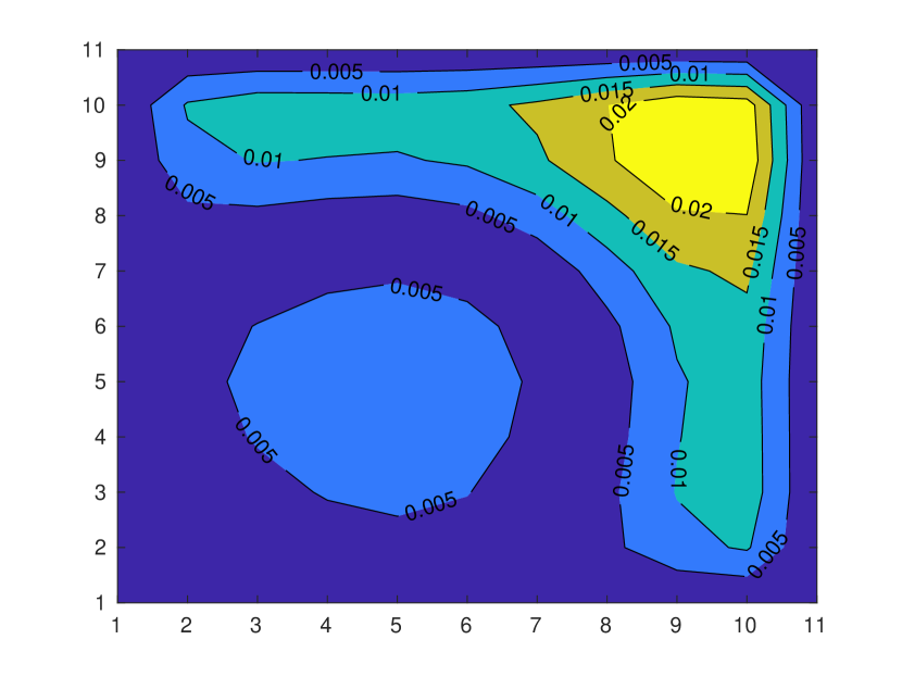
(a) Percentage error for 11$\times$11 congregated grid.

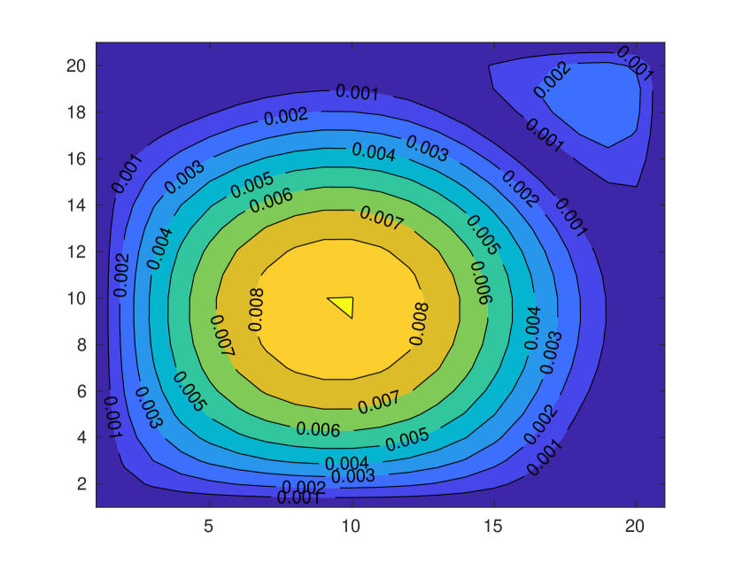
(b) Percentage error for 21$\times$21 congregated grid.

Figure 4: Contour plots of the percentage erros of the patch dynamics solutions with congregated grids 11$\times$11, $Nt=2000$ and 21$\times$21, $Nt=8500$ at time $t=1$ are shown here, with $\lambda=0.1$ in both of the solutions.

In Figure 4, a comparison is made between the percentage errors of two solutions with grids 11$\times$11, $Nt=2000$ and grid 21$\times$21, $Nt=8500$ respectively. In both cases, $\lambda=0.1$ is considered, and all other parameters are kept the same as previous. In Figure 4(a), an excellent accuracy is achieved, but a little error can be noticed in the high gradient region due to fewer macro grids. However, in Figure 4(b), better accuracy can be noticed in the high gradient region due to more clustered grids. However, overall, a significant accuracy is achieved in both of the solutions.

Grid Independence of the CDR equation with constant diffusivity in stretched domain:

Let, $T_{n\times m}$ and $T_{2n\times 2m}$ be the patch dynamics solutions with respect to the $(n+1)\times(m+1)$ and $(2n+1)\times(2m+1)$ grids respectively at a certain time. The rate of change of the above two solutions is $\left|\frac{|T_{(2n+1)\times(2m+1)}-T_{(n+1)\times(m+1)}|}{T_{(2n+1)\times(2m+1)}}\right|\times 100\%$, at a fixed time $t$.

To check the grid independence of the problem (21), the coarser grid $11\times 11$, $Nt=2000$ and the finer grid $21\times 21$, $Nt=8500$ are considered. The stretching factor is $\lambda=0.1$, and all other parameters are kept fixed in both solutions as contemplated in the previous. The maximum rate of change between the coarser and finer grid solutions is 0.0234% over the whole domain [0, 1]$\times$[0, 1] and within full time [0, 1]. If the maximum percentage error between the coarser and finer grid solutions is less than 0.1%, it is generally considered to be grid independent [32]. So the patch dynamics solution with the grid resolution $21\times 21$, $Nt=8500$ is considered grid independent.

CDR equation with variable diffusivity: A class of materials called Functionally Graded Materials (FGMs), which was invented by Niino et al. [33] in 1984 that could withstand extreme temperature gradients. In general, FGMs can be divided into three categories: gradient composition, gradient porosity and gradient microstructure, where the microstructure can be found in the articles [34, 35]. Looking into the micro-structure of the FGMs, the temperature distribution is solved in a large domain over a long time using micro-simulations in small patches in the following problem. To determine the temperature of the FGMs in a large domain over a long time, the next problem is selected. This problem considers the temperature distribution informations of the microstructure, which is taken care by the micro-simulations in the patch dynamics scheme. To investigate how the patch dynamics scheme adapts to CDR problems in functionally graded media, a model with variable velocity and diffusivity is considered. We assume the thermal diffusivity varies with the horizontal distance, which is $D_{x}=D_{y}=1+x$, convective velocities are $v_{x}=10x$, $v_{y}=10y$ and the source term is $S(x,y,t)=(8x+10y-1)e^{x+y+t}$ in (21). In the macroscopic domain, initial and boundary conditions are the same as in the problem (21). This physical problem has an exact solution given by (22). The clustered grid is used in the high gradient region by the transformation (23) to get a better accuracy. The grids, as well as the patches in the physical domain and in the computational domain may be taken similar as in the Figure 3.

	Maximum percentage errors
$\lambda$	$11\times 11,Nt=2000$	$16\times 16,Nt=5500$
0	0.0530	0.0185
0.1	0.0102	0.0086
0.2	0.0667	0.0322
0.3	0.1215	0.0553
0.4	0.1740	0.0779
0.5	0.2244	0.1000

Table 3: Maximum percentage errors in the patch dynamics solution for different stretching ratio $\lambda$ and for different resolutions.

Similarly, in the variable diffusivity problem, it can be observed that the best possible solution is obtained for the stretched grid with stretching parameter $\lambda=0.1$. In Figure 5, contour plots of the percentage errors of the patch dynamics solutions for congregated grids $11\times 11$ and $21\times 21$ are shown at the final time $t=1$ and with $\lambda=0.1$ in both the solutions.

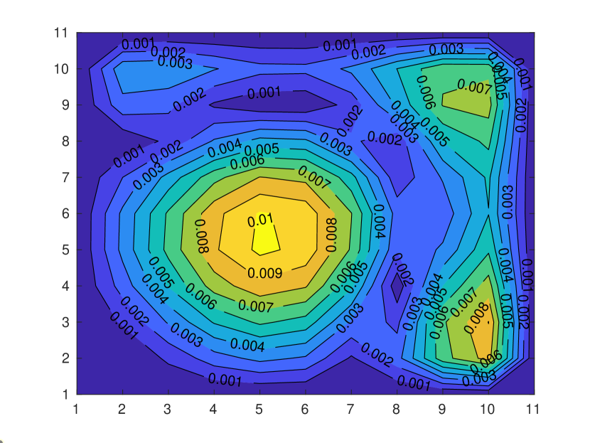
(a) Percentage error for 11$\times$11 congregated grid.

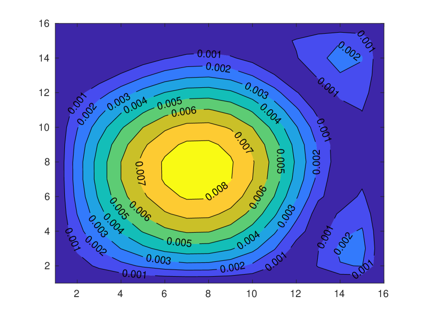
(b) Percentage error for 21$\times$21 congregated grid.

Figure 5: Contour plots of the percentage erros of the patch dynamics solutions with congregated grids 11$\times$11, $Nt=2000$ and 21$\times$21, $Nt=8500$ at time $t=1$ are shown here, with $\lambda=0.1$ in both of the solutions.

The grid independence is checked for variable diffusivity problems, with a coarser grid $11\times 11$, $Nt=2000$ and finer grid $21\times 21$, $Nt=8500$. The stretching factor in both cases is $\lambda=0.1$, and all other parameters are kept the same as considered in the previous. The maximum rate of change between the coarser and the finer grid solutions is 0.0093% over the whole domain $[0,1]^{2}$ and within full-time [0, 1]. Hence, the patch dynamics solution with the grid resolution $21\times 21$, $Nt=8500$ is grid independent.

5.2 A problem on non-axisymmetric diffusion in an annulus region

Various fields, like mass transfer in chemical engineering and biology, heat transfer in nuclear reactors, etc., can be modelled by the two-dimensional diffusion equations. In biology, multiscale techniques are developed to model the mass transport phenomenons in biological tissues [36, 37, 38], where the microscopic problem is a 2D diffusion equation. An annular structure is often found in the membranes of living organisms. In cellular biology, an annulus region can be considered to describe the diffusion of molecules or ions through the lipid bilayer of cell organelles or membranes [39, 40]. Several physiological processes depend on this, including the transport of nutrients and the removal of waste [41, 42]. To solve these equations, a patch dynamics scheme has been proposed in this paper.

$\underline{\textbf{Physical Problem:}}$

$$\begin{cases}\text{PDE:}\hskip 4.26773ptu_{t}=D(\frac{\partial^{2}u}{\partial x^{2}}+\frac{\partial^{2}u}{\partial y^{2}}),\hskip 7.11317pt\text{in}\hskip 7.11317pt\Omega_{p}\hskip 7.11317pt\text{and}\hskip 7.11317ptt\in(0,1],\\ \hskip 11.38092pt\text{IC:}\hskip 4.26773ptu(x,y,0)=(\sqrt{x^{2}+y^{2}}-1)(2-\sqrt{x^{2}+y^{2}})\sin(\arctan(\frac{y}{x})),\hskip 7.11317pt\text{in}\hskip 7.11317pt\overline{\Omega}_{p},\\ \hskip 3.69899pt\text{BCs:}\hskip 4.26773ptu(x,y,t)=0,\hskip 7.11317pt\text{along inner most circle}\hskip 7.11317pt\Gamma_{in}=\left\{(x,y):x^{2}+y^{2}=1^{2}\right\},\\ \hskip 31.2982ptu(x,y,t)=0,\hskip 7.11317pt$\text{along outer most circle}$\hskip 7.11317pt\Gamma_{out}=\left\{(x,y):x^{2}+y^{2}=2^{2}\right\}\hskip 7.11317pt\text{and}\hskip 7.11317ptt\in[0,1].\end{cases}$$ (25)

To do the computation, a transform between the polar and Cartesian grids is taken, as shown in figure 6 as follows,

$$x=r\cos(\theta),\hskip 7.11317pty=r\sin(\theta),\hskip 7.11317pt\text{or}\hskip 7.11317ptr=\sqrt{x^{2}+y^{2}},\hskip 7.11317pt\theta=\arctan\left(\frac{y}{x}\right).$$ (26)

Figure 6: Left: Physical domain & Right: Computational domain

$\underline{\textbf{Computational Problem:}}$

$$\begin{cases}\text{PDE:}\hskip 7.11317ptu_{t}=D(\frac{\partial^{2}u}{\partial r^{2}}+\frac{1}{r}\frac{\partial u}{\partial r}+\frac{1}{r^{2}}\frac{\partial^{2}u}{\partial\theta^{2}}),\hskip 7.11317pt\text{in}\hskip 7.11317pt\Omega_{c}=(0,2\pi)\times(1,2)\hskip 7.11317pt\text{and}\hskip 7.11317ptt\in(0,1],\\ \hskip 11.38092pt\text{IC:}\hskip 7.11317ptu(\theta,r,t=0)=(r-1)(2-r)\sin(\theta),\hskip 7.11317pt\text{in}\hskip 7.11317pt\overline{\Omega}_{c},\\ \hskip 2.84544pt\text{BCs:}\hskip 7.11317ptu(\theta,r=1,t)=0,\hskip 7.11317ptu(\theta,r=2,t)=0,\hskip 7.11317ptu(\theta=0,r,t)=u(\theta=2\pi,r,t),\text{and}\\ \hskip 25.6073pt\hskip 7.11317pt\frac{\partial u}{\partial\theta}(\theta=0,r,t)=\frac{\partial u}{\partial\theta}(\theta=2\pi,r,t),\hskip 7.11317ptt\in[0,1].\end{cases}$$ (27)

The analytical solution of the computational problem is given by

$$u(r,\theta,t)=\frac{\pi^{2}}{2}\sum_{m=1}^{\infty}\left[\int_{1}^{2}\xi(\xi-1)(2-\xi)Z_{1}(\mu_{1,m}\xi)d\xi\right]B_{1,m}Z_{1}(\mu_{1,m}r)\sin\theta\exp(-\mu_{1,m}^{2}t),$$ (28)

where $B_{1,m}=\frac{\mu_{1,m}^{2}J_{1}^{2}(2\mu_{1,m})}{J_{1}^{2}(\mu_{1,m})-J_{1}^{2}(2\mu_{1,m})}$, $Z_{1}(\mu_{1,m}r)=J_{1}(\mu_{1,m})Y_{1}(\mu_{1,m}r)-Y_{1}(\mu_{1,m})J_{1}(\mu_{1,m}r)$, $J_{1}$ and $Y_{1}$ are the Bessel’s functions of first kind and second kind respectively. $\mu_{1,m}$ are the positive roots of the transcendental equation $J_{1}(\mu)Y_{1}(2\mu)-Y_{1}(\mu)J_{1}(2\mu)=0$.

	Maximum percentage errors
($Nx,Ny,Nt$)	$t=0.25$	$t=0.5$	$t=0.75$	$t=1$
(16, 10, 500)	0.6824	1.3115	1.9362	2.5569
(24, 15, 1200)	0.2582	0.4961	0.7333	0.9700
(32, 20, 2000)	0.2064	0.4042	0.6014	0.7983
(40, 25, 3200)	0.1387	0.2745	0.4100	0.5454
(48, 30, 4500)	0.1169	0.2341	0.3510	0.4679
(56, 35, 6200)	0.0952	0.1927	0.2900	0.3872
(64, 40, 8000)	0.0854	0.1743	0.2631	0.3518

Table 4: Percentage errors in the patch dynamics solution of the problem (25) for different resolutions of the macroscopic domain and at different times.

The results are presented here after the computation on different macroscopic grid resolutions in Table 4, Figures 7 and 8 show the convergence of the patch dynamics scheme. In the computational domain, the uniform patch sizes are $h_{x}=h_{y}=0.001$ and $\tau=1e{-6}$. At the microscopic level, the patches are discretized with $nx=ny=20$ and time is discretized with $nt=1500$. The central difference scheme is used in both radial and azimuthal derivatives, and forward difference is used in the temporal derivative.

In Table 4, the maximum percentage errors of the patch dynamics solution of the problem (25) is shown with respect to the analytical solution (28) for different resolutions and at times $t=0.25,t=0.5,t=0.75$ and $t=1$. The maximum percentage error over the whole annulus domain and within the full-time interval [0, 1] equals the maximum percentage error at the final time $t=1$. From the above table, it can be observed that the patch dynamics solutions are in good agreement with the analytical solution.

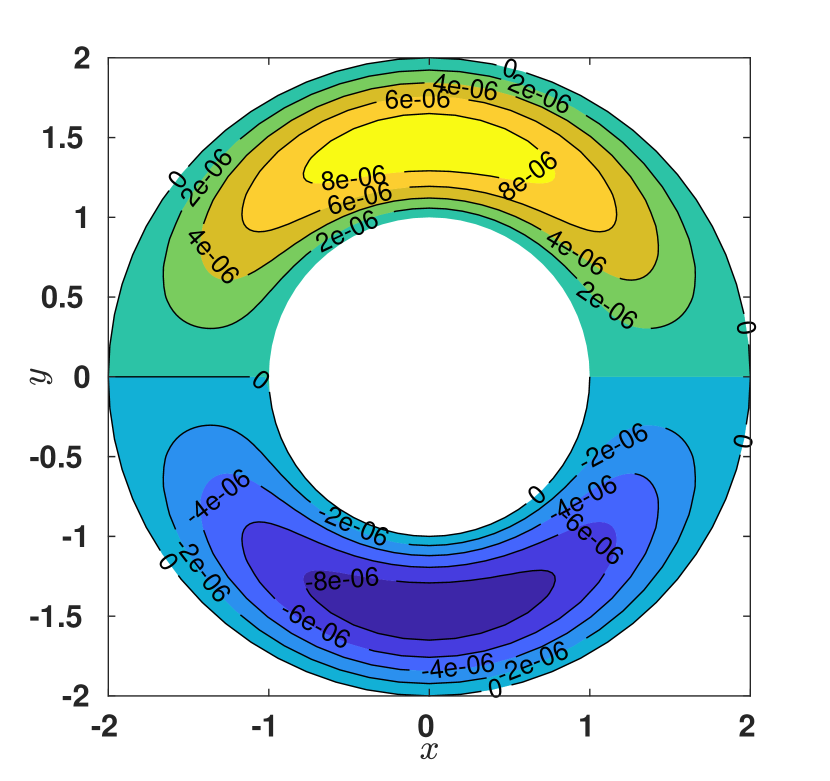
(a) Analytical solution

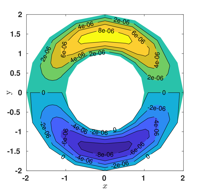
(b) Grids 17$\times$11

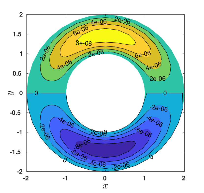
(c) Grids 33$\times$21

(d) Grids 65$\times$41

Figure 7: Analytical solution and patch dynamics solutions for different grid resolutions at final time $t=1$.

Figure 7 displays solutions analytical and patch dynamics contours. One can hardly distinguish the numerical solutions from the exact solution. As Figure 7(b) has fewer grids, the curved contour parts do not look so smooth.

In Figure 8, the surface plots of the absolute errors in the patch dynamics solutions are shown on different grid sizes $17\times 11$, $33\times 21$ and $65\times 41$ at time $t=1$ for which the maximum percentage errors are 2.34623$\times 10^{-7}$, 7.30332$\times 10^{-8}$ and 3.22512$\times 10^{-8}$ respectively. From all the previous results of the problem (25), it can be observed that the patch dynamics scheme can handle periodic boundary conditions at the macroscopic level in the computational domain. Also, using a body-fitted curvilinear coordinate system, one can find the patch dynamics solution in the non-rectangular domain.

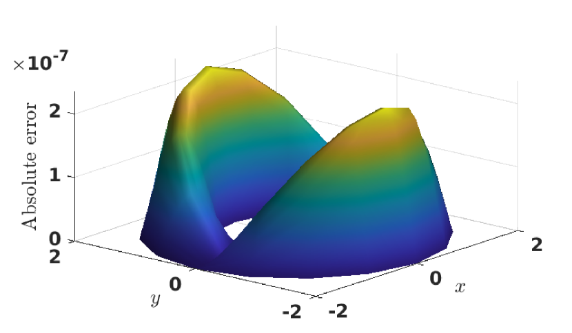
(a) Grids 17$\times$11

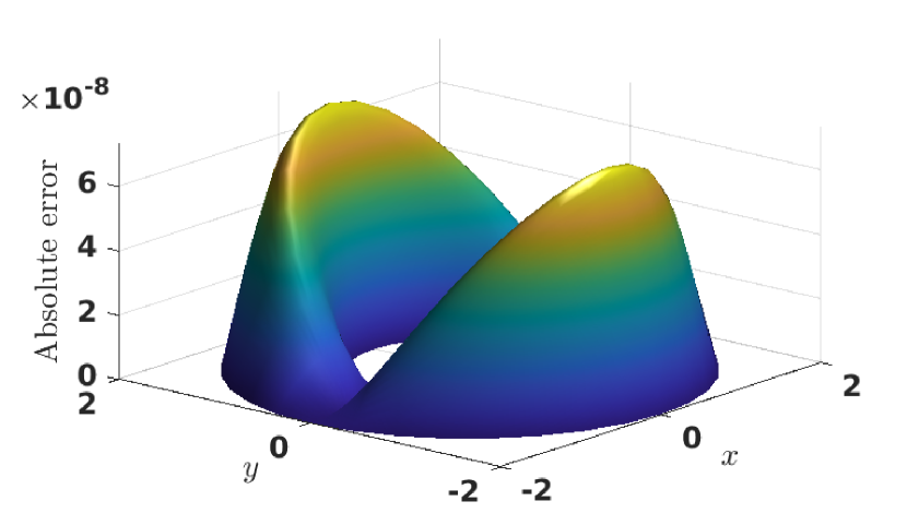
(b) Grids 33$\times$21

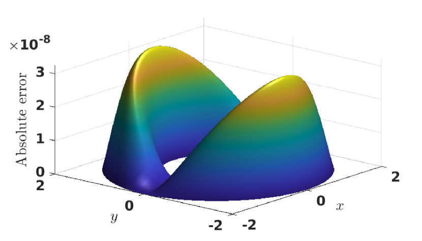
(c) Grids 65$\times$41

Figure 8: Absolute error in the patch dynamics solutions at final time $t=1$.

6 Conclusion

The Patch dynamics schemes, have so far been developed, are specifically on rectangular domains considering uniform spatial grids and uniform patch sizes. However, considering the complexities arising from both physical and geometrical aspects of the various problems, it is evident that grids may not always be uniform, and domains may not necessarily be rectangular. An explicit patch dynamics scheme is proposed in this study to address the challenges posed by two-dimensional evolution equations on non-rectangular domains with non-uniform grids in order to determine the system level behavior in large domains over a long time. This scheme is applied to linear unsteady convection-diffusion-reaction (CDR) problems. The shape and size of each patch are determined based on the physical and geometrical complexities of the problem, and generalized curvilinear coordinates are employed to handle such complexities. Based on such complexities, two different types of numerical problems are chosen for validation. In the first problem, a convection-dominated two-dimensional CDR equation is considered over a rectangular domain with high gradients at the right and top boundaries, and a stretched grid is employed in such regions. Non-homogeneous Dirichlet boundary conditions are considered, exhibiting exponential growth along the $x$- and $y$- directions. In the first and second parts of the problem, constant and variable diffusivities are considered, and their solutions are verified with the analytical solution and some existing numerical solutions. The grid independence of both patch dynamics solutions is demonstrated on $21\times 21$ grid over $Nt=8500$ time steps. In the second one, a 2D unsteady non-axisymmetric diffusion problem is solved in an annulus using the body-fitted curvilinear coordinate system. There is an excellent agreement between the solutions obtained for the proposed scheme and existing findings.

This study leads to the following conclusions:

1. A methodical representation of the two-dimensional patch dynamics scheme is proposed on general evolution equations on the generalized curvilinear coordinate system in a two-dimensional domain.

2. The patch dynamics scheme is tailored to solve multiscale problems on non-uniform grids and non-rectangular domains, accommodating non-uniform and non-rectangular patch configurations within the physical domain. So, this method can be applied to general problems. In this article, the method is applied on linear unsteady CDR problems.

3. Stretched grids with a stretching ratio, $\lambda=0.1$ provide a better accuracy compared to unstretched grids (or uniform grids where $\lambda$=0) and other stretching ratios ($\lambda\neq 0.1$). Stretched grids notably reduce errors substantially in the high-gradient regions.

4. The proposed patch dynamics scheme can efficiently handle a non-axisymmetric diffusion problem in an annulus region with periodic and Dirichlet boundary conditions.

References

- [1] Richard Car and Mark Parrinello. Unified approach for molecular dynamics and density-functional theory. Physical review letters, 55(22):2471, 1985.
- [2] Francois Coron and Benoit Perthame. Numerical passage from kinetic to fluid equations. SIAM Journal on Numerical Analysis, 28(1):26–42, 1991.
- [3] Ellad B Tadmor, Michael Ortiz, and Rob Phillips. Quasicontinuum analysis of defects in solids. Philosophical magazine A, 73(6):1529–1563, 1996.
- [4] J Knap and M Ortiz. An analysis of the quasicontinuum method. Journal of the Mechanics and Physics of Solids, 49(9):1899–1923, 2001.
- [5] Davi R Ortega, Chen Yang, Peter Ames, Jerome Baudry, John S Parkinson, and Igor B Zhulin. A phenylalanine rotameric switch for signal-state control in bacterial chemoreceptors. Nature communications, 4(1):2881, 2013.
- [6] Kenta Kiuchi, Koutarou Kyutoku, Yuichiro Sekiguchi, Masaru Shibata, and Tomohide Wada. High resolution numerical relativity simulations for the merger of binary magnetized neutron stars. Physical Review D, 90(4):041502, 2014.
- [7] Trung Dac Nguyen, Jan-Michael Y Carrillo, Michael A Matheson, and W Michael Brown. Rupture mechanism of liquid crystal thin films realized by large-scale molecular simulations. Nanoscale, 6(6):3083–3096, 2014.
- [8] Ioannis G Kevrekidis, C William Gear, James M Hyman, Panagiotis G Kevrekidis, Olof Runborg, Constantinos Theodoropoulos, et al. Equation-free, coarse-grained multiscale computation: enabling microscopic simulators to perform system-level analysis. Commun. Math. Sci, 1(4):715–762, 2003.
- [9] C William Gear and Ioannis G Kevrekidis. Projective methods for stiff differential equations: problems with gaps in their eigenvalue spectrum. SIAM Journal on Scientific Computing, 24(4):1091–1106, 2003.
- [10] CW Gear and Ioannis G Kevrekidis. Telescopic projective methods for parabolic differential equations. Journal of Computational Physics, 187(1):95–109, 2003.
- [11] Giovanni Samaey, Dirk Roose, and Ioannis G Kevrekidis. The gap-tooth scheme for homogenization problems. Multiscale Modeling & Simulation, 4(1):278–306, 2005.
- [12] Giovanni Samaey, Ioannis G Kevrekidis, and Dirk Roose. Patch dynamics with buffers for homogenization problems. Journal of Computational Physics, 213(1):264–287, 2006.
- [13] Hassan Arbabi, Judith E Bunder, Giovanni Samaey, Anthony J Roberts, and Ioannis G Kevrekidis. Linking machine learning with multiscale numerics: data-driven discovery of homogenized equations. Jom, 72(12):4444–4457, 2020.
- [14] Ping Liu, Giovanni Samaey, C William Gear, and Ioannis G Kevrekidis. On the acceleration of spatially distributed agent-based computations: A patch dynamics scheme. Applied Numerical Mathematics, 92:54–69, 2015.
- [15] G Samaey, AJ Roberts, and IG Kevrekidis. Equation-free computation: An overview of patch dynamics. Multiscale methods: bridging the scales in science and engineering, page 216, 2009.
- [16] Steven L Lee and C William Gear. Second-order accurate projective integrators for multiscale problems. Journal of Computational and Applied Mathematics, 201(1):258–274, 2007.
- [17] John Maclean and Georg A Gottwald. On convergence of higher order schemes for the projective integration method for stiff ordinary differential equations. Journal of Computational and Applied Mathematics, 288:44–69, 2015.
- [18] C William Gear, Ju Li, and Ioannis G Kevrekidis. The gap-tooth method in particle simulations. Physics Letters A, 316(3-4):190–195, 2003.
- [19] Ioannis G Kevrekidis and Giovanni Samaey. Equation-free multiscale computation: Algorithms and applications. Annual review of physical chemistry, 60:321–344, 2009.
- [20] James M Hyman. Patch dynamics for multiscale problems. Computing in science & engineering, 7(3):47–53, 2005.
- [21] John Maclean, JE Bunder, and Anthony J Roberts. A toolbox of equation-free functions in matlab/octave for efficient system level simulation. Numerical Algorithms, 87(4):1729–1748, 2021.
- [22] Ju Li, Panayotis G Kevrekidis, C William Gear, and Ioannis G Kevrekidis. Deciding the nature of the coarse equation through microscopic simulations: The baby-bathwater scheme. SIAM review, 49(3):469–487, 2007.
- [23] AJ Roberts, Tony MacKenzie, and Judith E Bunder. A dynamical systems approach to simulating macroscale spatial dynamics in multiple dimensions. Journal of Engineering Mathematics, 86(1):175–207, 2014.
- [24] JE Bunder, Anthony J Roberts, and Ioannis G Kevrekidis. Good coupling for the multiscale patch scheme on systems with microscale heterogeneity. Journal of Computational Physics, 337:154–174, 2017.
- [25] JE Bunder, Ioannis G Kevrekidis, and Anthony J Roberts. Equation-free patch scheme for efficient computational homogenisation via self-adjoint coupling. Numerische Mathematik, 149(2):229–272, 2021.
- [26] Swapan K Pandit, Jiten C Kalita, and DC Dalal. A transient higher order compact scheme for incompressible viscous flows on geometries beyond rectangular. Journal of Computational Physics, 225(1):1100–1124, 2007.
- [27] Swapan K Pandit, Jiten C Kalita, and DC Dalal. A fourth-order accurate compact scheme for the solution of steady navier–stokes equations on non-uniform grids. Computers & fluids, 37(2):121–134, 2008.
- [28] Rajendra K Ray and Jiten C Kalita. A transformation-free hoc scheme for incompressible viscous flows on nonuniform polar grids. International journal for numerical methods in fluids, 62(6):683–708, 2010.
- [29] Arthur Piquet, Boubakr Zebiri, Abdellah Hadjadj, and Mostafa Safdari Shadloo. A parallel high-order compressible flows solver with domain decomposition method in the generalized curvilinear coordinates system. International Journal of Numerical Methods for Heat & Fluid Flow, 30(1):2–38, 2020.
- [30] Yuanyuan Zhao, Mei Huang, Xiaoping Ouyang, Jun Luo, Yongqing Shen, and Fang Bao. A half boundary method for two dimensional unsteady convection–diffusion equations. Engineering Analysis with Boundary Elements, 135:322–336, 2022.
- [31] Lixin Ge and Jun Zhang. High accuracy iterative solution of convection diffusion equation with boundary layers on nonuniform grids. Journal of Computational Physics, 171(2):560–578, 2001.
- [32] Sandip Mazumder. Numerical methods for partial differential equations: finite difference and finite volume methods. Academic Press, 2015.
- [33] M Niino, T Hirai, and R Watanabe. Functionally gradient materials. in pursuit of super heat resisting materials for spacecraft. J. Jpn. Soc. Compos. Mater, 13:257–264, 1987.
- [34] Majid Mohammadi, Masoud Rajabi, and Majid Ghadiri. Functionally graded materials (fgms): A review of classifications, fabrication methods and their applications. Processing and Application of Ceramics, 15(4):319–343, 2021.
- [35] Dalia Mahmoud and Mohamed A Elbestawi. Lattice structures and functionally graded materials applications in additive manufacturing of orthopedic implants: a review. Journal of Manufacturing and Materials Processing, 1(2):13, 2017.
- [36] KS Yadav and DC Dalal. The heterogeneous multiscale method to study particle size and partitioning effects in drug delivery. Computers & Mathematics with Applications, 92:134–148, 2021.
- [37] Mohammad Aminul Islam, Sutapa Barua, and Dipak Barua. A multiscale modeling study of particle size effects on the tissue penetration efficacy of drug-delivery nanoparticles. BMC Systems Biology, 11:1–13, 2017.
- [38] Di Su, Ronghui Ma, Maher Salloum, and Liang Zhu. Multi-scale study of nanoparticle transport and deposition in tissues during an injection process. Medical & biological engineering & computing, 48:853–863, 2010.
- [39] DA Haydon and SB Hladky. Ion transport across thin lipid membranes: a critical discussion of mechanisms in selected systems. Quarterly reviews of biophysics, 5(2):187–282, 1972.
- [40] Rainer A Böckmann, Agnieszka Hac, Thomas Heimburg, and Helmut Grubmüller. Effect of sodium chloride on a lipid bilayer. Biophysical journal, 85(3):1647–1655, 2003.
- [41] William M Pardridge. Transport of nutrients and hormones through the blood-brain barrier. Diabetologia, 20:246–254, 1981.
- [42] Diganta Bhusan Das. Multiscale simulation of nutrient transport in hollow fibre membrane bioreactor for growing bone tissue: sub-cellular scale and beyond. Chemical engineering science, 62(13):3627–3639, 2007.