Effect of injection conditions on the non-linear behavior of the ECDI and related turbulent transport

Abstract

The electron-cyclotron drift instability (ECDI) has been proposed as one of the main actors behind the anomalous transport of electrons in Hall thruster devices. In this work, we revisit the theory and perform two-dimensional PIC simulations under several conditions to analyze the non-linear behavior and the induced transport under several boundary conditions. Simulation results with fully-periodic boundaries and conditions faithful to the linear theory show the growth of ECDI modes, ion-wave trapping vortexes and agree with the existing literature in early times. In the long term, however, we observe very mild oscillations and null anomalous current. The evolution towards this new equilibrium is coherent to what can be expected from energy conservation. The quenching of the oscillations seem to be highly related with the distortion of ion-trapping vortexes in phase space after a long-term interaction of ion particles with the electrostatic wave. This result suggests that sustained oscillations and turbulent current could benefit from the renewal of ions by, e.g., removing and injecting particles through axial boundaries instead of applying periodicity. This second type of simulations shows that injection conditions highly impact the late simulation behavior of ECDI oscillations, where we identify several regimes depending on the value of the ion residence time compared to the characteristic saturation time in the fully periodic case. The intermediate regime, where these two times are close, is the only one providing sustained oscillations and electron transport and seems to be the relevant one in Hall devices.

I Introduction

The problem of anomalous electron cross-field transport remains as one of big open challenges for the community of $\bm{E}\times\bm{B}$ plasmas. In the field of plasma propulsion, this problem has been mainly studied in the context of Hall-thruster discharges and represent one big obstacle on the way towards to predictive efficient numerical models. The large drift of electrons in the azimuthal direction of the Hall thruster is a source of several families of azimuthal oscillations that are potential candidates to explain the anomalous transport and have been observed experimentally [1, 2, 3, 4, 5, 6]. The classical explanation [7] for the impact of oscillations on transport relies on the correlation of oscillations in density and electric field in the $\bm{E}\times\bm{B}$ direction under the presence of a magnetic field.

The amount of articles devoted to the analysis of instabilities and turbulence in Hall thrusters is extensive. With a macroscopic description for ions and electrons, some of the authors of this article have conducted global [8] and local [9] linear stability analyses. In these references two-stream, drift-gradient and drift-dissipative instabilities are discussed. Similar recent studies by other authors are [10, 11, 12, 13, 14].

When using a kinetic formulation for the electrons, the analytical studies of instabilities are usually limited to a homogeneous and collisionless plasma. For the conditions of a Hall thruster, where electrons are magnetized but ions are not, the dispersion relation of the electron cyclotron drift instability (ECDI) is obtained[15, 16]. This classical instability have been revisited, during the last two decades, by several authors [17, 18, 19, 20, 21], in the context of Hall thrusters. Also from the point of view of kinetic simulations [17, 22, 23, 24, 25, 26] and experiments [27, 4, 5, 6].

Kinetic models aimed to analyze electron turbulence and turbulent transport in the plane perpendicular to the applied magnetic field $\bm{B}_{0}$ can be classified in 1D azimuthal[25, 22, 26] and 2D axial-azimuthal [17, 23, 24]. The latter case has been the subject of a recent benchmark by several groups [28]. Many 2D simulations include a number of phenomena that makes challenging to compare the results with the ECDI linear theory; such as, inhomogeneous magnetic field, collisions, ionization or electrical connection between anode and cathode. The 1D-azimuthal simulations are closer to the linear theory of the ECDI but some of them still add effects that are not considered in the dispersion relation, such as refreshing of particle velocities or collisions. Moreover, the 1D simulation results reported in the literature have been seen to be sensitive to the axial treatment of particles; observing a sustained saturated state only when using a virtual axial dimension and particle velocities are refreshed after leaving the domain axially [22, 26]. If particle are not refreshed an unbounded growth of oscillations and heating are seen [25, 29].

In section II, we revisit the main results from the classical dispersion relation of the ECDI theory. A recently developed in-house two-dimensional PIC code is introduced in section III and used to analyze the nonlinear evolution of the ECDI under several conditions. In every case, a 2D domain perpendicular to $\bm{B}_{0}$ is considered; which we will refer to as the axial-azimuthal plane, making the analogy with a Hall discharge geometry. Initially we consider a fully periodic domain and simulate under the assumptions of the classical ECDI theory. These results can be compared with the existing literature [25, 22, 26] on 1D azimuthal simulations of the classical ECDI, but open the possibility to the growth of modes with an axial component. Similar results to those shown elsewhere are found during early simulation times; but our long-term behavior shows no oscillation capable of driving an turbulent electron transport, which disagrees with the literature. We try to give an explanation from an energy conservation perspective.

Periodic results establish a clear relation between ion behavior and the existence of electron transport in the long term, what suggests that renewal of ion particles could help to develop sustained ECDI oscillations and axial transport. This motivate us to replace axial boundary conditions from periodic to removal/injection of particles, which mimics the generation and loss of particles in a finite plasma such as the Hall discharge. Results are shown in section IV, where we are able to establish a clear relation between the ion velocity (related with the residence time) and the long-term behavior of short-wavelength oscillations and transport in the plasma.

II The classical ECDI: linear analysis

We attempt to study the stability of an homogeneous, collisionless plasma at equilibrium subjected to mutually perpendicular magnetic $\bm{B}_{0}=B_{0}\bm{1}_{x}$ and electric $\bm{E}_{0}=E_{0}\bm{1}_{z}$ fields. Throughout the article subindex ‘0’ and ‘1’ stand for equilibrium and perturbed conditions. Consistent with Hall thruster discharges: the strength of the stationary magnetic field keeps electrons well-magnetized and ions unmagnetized, and the plasma currents are low enough to neglect the contribution of the self-induced magnetic field $\bm{B}_{1}$. At equilibrium, electrons have a drifted-Maxwellian velocity distribution function (VDF) with density $n_{0}$, temperature $T_{e0}$, and an $\bm{E}_{0}\times\bm{B}_{0}$ drift velocity $\bm{u}_{e0}=u_{ye0}\bm{1}_{y}$, $u_{ye0}=E_{0}/B_{0}$. Equilibrium ions are assumed cold, have a density $n_{0}$, and move with a constant velocity $\bm{u}_{i0}=u_{zi0}\bm{1}_{z}$, parallel to $\bm{E}_{0}$. This homogeneous equilibrium disregards the electrostatic acceleration of ions due to $\bm{E}_{0}$. From analogy with a Hall-thruster geometry, let us refer throughout the article to the directions of $\bm{B}_{0}$, $\bm{E}_{0}$ and $\bm{E}_{0}\times\bm{B}_{0}$ as radial ($x$), axial ($z$) and azimuthal ($y$).

Next, we summarize the main aspects of the well-known linear stability analysis [15, 16, 18, 19, 20] From the linearly perturbed Vlasov equation, the relation between the electron density and the electric potential perturbations of wavevector $\bm{k}$ and complex frequency $\omega$, for propagation perpendicular to $\bm{B}_{0}$ (i.e., the component of $\bm{k}$ parallel to $\bm{B}_{0}$ is zero), is

$$\frac{n_{e1}}{n_{0}}=\Big{[}1-g(\omega_{e},b_{e};\omega_{ce})\Big{]}\frac{e\phi_{1}}{T_{e0}}$$ (1)

with

$$g(\omega_{e},b_{e};\omega_{ce})=\exp(-b_{e})\Big{[}I_{0}(b_{e})+2\sum_{m=1}^{\infty}\frac{\omega_{e}^{2}I_{m}(b_{e})}{\omega_{e}^{2}-m^{2}\omega_{ce}^{2}}\Big{]}.$$ (2)

In these equations $\bm{E}=-\nabla\phi$, $c_{e0}=\sqrt{T_{e0}/m_{e}}$ is the electron thermal velocity, $\omega_{ce}=eB_{0}/m_{e}$ is the cyclotron frequency, $b_{e}=k^{2}\rho_{e0}^{2}$, $\rho_{e0}=c_{e0}/\omega_{ce}$ is the electron Larmor radius, $\omega_{e}=\omega-k_{y}u_{ye0}$ is the electron Doppler-shifted frequency, $\bm{k}=k_{y}\bm{1}_{y}+k_{z}\bm{1}_{z}$, and $I_{m}$ are the modified Bessel functions of the first kind. According to equation (2), the perturbed electron response has resonances at the electron gyrofrequency and its harmonics, i.e. $\omega_{e}=m\omega_{ce}$.

Next, the density perturbations of cold ions follow

$$\frac{n_{i1}}{n_{0}}=\frac{k^{2}c_{s0}^{2}}{\omega_{i}^{2}}\frac{e\phi_{1}}{T_{e0}},$$ (3)

with $\omega_{i}=\omega-k_{z}u_{zi0}$ the ion Doppler-shifted frequency, and $c_{s0}=\sqrt{T_{e0}/m_{i}}$ the ion sound speed. Using Eqs. (1) and (3), together with the linearized Poisson equation, yields the two-dimensional dispersion relation

$$1+k^{2}\lambda_{D0}^{2}=\frac{k^{2}c_{s0}^{2}}{\omega_{i}^{2}}+g(\omega_{e},b_{e};\omega_{ce}).$$ (4)

This equation is solved for the complex frequencies $\omega=\omega_{r}+\text{i}\gamma$ with all other parameters fixed, including $\bm{k}$.

Type	Description and symbol	Value and units
Fundamental plasma parameters	Ion mass, $m_{i}$	1 u
	Electric field, $E_{0}$	$10^{4}$ V/m
	Magnetic field, $B_{0}$	200 G
	Plasma density, $n_{0}$	$10^{17}$ m-3
	Ion axial velocity, $u_{zi0}$	2.5 km/s
	Electron temperature, $T_{e0}$	6 eV
Derived plasma parameters	Electron azimuthal drift, $u_{ye0}$	500 km/s
	Electron thermal speed, $c_{e0}$	1027 km/s
	Sound speed, $c_{s0}$	23.97 km/s
	Debye length, $\lambda_{D0}$	57.58 $\mu$m
	Electron azimuthal-drift gyroradius, $\ell_{e0}$	142.1 $\mu$m
	Electron Larmor radius, $\rho_{e0}$	292.0 $\mu$m
	Electron plasma frequency, $\omega_{pe0}$	2.839 GHz
	Electron gyrofrequency, $\omega_{ce}$	0.5600 GHz
	Ion plasma frequency, $\omega_{pi0}$	66.26 MHz
	Lower-hybrid frequency, $\omega_{lh}$	13.07 MHz
Fundamental numerical parameters	Azimuthal domain length, $L_{y}$	5.359 mm
	Axial domain length, $L_{z}$	2.679 mm
	Number of azimuthal celss, $N_{y}$	100
	Number of axial cells, $N_{z}$	50
	Number of particles per cell, $N_{\textmd{ppc}}$	200
	Time steps, $\Delta t$	$5\times 10^{-12}$ s
	Number of time steps, $N_{t}$	$6\times 10^{5}$
	Number of time steps between print-outs, $N_{\textmd{print}}$	1000
Derived numerical parameters	Azimuthal cell size, $\Delta y$	53.59 $\mu$m
	Axial cell size, $\Delta z$	53.59 $\mu$m

Table 1: Physical and numerical parameters of the reference simulation case. The subscript ‘0’ stands for initial equilibrium conditions. Derived parameter values are included for completeness but can be computed from fundamental ones.

The solutions of the dispersion relation are pairs of modes of three types [16]. First, there is a pair of ion-acoustic modes with $g\ll k^{2}c_{s0}^{2}/\omega_{i}$ and real-valued frequencies $\omega_{i}=\pm\omega_{\textmd{IA}}$; being

$$\omega_{\textmd{IA}}=\frac{kc_{s0}}{\sqrt{1+k^{2}\lambda_{D0}^{2}}},$$ (5)

which include a non-neutral term in the denominator that corrects the quasineutral linear relation $\omega_{i}=\pm kc_{s0}$. Second, there are electron Bernstein waves [30], with $g\gg k^{2}c_{s0}^{2}/\omega_{i}$ and real-valued frequencies too, close to the resonances $\omega_{e}=m\omega_{ce}$. Third, when $g\sim k^{2}c_{s0}^{2}/\omega_{i}$, Bernstein waves become coupled with the ion acoustic modes, yielding one of them the modified ion acoustic (MIA) pair with frequencies

$$\omega_{i}=\pm\frac{kc_{s0}}{\sqrt{1+k^{2}\lambda_{D0}^{2}-g(\omega_{e})}}.$$ (6)

For $g>1+k^{2}\lambda_{D0}^{2}$, one of MIA modes is unstable leading to the so called ECDI. Since $g$ changes from $-\infty$ to $+\infty$ when crossing the resonance $\omega_{e}=m\omega_{ce}$ with $\omega_{e}$ increasing, the MIA mode starts becoming unstable at $\omega_{e}=(m\omega_{ce})^{+}$ and becomes stable before reaching the $(m+1)$ resonance [18, 19, 20].

Figure 1 depicts, for the equilibrium solution of Table 1, the complex frequency of the purely-azimuthal (i.e. $\bm{k}=k_{y}\bm{1}_{y}$) MIA mode, and shows the growth rate of the ECDI linked to each $m\omega_{ce}$; as a function of $k_{y}\ell_{e0}$, being $\ell_{e0}=u_{ye0}/\omega_{ce}$ the azimuthal-drift gyroradius. The ion-acoustic frequency $\omega_{\textmd{IA}}$ is also plotted for comparison with the MIA mode. The same equilibrium solution will be used in the kinetic simulations of the coming sections. For $k_{y}>0$, the unstable mode has $\omega_{r}>0$, meaning propagation in the $\bm{E}_{0}\times\bm{B}_{0}$ direction. Due to symmetry, for $k_{y}<0$, the unstable mode has $\omega_{r}<0$ (i.e., moving again along $\bm{E}_{0}\times\bm{B}_{0}$) and same $\gamma$. In the purely azimuthal ECDI, one has $\omega\sim k_{y}c_{s}\ll\omega_{e}\simeq-k_{y}u_{ye0}\approx-m\omega_{ce}$. Therefore, the electron (Bernstein-type) response is quasi-steady and defines mostly the wavelength of the ECDI. Regarding nonneutral effects the MIA is quasineutral as long as $k_{y}^{2}\lambda_{D0}^{2}\ll 1$, i.e.

$$\dfrac{\lambda_{D0}}{\rho_{e}}\ll\dfrac{u_{y_{e0}}}{mc_{e0}}$$ (7)

and non-neutral effects tend to reduce the complex frequency. This effect is very clearly seen in the curve $\omega_{\textmd{IA}}$ in figure 1(a), that shows frequencies lowered with respect to a quasineutral ion-acoustic linear relation. The comparison of the MIA and ion-acoustic frequencies demonstrates that they follow the same trend but with significant deviations coming from the coupling with the Bernstein terms.

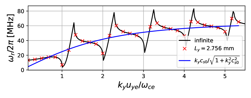
(a)

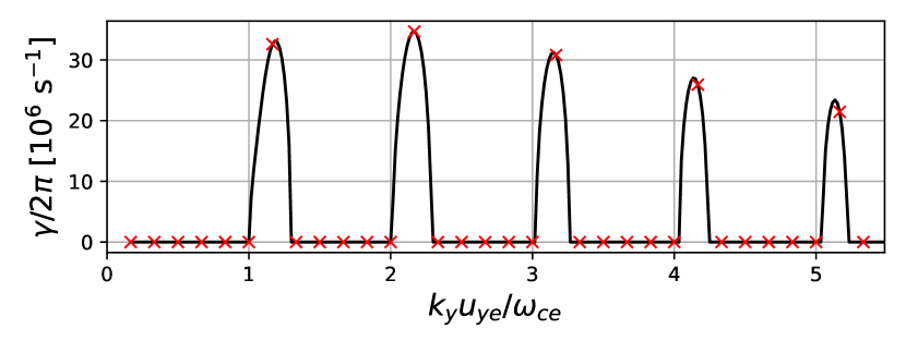
(b)

Figure 1: ECDI dispersion relation for a hydrogen plasma with $k_{\parallel}=0$, $k_{z}=0$ and the equilibrium conditions summarized in table 1. The black solid line is the solution for an infinite plasma. Red crosses stand for the discrete solutions in a finite plasma with $L_{y}=5.359$ mm. The blue solid line is the ion-acoustic frequency $\omega_{\textmd{IA}}$. The dispersion relation has been solved with the same numerical approach than reference [19].

If the plasma has a finite size $L_{y}$ along $y$, there is only a discrete wave spectrum with $k_{y}=n2\pi/L_{y}$ and $n$ the number of wavelengths fitting in the domain. Red crosses in Fig. 1 show that spectrum for $L_{y}=12\pi\ell_{e0}=5.359$ mm, when resonances correspond to $n$ a multiple of 6. That length has been chosen so that modes $n=1+6m$ capture approximately the peaks in $\gamma$ associated to each resonance $m$. For the chosen parameters, the fastest growing mode is $n=13$, close to the $m=2$ resonance, with $\gamma/2\pi=34.7\times 10^{6}$ s^-1, $k_{y}\ell_{e0}=2.167$ and $\omega_{r}=46.6$ MHz. In terms of growth rate, the mode $n=7$, in the band $m=1$, follows closely with $\gamma/2\pi=32.6\times 10^{6}$ s^-1, $k_{y}\ell_{e0}=1.167$ and $\omega_{r}=27.1$ MHz.

The effects of a nonzero (moderate) $k_{z}$ on the MIA modes are: introducing an ion-Doppler shift $k_{z}u_{zi0}$ in the frequencies, shifting the unstable bands in $k_{y}$, and changing mildly the growth rates (find a more exhaustive analysis in [18]).

To reduce the computational cost, simulations here correspond to a hydrogen plasma. The frequencies for hydrogen are, approximately, one order of magnitude higher than those expected in xenon. This is a reasonable result, since equation (4) shows that frequency and growth of the ECDI modes are proportional to $kc_{s0}$ and, thus, scale with $1/\sqrt{m_{i}}$. This trend is, indeed, retrieved in PIC simulations shown later in this paper. The use of hydrogen instead of xenon in PIC simulations of the ECDI is a computational advantage since it allows us to observe the same physical phenomena but in a shorter time. With the same time step (still limited by the electron dynamics), this means reducing the number of time steps by one order of magnitude.

III The classical ECDI: nonlinear evolution

III.1 The numerical PIC model

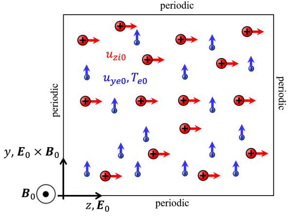
Figure 2: Diagram summarizing the simulation axes, boundary conditions and initial equilibrium state for simulations of the classical ECDI. A second type of simulations is considered that substitutes left and right boundary conditions to $\phi=0$ and injection/absorbing conditions for particles.

The nonlinear evolution and saturation of the classical ECDI is studied with a 2D axial azimuthal, 2D($z,\theta$), full PIC code developed in-house. The PIC formulation follows ions and electrons. The electrostatic potential is obtained from a Poisson solver. The numerical codes are implemented in Fortran and use OpenMP shared-memory parallel computing.

The PIC code applies a standard Boris method to move electron and ion macroparticles in the periodic domain, and it employs a particle-decomposition strategy for parallel calculations. Macroparticles have equal and constant weights (i.e., number of real particles per macroparticle). As already pointed out, collisions between particles are totally disregarded.

The Poisson solver is able to use different schemes depending on boundary conditions. When all boundaries are periodic (the case in the present section III), spectral methods are well suited to solve the Poisson equation in the Fourier complex space; here, the FFTW3 library [31] for Fourier and inverse transform operations is used, with a zero average potential. If Neumann or Dirichlet conditions are used in at least one boundary (the case in section IV), the Poisson solver uses a second order finite difference scheme for the Laplace operator and electric field, and the discrete linear system is solved with the PARDISO direct-solver routines in the Math Kernel Library of INTEL.

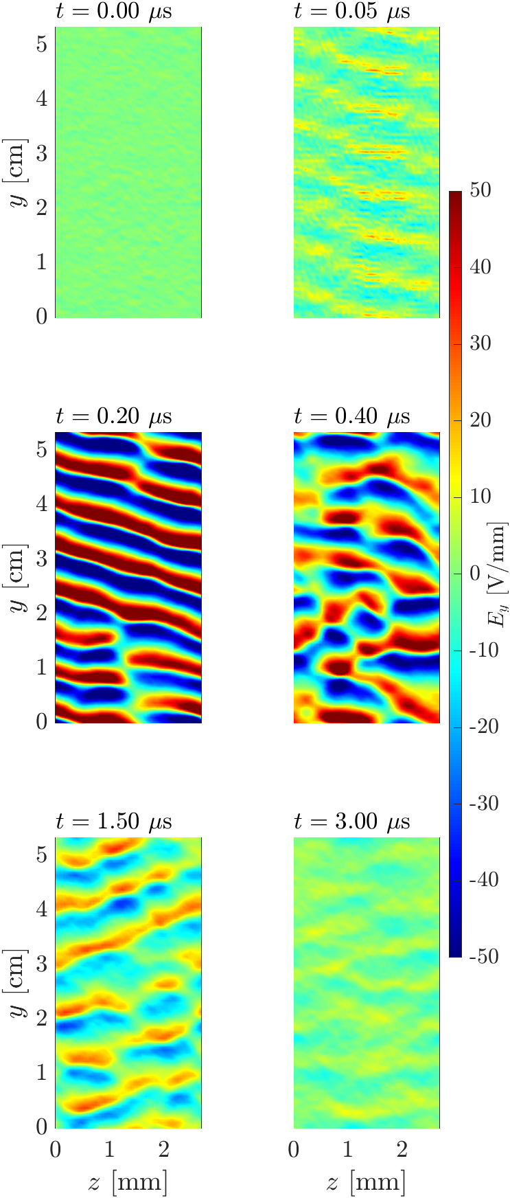
Figure 3: Reference case with fully periodic conditions: time-evolution of $E_{y}(y,z,t)$ in the $yz$-plane.

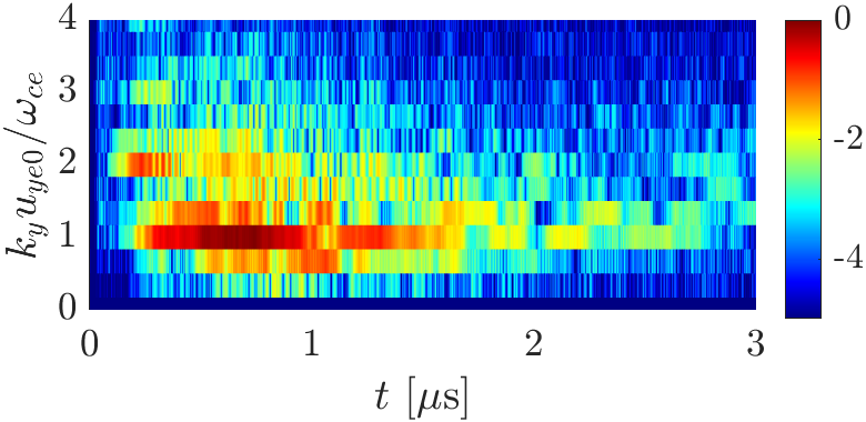
(a) $L_{y}=2.679\leavevmode\nobreak\ \textmd{mm}$

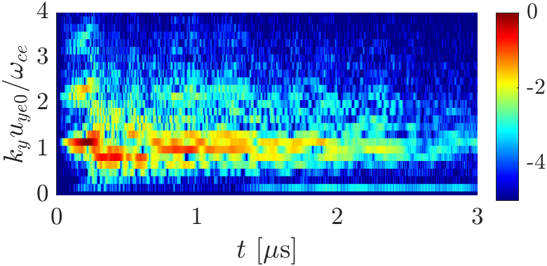
(b) $L_{y}=5.359\leavevmode\nobreak\ \textmd{mm}$

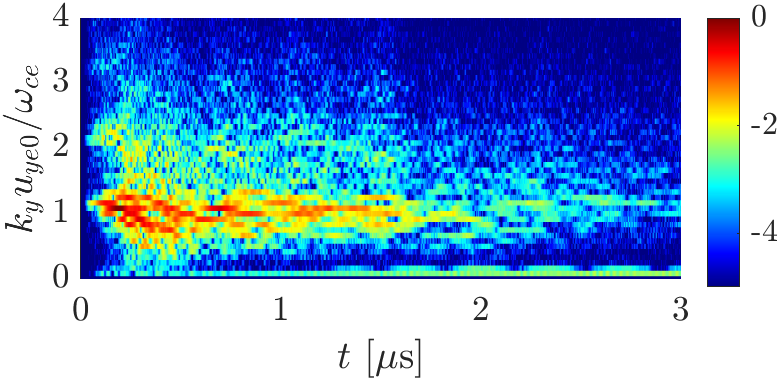
(c) $L_{y}=10.72\leavevmode\nobreak\ \textmd{mm}$

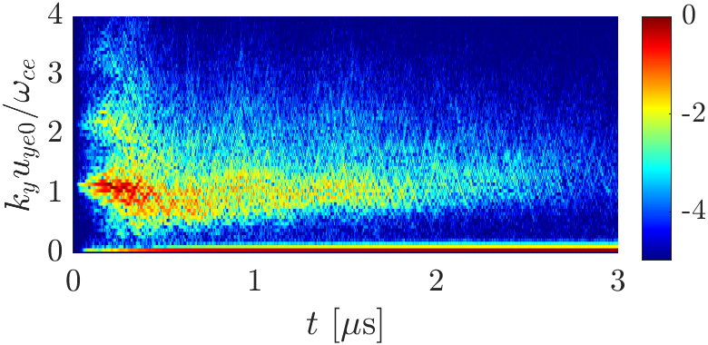
(d) $L_{y}=16.08\leavevmode\nobreak\ \textmd{mm}$

Figure 4: Reference case with fully periodic conditions: time-evolution of the logarithm of normalized coefficients from the fast Fourier transform of $E_{y}(t,y,z^{*})$ in coordinate $y$, at $z^{*}=5L_{z}/6$, for different $L_{y}$.

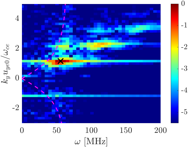
(a) $0\leavevmode\nobreak\ \mu\textmd{s}<t<0.20\leavevmode\nobreak\ \mu\textmd{s}$

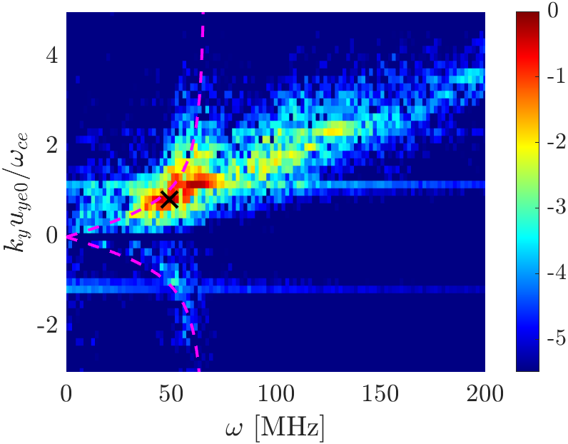
(b) $0.20\leavevmode\nobreak\ \mu\textmd{s}<t<0.75\leavevmode\nobreak\ \mu\textmd{s}$

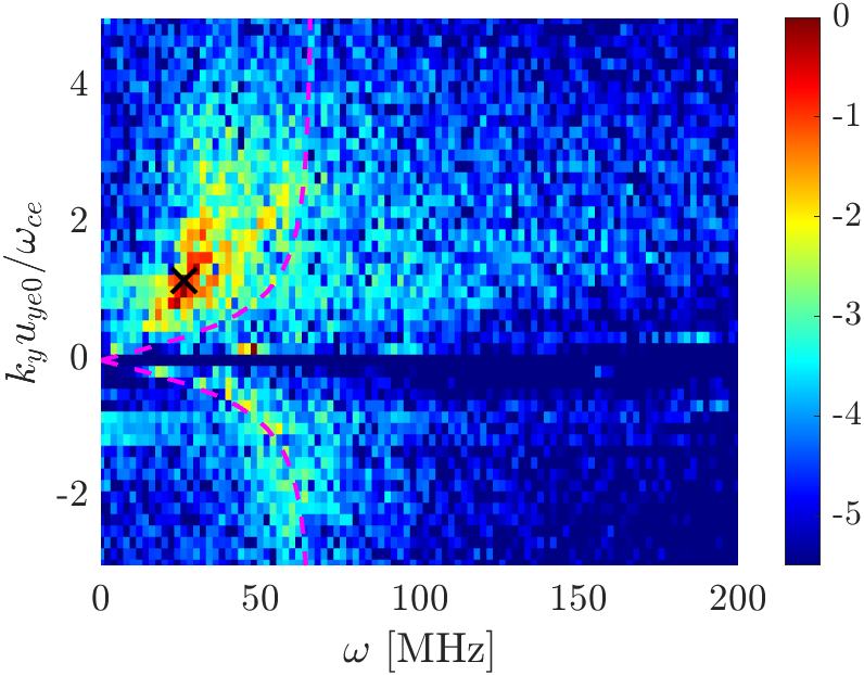
(c) $2.5\leavevmode\nobreak\ \mu\textmd{s}<t<3.0\leavevmode\nobreak\ \mu\textmd{s}$

Figure 5: Reference case with fully periodic conditions: logarithm of normalized coefficients from the 2D fast Fourier transform of $E_{y}(t,y,z^{*})$ in coordinates $y$ and $t$, at $z^{*}=5L_{z}/6$, and for 3 different time windows. The absolute maxima are marked with a black cross. Dashed magenta lines stand for ion-acoustic modes $\pm\omega_{\textmd{IA}}$ with $T_{e0}$ taken as the average value on the considered window: (a) 11.4 eV, (b) 40.1 eV and (c) 58.3 eV.

The electric and magentic fields felt by each species and their initial macroscopic properties comply with the hypotheses and equilibrium state of section II. That is to say, the initial electron population is randomly sampled from a Maxwellian VDF with density $n_{0}$, velocity $u_{ye0}\bm{1}_{y}$ and temperature $T_{e0}$. The initial ion population is generated with $n_{0}$ and $u_{zi0}\bm{1}_{z}$ without dispersion. The values of these properties and every other physical and numerical parameter are gathered in Table 1. The macroparticle weights are kept constant throughout the simulation and can be computed from initial conditions as $n_{0}\Delta y\Delta z/N_{\textmd{ppc}}$ Electron and ion particles are moved in a periodic domain with electric fields $\bm{E}_{e}=\bm{E}_{0}+\bm{E}_{1}$ and $\bm{E}_{i}=\bm{E}_{1}$, respetively, being $\bm{E}_{1}=-\nabla\phi$ the local fluctuation relative to $\bm{E}_{0}$ that comes as solution to the Poisson equation with periodic boundary conditions. Figure 2(a) sketches the simulation setup. At the initial equilibrium state, the axial current of electrons, $j_{ze0}$ is zero. Any subsequent electron axial current is due to the cross-field transport generated by plasma oscillations.

Regarding the macroscopic and kinetic results to be shown, they include a moving-average during runtime on a window corresponding to $N_{\textmd{print}}$ time steps. For an arbitrary variable $\varphi$, this is defined as

$$\tilde{\varphi}_{k}=\frac{\tilde{\varphi}_{k-1}(N_{\textmd{print}}-1)+\varphi_{k}}{N_{\textmd{print}}},$$ (8)

being $k$ the time step index, $\varphi_{k}$ the instantaneous value of and $\tilde{\varphi}_{k}$ its time-average value.

III.2 Onset, saturation, and vanishing of the ECDI

The time evolution in the $yz$-plane of $E_{y}(t,y,z)$ is represented in figure 3. The initial equilibrium state is unstable and the ECDI start to grow from any perturbation. The time-dependent solution is almost 1D in the azimuthal direction, although an axial component is present in early times, mainly. The oscillation amplitude gets a maximum around 0.2 $\mu$s and decreases in later times until eventually a new equilibrium state, different from the initial one, is reached. For $t<0.2\leavevmode\nobreak\ \mu$s, wave modes are weakly mixed and the dominant monochromatic waves are easier to observe. The top panels of figure 3 indicate that the dominant mode is $n=7$, which is the closest one to the resonance $m=1$. For $t>0.2\leavevmode\nobreak\ \mu$s, there is more mixing of modes; the bottom panels of figure 3 show transitions to $n=5$ and 6 as dominant modes.

The linear theory showed that mode $m=2$ has a (slightly) higher growth rate than mode $m=1$. In fact the Fourier analysis of $E_{y}(t,y,z)$ in $y$ [depicted in figure 4(b) for our simulation with $L_{y}=5.359$mm] shows some contribution of mode $m=2$ to the early time spectrum. However, the fast growth of several modes makes nonlinear effects important soon in the simulation, which, together with the noise intrinsic to the PIC formulation, makes tough the exact comparison of early PIC results with the linear results from Vlasov equation [29, 32]. In addition, the long-term dominant modes in the nonlinear stage may not coincide with the most unstable modes in the linear dispersion relation [21]. The use of quiet start techniques by other authors [32, 22] to minimize the noise of the initial population has not been seen to be completely satisfactory.

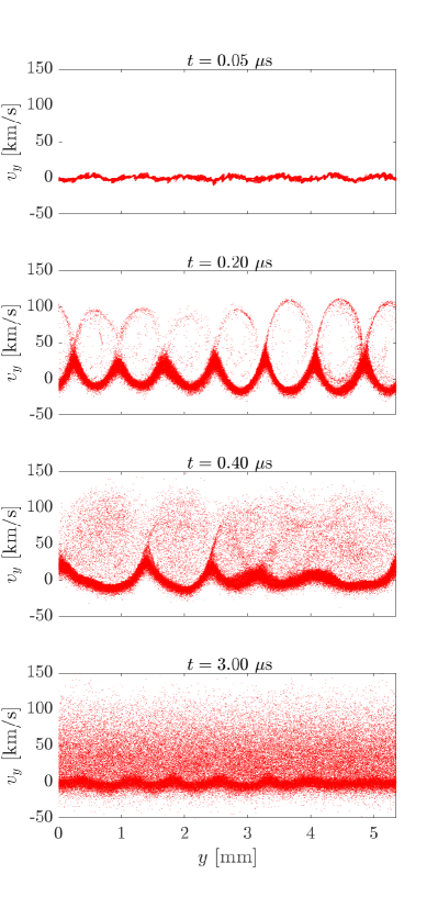
Figure 6: Reference case with fully periodic conditions: time evolution, in the phase space $(y,v_{y})$, of ions contained in an axial slab of width $0.1L_{z}$. The formation and blurring of the vortex-like structure characteristic of ion-wave trapping is observed.

The determination of the dominant frequency is more difficult since it depends on time itself. In Figure 5, results of the 2D fast Fourier transform in $y$ and $t$ are shown for three different time windows, together with the ion-acoustic curves $\pm\omega_{\textmd{IA}}$ for the average $T_{e}$ within the corresponding time interval. Each window represents different stages in the evolution of the ECDI:

• $0<t<0.20\leavevmode\nobreak\ \mu\textmd{s}$. The peaks seem to concentrate in bands near $k_{y}\ell_{e0}=m$, similarly to the theoretical dispersion relation in figure 1. The maximum Fourier coefficient is located at $k_{y}\ell_{e0}=1.166$ and $\omega_{r}=55.6$ MHz, with phase speed $\omega_{r}/k_{y}=42.6$ km/s. This is mode number $n=7$, near the resonance $m=1$. There are secondary bands close to $m=2$ and $m=3$. The results in this early stage are qualitatively aligned with figure 1, but the dominant frequency $\omega_{r}$ is larger than predicted by the linear theory.

• $0.2\leavevmode\nobreak\ \mu\textmd{s}<t<0.75\leavevmode\nobreak\ \mu\textmd{s}$. The bands of the upper spectrum near the resonances have been blurred and there is an approximately linear relation between $k_{y}$ and $\omega_{r}$, resembling a linear ion-acoustic relation. However, some parts of the upper spectrum seem to follow the non-neutral acoustic frequency $\omega_{\textmd{IA}}$. This is aligned with previous PIC simulations[23, 28] and experiments[4]. The peak in the spectrum is at $k_{y}\ell_{e0}=0.8334$; with $n=5$, $\omega_{r}=49.1$ MHz and $\omega_{r}/k_{y}=52.6$ km/s and matches the ion-acoustic curve. Let us note that the lower part of the spectrum (propagation in the $-\bm{E}_{0}\times\bm{B}_{0}$ direction), shows some remnants of the counter-propagating ion-acoustic wave with frequency $-\omega_{\textmd{IA}}$.

• $2.5\leavevmode\nobreak\ \mu\textmd{s}<t<3\leavevmode\nobreak\ \mu\textmd{s}$. Even if a peak is identifiable at $k_{y}\ell_{e0}=1.166$ ($n=7$), the mixing of different temporal and azimuthal scales result in a messy spectrum without a clear dominant mode. The ion-acoustic behavior is only seen in the lower part of the spectrum.

At $t\sim 3\leavevmode\nobreak\ \mu\textmd{s}$, the plasma seems to tend to a new equilibrium with distorted ion and electron VDFs. Figure 6 plots the evolution of ion particles, contained within an axial slab of width $0.1L_{z}$, in phase space $(y,v_{y})$. During the growth and saturation of the ECDI (this is $t<0.2\leavevmode\nobreak\ \mu$s), vortexes are formed in phase space showing the characteristic behavior of ion trapping in the electrostatic wave. The vortexes are shifted towards positive velocities, matching the $\bm{E}_{0}\times\bm{B}_{0}$ and dominant mode propagation directions. Later times reveal the distortion of those vortex structures until they are fully blurred into a strongly one-sided distribution with a long tail into positive velocities. This process coincides with the quenching of $E_{y}$ oscillations. Electrons one-dimensional VDFs at the end of the simulation are shown in figure 7 to be fairly isotropic and flatter close to the average velocity compared to a Maxwellian, which coincides with [25, 18].

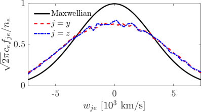
Figure 7: Reference case with fully periodic conditions: normalized electron distribution functions $f_{je}$ in the azimuthal ($j=y$, red dashed) and axial ($j=z$, blue dash-dotted) directions, being the abscissa coordinate $w_{je}$ the random velocity of electrons . The Maxwellian curve (black solid) is included for comparison, using local final values of $n_{e}=10^{17}$ and $T_{e}=58.8$ eV from the PIC simulation.

III.3 Evolution of the plasma energy

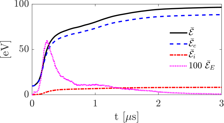
(a) Energy

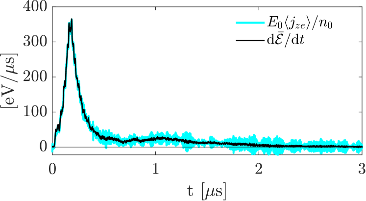
(b) Energy derivative

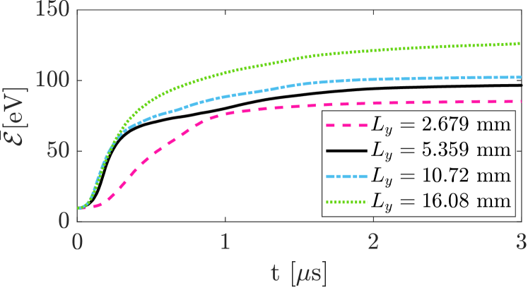
(c) Effect of $L_{y}$ on $\bar{\mathcal{E}}$

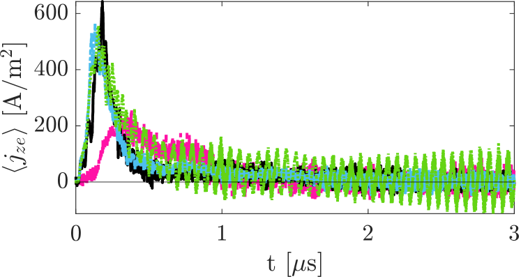
(d) Effect of $L_{y}$ on $\left\langle j_{ze}\right\rangle$

Figure 8: Fully-periodic case. Time evolution of (a) the energy time-derivative and (b) the electrostatic, species and total energies per particle (i.e., $\bar{\mathcal{E}}=\mathcal{E}/\left\langle n\right\rangle V$. Panels (c) and (d) plot energy per particle and volume-averaged electron axial current for different $L_{y}$.

Let us get a further insight on the ECDI by analyzing the plasma energy stored in the plasma. The total energy in the plasma domain has contributions from the electrostatic field, electrons and ions, according to

$$\mathcal{E}=\mathcal{E}_{E}+\mathcal{E}_{e}+\mathcal{E}_{i},$$ (9)

with

$$\mathcal{E}_{E}=\frac{\varepsilon_{0}}{2}\int_{\mathcal{V}}E_{1}^{2}\leavevmode\nobreak\ \text{d}\mathcal{V}.$$ (10)

the energy of the electromagnetic oscillations,

$$\mathcal{E}_{s}=\int_{\mathcal{V}}\left[\frac{1}{2}m_{s}n_{s}u_{s}^{2}+\frac{3}{2}p_{s}\right]\text{d}\mathcal{V},\quad s=e,i$$ (11)

the total energy of electrons and ions; and $\mathcal{V}$ is the volume of the domain. For convenience, the equilibrium field $\bm{E}_{0}$ has been omitted from the definition of $\mathcal{E}_{E}$, since it would only introduce a constant offset in the energy. The energy of each species is approximated in the PIC formulation as

$$\mathcal{E}_{s}=\sum_{p}\frac{1}{2}m_{s}v_{p}^{2}W_{p},$$ (12)

where the sum is on every particle in the domain with $v_{p}$ and $W_{p}$ the particle speed and weight, respectively.

In a consistent situation, the work done by the electric field should act as a mechanism that converts species energy on electric-field energy, and the other way around. However, the assumptions behind the linear theory of the ECDI forced us to let ions and electrons feel different electric fields. Because of this non-conventional feature, it can be proved that the total energy changes according to

$$\frac{\partial\mathcal{E}}{\partial t}=\int_{\mathcal{V}}(\bm{j}_{e}\cdot\bm{E}_{0})\leavevmode\nobreak\ \text{d}\mathcal{V}=E_{0}\int_{\mathcal{V}}j_{ze}\leavevmode\nobreak\ \text{d}\mathcal{V}=E_{0}\langle j_{ze}\rangle\mathcal{V},$$ (13)

with $\bm{j}_{e}$ the electron current density and $\langle j_{ze}\rangle$ the volume-averaged $j_{ze}$. Therefore, this kind of simulation will not show a proper conservation of energy and the equilibrium electric field will pump energy into the isolated system. However, this source of energy requires also an axial electron current $j_{ze}$ to be developed. This means that the energy is conserved initially until the instability is triggered, and any other stationary energy state should satisfy a null $\langle j_{ze}\rangle$, i.e., no turbulent electron transport.

Figure 8(a) shows the evolution of electrostatic, species, and total energies in the domain per real particle. Here, average energies per particle $\bar{\mathcal{E}}=\mathcal{E}/\left\langle n\right\rangle\mathcal{V}$ are used, being $\left\langle n\right\rangle$ the volume-averaged density and $\left\langle n\right\rangle\mathcal{V}$ the real number particles in the domain. Initially $\bar{\mathcal{E}}_{E}=0$, $\bar{\mathcal{E}}_{i}=m_{i}u_{zi0}^{2}/2=0.0324$ eV and $\bar{\mathcal{E}}_{e}=3T_{e0}/2+m_{e}u_{ye0}^{2}/2=9.71$ eV. Eventually, the total energy saturates and becomes stationary. There is significant heating of electrons and, to a lesser extent, of ions; which is coherent with other works [29, 25, 22, 26]. The electrostatic energy is much lower than those of electrons and ions, and approaches zero for late simulation times, when oscillations are very weak.

The balance (13) is evaluated in figure 8(b). The rate $\textmd{d}\bar{\mathcal{E}}/\textmd{d}t$ is approximated numerically and compared with the source term $E_{0}\langle j_{ze}\rangle/n_{0}$. The two curves show an excellent match apart from the noise inherent to the PIC approach, specially problematic in the calculation of $j_{ze}$. The PIC simulation is able to approximately replicate the theoretical energy balance (13), which is a good sign of the validity of such simulations. The change in energy shows a peak and then decreases tending to zero for late simulation times, meaning that a new stationary equilibrium state of the plasma is reached. As already said, the energy source is related with the development of a net axial current, so the new equilibrium holds an average $j_{ze}$ equal to zero. However, at mid simulation times, saturated ECDI modes are effective in inducing an axial transport of electrons.

III.4 Effect of the domain’s azimuthal length

As pointed out in section II, the azimuthal domain length $L_{y}$ is an important parameter that determines the unstable ECDI modes that can be excited in a finite domain. On the contrary, the effect of $L_{z}$ has been seen to be small, although the chosen axial length is large enough to allow the formation of waves with axial component fitting $L_{z}$. Increasing $L_{y}$ allows larger scales to develop and increases the spectral resolution in the $k_{y}$-space, better capturing the continuous dispersion relation for an infinite plasma. In figure 4, the time evolution of azimuthal Fourier coefficients for $E_{y1}$ are represented for several $L_{y}$ multiples of 2.679 mm, the reference case corresponding to plot 4(b). The main trends identified in the shortest case are also recovered in larger domains: modes close to resonant bands $m=1$ and $m=2$ are excited in early times, modes close to $m=1$ dominate at mid times, and oscillations quench after the spectrum peaks are passed. These trends become clearer as longer domains are used. Some differences worth mentioning among cases are: (i) a mode with azimuthal wavelength equal to $L_{y}$ (i.e. $n=1$) is present only at long $L_{y}$ and (ii) the enhanced spectral resolution of longer $L_{y}$ allows to better capture shorter resonant bands, such as the modes close to $m=2$. Similar conclusions on these two points are reached in reference [29].

Figure 8(c) shows that the energy per real particle increases with parameter $L_{y}$, probably due to the greater number of unstable excited modes [29]. With the exception of the shortest case $L_{y}=2.679$ mm, which shows a slower energy increase and lower $\langle j_{ze}\rangle$ [most probably due to a poor spectral resolution, unable to properly capture the peaks of the growth rate of Fig 1] the rates of energy increase during the growth period are similar for $L_{y}\geq 5.359$ mm. This suggests that the maximum $\langle j_{ze}\rangle$ and the time to reach it are numerically robust and thus physical. Therefore, results with $L_{y}=5.359$ mm are representative of simulations with longer $L_{y}$ multiples of 5.359 mm. This behavior disagrees with reference [29], where changes in $L_{y}$ can drastically change the transients of $\langle j_{ze}\rangle$ and, thus, the energy growth rates.

Since the long term behavior of $\langle j_{ze}\rangle$ tends to zero in every case, we can conclude that the long-wavelength mode with $n=1$ that develops with increasing $L_{y}$ is not effectively producing an axial electron transport. This is consistent with the late evolution of $n_{e}$ and $E_{y}$ (not included), which shows completely out of phase oscillations.

III.5 Effect of the ion mass

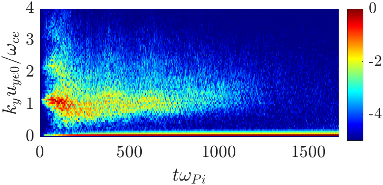
(a) $m_{i}=1\textmd{u}$

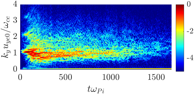
(b) $m_{i}=4\textmd{u}$

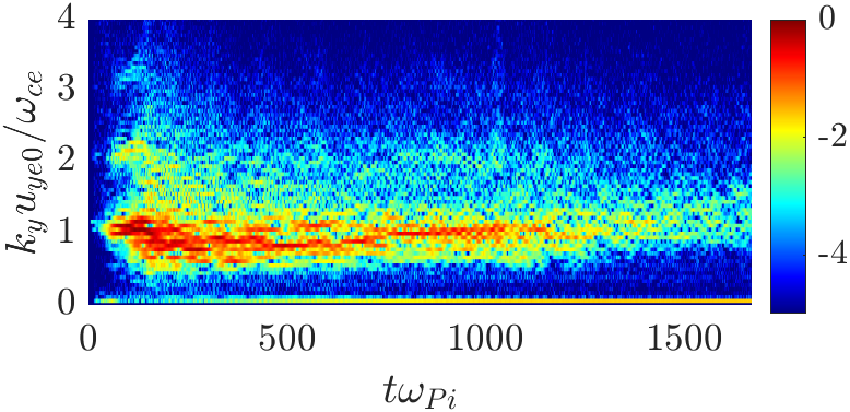
(c) $m_{i}=9\textmd{u}$

Figure 9: Fully-periodic case, Time-evolution of the logarithm of normalized azimuthal Fourier coefficients for different values of $m_{i}$.

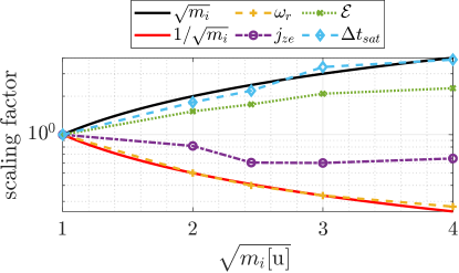
Figure 10: Scaling factor, with the ion mass $m_{i}$, of several variables: dominant $\omega_{r}$ in the interval $t\omega_{Pi}<83.15$, peak averaged $j_{ze}$, final $\mathcal{E}$ and $\Delta t_{\textmd{sat}}$. The curves $\sqrt{m_{i}}$ and $1/\sqrt{m_{i}}$ are also included for comparison.

In this subsection, the simulation is repeated for increasing values of the ion mass. While hydrogen mass, $m_{H}$ has been used in order to speed up the dynamics and minimize the computational cost, the practical cases of interest deal with heavier ions, e.g., xenon or krypton. In addition, an increased azimuthal length $L_{y}=16.08$ mm is used to have a proper spectral resolution and a fair comparison, since an increased $m_{i}$ narrows the unstable bands in the dispersion relation near the resonances what needs an increased spectral resolution.

In the early evolution of the ECDI, the dispersion relation (4) shows that the frequency should scale inversely proportional to $\sqrt{m_{i}}$. However, this does not have to be the case of the nonlinear dynamics or other magnitudes. The scaling factors for several quantities, defined as the ratio with respect to the value in the reference case $m_{i}=1$ u are computed in figure 10: dominant $\omega_{r}$ in the interval $t\omega_{Pi}<83.15$, peak of $\left\langle j_{ze}\right\rangle$, final $\mathcal{E}$ and $\Delta t_{\textmd{sat}}$. The observed trends are coherent with results reported in reference [33]. If the dominant frequency is measured in early simulation times, the observed scaling perfectly matches the linear theoretical result. The saturation time $\Delta t_{\textmd{sat}}$, defined as the time of maximum average $\left\langle j_{ze}\right\rangle$, seems to scale proportional to $\sqrt{m_{i}}$. The 1D azimuthal Fourier spectra are compared in figure 9, where the time axis is normalized with the inverse of the ion plasma frequency $\omega_{Pi}$. While the saturation of the early oscillations produced by the ECDI happens at similar $t\omega_{Pi}$ (as shown by the scaling of $\Delta t_{\textmd{sat}}$), the quenching of short wavelength $m=1$ and $\left\langle j_{ze}\right\rangle$ seems to be slightly slower with increasing $m_{i}$.

The level of turbulent current, measured by the peak $\left\langle j_{ze}\right\rangle$, initially decreases with $m_{i}$, which could be explained by the weaker oscillations observed in $n_{e}$ (not included here), but seems to saturate. The current $\left\langle j_{ze}\right\rangle$ decreases, however, slower than $1/\sqrt{m_{i}}$ which leads to a final $\mathcal{E}$ increasing with $m_{i}$, in accordance with equation (13). Extrapolating these results, with xenon we can expect somehow smaller level of transport but dilated in time, what would cause a significant heating such as that observed in similar studies in the literature [22, 21, 29].

III.6 Saturation behavior in previous literature

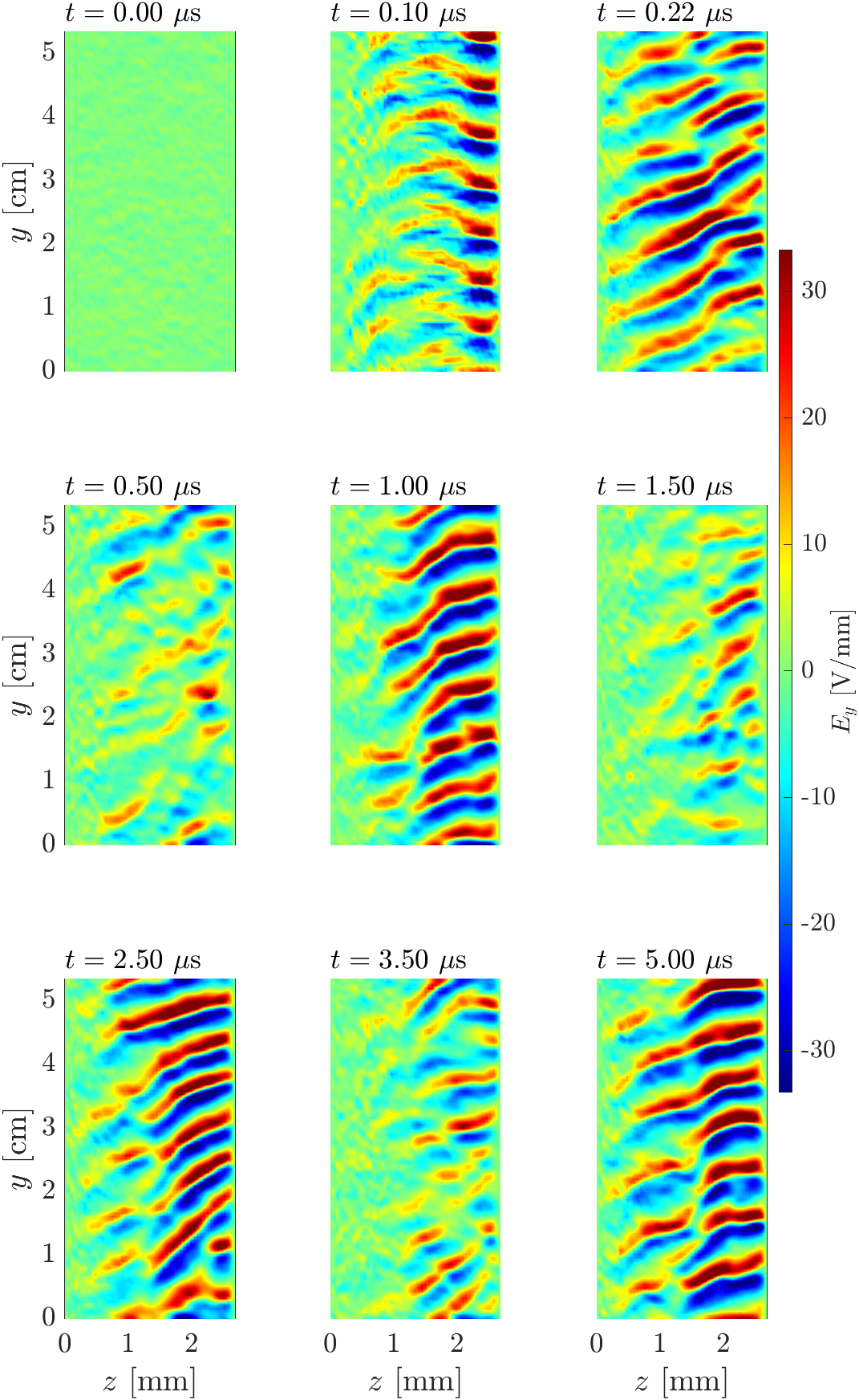
Figure 11: Finite plasma with axial injection. Time-evolution of $E_{y}$ in the $yz$-plane.

The results we have shown in this section pursue the simulation of scenarios as close as possible to the classical ECDI. While we observe the growth and saturation of oscillations due to an instability, modes that induce an axial electron transport seem to vanish at long times. The late simulation behavior differ from other 1D [25, 22, 26, 29] and 2D [23, 28, 17, 24] simulations on similar configurations, which report sustained oscillations not vanishing with time. Even if our model is 2D, we disregard many of the effects included in other 2D works (e.g., inhomogeneous magnetic field, anode-cathode circuit or collisions), which are closer to Hall-discharge-like configurations. A fairer comparison is that with the existing 1D azimuthal models [25, 22, 26, 29], whose sustained oscillation for late simulation times either saturate[22, 26] or forever grow [25, 29], depending on the axial treatment of particles.

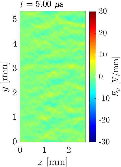
(a) $u_{zi0}=1\leavevmode\nobreak\ \textmd{km/s}$

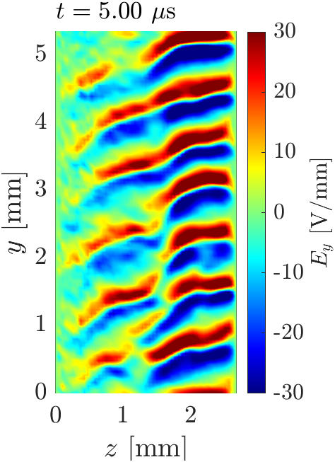
(b) $u_{zi0}=10\leavevmode\nobreak\ \textmd{km/s}$

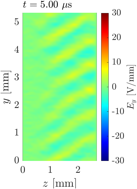
(c) $u_{zi0}=100\leavevmode\nobreak\ \textmd{km/s}$

Figure 12: Finite plasma with axial injection. Late behavior (at $t=5\mu$s) of $E_{y}$ in the $yz$-plane, for different $u_{zi0}$.

As seen in section III.2, the stages observed in the evolution of oscillations are greatly related to the interaction of ions with the electrostatic wave and the distribution of ion particles in phase space. Our approach, similarly to references [25, 29], disregard $\bm{E}_{0}$ on the ion motion to prevent the consequent axial inhomogeneity and be able to apply periodic conditions, not only azimuthally, but also axially. Because there is no change in velocity for particles going through boundaries, the change in the VDF of ions and electrons from the initial one is solely a result of the ECDI. On the other hand, references [22, 26] account for a virtual axial dimension, so that particles that leave the domain through axial boundaries after interacting with the electrostatic wave are re-injected with a refreshed velocity sampled from a prescribed VDF. This is, the refreshing axial conditions (and the refreshing rate determined but the axial length) modify the VDF of particles and can have a significant impact on the particle-wave interaction and overall simulation behavior. This point is extensively analyzed in the next section.

When no virtual axial dimension or refreshing are considered, previous literature [29, 25, 22] observe an unlimited growth of the oscillations and heating. The reasons that explain why they do not see the quenching of short-wavelength waves are still to be investigated, but let us speculate about a couple of possibilities. An explanation could be that the evolution towards a new equilibrium is not inherent to all simulations of this type and depends on the selection of parameters (although this is the behavior we have seen in all of our simulations). Another possibility, in line with the results in section III.5, could be that more simulation time is needed with xenon than considered in [29, 25, 22] to observe our late simulation stage.

IV THE ECDI IN AN AXIALLY-INJECTED FINITE-PLASMA

In the previous section, we pointed out the possible interaction of particle injection with the ECDI. Fully periodic boundary conditions preserve the VDF of the particles resultant of interacting with the instability. When there is particle removal and injection through boundaries, particles that have already interacted with the wave are removed from the simulation and new particles are injected having a different VDF that could possibly modify the behavior of the instability.

Following this reasoning, a new simulation setup is presented here that replaces axial periodic conditions by injection ones, while periodic conditions are kept in the azimuthal direction. Any particle leaving the domain though axial boundaries is removed from the simulation. A constant flux of ions $n_{0}u_{zi0}$ is injected through the left boundary, with zero temperature and velocity $u_{zi0}\bm{1}_{z}$. Constant fluxes of electrons $\pm n_{0}c_{e0}/\sqrt{2\pi}$, corresponding to a half-Maxwellian, are injected through left and right boundaries, whose velocities are sampled from a Maxwellian VDF with temperature $T_{e0}$ and velocity $u_{ye0}\bm{1}_{y}$. The injection fluxes are chosen such that they match the amount of ions and electrons leaving the domain in equilibrium conditions, making this equilibrium equivalent to the fully periodic domain. In contrast with the particle refreshing approach used in [22, 26], once the instability arises, the injected fluxes do not need to coincide with fluxes leaving the domain and the number of particles and electric charge are not conserved anymore. For that reason, axial conditions on potential are also changed from periodic to fixed potential $\phi=0$ and the finite-difference PARDISO version of the Poisson solver is used.

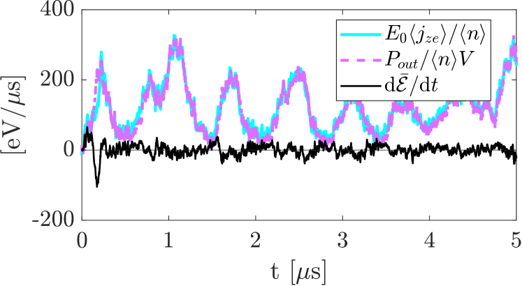
(a) Energy balance

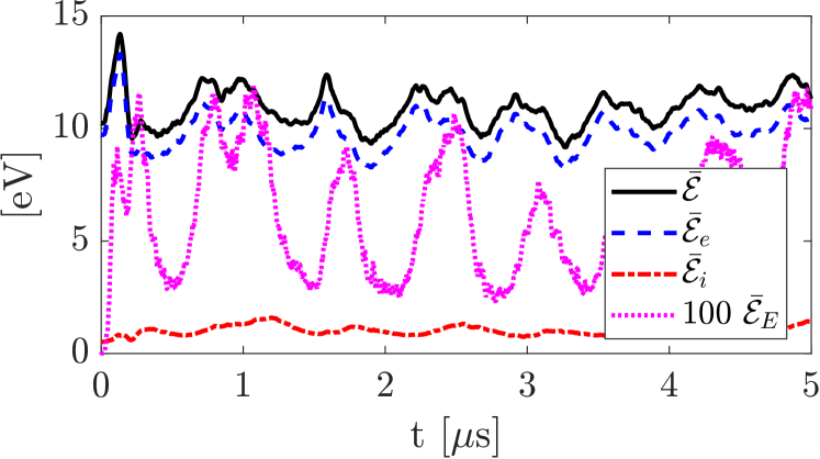
(b) Total and species energies

Figure 13: Finite plasma with axial injection. Time evolution of (a) energy balance and (b) electrostatic (c), species and total energies; for an axial-injection simulation with $u_{zi0}=10$ km/s. Values are given per real particle.

IV.1 Dependence on the ion residence time

In section III, we showed the usual stages that we observe in the evolution of the ECDI, being the final one the quenching of short-wavelength oscillations. These stages are related with the ion velocity distribution and the formation and blurring of vortex-like structures in phase space. In this sense, adding axial boundaries that inject and absorb particles can have a major impact on the late simulation behavior since old particles that have interacted with the wave are removed and new, non-trapped particles are injected with the original distribution.

In this scenario with axial injection, more similar to a Hall discharge, the ion residence time

$$\Delta t_{i0}=L_{z}/u_{zi0}$$ (14)

(infinite in a fully periodic domain independently of $L_{z}$) is the key parameter in maintaining a saturated ECDI, with sustained short-wavelength oscillations and a nonzero axial electron transport. Three regimes will be distinguished depending on $\Delta t_{i0}$ being much smaller, of the same order, or much higher than the saturation time $\Delta t_{\textmd{sat}}$ of the full-periodic configuration for the same equilibrium plasma, where $\langle j_{ze}\rangle$ peaks.

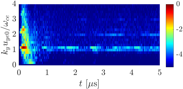
(a) $u_{zi0}=1$ km/s

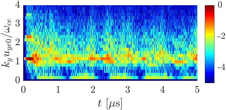
(b) $u_{zi0}=5$ km/s

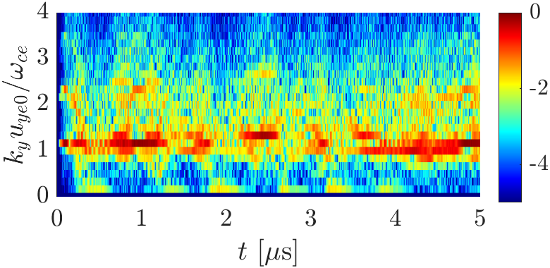
(c) $u_{zi0}=10$ km/s

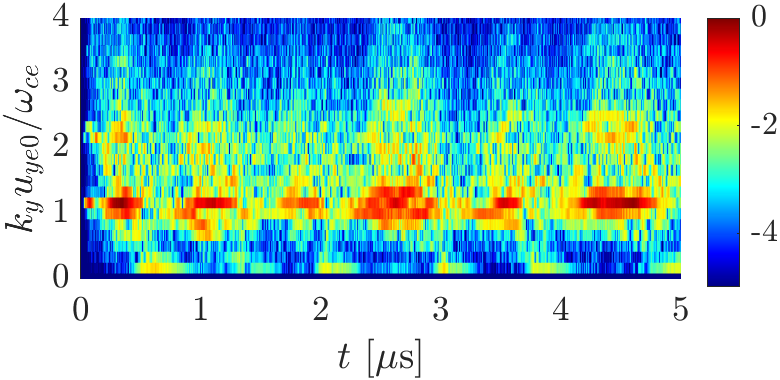
(d) $u_{zi0}=15$ km/s

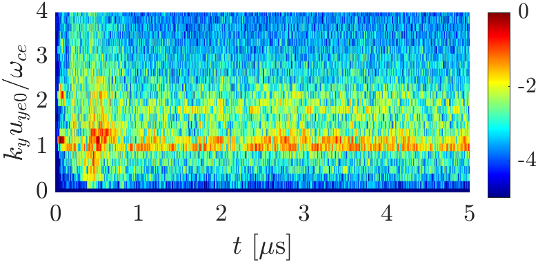
(e) $u_{zi0}=25$ km/s

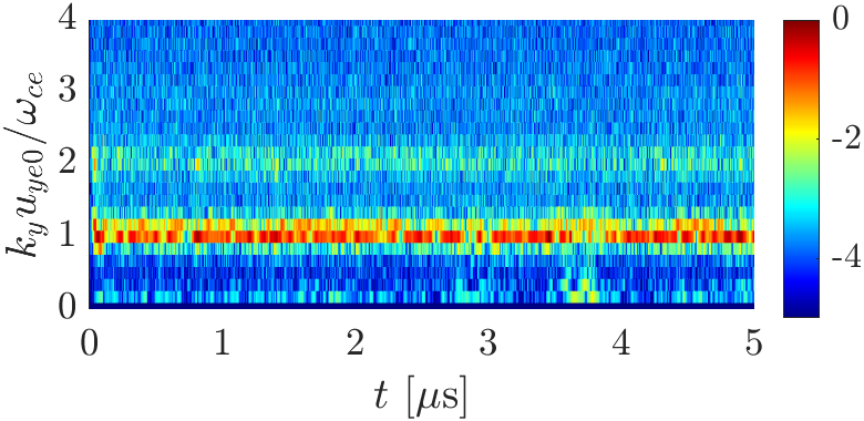
(f) $u_{zi0}=100$ km/s

Figure 14: Finite plasma with axial injection. Time-evolution of the logarithm of normalized azimuthal Fourier coefficients for different values of $u_{zi0}$.

We consider again a hydrogen plasma and the reference case of Table 1. The saturation time was $\Delta t_{\textmd{sat}}\sim 0.16$-0.18 $\mu$s. We run cases with $u_{zi0}=1$, 5, 10, 15, 20, 25 and 100 km/s, yielding, for $L_{z}=2.679$ mm, residence times $\Delta t_{i0}=2.68$, 0.536, 0.268, 0.179, 0.134, 0.107 and 0.0268 $\mu$s, covering the three expected regimes.

The evolution of azimuthal Fourier coefficients in figure 14 and the average current $j_{ze}$ in figure 15 give an idea of the time evolution, where the transition from one limit regime to the other can be appreciated. The final $E_{y}$ in the axial-azimuthal plane after $5\leavevmode\nobreak\ \mu$s for cases $u_{zi0}=1$, 10 and 100 km/s are shown in figure 12.

The case having $u_{zi0}=1$ km/s corresponds to regime $\Delta t_{i0}\gg\Delta t_{\textmd{sat}}$ and the final $E_{y}$ resembles the periodic case. Looking at figure 14(a), we see that the time evolution of Fourier coefficients is only similar at very early times when the onset of the ECDI on the initial population; after which oscillations are mild. From the energy point of view, the different axial boundary conditions here limit the electron heating and total energy in the domain, which is probably limiting the energy and contributing to the quenching of oscillations after the first ECDI onset. The evolution of $\langle j_{ze}\rangle$ is similar to the periodic case, where the current induced by the onset of the ECDI at early simulation times fades away at large enough times.

On the opposite limit we have the case $u_{zi0}=100$ km/s with $\Delta t_{i0}\ll\Delta t_{\textmd{sat}}$, where the final $E_{y}$ shows a sustained but very weak short-wavelength oscillation. The azimuthal spectrum shows that dominant modes concentrate around resonancea $m=1$ and, to a lesser extend, $m=2$. In this regime ECDI modes cannot develop completely since most of the ions leave the domain before full trapping occurs, so that we get an early stage of the ECDI observed with periodic conditions. According to figure 15, these mild oscillatory modes induce a weak $j_{ze}$ in the electrons, which is very small compared with values produced by a fully developed ECDI.

In the intermediate regime $\Delta t_{i0}\sim\Delta t_{\textmd{sat}}$ we consider cases with $u_{zi0}$ between 5 and 25 km/s (always for hydrogen). The plasma behavior resembles the saturated behavior of periodic simulation, because the removal and injection of particles happen at the proper rate that keeps feeding ECDI modes and allows them to fully develop, preventing the quenching of the oscillations observed in the regime $\Delta t_{i0}\gg\Delta t_{\textmd{sat}}$. From these cases, those with $u_{zi0}=5$ and 25 km/s are halfway between regimes and show features of both limit and intermediate regimes. In every case, the electric field shows sustained oscillations with a clear dominant mode close to the resonance $m=1$, that effectively induces a significant $j_{ze}$ in the long term. The magnitude of the induced transport depends on the case, being more significant, and comparable to the peak values of the periodic case, for the cases with $u_{zi0}=10$ and 15 km/s. In these two cases the dominance of modes close to $m=1$ does not happen at every time and there is some kind of intermittent or pulsed behavior of long and short wavelength modes, which results in an oscillatory evolution of the average $j_{ze}$. This intermittency is also observed in the time evolution of figure 11 for the case $u_{zi0}=10$ km/s. For greater and smaller values of ion velocity, $j_{ze}$ gets diminished, which is expected after our observations of null $j_{ze}$ in upper and lower limit regimes.

From the point of view of ion particles in phase space, the final pictures for cases $u_{zi0}=1$, 10 and 25 km/s are shown in an axial slab $0.7<z/L_{z}<0.75$. Here, it is confirmed that only when $\Delta t_{i0}\sim\Delta t_{\textmd{sat}}$ the vortex-like structure characteristic of ion-wave trapping is preserved and long-term axial transport exists. The existence of different regimes depending on the ion residence time could also explain why, with a virtual axial length, some groups observe a transition to an ion-acoustic mode [20] while others do not [26, 34].

The sensitivity of these results to $L_{y}$ has been tested to ensure that the same conclusions apply to larger domains. The evolution of electron currents are plotted in figure 17 varying $L_{y}$ while fixing $u_{zi0}=10$ km/s. As with fully periodic simulations, the shortest case gives the most different transient but in all cases a large $j_{ze}$ develops and they all show the characteristics of the intermediate regime $\Delta t_{i0}\sim\Delta t_{\textmd{sat}}$. In light of the fully periodic results, where larger $L_{y}$ seemed to favor the formation of long domain-size modes, it is surprising that, here, increasing $L_{y}$ mitigates the intermittency of short and long scales and yields less oscillatory currents. A possible explanation could be that the saturation time is slightly affected by $L_{y}$.

Previous results can be extrapolated to xenon in a Hall discharge using the scaling laws suggested in section III.5 and a typical $\Delta t_{i0}$. Using an average ion velocity $u_{zi0}=17$ km/s and anode-to-cathode length $L_{z}=3.35$ cm (e.g., from results in [35]), $\Delta t_{i0}$ is estimated to be 1.95 $\mu$s. The value of $\Delta t_{\textmd{sat}}$ for xenon mass is estimated to be 1.83 to 2.06 $\mu s$. This similarity suggests that the intermediate regime of the ECDI in a finite plasma could develop in a conventional Hall discharge and supports the idea of the ECDI possibly being an important actor in the anomalous electron transport.

IV.2 Energy balance

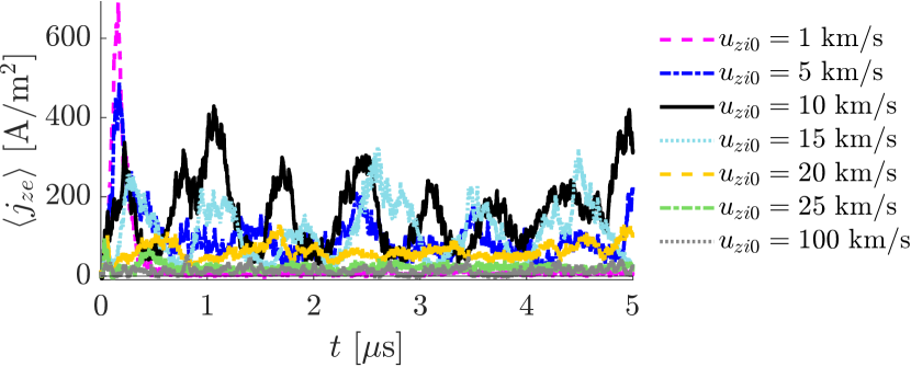
(a) Axial electron current

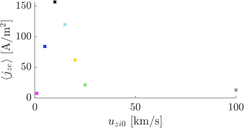
(b) Time-averaged $\left\langle j_{ze}\right\rangle$

Figure 15: Finite plasma with axial injection. (a) Time evolution of the volume-averaged electron axial current $\left\langle j_{ze}\right\rangle$ for several $u_{zi0}$ and (b) its time average for $t\geq 2$ $\mu$s.

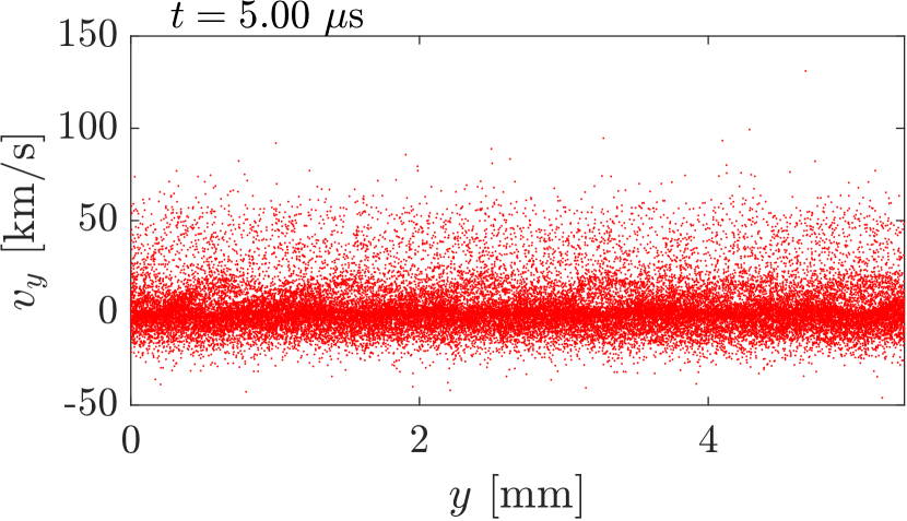
(a) $u_{zi0}=1$ km/s

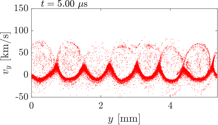
(b) $u_{zi0}=10$ km/s

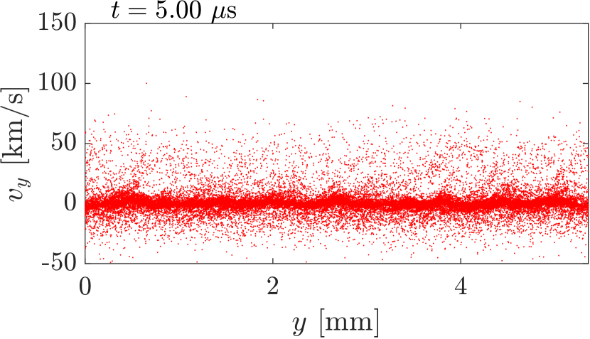
(c) $u_{zi0}=25$ km/s

Figure 16: Finite plasma with axial injection. Late behavior (at $t=5\mu$s) in the phase space plane $(y,v_{y})$ of ion particles contained in the axial slab $0.7\leq z/L_{z}\leq 0.75$.

For the fully periodic case, equation (13) shows that the evolution of total energy in the domain is fed by the equilibrium electric field $E_{0}$ and is tied to the presence of an average $j_{ze}$. Therefore, an energetically stationary state does not allow for an axial electron current. This theoretical conclusion is retrieved in our periodic simulations.

Axial injection and removal of particles involve energy inputs and losses through axial boundaries that have to be accounted for in the energy balance, yielding

$$\frac{\textmd{d}\mathcal{E}}{\textmd{d}t}=E_{0}\langle j_{ze}\rangle\mathcal{V}-P_{\textmd{out}},$$ (15)

where $P_{\textmd{out}}$ gathers the net energy outflow through axial boundaries and can be computed from the energies of removed and injected particles. The new term opens the possibility to have a balance between the energy input by $E_{0}$ and boundary losses, allowing for an energetically stationary behavior and an average $j_{ze}$ at the same time. Any energy loss term, such as inelastic collisions, could play a similar role in the balance.

The different terms in the balance equation (15) are computed and represented in figure 13 for the case with $u_{zi0}=10$ km/s, in the intermediate regime with a net $j_{ze}$. The balance is approximately fulfilled and the energy is close to stationary. There is, however, small changes in the total energy as well as in the partial energies of ions and electrons. The losses introduced by the axial boundary conditions limit enormously the heating that was observed in the fully periodic cases without losses. Actually, the total and species energies remain within levels close to the initial population. The electrostatic energy is, again, a minor contribution to the total energy.

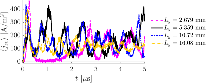
(a)

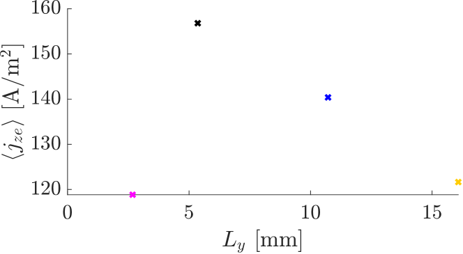
(b)

Figure 17: Finite plasma with axial injection. (a) Time evolution of the volume-averaged electron axial current $\left\langle j_{ze}\right\rangle$ for several $L_{y}$ and (b) its time average for $t\geq 2$ $\mu$s.

V Conclusions

The first part of this article is focused on the simulation of the classical ECDI with the PIC formulation and settings as close as possible to the linear kinetic theory. Unstable short-wavelength modes are seen to grow in the initially homogeneous plasma that fit qualitatively well the features of the theoretical ECDI dispersion relation in early simulation times. Close to saturation, some parts of the Fourier spectra show similarities with ion-acoustic modes. After saturation, the short scale modes vanish and the plasma tends to a new equilibrium with mild or long-wavelength oscillations and much more mode mixing. It is only during the growth and saturation of the ECDI modes that a turbulence-based axial current is induced in the electrons. The initial growth and saturation are related with the ion distribution that yields the characteristic vortex-like structure in phase space. The vanishing of oscillations seemed related with the blurring of those vortexes.

This behavior differs from the unlimited growth reported in the literature of 1D ECDI simulations with no virtual axial length [25, 22, 29], where the quenching of short modes was not seen. It is possible that the evolution we observe is not inherent to every ECDI simulation and depends on the choice of parameters. Other possibility is that more simulation time is needed in these works to reproduce the full behavior reported here, which is in line with our parametric analysis on the ion mass.

When axial boundaries are replaced by removal/injection surfaces, the refreshing of particles (mimicking the finite plasma in a Hall discharge) can yield completely different behaviors. These boundary conditions imply that particles that have interacted with the electrostatic wave are removed from the simulation eventually and new particles with the original distribution are injected. A key parameter is the ion injection velocity $u_{zi0}$, while its effect is negligible in the ECDI dispersion relation and periodic simulations. The intermediate regime where saturation and ion-residence times are similar is the only one yielding long-term short-scale oscillations and a turbulent-based axial current, and it is the most interesting one in the context of Hall discharges. A rough estimation with typical magnitudes shows that the condition for this regime is likely to happen in a conventional Hall thruster discharge.

References

- Choueiri and Ziemer [2001] E. Choueiri and J. Ziemer, Quasi-steady magnetoplasmadynamic thruster performance database, Journal of Propulsion and Power 17, 967 (2001).
- Ellison et al. [2012] C. Ellison, Y. Raitses, and N. Fisch, Cross-field electron transport induced by a rotating spoke in a cylindrical Hall thruster, Physics of Plasmas 19, 013503 (2012).
- MacDonald et al. [2011] N. A. MacDonald, M. A. Cappelli, S. R. Gildea, M. Martinez-Sanchez, and W. A. Hargus Jr, Laser-induced fluorescence velocity measurements of a diverging cusped-field thruster, Journal of Physics D: Applied Physics 44, 295203 (2011).
- Tsikata et al. [2009] S. Tsikata, N. Lemoine, V. Pisarev, and D. Gresillon, Dispersion relations of electron density fluctuations in a Hall thruster plasma, observed by collective light scattering, Physics of Plasmas 16, 033506 (2009).
- Tsikata and Minea [2015] S. Tsikata and T. Minea, Modulated electron cyclotron drift instability in a high-power pulsed magnetron discharge, Physical Review Letters 114, 185001 (2015).
- Tsikata et al. [2017] S. Tsikata, A. Héron, and C. Honoré, Hall thruster microturbulence under conditions of modified electron wall emission, Physics of Plasmas 24, 053519 (2017).
- Janes and Lowder [1966] G. Janes and R. Lowder, Anomalous electron diffusion and ion acceleration in a low-density plasma, Physics of Fluids 9, 1115 (1966).
- Bello-Benítez and Ahedo [2021] E. Bello-Benítez and E. Ahedo, Axial-azimuthal, high-frequency modes from global linear-stability model of a Hall thruster, Plasma Sources Science and Technology 30, 035003 (2021).
- Ramos et al. [2021] J. J. Ramos, E. Bello-Benítez, and E. Ahedo, Local analysis of electrostatic modes in a two-fluid E x B plasma, Physics of Plasmas 28, 052115 (2021).
- Koshkarov et al. [2019] O. Koshkarov, A. Smolyakov, Y. Raitses, and I. Kaganovich, Self-organization, structures, and anomalous transport in turbulent partially magnetized plasmas with crossed electric and magnetic fields, Physical Review Letters 122, 185001 (2019).
- Frias et al. [2012] W. Frias, A. Smolyakov, I. Kaganovich, and Y. Raitses, Long wavelength gradient drift instability in Hall plasma devices. I. Fluid theory, Physics of Plasmas 19, 072112 (2012).
- Nikitin et al. [2017] V. Nikitin, D. Tomilin, A. Lovtsov, and A. Tarasov, Gradient-drift and resistive mechanisms of the anomalous electron transport in Hall effect thrusters, Europhysics Letters 117, 45001 (2017).
- Sorokina et al. [2019] E. A. Sorokina, N. A. Marusov, V. P. Lakhin, and V. I. Ilgisonis, Discharge oscillations in Morozov’s stationary plasma thruster as a manifestation of large-scale modes of gradient drift instability, Plasma Physics Reports 45, 1 (2019).
- Romadanov et al. [2016] I. Romadanov, A. Smolyakov, Y. Raitses, I. Kaganovich, T. Tian, and S. Ryzhkov, Structure of nonlocal gradient-drift instabilities in hall exb discharges, Physics of Plasmas 23, 122111 (2016).
- Forslund et al. [1970] D. Forslund, R. Morse, and C. Nielson, Electron cyclotron drift instability, Physical Review Letters 25, 1266 (1970).
- Wong [1970] H. Wong, Electrostatic electron-ion streaming instability, Physics of Fluids 13, 757 (1970).
- Adam et al. [2004] J. Adam, A. Herón, and G. Laval, Study of stationary plasma thrusters using two-dimensional fully kinetic simulations, Physics of Plasmas 11, 295 (2004).
- Ducrocq et al. [2006] A. Ducrocq, J. Adam, A. Héron, and G. Laval, High-frequency electron drift instability in the cross-field configuration of Hall thrusters, Physics of Plasmas 13, 102111 (2006).
- Cavalier et al. [2013] J. Cavalier, N. Lemoine, G. Bonhomme, S. Tsikata, C. Honoré, and D. Grésillon, Hall thruster plasma fluctuations identified as the exb electron drift instability: Modeling and fitting on experimental data, PoP 20, 082107 (2013).
- Lafleur et al. [2016a] T. Lafleur, S. Baalrud, and P. Chabert, Theory for the anomalous electron transport in Hall effect thrusters. ii. kinetic model, Physics of Plasmas 23, 053503 (2016a).
- Janhunen et al. [2018a] S. Janhunen, A. Smolyakov, D. Sydorenko, M. Jimenez, I. Kaganovich, and Y. Raitses, Evolution of the electron cyclotron drift instability in two-dimensions, Physics of Plasmas 25, 082308 (2018a).
- Lafleur et al. [2016b] T. Lafleur, S. Baalrud, and P. Chabert, Theory for the anomalous electron transport in hall effect thrusters. i. insights from particle-in-cell simulations, Physics of Plasmas 23, 053502 (2016b).
- Lafleur and Chabert [2017] T. Lafleur and P. Chabert, The role of instability-enhanced friction on ‘anomalous’ electron and ion transport in Hall-effect thrusters, Plasma Sources Science and Technology 27, 015003 (2017).
- Coche and Garrigues [2014] P. Coche and L. Garrigues, A two-dimensional (azimuthal-axial) particle-in-cell model of a hall thruster, Physics of Plasmas 21, 023503 (2014).
- Janhunen et al. [2018b] S. Janhunen, A. Smolyakov, O. Chapurin, D. Sydorenko, I. Kaganovich, and Y. Raitses, Nonlinear structures and anomalous transport in partially magnetized ExB plasmas, Physics of Plasmas 25, 11608 (2018b).
- Asadi et al. [2019] Z. Asadi, F. Taccogna, and M. Sharifian, Numerical study of electron cyclotron drift instability: Application to hall thruster, Frontiers in Physics 7, 10.3389/fphy.2019.00140 (2019).
- Adam et al. [2008] J. Adam, J. Boeuf, N. Dubuit, M. Dudeck, L. Garrigues, D. Gresillon, A. Heron, G. Hagelaar, V. Kulaev, N. Lemoine, et al., Physics, simulation and diagnostics of Hall effect thrusters, Plasma Physics and Controlled Fusion 50, 124041 (2008).
- Charoy et al. [2019] T. Charoy, J. P. Boeuf, A. Bourdon, J. A. Carlsson, P. Chabert, B. Cuenot, D. Eremin, L. Garrigues, K. Hara, I. D. Kaganovich, A. T. Powis, A. Smolyakov, D. Sydorenko, A. Tavant, O. Vermorel, and W. Villafana, 2d axial-azimuthal particle-in-cell benchmark for low-temperature partially magnetized plasmas, Plasma Sources Science and Technology 28, 105010 (2019).
- Tavassoli et al. [2023] A. Tavassoli, M. Papahn Zadeh, A. Smolyakov, M. Shoucri, and R. J. Spiteri, The electron cyclotron drift instability: A comparison of particle-in-cell and continuum Vlasov simulations, Physics of Plasmas 30, 10.1063/5.0134457 (2023), 033905.
- Swanson [2003] D. Swanson, Plasma Waves, 2nd Edition (IOP Publishing, Bristol, UK, 2003).
- Frigo and Johnson [2005] M. Frigo and S. G. Johnson, The design and implementation of FFTW3, Proceedings of the IEEE 93, 216 (2005).
- Tavassoli et al. [2021] A. Tavassoli, O. Chapurin, M. Jimenez, M. Papahn Zadeh, T. Zintel, M. Sengupta, L. Couëdel, R. J. Spiteri, M. Shoucri, and A. Smolyakov, The role of noise in pic and Vlasov simulations of the Buneman instability, Physics of Plasmas 28, 10.1063/5.0070482 (2021).
- Chen et al. [2024] L. Chen, Z.-C. Kan, W.-F. Gao, P. Duan, J.-Y. Chen, C.-Q. Tan, and Z.-J. Cui, Growth mechanism and characteristics of electron drift instability in Hall thruster with different propellant types, Chinese Physics B 33, 015203 (2024).
- Smolyakov et al. [2019] A. Smolyakov, T. Zintel, L. Couedel, D. Sydorenko, A. Umnov, E. Sorokina, and N. Marusov, Anomalous electron transport in one-dimensional electron cyclotron drift turbulence, Plasma Physics Reports 46 (2019).
- Bello-Benítez and Ahedo [2023] E. Bello-Benítez and E. Ahedo, Stationary axial model of the Hall thruster plasma discharge: electron azimuthal inertia and far plume effects, Plasma Sources Science and Technology 32, 115011 (2023).