Stable Inverse Reinforcement Learning: Policies from Control Lyapunov Landscapes

Abstract

Learning from expert demonstrations to flexibly program an autonomous system with complex behaviors or to predict an agent’s behavior is a powerful tool, especially in collaborative control settings. A common method to solve this problem is inverse reinforcement learning (IRL), where the observed agent, e.g., a human demonstrator, is assumed to behave according to the optimization of an intrinsic cost function that reflects its intent and informs its control actions. While the framework is expressive, it is also computationally demanding and generally lacks convergence guarantees. We therefore propose a novel, stability-certified IRL approach by reformulating the cost function inference problem to learning control Lyapunov functions (CLF) from demonstrations data. By additionally exploiting closed-form expressions for associated control policies, we are able to efficiently search the space of CLFs by observing the attractor landscape of the induced dynamics. For the construction of the inverse optimal CLFs, we use a Sum of Squares and formulate a convex optimization problem. We present a theoretical analysis of the optimality properties provided by the CLF and evaluate our approach using both simulated and real-world data.

Control Lyapunov function, Convex optimization, Learning from demonstrations, Inverse optimality, Inverse reinforcement learning, Sum of Squares

1 INTRODUCTION

With recent advances in robotic technologies, autonomous systems are increasingly deployed in new domains. Frequently, these applications include the operation in close proximity and collaboration with human users, such as rehabilitation robotics, manufacturing, and autonomous driving [1, 2, 3]. As the envisaged tasks and level of collaboration get more involved, the need to flexibly program expressive human behavior models arises. The concept of learning a task by observing human experts is referred to as learning from demonstration and imitation learning [4, 5] and provides multiple advantages that facilitate effective human-robot collaboration. First, programming complex behavior does not require intimate knowledge regarding the task but instead only demonstrations are necessary. Second, user-specific preferences can be integrated in a natural manner, since they are implicitly encoded through the demonstrations. Lastly, the resulting policies and trajectories are easily interpretable as human behavior is emulated [6].

Imitation learning is generally more involved than replicating the observed demonstrations exactly via a state to action mapping, since the inferred control policies should ideally generalize well to previously unseen states and unknown environments. One way to achieve the desired generalization properties is by means of inverse reinforcement learning (IRL) which is an indirect imitation learning method [7]. Here, the demonstrating agent is assumed to act optimally with respect to an intrinsic cost function. By exploiting this optimality assumption to model the agent, the imitation learning problem is reformulated to inferring the intrinsic cost function driving the agent’s actions from observed data [8]. Since the optimal control policy is determined by this cost function, inferring the cost is sufficient to describe the agent’s behavior completely. Employing the optimality principle in human motor control is neuroscientfically well justified [9, 10] and algorithmically convenient, since it facilitates the use of principled approaches from optimal control theory [11]. Moreover, the cost function constitutes a concise representation of an agent’s behavior and has been shown to generalize well to previously unobserved environments [12]. However, in general IRL suffers from the inherent ill-posedness of the inference problem as many cost functions may explain the data well [13]. While there exist principled approaches to address the ambiguity, such as margin-based [8, 14] or entropy-based optimizations [15, 16, 17], the solution space of potential cost functions remains large. Additionally, IRL methods need to repeatedly solve an optimal control problem in the inner-loop of each learning iteration to evaluate the current cost function parametrization, which is computationally expensive for the nonlinear, nonconvex case. To mitigate this issue, some state-of-the-art IRL methods [18, 19, 20] only solve the forward problem approximately, thereby trading-off computational efficiency and precision. Finally, convergence guarantees for the inferred control policies are typically only provided for the linear-quadratic case [21] or if stable solutions are designed manually [22] instead of performing the inference from data.

An alternative and widely used approach to learning by demonstrations is by means of dynamic movement primitives (DMP) [23, 24]. In the DMP framework, demonstrations are represented as a set of differential equation and the resulting, stable dynamical system is used to encode the observed human behavior through its attractor landscape [25]. Due to its grounding in dynamical system theory, strong convergence and robustness guarantees can be achieved, which are favorable during operations with humans. Moreover, the model inference can be performed in a computationally efficient manner. However, in contrast to IRL approaches, DMP methods do not recover a control policy but only provide a dynamical system from which trajectory plans are generated. Therefore, the convenient stability guarantees are limited to the simulated reproductions and are not straight-forwardly retained by a subsequent tracking controller that is required to realize the planned trajectory. Furthermore, since no optimality principle is applied in this framework, DMP methods typically lack the more generalizing model representation provided by an inferred cost function. While some recent approaches concurrently learn a task-oriented potential function, e.g., a Lyapunov-like function, which is used to stabilize the learned dynamical system [26, 27, 28], the stabilization is only performed virtually and the control law is not applicable to a physical plant.

Therefore, both the IRL and DMP framework solve the imitation learning task in fundamentally different ways, resulting in complementary advantages. In this work we propose an IRL approach that unifies the distinct, beneficial properties of both frameworks. In particular we reformulate the cost function inference problem to learning a Lyapunov-constrained value function approximation from data by exploiting analogies between optimal control theory and robust stabilization, i.e., inverse optimality [29, 30, 31]. By continuously evaluating the learned value function using a gradient-based stabilizing control law available in closed-form, we directly search over the space of stable, closed-loop dynamical systems that best replicate the observed demonstrations, thereby conceptually bridging the gap to the DMP paradigm. Preliminary results have appeared in [32], which presents a framework for the time-discrete case showing convergence of the closed-loop system trajectories to a neighborhood of the equilibrium for a compact state space using a kernel-based approximation. In contrast, this article expands the proposed framework to the time-continuous case and achieves global asymptotic convergence properties. Additionally, a convex optimization approach using sum-of-squares (SOS) is deployed to construct inverse optimal control Lyapunov functions (CLF) from data. Finally, this work presents a rigorous, theoretical analysis of the optimality gap resulting from the Lyapunov-based approximation and provides an extensive evaluation using both simulated and real-world data in a comparison to a state-of-the-art IRL and DMP algorithm.

1.1 Organization and Notation

The remainder of this paper is structured as follows: After formulating the considered problem in Section 2, the Lyapunov-constrained value function approximation is derived in Section 3. Following this, Section 4 investigates the construction of inverse optimal CLFs using SOS and the convexification of the resulting optimization problem. In Section 5 and Section 7 the proposed approach is evaluated using both a simulation and a comparison study with real-world, human-generated data. Finally, we present our conclusion in Section 7.

Notation: Lower and upper case bold symbols denote vectors and matrices. $\mathbb{R}$ / $\mathbb{N}$ denote the set of all real/integer numbers respectively, while $\mathbb{R}_{+}$ / $\mathbb{N}_{+}$ denote all real/integer positive numbers. $\bm{I}_{n}$ is the $n\times n$ identity matrix. If a matrix $\bm{A}$ is positive definite, we write $\bm{A}\succ\bm{0}$, and $\bm{A}\succeq\bm{0}$ for positive semidefinitness. $\sqrt{\cdot}$ applied to a matrix means it is applied element-wise. $\pazocal{C}$ denotes the set of continuous functions, while $\pazocal{S}$ denotes the set of sum of squares decomposable polynomial functions. $\lfloor\cdot\rfloor$ and $\lceil\cdot\rceil$ denote the lowest and highest degrees of a polynomial’s monomials respectively. When applied to a vector of polynomials, $\lfloor\cdot\rfloor$ indicates the minimum and $\lceil\cdot\rceil$ the maximum over the degrees of all elements.

2 Problem Formulation

Consider a continuous-time, control-affine system

$$\dot{\bm{x}}=\bm{f}(\bm{x})+\bm{g}(\bm{x})\bm{u},$$ (1)

with continuous states $\bm{x}\in\mathbb{R}^{n}$ and initial condition $\bm{x}_{0}~{}\in~{}\mathbb{R}^{n}$. The system dynamics are given by ${\bm{f}\colon\mathbb{R}^{n}\to\mathbb{R}^{n}}$ and ${\bm{g}\colon\mathbb{R}^{n}\to\mathbb{R}^{n\times m}}$, where $\bm{f(\cdot)}$ and $\bm{g(\cdot)}$ are smooth and (1) is controllable, and the agent acting on the system is assumed to perform continuous control actions $\bm{u}\in\mathbb{R}^{m}$. The system description (1) is not particular restrictive since the assumed control-affine structure holds for many dynamical system classes, such as Euler-Lagrange systems. The following assumption is made for the considered system:

Assumption 1:

The functions $\bm{f(\cdot)}$ and $\bm{g(\cdot)}$ are known.

This assumption is not too restrictive since in many application scenarios, e.g., physical human-robot interaction, an accurate dynamics model of the robotic system can either be obtained a-priori using identification techniques [33] or be imposed by appropriate control schemes [34].

In the following, we employ the optimality principle to describe the behavior of an expert agent. This means that the agent is assumed to choose control actions $\bm{u}$ according to an intrinsic cost function with the goal of minimizing the accumulated stage costs over time. Thus, the agent employs the optimal control policy

$$\bm{\pi}^{\ast}(\bm{x})= \operatorname*{argmin}_{\bm{\pi}\colon\pazocal{X}\to\pazocal{U}}~{}\int_{t=0}^{\infty}l(\bm{x}-\bm{x}^{\ast})+\bm{\pi}(\bm{x})^{\intercal}\bm{R}\bm{\pi}(\bm{x})\,dt$$ (2a)

$$\mathrm{such~{}that~{}}\dot{\bm{x}}=\bm{f}(\bm{x})+\bm{g}(\bm{x})\bm{\pi}(\bm{x}),$$ (2b)

where $l\colon\mathbb{R}^{n}\to\mathbb{R}_{+,0}$ is a positive definite function representing state costs and $\bm{R}\in\mathbb{R}^{m\times m}\succ\bm{0}$ is a positive definite matrix denoting the control costs. Due to the structure of $l(\cdot)$ and $\bm{R}$, it is guaranteed that the costs in (2a) are positive everywhere except at the target state $\bm{x}^{\ast}$, which we denote as a meaningful cost in the following according to [30].

Since human behavior is not deterministic in general, e.g., due to inattentiveness or motor noise [35], the agent’s control policy does not correspond exactly to the deterministic optimal policy. These unaccounted variations in the control actions can be modelled as random perturbations [15]. Thus, we consider the agent to perform the perturbed optimal control policy

$$\bm{u}dt=\tilde{\bm{\pi}}(\bm{x})dt\coloneqq\bm{\pi}^{\ast}\!(\bm{x})dt+d\bm{\omega},$$ (3)

where $\bm{\omega}$ is an m-dimensional Brownian motion with state-dependent covariance $\bm{\Sigma}(\bm{x})\in\mathbb{R}^{m\times m}$. Given the perturbed policy (3), the closed-loop dynamics are rendered stochastic

$$d\bm{x}=\bm{f}(\bm{x})+\bm{g}(\bm{x})\bm{\pi}^{\ast}(\bm{x})+\bm{\sigma}(\bm{x})d\xi.$$ (4)

with $\bm{\sigma}(\bm{x})\coloneqq\bm{g}(\bm{x})\sqrt{\bm{\Sigma}(\bm{x})}$, where $\xi$ indicates n-dimensional standard Brownian motion.

Assumption 2:

The variance $\bm{\Sigma}(\cdot)$ is known.

This assumption is in general not particularly restrictive, since $\bm{\Sigma}(\cdot)$ can be identified from data [36]. While optimal control attempts to solve the problem of finding the optimal policy (2a) given the stage costs $l(\cdot)$ and $\bm{R}$, IRL considers the inverse problem. Here, an expert agent demonstrates state-action pairs and the goal is to infer the unknown cost function under which the associated optimal control policy best explains the observations. In order to retrieve the cost function the following assumptions are made for the perturbed policy (3) and the closed-loop dynamics (4):

Assumption 3:

The agent performs a goal-directed task, where the goal is defined by a unique target state $\bm{x}^{\ast}\in\mathbb{R}^{n}$.

Assumption 4:

The variance in (4) vanishes at the target; $\lim_{\bm{x}\to\bm{x}^{\ast}}\bm{\Sigma}(\bm{x})=\bm{0}$, such that $\tilde{\bm{\pi}}(\bm{x}^{\ast})=\bm{\pi}^{\ast}\!(\bm{x}^{\ast})$.

3 does not pose a strong restriction, because many complex tasks can be achieved by an ordered execution of goal-directed motions [37]. Since the target is unique, $\bm{x}^{\ast}$ coincides with the minimization of the agent’s cost function. Moreover, 4 states intuitively that the agent acts more deterministically close to the target state, which is necessary for task completion according to 3. Therefore, any agent that successfully performs the task has to act on the system such that it asymptotically converges to the desired final state $\bm{x}^{\ast}$. This has to hold true regardless of the stochasticity due to random perturbations in (4). In order to formalize this property, we introduce the following concept of stability.

Definition 1 ([38]):

A system (1) has an asymptotically stable equilibrium $\bm{x}^{*}$ on the set $\pazocal{X}$ if

1. for all $d\!>\!0$, there exist $\delta\!>\!0$, $t_{0}\!\geq\!0$ such that $\left\lVert\bm{x}_{0}\!-\!\bm{x}^{*}\right\rVert\!<\!\delta$ implies $\left\lVert\bm{x}(t)\!-\!\bm{x}^{*}\right\rVert\!<\!d$, $\forall t\!\geq\!t_{0}.$

2. $\lim_{t\to\infty}\left\lVert\bm{x}(t)\!-\!\bm{x}^{*}\right\rVert\!=\!0$ for all $\bm{x}_{0}\in\pazocal{X}$.

If the conditions hold for all states, i.e., $\bm{x}_{0}\in\mathbb{R}^{n}$, the equilibrium $\bm{x}^{*}$ is globally asymptotically stable.

Since the task is defined by a unique target state $\bm{x}^{*}$ in 3 at which the policy is deterministic according to 4, stabilization properties can be imposed for the agent’s control policy without loss of generality.

Assumption 5:

The perturbed policy (3) renders the equilibrium $\bm{x}^{*}$ asymptotically stable.

In general 5 is non-restrictive, since human motion naturally preserves regularity properties [10]. In the following, we consider the target $\bm{x}^{*}$ to be the origin without loss of generality. Based on 3, 4 and 5, we consider the problem of determining the value function

$$V^{*}(\bm{x})\!=\!\!\int_{t_{0}}^{\infty}\!\!l(\bm{x}(t))\!+\!\bm{\pi}^{\ast}\!(\bm{x}(t))^{\intercal}\bm{R}\bm{\pi}^{\ast}\!(\bm{x}(t))dt,\enspace\bm{x}_{t_{0}}=\bm{x}$$ (5)

which is the minimum cost-to-go from the current state $\bm{x}$ when following the optimal policy $\bm{\pi}^{*}(\cdot)$. The value function $V^{*}(\cdot)$ is defined though the Hamilton-Jacobi-Bellman (HJB) equation [39]

$$\begin{split}\nabla_{x}^{\intercal}V^{*}(\bm{x})\bm{f(x)}-\frac{1}{2}\left\lVert\nabla_{x}^{\intercal}V^{*}(\bm{x})\bm{g}(\bm{x})\right\rVert_{\bm{R}^{-1}}+l(\bm{x})=0.\end{split}$$ (6)

Moreover, if there exists a continuously differentiable, positive definite solution to (6), the optimal feedback control policy $\bm{\pi}^{*}(\cdot)$ directly follows from $V^{*}(\cdot)$ as such [40]:

$$\bm{\pi}^{*}(\bm{x})=-\bm{R}^{-1}\bm{g}(\bm{x})^{\intercal}\nabla_{x}V^{*}(\bm{x}).$$ (7)

While solving the HJB (6) directly is in general not tractable [40], we can exploit the direct dependence of the optimal policy $\bm{\pi}^{*}(\cdot)$ on the value function $V^{*}(\cdot)$ in (7) to infer the value function from data. To this end, we use the demonstrations dataset

$$\pazocal{D}=\{\tau_{1},\dots,\tau_{N}\},\qquad\text{with}\enspace\tau_{n}=\{\bm{x}_{t}^{n}\}_{t=0}^{T}$$ (8)

and $T,N\in\mathbb{N}_{+}$, which encode the agent’s preferences. Since the demonstrated state transitions are inherently provided in sampling increments, the dataset is given in a time-discrete form. Together with 5, we formulate the value function inference as a constrained functional optimization problem

$$V^{*}= \operatorname*{argmax}_{V\scaleobj{.9}{\in}\,\pazocal{C}}P\{V\>|\>\pazocal{D}$$

$$\mathrm{such~{}that~{}}\eqref{eq:opt_feedback}\mathrm{~{}asymptotically~{}stabilizes~{}\eqref{eq:unc_dyn}}.$$ (9a)

In (9), we aim to maximize the posterior of $V(\cdot)$ by comparing the state-visitation probabilities of the closed-loop dynamical system under the associated optimal policy and stochastic perturbations with the observed state transitions in the dataset (8). By maximizing the posterior $P\{V\>|\>\pazocal{D}\}$ it is possible to include potentially available knowledge through a prior probability distribution. Thereby, the value function $V^{*}(\cdot)$, which generates a feedback control $\bm{\pi}^{*}(\cdot)$ according to (7), that best explains the demonstrations $\pazocal{D}$ is found. Since additionally 5 must hold true, the posterior maximization becomes a constrained functional optimization problem, with (9a) guaranteeing that the inferred optimal control policy ${\bm{\pi}^{*}(\cdot)}$ stabilizes the system.

3 Lyapunov-based stability-certified inverse reinforcement learning

In order to infer the value function $V^{\ast}(\cdot)$ from data, while also considering the stability constraint on the corresponding optimal policy ${\bm{\pi}}^{*}(\cdot)$, we exploit the inverse optimal relationship between value functions and CLFs in the following. This allows us to reformulate constraint (9a) as a Lyapunov constraint on the optimal value function in Section 3.1. By further considering the optimal value function as a control Lyapunov function and exploiting closed-form expressions for stabilizing control policies, we approximate the posterior maximization (9) in a closed-form in Section 3.2. Finally, the resulting optimality gap due to the CLF-based approximation of the value function is analyzed theoretically in Section 3.3.

3.1 Lyapunov-Constrained Optimization

Stability as introduced in Definition 1 and used in 5 is an asymptotic convergence property, which can be analyzed with tools from dynamical system theory. A practical method to ascertain the convergence property of a system, without solving the underlying dynamics equations, is by means of Lyapunov stability theory [41]. One of the major strengths of Lyapunov stability theory is the existence of converse theorems, i.e., under the assumption of stability, a Lyapunov function is guaranteed to exist [42]. We exploit this together with another property of Lyapunov functions, which stems from the link between stability and optimality. Namely, the so called inverse optimality property, which states that every Lyapunov function is also a value function for a meaningful optimal stabilization problem. We employ both of these properties to formulate the original problem (9) as a Lyapunov-constrained optimization problem, which is guaranteed to be feasible. This is shown in the following result.

Lemma 1:

The Lyapunov-constrained functional optimization problem

$$V^{*}= \operatorname*{argmax}_{V\scaleobj{.9}{\in}\,\pazocal{C}} P\{V\>|\>\pazocal{D}\},$$ (9ja)

s.t. $$\phantom{\pazocal{L}}V(\bm{x})\,\;>0,\enspace\forall\bm{x}\in\pazocal{X}\setminus\{\bm{x}^{*}\},$$ (9jb)

$$\phantom{\pazocal{L}}V(\bm{x}^{*})=0,\enspace$$ (9jc)

$$\pazocal{L}V(\bm{x})\,\;<0,\enspace\forall\bm{x}\in\pazocal{X}\setminus\{\bm{x}^{*}\},$$ (9jd)

is feasible, where

$$\begin{split}\pazocal{L}V(\bm{x})=\nabla_{x}V(\bm{x})&{}^{\intercal}\big{(}\bm{f}(\bm{x})+\bm{g}(\bm{x})\bm{\pi}^{\ast}(\bm{x})\big{)}\end{split}$$ (9k)

is the lie derivative $\pazocal{L}V$ of system (1) under policy $\bm{\pi}^{*}(\cdot)$.

Proof: According to 5 the optimal policy ${\bm{\pi}}^{*}(\cdot)$ asymptotically stabilizes system (1) in the sense of Definition 1. Therefore, the converse Lyapunov theorem guarantees the existence of a Lyapunov function satisfying the constraints (9jb) - (9jd) [43]. $\square$

Note that the introduction of Lyapunov stability constraints (9jb) - (9jd) does not pose a restriction to the solution space, since the inverse optimality property establishes that every CLF also resembles an optimal value function for some meaningful cost defined by $l(\cdot)$ and $\bm{R}$ in (5) [30]. Thus, due to the converse Lyapunov theorem and the inverse optimality property, limiting the search to the space of Lyapunov functions still allow to express different preferences of an agent with a stabilizing optimal policy as assumed in (9a).

3.2 Closed-Form Likelihood Expression

In the previous section a feasible expression for the stability constraint is derived, which demonstrated the Lyapunov function’s principle capability to constitute a solution to the considered functional optimization problem (9). In this section we deal with maximizing the posterior (9), thereby ensuring that the found Lyapunov function encodes the observed preferences of the demonstrator.

We follow a Bayesian approach, which directly leads to the proportional relationship

$$P\{V\>|\>\pazocal{D}\}\propto P\{\tau_{1},\ldots,\tau_{N}\>|\>V\}P\{V\},$$

where $P\{V\}$ denotes the prior probability distribution over value functions $V(\cdot)$, which is a design choice. Since the $N$ trajectories $\tau_{1},\ldots,\tau_{N}$ are generated independently using the perturbed optimal policy $\tilde{\bm{\pi}}(\cdot)$, they are conditionally independent given the optimal policy $\bm{\pi}^{\ast}(\cdot)$. Due to (7), the associated optimal policy is strictly dependent on $V(\cdot)$, which implies

$$P\{\tau_{1},\ldots,\tau_{N}\>|\>V\}=P\{\tau_{1}\>|\>V\}\cdots P\{\tau_{N}\>|\>V\}.$$

Similarly, observed states $\bm{x}_{t}^{n}$ along a trajectory $\tau_{n}$ are conditionally Markovian given the optimal policy $\bm{\pi}^{\ast}(\cdot)$. Thus, it follows by the same argument as before that

$$P\{\tau_{n}\>|\>V\}=P\{\bm{x}_{0}^{n}\>|\>V\}\prod_{t=1}^{T}P\{{\bm{x}}_{t}^{n}\>|\>V,\bm{x}_{t-1}^{n}\},$$

where $P\{\bm{x}_{0}\>|\>V\}=P\{\bm{x}_{0}\}$ is the prior initial state distribution. As this prior is independent of $V(\cdot)$, we have

$$P\{\tau_{n}\>|\>V\}\propto\prod_{t=1}^{T}P\{{\bm{x}}_{t}^{n}\>|\>V,\bm{x}_{t-1}^{n}\}.$$

Since the observed state trajectories are increments sampled from the stochastic process (4) with n-dimensional standard Brownian motion $\xi$, it follows that each discrete state-transition probability $P\{{\bm{x}}_{t}^{n}\>|\>V,\bm{x}_{t-1}^{n}\}$ is normally distributed and, using standard integration methods, a closed-form expression for the probabilities can be obtained.

$$P\{{\bm{x}}_{t}^{n}\>|\>V,\bm{x}_{t-1}^{n}\}=$$

$$\pazocal{N}\big{(}{\bm{x}}_{t}^{n}\>|\>\bm{x}_{t-1}^{n}\!+\!\scaleobj{.8}{\int_{0}^{\Delta t}}\bm{f}(\bm{x}_{t-1}^{n})+\bm{g}(\bm{x}_{t-1}^{n})\bm{\pi}^{\ast}(\bm{x}_{t-1}^{n})\,d\tau,$$

$$\hskip 113.81102pt\bm{g}(\bm{x}_{t-1}^{n})^{\intercal}\bm{\Sigma}(\bm{x}_{t-1}^{n})\bm{g}(\bm{x}_{t-1}^{n})\big{)},$$

where $\Delta t$ is the sampling time. By combining the above derived equalities, we obtain the log-likelihood

$$\!\log(P\{V\!\>|\>\pazocal{D}\})\propto\log(P\{V\})-\!\sum_{n\!=\!1}^{N}\sum_{t\!=\!1}^{T}(\bm{e}_{t}^{n})^{\intercal}\bm{\Gamma}^{n}_{t}\bm{e}_{t}^{n},\!$$ (9l)

where

$$\bm{e}_{t}^{n} \!=\!\bm{x}_{t}^{n}\!-\!\Big{[}\bm{x}_{t-1}^{n}\!+\!\scaleobj{.8}{\int_{0}^{\Delta t}}\!\!\bm{f}(\bm{x}_{t-1}^{n})\!+\!\bm{g}(\bm{x}_{t-1}^{n})\bm{\pi}^{\ast}(\bm{x}_{t-1}^{n})\,d\tau\Big{]}$$ (9m)

$$\bm{\Gamma}_{t}^{n} =\left(\bm{g}(\bm{x}_{t-1}^{n})^{\intercal}\,\bm{\Sigma}(\bm{x}_{t-1}^{n})\,\bm{g}(\bm{x}_{t-1}^{n})\right)^{-1}.$$ (9n)

The log-likelihood (9l) measures how well the perturbed optimal policy $\bm{\tilde{\pi}}(\cdot)$ approximates the observed demonstrations $\pazocal{D}$ of the agent. Thus, the optimal value function $V^{*}(\cdot)$ is retrieved, as the unperturbed optimal policy $\bm{\pi}^{*}(\cdot)$ in (9m) directly depends on $V(\cdot)$ due to (7). Thereby, the loss in (9l) is minimized by finding a Lyapunov candidate function $V(\cdot)$ with an associated optimal policy $\bm{\pi}^{*}(\cdot)$ (7) that generates closed-loop dynamics with a state-visitation probability similar to the observed demonstration trajectories $\tau_{1},\ldots,\tau_{N}$.

However, the likelihood maximization (9l) is done with respect to a finite demonstration dataset $\pazocal{D}$ and therefore may only locally reproduce the true, underlying value function. Thus, we denote the resulting estimated value function with $\hat{V}(\cdot)$ in the following. In contrast, the desired stabilization property (9a) of the associated control policy (7) must hold true for an uncountable, infinite set of states in $\pazocal{X}$ and is not limited to the finite set of observed data points $\pazocal{D}$. Therefore, while the optimal control policy $\bm{\pi}^{*}(\cdot)$ induced by the true, unknown value function $V^{*}(\cdot)$ renders the system asymptotically stable due to 5, this may generally not be true when applying control law (7) with an estimated value function $\hat{V}(\cdot)$. To overcome this, we make use of the fact that the estimated $\hat{V}(\cdot)$ is a Lyapunov function by design due to the constraints (9jb) - (9jd), from which two advantages follow. First, the existence of a CLF for a control-affine system, such as (1), implies the existence of an asymptotically stabilizing control law [44], which we will denote with $\hat{\bm{\pi}}(\bm{x})$ in the following. Secondly, it is possible to calculate such a stabilizing control law $\hat{\bm{\pi}}(\cdot)$ explicitly and in closed-form if the system dynamics and CLF are known [45]. In [46] a slight variation of the original formulation (Sontag’s formula [45]) is introduced

$$\hat{\bm{\pi}}(\bm{x})\!=\!\begin{cases}-\lambda(\bm{x})\bm{R}^{-1}\bm{g}(\bm{x})^{\intercal}\nabla_{x}V(\bm{x}),&\quad\bm{g}^{\intercal}\nabla_{x}V\neq 0\\ 0,&\quad\bm{g}^{\intercal}\nabla_{x}V=0\end{cases}$$ (9o)

where $\lambda(\bm{x})\colon\mathbb{R}^{n}\to\mathbb{R}_{+,0}$ is a state-dependent, positive and continuous scalar factor. While in this work we propose to consider $\lambda(\cdot)$ as a functional design parameter, thereby softening the coupling between optimal and stabilizing policy in favor of gaining additional freedom for the control design, there are also analytic constructions of the scaling factor [46]

$$\lambda(x)=\cfrac{\nabla_{x}^{\intercal}V\bm{f}\!+\!\sqrt{(\nabla_{x}^{\intercal}V\bm{f})^{2}+l(\bm{x})\big{(}\nabla_{x}^{\intercal}V\bm{g}\bm{g}^{\intercal}\nabla_{x}V\big{)}}}{\nabla_{x}^{\intercal}V\bm{g}\bm{g}^{\intercal}\nabla_{x}V},$$ (9p)

where we omit the dependency on $\bm{x}$ for $\bm{f}$, $\bm{g}$ and $V$ for improved readability. It is shown in [40] that the control formulation (9o) together with (9p) produces the optimal policy $\bm{\pi}^{*}(\cdot)$ exactly, if the CLF $V(\cdot)$ and value function $V^{*}(\cdot)$ have the same shape level sets, i.e., the only difference between their gradients is a state dependent, scalar proportional factor

$$\nabla_{x}V^{*}=\lambda(\bm{x})\nabla_{x}V,$$ (9q)

which can be seen by substituting (9q) into the HJB (6) and solving for $\lambda(\cdot)$. Intuitively, the stabilizing policy $\hat{\bm{\pi}}(\cdot)$ in (9o) is similar to the optimal policy $\bm{\pi}^{*}(\cdot)$ (7) in the sense that both follow the directional information provided by the gradient of a potential function, e.g., either the the CLF $V(\cdot)$ or value function $V^{*}(\cdot)$. Therefore, given a CLF $V(\cdot)$, employing control law (9o) stabilizes system (1), whilst an appropriate choice for the point-wise scaling $\lambda(\cdot)$ along the gradient descent direction of $V(\cdot)$ may additionally solve the HJB equation. Hence, instead of employing the relationship between the value function $V^{*}(\cdot)$ and optimal policy $\bm{\pi}^{*}(\cdot)$, we propose to utilize the stabilizing control law $\hat{\bm{\pi}}(\cdot)$, since the estimated $\hat{V}(\cdot)$ is already constrained to be a CLF.

Analogously to before, the CLF $\hat{V}(\cdot)$ is fitted by evaluating the incurred loss under the closed-form control law $\hat{\bm{\pi}}(\cdot)$

$$\!\log(P\{\hat{V}\!\>|\>\pazocal{D}\})\mathrel{\vbox{ \offinterlineskip\halign{\hfil$#$\cr\propto\cr\kern 2.0pt\cr\sim\cr\kern-2.0pt\cr}}}\log(P\{\hat{V}\})-\!\sum_{n\!=\!1}^{N}\sum_{t\!=\!1}^{T}(\hat{\bm{e}}_{t}^{n})^{\intercal}\bm{\Gamma}^{n}_{t}\hat{\bm{e}}_{t}^{n},\!$$ (9t)

where

$$\bm{e}_{t}^{n} \!=\!\bm{x}_{t}^{n}\!-\!\Big{[}\bm{x}_{t-1}^{n}\!+\!\scaleobj{.8}{\int_{0}^{\Delta t}}\!\!\bm{f}(\bm{x}_{t-1}^{n})\!+\!\bm{g}(\bm{x}_{t-1}^{n})\hat{\bm{\pi}}(\bm{x}_{t-1}^{n})\,d\tau\Big{]}$$ (9u)

This approximate log-likelihood allows to infer ${V^{*}}(\cdot)$ indirectly by fitting a policy, merely substituting the optimal policy $\bm{\pi}^{*}(\cdot)$ by the stabilizing policy $\hat{\bm{\pi}}(\cdot)$. Thereby the proposed optimization (9t) still yields an estimate $\hat{V}(\cdot)$, which reflects the agent’s preferences, since the associated stabilizing policy $\hat{\bm{\pi}}(\cdot)$ best possibly represents the observed demonstrations, even though $\hat{V}(\cdot)$ is not an optimal value function in general.

3.3 Inverse Optimal Value Function Approximation

In this section we perform a theoretical analysis of the optimality gap resulting due to the approximation of $V^{*}(\cdot)$ using the CLF $\hat{V}(\cdot)$. Recall that the observed agent is modelled using the optimality principle, i.e., there exists an intrinsic cost function (2a) that the agent minimizes by employing the optimal policy $\bm{\pi}^{*}(\cdot)$. The value function $V^{*}(\cdot)$, that we attempt to infer in (9), represents an optimal aggregate of the costs experienced by the agent starting in any current state to the goal state. Thus, substituting the value function $V^{*}(\cdot)$ with the CLF-based approximation $\hat{V}(\cdot)$ also influences the underlying cost function that is being minimized by the associated policy $\hat{\bm{\pi}}(\cdot)$ and thereby impacts the representation of the modelled agent.

To theoretically analyze the implications of employing the CLF $\hat{V}(\cdot)$ and stabilizing policy $\hat{\bm{\pi}}(\cdot)$, we insert the state-dependent scaling factor $\lambda(\cdot)$ according to (9p). For notational convenience we let

$$a(\bm{x})=\nabla_{x}^{\intercal}\hat{V}(\bm{x})\bm{f}(\bm{x}),$$ (9v)

and

$$b(\bm{x})=\left\lVert\nabla_{x}^{\intercal}\hat{V}(\bm{x})\bm{g}(\bm{x})\right\rVert_{\bm{R}^{-1}},$$ (9w)

and introduce the slightly modified scaling function

$$\lambda(\bm{x})=\frac{a(\bm{x})+\sqrt{a(\bm{x})^{2}+2b(\bm{x})l(\bm{x})}}{b(\bm{x})}.$$ (9x)

When employing the CLF-based approximation to model the agent, the policy $\hat{\bm{\pi}}(\cdot)$ induced by the CLF $\hat{V}(\cdot)$ may not constitute an optimal minimizer for the cost function (2a) in general. However, the proposed formulation still retains a strong connection to the original optimal control problem (2), which is shown in the following result.

Theorem 1:

Consider a control-affine system as in (1) and a CLF-based value function estimate $\hat{V}(\cdot)$. Then applying control policy $\hat{\bm{\pi}}(\cdot)$ (9o) with scaling factor $\lambda(\cdot)$ according to (9x) solves the modified optimal control problem

$$\hat{\bm{\pi}}(\bm{x})= \operatorname*{argmin}_{\bm{\pi}\colon\pazocal{X}\to\pazocal{U}}~{}~{}\int_{t=0}^{\infty}\hat{l}(\bm{x})+\hat{r}(\bm{x},\bm{\pi(\bm{x})})\,dt$$ (9ya)

$$\mathrm{such~{}that~{}}\dot{\bm{x}}=\bm{f}(\bm{x})+\bm{g}(\bm{x})\bm{\pi}(\bm{x}),$$ (9yb)

with the meaningful cost functionals

$$\hat{l}(\bm{x})=\frac{1}{2}\lambda(\bm{x})b(\bm{x})-a(\bm{x}),$$ (9z)

and

$$\hat{r}(\bm{x})=\frac{1}{\lambda(\bm{x})}\bm{\pi}(\bm{x})^{\intercal}\bm{R}\bm{\pi}(\bm{x}).$$ (9aa)

Further, if $\hat{V}(\cdot)$ and $V^{*}(\cdot)$ have the same shape level sets (9q), the modified optimal control problem (9y) is similar to the original problem (2) in the sense that the relation

$$\hat{l}(\bm{x})r(\bm{x})=l(\bm{x})\hat{r}(\bm{x}),$$ (9ab)

where $r(\bm{x})=\bm{\pi}(\bm{x})^{\intercal}\bm{R}\bm{\pi}(\bm{x})$ denotes the original control costs in (2a), holds true.

Proof: In order to show that $\hat{\bm{\pi}}(\cdot)$ solves the modified optimal control problem (9y), we insert (9z) in the HJB

$$\begin{split}\nabla_{x}^{\intercal}V^{*}(\bm{x})\bm{f}(\bm{x})\!-\!\frac{\lambda(\bm{x})}{2}\!&\left\lVert\nabla_{x}^{\intercal}V^{*}(\bm{x})\bm{g}(\bm{x})\right\rVert_{\bm{R}^{-1}}\!\!\\ &\qquad+\!\frac{\lambda(\bm{x})}{2}b(\bm{x})\!-\!a(\bm{x})\!=\!0.\end{split}$$ (9ac)

With (9v) and (9w), it can be seen that the equality (9ac) holds, thereby showing that $\hat{\bm{\pi}}(\cdot)$ is the optimal policy for problem (9y). For $\hat{l}(\cdot)$ and $\hat{r}(\cdot)$ to constitute a meaningful cost, it remains to prove their positive definiteness. Since both $b(\cdot)$ and $l(\cdot)$ are positive definite it follows directly that

$$\sqrt{a(\bm{x})^{2}+2b(\bm{x})l(\bm{x})}\geq a(\bm{x}),\quad\forall x\in\mathbb{R}^{n},$$ (9ad)

when taking only the positive square root. This directly implies that $\lambda(\cdot)$ is positive definite according to (9x). Together with $\bm{R}\succ\bm{0}$ it follows that $\hat{r}(\cdot)$ in (9aa) is positive definite. Now inserting (9x) into (9z) we get

$$\hat{l}(\bm{x})=\frac{\sqrt{a(\bm{x})^{2}+2b(\bm{x})l(\bm{x})}-a(\bm{x})}{2},$$ (9ae)

which is also positive definite due to (9ad). Therefore, the modified optimal control problem (9y) has a meaningful cost function and the inverse optimality property holds.

For the second part, it remains to demonstrate that (9ab) is true. By inserting (9z) and (9aa) and writing out $r(\cdot)$ we obtain

$$\Big{(}\frac{1}{2}\lambda(\bm{x})^{2}b(\bm{x})\!-\!\lambda(\bm{x})a(\bm{x})\!-\!l(\bm{x})\Big{)}\frac{1}{2\lambda(\bm{x})}\bm{\pi}(\bm{x})^{\intercal}\bm{R}\bm{\pi}(\bm{x}) =0,$$

which holds true for $\lambda(\cdot)$ satisfying

$$\frac{1}{2}\lambda(\bm{x})^{2}b(\bm{x})-\lambda(\bm{x})a(\bm{x})-l(\bm{x})=0.$$ (9af)

If the CLF $\hat{V}(\cdot)$ and value function $V^{*}(\cdot)$ have co-linear gradients, we can rewrite the HJB (6) in terms of $\lambda(\bm{x})\nabla_{x}\hat{V}(\cdot)$ such that

$$\begin{split}\lambda(\bm{x})\nabla_{x}^{\intercal}\hat{V}(\bm{x})\bm{f}(\bm{x})-\frac{1}{2}\lambda(\bm{x})^{2}&\left\lVert\nabla_{x}^{\intercal}\hat{V}(\bm{x})\bm{g}(\bm{x})\right\rVert_{\bm{R}^{-1}}\\ &\qquad\qquad+l(\bm{x})=0.\end{split}$$ (9ag)

Thus, given the definition of $a(\cdot)$ (9v) and $b(\cdot)$ (9w), it follows from (9ag) that equality (9af) holds true, which concludes the proof. $\square$

Intuitively, the similarity (9ab) in Theorem 1 indicates that the proposed approximation via the CLF $\hat{V}(\cdot)$ and stabilizing policy $\hat{\bm{\pi}}(\cdot)$ weights the state and control costs proportionally in the same way as in the original optimal control problem (2). Another way to interpret this correspondence is that the modified optimal control problem (9y) modulates the stage costs of the original optimal control problem (2) using $\lambda(\cdot)$:

$$\hat{\bm{\pi}}(\bm{x})=\operatorname*{argmin}_{\bm{\pi}\colon\pazocal{X}\to\pazocal{U}}~{}~{}\int_{t=0}^{\infty}\frac{1}{\lambda(\bm{x})}\big{(}l(\bm{x})+r(\bm{x})\big{)}\,dt,$$

which can be seen by multiplying $\hat{l}(\cdot)$ (9z) and $\hat{r}(\cdot)$ (9aa) with $\lambda(\cdot)$ and solving the equations using (9x).

4 Sum of Squared based Lyapunov formulation

While the formulation in (9j) together with the approximate log-likelihood (9t) provides an appealing framework for the inference of $V^{*}(\cdot)$, it requires solving a functional optimization problem. Therefore, expressive function approximators are needed. Thus, in this section we employ the sum of squares (SOS) technique and transform (9j) into a constrained optimization over the space of polynomials. In Section 4.1 we rewrite the functional optimization (9j) into an SOS program and introduce Lyapunov constraints in Section 4.2. Finally, we propose a convexification scheme in Section 4.3 to create tractable SDPs for the Lyapunov-constrained optimization.

4.1 Formulation as SOS Program

The SOS technique is an efficient approach to test whether a given polynomial is non-negative by checking if it can be expressed as a sum of squares. Since the Lyapunov constraints (9jb) - (9jd) are also positive-definiteness conditions, they can conveniently be expressed as SOS constraints [47]. To this end, we parameterize $\hat{V}(\cdot)$ as a multivariate polynomial consisting of monomial vector $\bm{z}(\bm{x})$ and real scalar coefficients $\bm{c}$

$$\hat{V}(\bm{c},\bm{x})=\bm{c}^{\intercal}\bm{z}(\bm{x}),$$ (9ah)

which is not particularly restrictive since polynomials are known to be sufficiently expressive to approximate a large family of functions [48]. Due to (9ah), the stabilizing control law $\hat{\bm{\pi}}(\cdot)$ becomes

$$\hat{\bm{\pi}}(\bm{c},\bm{x})\!=\!\begin{cases}-\lambda(\bm{x})\bm{R}^{-1}\bm{g}^{\intercal}\nabla_{x}\bm{z}(\bm{x})^{\intercal}\bm{c},&\enspace\bm{g}^{\intercal}\nabla_{x}\bm{z}\!\neq\!0\\ 0,&\enspace\bm{g}^{\intercal}\nabla_{x}\bm{z}\!=\!0,\end{cases}$$ (9ai)

which has a linear dependence on $\bm{c}$. Thus, the empirical error (9u) admits a representation that is linear in $\bm{c}$ as well

$$\begin{split}\hat{\bm{e}}_{t+1}^{n}(\bm{c})=\bm{x}&{}_{t+1}^{n}\!-\!\bm{x}_{t}^{n}\\ &\!+\!\scaleobj{.8}{\int_{0}^{\Delta t}}\!\!\bm{f}(\bm{x}_{t}^{n})\!+\!\lambda(\bm{x}_{t}^{n})\!\left\lVert\bm{g}(\bm{x}_{t}^{n})\right\rVert_{\bm{R}^{-1}}\!\!\nabla_{x}^{\intercal}\bm{z}(\bm{x}_{t}^{n})\bm{c}\,d\tau\end{split}$$

Moreover, since the posterior optimization (9t) reduces to a search over the coefficients $\bm{c}$, the prior $P(\hat{V})$ in (9t) can be defined in terms of $\bm{c}$ as well. We choose a multivariate, zero-mean normal distribution ${\bm{c}\sim\pazocal{N}(\bm{0},\bm{\Sigma}_{c})}$, which yields a closed-form expression for the parameterized log-likelihood

$$\!\log(P\{\hat{V}\!\>|\>\pazocal{D}\})\!\mathrel{\vbox{ \offinterlineskip\halign{\hfil$#$\cr\propto\cr\kern 2.0pt\cr\sim\cr\kern-2.0pt\cr}}}\!-\frac{1}{2}\bm{c}^{\intercal}\bm{\Sigma}_{c}^{-1}\bm{c}-\sum_{n\!=\!1}^{N}\sum_{t\!=\!1}^{T}\hat{\bm{e}}_{t}^{n}(\bm{c})^{\intercal}\bm{\Gamma}^{n}_{t}\hat{\bm{e}}_{t}^{n}(\bm{c}).\!$$ (9al)

The parameterized log-likelihood (9al) contains terms that are quadratic in $\bm{c}$ and can therefore not be used directly in a convex SDP problem. However, using the epigraph formulation, (9al) is reformulated to be linear in the decision variables.

Lemma 2:

Consider a control-affine system (1), a dataset $\pazocal{D}$ as in (8), a control law $\bm{\hat{\pi}}(\bm{c},\bm{x})$ according to (9ai) and the scalar variables $q,p\in\mathbb{R}$. Then maximizing the parameterized log-likelihood (9al) over $\pazocal{D}$ is equivalent to solving the SDP problem

$$\bm{c^{*}}= \operatorname*{argmin}_{\bm{c},q,p}\quad q+p$$ (9ama)

$$\text{ such that}\enspace\bm{Q}(q,\bm{c})\succeq 0,$$ (9amb)

$$\phantom{\text{ such that}}\enspace\bm{P}(p,\bm{c})\succeq 0,$$ (9amc)

where

$$\bm{P}(p,\bm{c}):= \begin{bmatrix}p&\bm{c}^{\intercal}\\ \bm{c}&\bm{\Sigma}_{c}\end{bmatrix}\in\mathbb{R}^{\binom{n+d_{m}}{d_{m}}\times\binom{n+d_{m}}{d_{m}}},$$ (9an)

$$\bm{Q}(q,\bm{c}):= \begin{bmatrix}q&\bm{\varepsilon}(\bm{c})\\ \bm{\varepsilon}(\bm{c})^{\intercal}&\bm{G}^{-1}\end{bmatrix}\in\mathbb{R}^{(1+nNt)\times(1+nNt)},$$ (9ao)

with

$$\bm{\varepsilon}(\bm{c}):= \big{[}(\hat{\bm{e}}_{1}^{1}(\bm{c}))^{\intercal}...(\hat{\bm{e}}_{t}^{n}(\bm{c}))^{\intercal}\big{]}\in\mathbb{R}^{1\times nNt}$$ (9ap)

$$\bm{G}:= \text{diag}\big{(}\bm{\Gamma}^{1}_{1},\ldots,\bm{\Gamma}^{n}_{t}\big{)}\in\mathbb{R}^{(nNt)\times(nNt)}.$$ (9aq)

Proof: We maximize (9al) by minimizing the regularized empirical error $\bm{\hat{e}}(\bm{c})$ over dataset $\pazocal{D}$

$$\bm{{c}^{*}}=\operatorname*{argmin}_{\bm{c}}\sum_{n\!=\!1}^{N}\sum_{t\!=\!1}^{T}\hat{\bm{e}}_{t}^{n}(\bm{c})^{\intercal}\bm{\Gamma}^{n}_{t}\hat{\bm{e}}_{t}^{n}(\bm{c})+\frac{1}{2}\bm{c}^{\intercal}\bm{\Sigma}_{c}^{-1}\bm{c}.$$ (9ar)

Using the epigraph reformulation [49], we equivalently transform (9ar) into a linear optimization problem with quadratic inequality constraints

$$\bm{c^{*}}= \operatorname*{argmin}_{\bm{c},q,p}\quad q+p$$ (9asa)

$$\text{ such that}\enspace\bm{\varepsilon}(\bm{c})\bm{G}\bm{\varepsilon}(\bm{c})^{\intercal}\leq q$$ (9asb)

$$\hskip 52.00005pt\frac{1}{2}\bm{c}^{\intercal}\bm{\Sigma}_{c}^{-1}\bm{c}\,\leq p,$$ (9asc)

where $q$ and $p$ are the newly introduced epigraph variables. Thus, it remains to reformulate (9asb) and (9asc) as LMI constraints to obtain an SDP. Due to the definition of $\bm{G}$, the properties $\text{det}(\bm{G})\neq 0$ and $\bm{G}=\bm{G}^{\intercal}$ hold and it follows from the Schur complement [50] that (9asb) is equivilant to

$$q-\bm{\varepsilon}(\bm{c})\bm{G}\bm{\varepsilon}(\bm{c})^{\intercal}\geq 0\iff\begin{bmatrix}q&\bm{\varepsilon}(\bm{c})\\ \bm{\varepsilon}(\bm{c})^{\intercal}&\bm{G}^{-1}\end{bmatrix}\succeq 0,$$ (9at)

where the positive semidefinite matrix on the right is exactly $\bm{Q}$ (9ao). Following the same procedure for (9asc), we obtain

$$p-\frac{1}{2}\bm{c}^{\intercal}\bm{\Sigma}_{c}^{-1}\bm{c}\geq 0\iff\begin{bmatrix}p&\bm{c}^{\intercal}\\ \bm{c}&\bm{\Sigma}_{c}\end{bmatrix}\succeq 0.$$ (9au)

Finally, substituting the quadratic constraints in (9as) with the right hand side of (9at) and (9au) yields the optimization problem (9am) and thus concludes the proof. $\square$

Solving SDP (9am) thus allows us to find a parameterization $\bm{c}^{*}$ such that the employed control law $\bm{\hat{\pi}}(\bm{c}^{*},\bm{x})$ reproduces the observed trajectories. Moreover, inferring $\bm{c}^{*}$ directly determines $\hat{V}(\bm{c}^{*},\bm{x})$ due to (9ah), thereby estimating the underlying value function as well. However, since the SDP problem (9am) in its current form does not entail the Lyapunov constraints (9jb) - (9jd), it is not ascertained that the retrieved $\hat{V}(\bm{c}^{*},\bm{x})$ is also a CLF and not guaranteed that the employed control law $\bm{\hat{\pi}}(\bm{c}^{*},\bm{x})$ asymptotically stabilizes system (1).

4.2 Lyapunov-Constrained Nonlinear SOS Program

Parameterizing $\hat{V}(\bm{c},\cdot)$ as a multivariate polynomial allows a straightforward extension to introduce the stability constraints (9jb) - (9jd) as SOS conditions. To this end, we impose the following assumption on the system dynamics (1).

Assumption 6:

The functions $\bm{f(\cdot)}$ and $\bm{g(\cdot)}$ in (1) are polynomial.

Due to 6 the derivative constraint (9jd) takes a polynomial form and can be expressed using the SOS technique. This is accomplished by decomposing the polynomial into a quadratic form and testing its decomposition matrix for positive semidefiniteness, which is formalized as follows:

Definition 2 ([51]):

We call a multivariate polynomial $p(\bm{x})$ of degree $2d$ (with $d\geq 1$) SOS decomposable if and only if there exists a positive semidefinite matrix $\bm{H}$ and a monomial vector $\bm{m}(\bm{x})$ of at least degree $d$ such that

$$p(\bm{x})=\bm{m}(\bm{x})^{\intercal}\bm{H}\bm{m}(\bm{x})\quad\text{ s.t. }\bm{H}\succeq 0$$ (9av)

Any polynomial $p(\bm{x})$ that is SOS decomposable is trivially non-negative. We will denote the set of all polynomials that fulfill Definition 2 with $\pazocal{S}$. Hence, $p(\bm{x})\in\pazocal{S}$ is equivalent to saying that $p(\bm{x})$ is non-negative. Since constraints (9jb) and (9jd) require strict positivity except at the equilibrium, we offset the Lyapunov conditions by a positive-definite polynomial

$$\hat{V}(\bm{c,x})-\mu(\bm{x}) \in\pazocal{S}$$ (9awa)

$$-\pazocal{L}\hat{V}(\bm{c,x})-\mu(\bm{x}) \in\pazocal{S},$$ (9awb)

with $\mu(\bm{x})>0,\;\forall\>\bm{x}\neq\bm{0}$. Since $\mu(\cdot)$ can in principle be chosen arbitrarily small, it poses a negligible restriction. A necessary condition for (9awa) and (9awb) to be SOS decomposable is that the smallest and largest degrees among all monomials in both constraints have to be even. Thus, the coefficients for the smallest and largest degrees among all monomials appearing in both constraints need to be dependent on $\bm{c}$. The following result shows under which conditions this is given.

Lemma 3:

Consider a control-affine system (1) satisfying 1 and 6, a parameterized polynomial function $\hat{V}(\bm{c},\bm{x})$ according to (9ah) and the resulting parametrized control law $\hat{\bm{\pi}}(\bm{c},\bm{x})$ (9ai). If the minimum-degree conditions

$$\lfloor\lambda(\bm{x})\rfloor\wedge\lfloor\bm{g}(\bm{x})\rfloor =0,$$ (9axa)

$$\lfloor\bm{f}(\bm{x})\rfloor \geq 1,$$ (9axb)

$$\lfloor\mu(\bm{x})\rfloor \geq\lfloor\hat{V}(\cdot,\bm{x})\rfloor=2,$$ (9axc)

and maximum-degree conditions

$$\qquad\lceil\hat{V}(\cdot,\bm{x})\rceil =2i\geq\lceil\mu(\bm{x})\rceil\wedge\lceil\bm{f}(\bm{x})\rceil,$$ (9aya)

$$\lceil\lambda(\bm{x})\rceil =2j$$ (9ayb)

with ${i,j\in\mathbb{N_{+}}}$ hold true, then the necessary degree conditions for (9aw) are satisfied.

Proof: Due to (9axc) and (9aya) it follows directly that the lowest and highest monomial degree in (9awa) are even and depend on the decision variables $\bm{c}$. Thus, it remains to verify the degree conditions for (9awb). Inserting policy (9ai) yields

$$-\nabla_{x}^{\intercal}\hat{V}(\bm{c},\bm{x})\bm{f}(\bm{x})\!\!+\!\!\lambda(\bm{x})\!\left\lVert\nabla_{x}^{\intercal}\hat{V}(\bm{c},\bm{x})\bm{g}(\bm{x})\right\rVert_{\bm{R}^{-1}}\!\!\!-\mu(\bm{x})\!\in\pazocal{S}.$$ (9az)

To verify the degree conditions, we show that the lowest and highest monomial degrees in (9az) are bounded by terms depending on $\hat{V}(\bm{c},\bm{x})$ and are even. The lowest monomial degree of each term in (9az) fulfills

$$\lfloor\lambda(\bm{x})\left\lVert\nabla_{x}^{\intercal}\hat{V}(\bm{c},\bm{x})\bm{g}(\bm{x})\right\rVert_{\bm{R}^{-1}}\rfloor =2$$ (9baa)

$$\lfloor-\nabla_{x}^{\intercal}\hat{V}(\bm{c},\bm{x})\bm{f}(\bm{x})\rfloor \geq 2$$ (9bab)

$$\lfloor-\mu(\bm{x})\rfloor \geq 2$$ (9bac)

Thus, due to (9baa), the lowest possible monomial degree in (9az) is even and depends on $\hat{V}(\bm{c},\bm{x})$. For the highest monomial degree in (9az), it can be seen that

$$\lceil\lambda(\bm{x})\!\left\lVert\nabla_{x}^{\intercal}\hat{V}(\bm{c},\bm{x})\bm{g}(\bm{x})\right\rVert_{\bm{R}^{-1}}\!\rceil \!\geq\!\lceil\!-\nabla_{x}^{\intercal}\hat{V}(\bm{c},\bm{x})\bm{f}(\bm{x})\rceil$$ (9bba)

$$\lceil\lambda(\bm{x})\!\left\lVert\nabla_{x}^{\intercal}\hat{V}(\bm{c},\bm{x})\bm{g}(\bm{x})\right\rVert_{\bm{R}^{-1}}\!\rceil \!\geq\!\lceil\mu(\bm{x})\rceil$$ (9bbb)

due to (9aya). Finally, inserting (9ayb) yields

$$\begin{split}\lceil\lambda(\bm{x})\!\left\lVert\nabla_{x}^{\intercal}\hat{V}(\bm{c},\bm{x})\bm{g}(\bm{x})\right\rVert_{\bm{R}^{-1}}\!\rceil\!=\!2(\lceil\hat{V}(\bm{c},\bm{x})\rceil\!\!-\!\!1\!\!+\!\!\lceil\bm{g}(\bm{x})\rceil\!\!+\!\!j),\end{split}$$

which can trivially be seen to be even. Hence, the highest monomial degree in (9az) is also guaranteed to be an even and dependent on $\hat{V}(\bm{c},\bm{x})$, which concludes the proof. $\square$

Intuitively, (9axb) ensures vanishing open-loop dynamics $\bm{f}(\cdot)$ at the equilibrium, while (9axa) restricts $\bm{g}(\cdot)$ and $\lambda(\cdot)$ to have non-vanishing control influence of $\nabla_{x}\hat{V}(\cdot)$ around the equilibrium. By combining the results of Lemma 2 and 3 we get the SOS-constrained optimization problem

$$\bm{c^{*}}= \operatorname*{argmin}_{\bm{c},q,p} q+p$$ (9bca)

such that $$\bm{Q}(q,\bm{c})\succeq 0,$$ (9bcb)

$$\bm{P}(p,\bm{c})\succeq 0,$$ (9bcc)

$$\hat{V}(\bm{c,x})-\mu(\bm{x})\in\pazocal{S},$$ (9bcd)

$$-\pazocal{L}\hat{V}(\bm{c,x})-\mu(\bm{x})\in\pazocal{S}.$$ (9bce)

Optimizing (9bc) over $\bm{c}$ yields an estimate $\hat{V}(\bm{c}^{*},\bm{x})$ that fulfills the Lyapunov constraints (9jb) - (9jd) while also encoding agent preferences through the parameterized log-likelihood (9al). Here, $\hat{V}(\bm{c}^{*},\bm{x})$ concurrently determines the policy $\bm{\hat{\pi}}(\bm{c}^{*},\bm{x})$ through its gradient $\nabla_{x}\hat{V}(\cdot)$ in (9ai), which is guaranteed to asymptotically stabilize system (1) due to the SOS constraints (9bcd) and (9bce). Thus, solving (9bc) constitutes an integrated certification and stabilization framework.

However, (9bce) remains a restriction preventing the direct implementation of (9bc) as a convex SDP problem, since the constraint is nonlinear in the decision variables $\bm{c}$. This can be seen when writing out (9bce) in the parameterized form

$$-\bm{c}\nabla_{x}^{\intercal}\bm{z}(\bm{x})\bm{f}(\bm{x})+\!\lambda(\bm{x})\!\left\lVert\bm{c}\nabla_{x}^{\intercal}\bm{z}(\bm{x})\bm{g}(\bm{x})\right\rVert_{\bm{R}^{-1}}\!-\!\mu(\bm{x})\!\in\!\pazocal{S},$$ (9bd)

where the second term is quadratic in $\bm{c}$, thereby yielding a quadratic matrix inequality (QMI). While some QMI define a convex solution set and allow an equivalent reformulation as an LMI [52], this not the case for (9bd), which is demonstrated in the following proposition.

Proposition 1:

The solution set of (9bd) is nonconvex and cannot be reformulated to an equivalent LMI constraint.

Proof: Consider the linear one dimensional system $f(x)=x$ with $g(x)=1$ and $x\in\mathbb{R}^{1}$. Further choose a quadratic Lyapunov candidate $V(c,x)=cx^{2}$. Then (9bd) becomes

$$-2cx\big{(}x-\lambda 2cx\big{)}-\mu(x)\in\pazocal{S},$$ (9be)

with a bounding polynomial $\mu(x):=wx^{2}$ for some small $1\gg w>0$. Thus, (9be) can be rewritten as

$$x\big{(}4\lambda c^{2}-2c-w\big{)}x\in\pazocal{S}.$$ (9bf)

It can be seen directly that the SOS condition holds true, if

$$4\lambda c^{2}-2c-w\geq 0.$$ (9bg)

Without loss of generality, choose $\lambda=\frac{1}{2}$ and exploit the fact that $w$ can be chosen arbitrarily close to $0$ to express (9bg) as a strict inequality

$$2c^{2}>2c.$$ (9bh)

It is straight forward to infer the solution set from (9bh) to

$$\{c\in\mathbb{R}\mid c>1\;\cup\;c<0\},$$ (9bi)

which is nonconvex, thereby concluding the proof by counter example. $\square$

Thus, the constrained optimization problem (9bc) requires solving a QMI due to (9bce). While there exist approaches to solve optimization problems with nonlinear matrix inequalities [53, 54, 55], they are typically prohibitively expensive for larger problems or alter the accompanying objective function. Therefore, in the following section we propose a procedure to solve (9bc) in a convex form.

4.3 Convexified Lyapunov-Constrained Optimization

If a QMI is bilinear [52], it can be solved efficiently using a convexification approach. In particular, the bilinear form can be exploited to reduce a QMI to a convex LMI by fixing one set of decision variables and optimizing over the remaining ones. Thus, optimizing alternately between the two parameter sets yields a sequence of convex SDPs [56]. However, employing this scheme directly to (9bc) is not possible, since the constraint (9bce) is not bilinear. To overcome this, we make use of the structure of the derivative constraint (9bd). In particular, under mild conditions it is always possible to find a feasible solution to the Lyapunov-constrained optimization (9bc) using a sufficiently large ${\lambda(\cdot)}$, which is demonstrated in the following.

Lemma 4:

Consider a control-affine, continuous system (1) satisfying the degree conditions of Lemma 3. If the set

$$\{\bm{x}\mid\bm{g}(\bm{x})=\bm{0},\nabla_{x}^{\intercal}V(\bm{x})\bm{f}(\bm{x})\geq 0,\bm{x}\neq\bm{0}\}$$ (9bj)

is empty and a Lyapunov function candidate $V(\bm{x})$ satisfying

$$V(\bm{x})>0,\quad\forall\bm{x}\neq\bm{0}$$ (9bk)

$$\nabla_{x}V(\bm{x})\neq\bm{0},\quad\forall\bm{x}\neq\bm{0}$$ (9bl)

is given, there always exists a continuous, positive definite $\lambda(\bm{x})$ that asymptotically stabilizes (1) under the stabilizing control policy $\bm{\hat{\pi}}(\bm{x})$ (9o).

Proof: Since $V(\cdot)$ is positive definite due to (9bk), it remains to show that $\dot{V}(\cdot)$ is negative definite. After inserting control law (9o) and rearranging we obtain

$$\lambda(\bm{x})\left\lVert\nabla_{x}^{\intercal}V(\bm{x})\bm{g}(\bm{x})\right\rVert_{\bm{R}^{-1}}>\nabla_{x}^{\intercal}V(\bm{x})\bm{f}(\bm{x})\quad\forall\bm{x}\neq\bm{0}$$ (9bm)

For any state with $\bm{g}(\bm{x})=\bm{0}$, the right hand side of (9bm) needs to be negative, which is guaranteed since the set (9bj) is empty. Otherwise, we can always choose a sufficiently large $\lambda(\bm{x})>0$ such that (9bm) is fulfilled, since the norm term on the left is guaranteed to be positive definite due to (9bl) and $\bm{R}$ being positive definite, which concludes the proof. $\square$

Intuitively, (9bj) requires that the system needs to be controllable in states where the stability constraints are violated by the open-loop dynamics, which is not particularly restrictive. Moreover, Lemma 4 states that a control policy that follows the direction of $\nabla_{x}V(\cdot)$ is guaranteed to exist and stabilize the system given a sufficiently large ${\lambda}(\cdot)$, if $V(\cdot)$ has a non-zero gradient everywhere except at the equilibrium. Therefore, we propose to substitute the derivative constraint (9bce) by imposing a non-zero gradient constraint (9bl) on $\hat{V}(\cdot,\cdot)$ and additionally optimize over ${\lambda}(\cdot)$. In order to avoid restricting the solution space unnecessarily, e.g., by enforcing convexity, we propose an iterative procedure, where the solution at each iteration $i$ is guaranteed to yield a $\hat{V}(\bm{c}_{i},\cdot)$ that satisfies the non-zero gradient condition (9bl).

Lemma 5:

Given a parameter vector $\bm{c}_{i}$ at iteration $i$ for which a polynomial $\hat{V}(\bm{c}_{i},\bm{x})$ of the form (9ah) satisfies

$$\nabla_{x}^{\intercal}\hat{V}(\bm{c}_{i},\bm{x})\nabla_{x}\hat{V}(\bm{c}_{i},\bm{x})>0,\quad\forall\bm{x}\neq\bm{0},$$ (9bn)

then solving the SOS-problem

$$\bm{c}_{i+1}=\text{find } \enspace\bm{c}$$ (9bo)

s.t. $$\;\nabla_{x}^{\intercal}\hat{V}(\bm{c}_{i},\bm{x})\nabla_{x}\hat{V}(\bm{c},\bm{x})-\mu(\bm{x})\in\pazocal{S},$$ (9bp)

at iteration $i\!+\!1$ yields a parameter vector $\bm{c}_{i+1}$ for which $\hat{V}(\bm{c}_{i+1},\bm{x})$ fulfills the non-zero gradient constraint (9bl).

Proof: Since $\mu(\bm{x})$ is positive definite, we get for (9bo)

$$\nabla_{x}^{\intercal}\hat{V}(\bm{c}_{i},\bm{x})\nabla_{x}\hat{V}(\bm{c}_{i+1},\bm{x})>0\quad\forall\bm{x}\neq\bm{0}.$$ (9bq)

Squaring both sides of (9bq) yields

$$\nabla_{x}^{\intercal}\hat{V}_{i}(\bm{x})\nabla_{x}\hat{V}_{i+1}(\bm{x})\nabla_{x}^{\intercal}\hat{V}_{i}(\bm{x})\nabla_{x}\hat{V}_{i+1}(\bm{x})>$$ (9br)

∀x≠0,

where $\hat{V}_{i}(\bm{x}):=\hat{V}(\bm{c}_{i},\bm{x})$ and $\hat{V}_{i+1}(\bm{x}):=\hat{V}(\bm{c}_{i+1},\bm{x})$. This can only hold if $\nabla_{x}\hat{V}_{i+1}(\bm{x})$ is not zero outside of the origin, i.e., fulfills (9bl), since it is already given that $\nabla_{x}\hat{V}_{i}(\bm{x})$ satisfies (9bl) due to (9bn), which concludes the proof. $\square$

Algorithm 1 Control Lyapunov Landscapes (CLL) - IRL

1:$\bm{c}_{0}$, $\bm{\theta}_{0}$, $D=\{(\bm{x}^{n}_{t})\}^{T}_{t=0}$

2:$\bm{c}_{0}=\{\hat{V}(\bm{c}_{0},x)\mid\hat{V}(\bm{c}_{0},x)\in\pazocal{S},\hat{V}(\bm{c}_{0},x)\text{ s.t. \eqref{eq:sdp-gs}}\}$

3:$\bm{\theta}_{0}=\{\lambda(\bm{\theta}_{0},x)\mid\lambda(\bm{\theta}_{0},x)>0\quad\forall\bm{x}\neq\bm{0}\}$

4:for $i$= $0\dots\textit{\#Iterations}$ do

5:    $\bm{c}_{i+1}\leftarrow$ solve convex SDP (9bt) initialized with $\bm{c}=\bm{c_{i}}$

6:end for

7:$\bm{c}^{*}\leftarrow\bm{c_{i}}$ with $i=\operatorname*{argmin}\{q_{i}+p_{i}\}$

8:$\bm{\theta}^{*}\leftarrow$ solve convex SDP (9bu)

9:$\hat{V}\leftarrow\hat{V}(\bm{c}^{*},\bm{x})$

10:$\hat{\pi}\leftarrow$ (9bs) with $\bm{c}=\bm{c}^{*}$, $\bm{\theta}=\bm{\theta}^{*}$

11:return $\hat{V}$, $\hat{\pi}$

Note that the application of Lemma 5 in an iterative procedures requires an initial feasible guess $\bm{c}_{0}$ that fulfills (9bn), which can be trivially chosen as ${\hat{V}(\bm{c}_{0},x)=\sum_{i\!=\!1}^{n}x_{i}^{2}}$. Combining the results of Lemma 4 and Lemma 5, it is possible to construct a sequence of convex SDP problems which yields a solution to the original Lyapunov-constrained optimization problem (9bc). In particular, we first deploy the constraints in Lemma 5 to iteratively find Lyapunov function candidates with non-vanishing gradients, then we optimize over $\lambda(\cdot)$ to ensure that $\pazocal{L}\hat{V}(\cdot,\cdot)$ is negative definite. Algorithm 1 explains the programmatic structure for solving the convexified Lyapunov-constrained optimization problem, while Theorem 2 proves the adherence to the stability constraints.

Theorem 2:

Consider a control-affine system (1) satisfying 1 and 6, which adheres to the degree conditions in Lemma 3, and an empty set (9bj) along with a control policy

$$\begin{split}\hat{\bm{\pi}}&(\bm{\theta,c,x})\!=\!\!\\ &\enspace\,\begin{cases}-\lambda(\bm{\theta},\bm{x})\bm{R}^{-1}\bm{g}(\bm{x})^{\intercal}\nabla_{x}\hat{V}(\bm{c},\bm{x}),&\!\bm{g}^{\intercal}\nabla_{x}\hat{V}\neq 0\\ \bm{0},&\!\bm{g}^{\intercal}\nabla_{x}\hat{V}=0,\end{cases}\end{split}$$ (9bs)

where $\lambda(\bm{\theta},\bm{x})$ and $\hat{V}(\bm{c},\bm{x})$ are polynomials parameterized by $\bm{\theta}$ and $\bm{c}$ respectively. If an initial parameterization $\{\bm{\theta}_{0},\bm{c}_{0}\}$ for which $\lambda(\bm{\theta}_{0},\bm{x})$ is positive definite and $\hat{V}(\bm{c}_{0},\bm{x})$ fulfills (9bn) is given, then solving the SDP problems

$${\bm{c}}^{*}= \operatorname*{argmin}_{\bm{c},q,p} q+p$$ (9bta)

s.t. $$\bm{Q}(q,\bm{\theta}_{0},\bm{c})\succeq 0,$$ (9btb)

$$\bm{P}(p,\bm{c})\succeq 0,$$ (9btc)

$$\hat{V}(\bm{c,x})-\mu(\bm{x})\in\pazocal{S}$$ (9btd)

$$\nabla_{x}^{\intercal}\hat{V}(\bm{c}_{0},\bm{x})\nabla_{x}\hat{V}(\bm{c},\bm{x})-\mu(\bm{x})\in\pazocal{S}$$ (9bte)

to obtain a parameterized $\hat{V}(\bm{c}^{*},\bm{x})$ and subsequently solving

$${\bm{\theta}}^{*}= \operatorname*{argmin}_{\bm{\theta},q,p} q+p$$ (9bua)

s.t. $$\bm{Q}(q,\bm{\theta},\bm{c}^{*})\succeq 0,$$ (9bub)

$$\bm{P}(p,\bm{c}^{*})\succeq 0,$$ (9buc)

$$\lambda(\bm{\theta},\bm{x})\in\pazocal{S}$$ (9bud)

$$-\pazocal{L}\hat{V}(\bm{\theta},{\bm{c}}^{*},\bm{x})-\mu(\bm{x})\in\pazocal{S}$$ (9bue)

yields a policy $\hat{\bm{\pi}}(\bm{\theta}^{*},\bm{c}^{*},\bm{x})$ that renders system (1) asymptotically stable with $\hat{V}(\bm{c}^{*},\bm{x})$ satisfying the Lyapunov constraints (9jb) - (9jd).

Proof: The positive definiteness condition of the first Lyapunov constraint (9jb) is ensured by (9btd). Furthermore, due to Lemma 5, constraint (9bte) guarantees that the gradient $\nabla_{x}\hat{V}(\bm{c}^{*},\bm{x})$ satisfies (9bl). Consequently, this ensures that the second SDP problem (9bu) has a non-empty solution set, i.e., that a positive and sufficiently large $\lambda(\bm{\theta},\bm{x})$ that satisfies (9bue) exists, as stated by Lemma 4. By imposing the SOS condition (9bud), the non-negativity of $\lambda(\bm{\theta},\bm{x})$ is ensured. Thus, solving the SDP problems (9bt) and (9bu) sequentially is guaranteed to yield a parametrization $\{{\bm{\theta}}^{*},{\bm{c}}^{*}\}$ that fulfills the Lyapunov conditions (9btd) and (9bue), which concludes the proof. $\square$

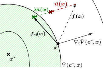
Figure 1: Geometric interpretation of the sequential optimization in Algorithm 1. In red $\hat{\bm{u}}$ shows the control input after only optimizing parameter vector $\bm{c}$, while $\lambda\hat{\bm{u}}$ in green represents the resulting control input after optimizing $\bm{\theta}$. If the conditions in Lemma 4 are met, a sufficiently large $\lambda(\bm{\theta},\cdot)$ s.t. the policy $\bm{\hat{\pi}}(\bm{\theta},\bm{c},\cdot)$ induced by $\hat{V}(\bm{c},\cdot)$ stabilizes the closed-loop system $\bm{f}_{\text{cl}}(\cdot)$ is found.

Intuitively, the first optimization (9bt) finds a candidate $\hat{V}(\bm{c}^{*},\bm{x})$ and the second problem (9bu) scales the resulting control law $\hat{\bm{\pi}}(\bm{\theta}^{*},\bm{c}^{*},\bm{x})$ such that $\hat{V}(\bm{c}^{*},\bm{x})$ is a valid CLF for the system. This is conceptually illustrated in Figure 1. While sequentially solving the SDP problems (9bt) and (9bu) is computationally efficient, the proxy constraint (9bte) leads to a more conservative solutions, as it is a convex inner approximation of the original problem (9bc). However, differently to other shape-constrained polynomial regression concepts [57], the approach in Theorem 2 is less restrictive, since it does not impose strict monotonicity of the gradient of $\hat{V}(\bm{c}^{*},\bm{x})$.

5 Simulation Evaluation

For the evaluation of the proposed approach, we consider two settings. First, we illustrate the inverse optimality of the learned CLF in a scenario where the ground truth value function is known. Here, we show for a nonlinear system that our algorithm is able to recover $V^{*}(\cdot)$ up to a small error.

5.1 Setup and Sample Generation

In order to generate a problem setting where the value function $V^{*}(\cdot)$ is known, we employ the converse HJB (CoHJB) [58]. Given a value function $V^{*}(\cdot)$ and the dynamics component $\bm{g}(\cdot)$, the HJB equation becomes linear in the remaining terms $\bm{f}(\cdot)$, $l(\cdot)$ and $r(\cdot)$. Thus, the CoHJB yields the system dynamics for which a given $V^{*}(\cdot)$ is the value function under the specified cost function. For the polynomial case, the problem reduces to a system of equations in the unknown coefficients of $\bm{f}(\cdot)$. Consider the following nonlinear value function

$$V^{*}=0.1x_{1}^{2}+0.5x_{2}^{2}+x_{1}x_{2}^{2}+x_{1}^{4}+x_{2}^{4},$$ (9bv)

with states $\bm{x}:=[x_{1},x_{2}]^{\intercal}$ and input matrix $\bm{g}(\bm{x})=I_{2}$. Solving the CoHJB problem, we get the open loop system dynamics

$$\bm{f}(x)=\begin{bmatrix}-0.5477x_{1}+0.25x_{2}^{2}+x_{1}^{3}\\ -0.3672x_{2}+0.5x_{1}x_{2}+x_{2}^{3},\end{bmatrix}$$ (9bw)

which are shown in Figure 2 (left). Since $V^{*}(\cdot)$ is known, we can directly compute the optimal policy $\bm{\pi}^{*}(\cdot)$ using (7), thus, providing the closed-loop dynamics $\bm{f}^{*}(\cdot)$, which are illustrated in Figure 2 (right). By introducing state-dependent noise

$$\bm{\sigma}(\bm{x})=\begin{bmatrix}0.001\\ 0.001\end{bmatrix}(x_{1}^{2}+x_{2}^{2}),$$ (9bx)

we further obtain the stochastic closed-loop dynamics (4) from which demonstrations can be sampled. In order to learn the CLF, we observe one-step trajectories of the stochastic closed-loop system dynamics over a grid spanning different parts of the state space. Hence the demonstrations consist of observation tuples $\big{(}\bm{x_{i}},(\bm{f}^{*}(\bm{x_{i}})+\bm{\sigma}(\bm{x_{i}}))\Delta t\big{)}$. Without loss of generality the measurements are normalized, thus, focusing on the state space $\pazocal{X}\in[-1,1]^{2}$. Since the true value function $V^{*}(\cdot)$ is typically unknown, an expressive parameterization for the candidate $\hat{V}(\bm{c},\cdot)$ is chosen, which provides more flexibility during the inference. Here, a degree $d\!=\!8$ is selected, while the true value function is of degree $d^{*}\!=\!4$. Thereby the principle capacity to find $V^{*}(\cdot)$ exists, however, it is required to search over a substantially larger parameter space. As an initial guess we choose $\hat{V}_{0}=0.1\big{(}x_{1}^{2}+x_{2}^{2}\big{)}$ and $\lambda_{0}(x)=0.5$. To solve the SDP problems we employ the YALMIP Matlab toolbox [59] together with the MOSEK SDP solver.

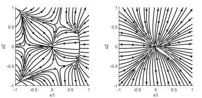
Figure 2: Visualization of the system dynamics. (Left) open-loop dynamics $\bm{f}$ and (right) closed-loop dynamics $\bm{f^{*}}$ under $\bm{\pi}^{*}$.

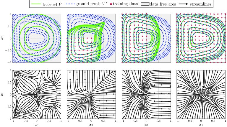
Figure 3: Ground truth evaluation of the proposed algorithm. The top row shows the contours of the ground truth value function $V^{*}(\cdot)$ (blue, dashed) and the learned CLF $\hat{V}(\cdot,\cdot)$ (green). Training data is depicted with purple stars, while the greyed out parts show data free areas. The bottom row illustrates the learned closed-loop dynamics. The learned CLF $\hat{V}(\cdot,\cdot)$ approximates $V^{*}(\cdot)$ well in areas of the state space, where training data is provided. Moreover, the induced closed-loop system is rendered asymptotically stable. Given a dense-enough sampling, the stabilizing policy $\bm{\hat{\pi}}(\cdot,\cdot)$ induces similar dynamics as the optimal policy $\bm{\pi}^{*}(\cdot)$. Note that the first column illustrates the initial guess $\hat{V}_{0}(\cdot,\cdot)$, which only fulfills (9bn) and does not need to constitute a valid CLF.

5.2 Ground Truth Evaluation

Figure 3 shows the obtained results. In the top row of Figure 3, the contours of the ground truth value function $V^{*}(\cdot)$ are shown in blue (dashed) and the contours of the learned CLF $\hat{V}(\cdot,\cdot)$ are shown in green. The grid of observed one-step trajectories is visualized using purple stars, where the star indicates the starting point $\bm{x_{i}}$ of each observation tuple. Conversely, data free areas are illustrated by the greyed out parts of the state space. The bottom row of Figure 3 depicts the resulting closed-loop dynamics induced by the stabilizing control law $\bm{\hat{\pi}}(\cdot,\cdot)$ (9bs) modulated by the gradient of the respective CLF $\hat{V}(\cdot,\cdot)$. From left to right, each column of Figure 3 shows the obtained results for grids spanning a progressively larger area of the state space.

The first column depicts the datafree case with the initial guess $\hat{V}_{0}(\cdot,\cdot)$. As described in Lemma 5, $\hat{V}_{0}(\cdot,\cdot)$ only fulfills condition (9bn) and does not need to constitute a valid CLF. Thus, the related vector field only differ slightly from the open-loop system dynamics and remain unstable.

In the second column a $7\times 7$ grid spanning equidistantly over the lower left quadrant of the normalized state space, i.e., $\bm{x}\in[-1,0]^{2}$, is used to generate training data. Here, it can be seen that the learned $\hat{V}(\cdot,\cdot)$ agrees with the value function $V^{*}(\cdot)$ in the shape of their level curves in areas of the state space, where training data is provided. Moreover, the induced closed-loop dynamics using the stabilizing control law $\bm{\hat{\pi}}(\cdot,\cdot)$ indicate a good reproduction of the dynamics under the optimal policy $\bm{\pi}^{*}(\cdot)$ for the lower left quadrant. On the other hand, in the data free area the learned $\hat{V}(\cdot,\cdot)$ still constitutes a CLF and induces a control policy that globally asymptotically stabilizes the system.

In column three the dataset is extended to a $7\times 14$ grid resulting in 98 samples covering the left half of the normalized state space. With increasing sampling density a better estimate of $V^{*}(\cdot)$ is obtained, resulting in an improved reconstruction of the observed behavior over a larger area.

Finally, column four shows a grid sampling over the complete task space. Our proposed approach yields an estimate $\hat{V}(\cdot,\cdot)$ that matches the ground truth value function $V^{*}(\cdot)$ in the shape of the contour lines up to some small deviations over the whole work space. The system is stabilized under the policy induced by $\hat{V}(\cdot,\cdot)$ and the closed-loop dynamics resemble the ones generated by the optimal policy $\bm{\pi}^{*}(\cdot)$.

Thus, it can be seen that our method is able to retrieve the shape of the true optimal value function $V^{*}(\cdot)$, if provided with sufficient training data. Additionally, the learned CLF $\hat{V}(\cdot,\cdot)$ is directly accompanied by a control law $\hat{\bm{\pi}}(\cdot,\cdot)$, which generates dynamics that closely resembles the demonstration under the optimal policy $\bm{\pi}^{*}(\cdot)$. Intuitively, the CLF $\hat{V}(\cdot,\cdot)$ is optimized to modulate dynamics with an attractor landscape matching the observed demonstrations. Since the control law $\hat{\bm{\pi}}(\cdot,\cdot)$ is asymptotically stabilizing by design, regularity properties are retained by generalizing to unseen areas of the state space by guaranteeing robust convergence to the desired goal state. Moreover, from column two and three in Figure 3 it can be seen that the learned CLF $\hat{V}(\cdot,\cdot)$ does not agree with the value function $V^{*}(\cdot)$ in the data free area, which indicates that the achieved similarity in data rich areas is not artificially enforced due to the parametric structure of $\hat{V}(\cdot,\cdot)$, thus, demonstrating the expressive capabilities of the proposed approach.

6 Learning from Human Demonstrations

While the previous section demonstrates the principle capacity of the learned CLF to approximate an optimal value function, this subsection shows the expressiveness of our method by learning from human demonstrations in a goal-directed movement task. To this end, we perform a benchmark evaluation in which we compare our approach to one state of the art IRL and DMP method using a human handwriting data set [26].

6.1 Comparison Methods

Since our proposed approach conceptually unifies the advantages of IRL and DMP methods, we include one related work of each type here for the performed comparison evaluation. Specifically, we consider adversarial inverse reinforcement learning (AIRL) [20], which is an efficient IRL algorithm applicable in continuous state-action spaces and capable of recovering reward functions that are robust with respect to environment dynamics. Here, both the reward function as well as the policy are parameterized by deep neural networks. Since AIRL is a sampling-based method, it does not require an analytic description of the open-loop dynamics. In contrast to our approach, AIRL infers a reward function, i.e, the stage-costs, which generally contains more information than the value function but does not provide any inherent stability guarantees for the learned policy. Secondly, we compare our approach to a DMP method called CLF-DM (Control Lyapunov Function-based Dynamic Movements) [27], where a task-oriented, CLF-like function is learned from data to generate stable dynamical systems using a virtual, stabilizing controller. The process of learning the CLF, the dynamics and the virtual controller is split into three distinct steps, thereby the motion encoding and stabilization are separated, which is in contrast to our integrated approach. Moreover, [27] is a DMP method, and thus, only generates motion plans and not an actual control policy that can be applied to a real system.

6.2 Demonstration Data and Evaluation Setup

We evaluate all methods on the real-world LASA handwriting data set [26], which consists of 30 human-drawn trajectories of various letters and shapes with 7 demonstrations each. The data set is commonly used to compare approaches for learning from demonstration. All data is normalized to a state space $\pazocal{X}\in[-1,1]^{2}$. While the LASA data set itself does not provide information regarding the dynamics, we consider unstable, polynomial systems of degree 3 for the open-loop environment dynamics of each shape. Thereby, it is emulated that the provided demonstrations represent an agent acting on a dynamical system and allows for a non-trivial modelling of the agent by means of the inferred value function. The resulting open-loop dynamics and the demonstration data are illustrated for 4 exemplary shapes in Figure 4.

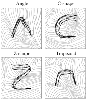
Figure 4: Depiction of 4 exemplary shapes of the LASA handwriting dataset. The associated, unstable open-loop dynamics (gray) are polynomial functions of degree 3. The demonstrations shown with black dots are generated by an agent acting on the dynamical system.

For the training $N=7$ demonstrations are observed per shape, where each demonstration trajectory includes $T=1000$ samples resulting in a total data set size of $7000$ per shape. Due to the stochastic initialization strategies of the AIRL algorithm, training is performed for 5 different seeds with $1000$ iterations each, from which the seed with the best tracking performance is selected for the comparison evaluation. The network size is chosen to 3 hidden layers, each consisting of $64$ neurons for both the reward and the policy network. For CLF-DM we use the proposed Weighted Sum of Asymmetric Quadratic Function (WSAQF) with $\mathscr{L}=3$ asymmetric functions to learn the energy function. Furthermore, a Gaussian Mixture Regression consisting of 8 components is used to fit the dynamical system. Finally, for our proposed approach, a degree of $\text{deg}(\hat{V})=8$ is chosed for $\hat{V}(\bm{c},\cdot)$ and $\text{deg}(\lambda)=16$ for $\lambda(\bm{\theta},\cdot)$. Algorithm 1 is initialized with $\hat{V}_{0}(\bm{x})=x_{1}^{2}+x_{2}^{2}$ and $\bm{\lambda}_{0}(\bm{x})=0.5\bm{I}_{2}$ and configured to run for 5 iterations. Moreover, the regularization factor is set to of ${\bm{\Sigma}_{c}^{-1}=10^{-4}\bm{I}_{2}}$. The reproduction performance is evaluated using three similarity measures, i.e., mean squared error (MSE), piecewise curve mapping (PCM) and dynamic time warping (DTW), for which the implementation in [60] is used.

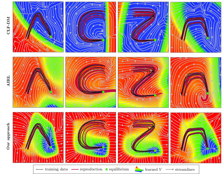
Figure 5: Comparison of the learned $\hat{V}(\cdot,\cdot)$ and reproductions for the our proposed approach, AIRL and CLF-DM. The reproductions are illustrated by a red line and the training data is represented by black dots. The learned potential functions are visualized in the form of a projected surface plot underlying the streamlines (gray arrows). Here, the shape encoding in the learned CLF is clearly visible for our approach, as the potential function shrinks along the vector field and the minimum coincides with the target state. Moreover, our method demonstrates convergence to the equilibrium for all shapes.

6.3 Benchmark Evaluation

The results of the comparison evaluation are depicted for the 4 exemplary shapes in Figure 5. Here, both the learned value function, in the case of AIRL, and learned Lyapunov function for CLF-DM and our approach are visualized together with the resulting vector field. Note that the vector fields for our method and AIRL indicate the closed-loop dynamics under the associated policy, while the ones shown for CLF-DM merely represent the learned, virtual dynamics and not a controlled, closed-loop system.

Reproduction performance

When inspecting the reproduced trajectories, it can be seen directly that our method and CLF-DM induce asymptotic convergence to the desired equilibrium for all shapes. In contrast, AIRL produces unstable closed-loop dynamics for the C-shape and convergence to a spurious attractor in the case of the Z-shape and Trapezoid. As there are no guarantees for the learned policy, this behavior varies for each scenario. Hence, even in cases where the reproductions converge to the desired equilibrium, no statement regarding the region of attraction or generalization properties can be made. When inspecting the reproductions it can be seen that CLF-DM and our approach generate more dynamic motion, while AIRL generally induces smoother trajectories. However, in particular for highly dynamic demonstrations, our method exhibits a skipping behavior in some instances, where a conservative convergence to the equilibrium is induced.

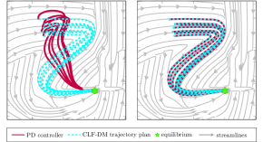
Figure 6: Comparison of two control parametrization, i.e., (left) a low-gain and (right) a high-gain PD controller, to track the trajectory plan generated by CLF-DM for the Z-shape. It can be seen that the reproduction performance is highly dependent on the design choice of the tracking controller.

Quantitative evaluation

In order to perform a more rigorous comparison, a quantitative evaluation is provided in Section 6.3. Here, we compare the reproduction similarity for the respective shapes depicted in Figure 5 together with the average over all 30 shapes included in the dataset. It can be seen that AIRL exhibits a better performance according to the MSE. However, for similarity measures that are strongly related to the geometric accuracy of curves (PCM and DTW), our method consistently outperforms AIRL. Moreover, due to a lack of convergence guarantees, the reproduction quality of AIRL suffers greatly if task success is explicitly linked to reaching a specific goal state exactly, which cannot be expressed by the similarity measures depicted in Section 6.3. Therefore, our approach generates superior reproductions in terms of geometric similarity to the observed demonstrations and guaranteed convergence to the desired target state. Note that the measures achieved by CLF-DM are grayed out in Section 6.3, since it merely represents a trajectory plan and the achieved reproduction primarily depends on the design of a subsequent tracking controller. This can be seen in Figure 6 which illustratively depicts the achieved tracking performance when deploying a PD controller $\bm{u}_{\text{PD}}(\bm{x},\dot{\bm{x}})\coloneqq\bm{K}_{P}(\bm{x}_{\text{ref}}-\bm{x})+\bm{K}_{D}(\bm{\dot{x}}_{\text{ref}}-\bm{\dot{x}})$ to track the trajectory plan $\{\bm{x}_{\text{ref}},\bm{\dot{x}}_{\text{ref}}\}$ generated by CLF-DM for two different control gain parametrization, i.e., a low-gain parametrization $\bm{K}_{P,\text{low}}=0.5\bm{I}_{2}$, $\bm{K}_{D,\text{low}}=0.05\bm{I}_{2}$ and a high-gain parametrization $\bm{K}_{P,\text{high}}=50\bm{I}_{2}$, $\bm{K}_{D,\text{high}}=1.0\bm{I}_{2}$. It is clearly visible that the achieved reproductions primarily depend on the design of the tracking controller which is not trivial in general. Thus, a direct comparison of the output provided by CLF-DM and the one generated by our approach and AIRL with respect to reproductions is difficult.

mystyle late after line= ,

Intention encoding

Besides obtaining a policy that replicates the observed demonstrations, one of the key benefits of IRL methods is the inference of a cost function representation, which facilitates interpretability by modelling the underlying agent intention. In Figure 5 the associated potential functions, e.g., value function, task-oriented CLF or CLF-based value function approximation, represent this intention. For the CLF-DM method the shapes are not attributable to the task-oriented CLF, even though it is learned from the demonstrations. Since the process of learning the CLF, the dynamic system and the virtual, stabilizing controller is separated, the coherence of the retained CLF to a given reproduction result is not guaranteed. On the other hand, despite the cost function inference performed by AIRL, the resulting value functions depicted in Figure 5 is not unambiguously relatable to the demonstrated shapes. This is since nonlinear IRL methods, such as [18, 19, 20], only approximately solve the computationally demanding forward optimal control problem that iteratively occurs during the cost function inference. In the case of AIRL for instance, only a few RL iterations are performed to learn the optimal policy for the current reward function parametrization instead of running the algorithm to convergence, thereby accelerating the inference process. However, while the pair of retrieved cost function and policy reproduce the demonstrations well, the two functions are no longer consistently related due to the performed approximation. Hence, the inferred cost function may not represent the underlying intention anymore. In contrast, for our approach the demonstrated shapes are clearly visible in the projected surface plots of the learned CLF-based value function approximation. This is since our method completely encodes the generated motion through the Lyapunov function, as the closed-form stabilizing policy $\bm{\hat{\pi}}(\cdot,\cdot)$ is directly dependent on the gradient of the CLF. By exploiting this analytical link it is possible to directly search over the space of parametrization of $\hat{V}(\cdot,\cdot)$ by optimizing the attractor landscape of the generated closed-loop dynamical system to capture the observed demonstration. Thereby we achieve an efficient and fully integrated learning process, where the inferred CLF induces a control vector field that reproduces the demonstrations, while also guaranteeing asymptotic convergence to the task goal by design. Moreover, through the closed-form expressions we obtain consistently interpretable solutions.

Table 1: Resulting mean squared error (MSE), dynamic time warping (DTW) and piecewise curve mapping (PCM) measures over 4 shapes and the average over all shapes. For each measure, the mean along with the standard deviation calculated from all 7 reproductions per shape is given.

	MSE $\times 10^{3}$			DTW			PCM
	Our	AIRL	CLF-DM	Our	AIRL	CLF-DM	Our	AIRL	CLF-DM
[mystyle]evaluation_data/measures_unextended.csv	$67{\pm}33$	$\textbf{8}{\pm}\textbf{5}$	$13{\pm}12$	$124{\pm}66.4$	$333{\pm}33.9$	${\color[rgb]{.5,.5,.5}\textbf{70}{\pm}\textbf{31.5}}$	$85.5{\pm}35.5$	$334.3{\pm}41.5$	${\color[rgb]{.5,.5,.5}\textbf{54.5}{\pm}\textbf{30.5}}$

7 Conclusion

In this article, we propose a novel approach for performing stable IRL by exploiting the inverse optimal relation between the value function and control Lyapunov functions. In particular, we reformulate the cost function inference to learning a Lyapunov-constrained value function approximation. For the continuous evaluation of the value function, we propose the use of gradient-based, stabilizing control laws leading to a closed-form expression of the log-likelihood. Due to the analytic expressions, the optimization of $\hat{V}(\cdot,\cdot)$ is intuitively analogue to a search over the space of point-attractor landscapes spanned by the closed-loop dynamics. We perform a theoretical analysis for the CLF-based approximation and demonstrate under which conditions optimality properties are retained. Additionally, we present how inverse optimal CLFs are efficiently learned from data using the SOS technique. First, an equivalent, convex reformulation of the posterior expressions is derived. Second, the Lyapunov-constrained problem is convexified by proposing a sequential, two-step optimization approach. The algorithm allows for the efficient inference of CLFs $\hat{V}(\cdot,\cdot)$ and guarantees that the closed-loop dynamics under policy $\hat{\bm{\pi}}(\cdot,\cdot)$ are asymptotically stable. In the evaluation, we show that our proposed framework exhibits the desired convergence properties and performs superior in encoding the preferences of a human demonstrator in comparison to a state-of-the-art IRL and DMP method.

References

- [1] A. Mohebbi, “Human-Robot Interaction in Rehabilitation and Assistance: a Review,” Current Robotics Reports, vol. 1, pp. 131–144, 2020.
- [2] S. E. Hashemi-Petroodi, S. Thevenin, S. Kovalev, and A. Dolgui, “Operations management issues in design and control of hybrid human-robot collaborative manufacturing systems: a survey,” pp. 264–276, 2020.
- [3] C. You, J. Lu, D. Filev, and P. Tsiotras, “Advanced planning for autonomous vehicles using reinforcement learning and deep inverse reinforcement learning,” Robotics and Autonomous Systems, vol. 114, pp. 1–18, 2019.
- [4] A. Hussein, M. M. Gaber, E. Elyan, and C. Jayne, “Imitation learning: A survey of learning methods,” ACM Computing Surveys, vol. 50, 2017.
- [5] H. Ravichandar, A. S. Polydoros, S. Chernova, and A. Billard, “Recent Advances in Robot Learning from Demonstration,” Annual Review of Control, Robotics, and Autonomous Systems, vol. 3, pp. 297–330, 2020.
- [6] S. Raza, S. Haider, and M. A. Williams, “Teaching coordinated strategies to soccer robots via imitation,” in Proceedings of the IEEE International Conference on Robotics and Biomimetics, 2012, pp. 1434–1439.
- [7] S. Arora and P. Doshi, “A survey of inverse reinforcement learning: Challenges, methods and progress,” Artificial Intelligence, vol. 297, p. 103500, 2021.
- [8] P. Abbeel and A. Y. Ng, “Apprenticeship learning via inverse reinforcement learning,” in Proceedings of the International Conference on Machine Learning, 2004, pp. 1–8.
- [9] W. L. Nelson, “Physical principles for economies of skilled movements,” Biological Cybernetics, vol. 46, pp. 135–147, 1983.
- [10] T. Flash and N. Hogan, “The coordination of arm movements: An experimentally confirmed mathematical model,” Journal of Neuroscience, vol. 5, pp. 1688–1703, 1985.
- [11] E. Todorov, “Optimality principles in sensorimotor control,” Nature Neuroscience, vol. 7, pp. 907–915, 2004.
- [12] S. Russell, “Learning agents for uncertain environments,” in Proceedings of the annual conference on Computational learning theory, 1998, pp. 101–103.
- [13] A. Ng and S. Russell, “Algorithms for inverse reinforcement learning,” in Proceedings of the International Conference on Machine Learning, 2000, pp. 663–670.
- [14] N. D. Ratliff, J. Andrew Bagnell, and M. A. Zinkevic, “Maximum margin planning,” in Proceedings of the International Conference on Machine Learning, vol. 148, 2006, pp. 729–736.
- [15] B. D. Ziebart, A. Maas, J. A. Bagnell, and A. K. Dey, “Maximum entropy inverse reinforcement learning,” in Proceedings of the National Conference on Artificial Intelligence, vol. 3, 2008, pp. 1433–1438.
- [16] B. D. Ziebart, J. A. Bagnell, and A. K. Dey, “Modeling Interaction via the Principle of Maximum Causal Entropy,” in Proceedings of the International Conference on Machine Learning, 2010, pp. 1255–1262.
- [17] N. Aghasadeghi and T. Bretl, “Maximum entropy inverse reinforcement learning in continuous state spaces with path integrals,” in IEEE/RSJ International Conference on Intelligent Robots and Systems, 2011, pp. 1561–1566.
- [18] C. Finn, S. Levine, and P. Abbeel, “Guided cost learning: Deep inverse optimal control via policy optimization,” in Proceedings of the International Conference on Machine Learning, vol. 1, 2016, pp. 95–107.
- [19] C. Finn, P. Christiano, P. Abbeel, and S. Levine, “A Connection between Generative Adversarial Networks, Inverse Reinforcement Learning, and Energy-Based Models,” in NIPS Workshop on Adversarial Training, 2016.
- [20] J. Fu, K. Luo, and S. Levine, “Learning robust rewards with adversarial inverse reinforcement learning,” in Proceedings of the International Conference on Learning Representations (ICLR), 2018.
- [21] M. C. Priess, R. Conway, J. Choi, J. M. Popovich, and C. Radcliffe, “Solutions to the inverse lqr problem with application to biological systems analysis,” IEEE Transactions on Control Systems Technology, vol. 23, pp. 770–777, 2015.
- [22] F. Ornelas-Tellez, E. N. Sanchez, and A. G. Loukianov, “Discrete-time neural inverse optimal control for nonlinear systems via passivation,” IEEE Transactions on Neural Networks and Learning Systems, vol. 23, pp. 1327–1339, 2012.
- [23] A. Jan Ijspeert, J. Nakanishi, and S. Schaal, “Learning Attractor Landscapes for Learning Motor Primitives,” in Proceedings of the International Conference on Neural Information Processing Systems, vol. 15, 2002.
- [24] S. Schaal, A. Ijspeert, and A. Billard, “Computational approaches to motor learning by imitation,” Philosophical Transactions of the Royal Society B: Biological Sciences, vol. 358, pp. 537–547, 2003.
- [25] P. Pastor, H. Hoffmann, T. Asfour, and S. Schaal, “Learning and generalization of motor skills by learning from demonstration,” in Proceedings of the IEEE International Conference on Robotics and Automation, 2009, pp. 763–768.
- [26] S. M. Khansari-Zadeh and A. Billard, “Learning stable nonlinear dynamical systems with Gaussian mixture models,” IEEE Transactions on Robotics, vol. 27, pp. 943–957, 2011.
- [27] ——, “Learning control Lyapunov function to ensure stability of dynamical system-based robot reaching motions,” Robotics and Autonomous Systems, vol. 62, pp. 752–765, 2014.
- [28] J. Umlauft and S. Hirche, “Learning stochastically stable Gaussian process state–space models,” IFAC Journal of Systems and Control, vol. 12, p. 100079, 2020.
- [29] R. E. Kalman, “When is a linear control system optimal?” Journal of Basic Engineering, vol. 86, pp. 51–60, 1964.
- [30] R. A. Freeman and P. V. Kokotovic, “Inverse optimality in robust stabilization,” SIAM Journal on Control and Optimization, vol. 34, pp. 1365–1391, 1996.
- [31] M. Krstić and Z. H. Li, “Inverse optimal design of input-to-state stabilizing nonlinear controllers,” IEEE Transactions on Automatic Control, vol. 43, pp. 336–350, 1998.
- [32] S. Tesfazgi, A. Lederer, and S. Hirche, “Inverse Reinforcement Learning: A Control Lyapunov Approach,” in Proceedings of the IEEE Conference on Decision and Control, 2021, pp. 3627–3632.
- [33] J. Schoukens and L. Ljung, “Nonlinear System Identification: A User-Oriented Road Map,” IEEE Control Systems, vol. 39, pp. 28–99, 2019.
- [34] N. Hogan, “Impedance control: An approach to manipulation,” in Proceedings of the American Control Conference, vol. 1, 1984, pp. 304–313.
- [35] D. A. Winter, Biomechanics and Motor Control of Human Movement. Wiley, sep 2009.
- [36] C. J. Hasson, O. Gelina, and G. Woo, “Neural control adaptation to motor noise manipulation,” Frontiers in Human Neuroscience, vol. 10, 2016.
- [37] S. Schaal, “Is imitation learning the route to humanoid robots?” Trends in Cognitive Sciences, vol. 3, pp. 233–242, 1999.
- [38] H. K. Khalil, Khalil, Nonlinear Systems, 3rd Edition. Upper Saddle River: NJ: Prentice-Hall, 2002.
- [39] W. H. Fleming and H. Soner, Controlled Markov Processes and Viscosity Solutions. New York: Springer-Verlag, 2006.
- [40] J. A. Primbs, V. Nevistić, and J. C. Doyle, “Nonlinear optimal control: A control Lyapunov function and receding horizon perspective,” Asian Journal of Control, vol. 1, pp. 14–24, 2008.
- [41] R. Khasminskii, Stochastic Stability of Differential Equations (Stochastic Modelling and Applied Probability). Springer, 2011.
- [42] A. A. Ahmadi and P. A. Parrilo, “Converse results on existence of sum of squares Lyapunov functions,” in Proceedings of the IEEE Conference on Decision and Control, 2011, pp. 6516–6521.
- [43] T. Rajpurohit and W. M. Haddad, “Lyapunov and converse Lyapunov theorems for stochastic semistability,” Systems and Control Letters, vol. 97, pp. 83–90, nov 2016.
- [44] Z. Artstein, “Stabilization with relaxed controls,” Nonlinear Analysis, vol. 7, pp. 1163–1173, 1983.
- [45] E. D. Sontag, “A ’universal’ construction of Artstein’s theorem on nonlinear stabilization,” Systems and Control Letters, vol. 13, pp. 117–123, 1989.
- [46] R. Freeman and J. Primbs, “Control lyapunov functions: new ideas from an old source,” in Proceedings of the IEEE Conference on Decision and Control, vol. 4, 1996, pp. 3926–3931.
- [47] P. A. Parrilo, “Structured semidefinite programs and semialgebraic geometry methods in robustness and optimization,” Ph.D. dissertation, California Institute of Technology, Pasadena, CA, 2000.
- [48] A. A. Ahmadi and B. E. Khadir, “Learning Dynamical Systems with Side Information,” in Proceedings of the Conference on Learning for Dynamics and Control, vol. 120, 2020, pp. 718–727.
- [49] S. Boyd and L. Vandenberghe, Convex Optimization, 1st ed. Cambridge: Cambridge University Press, 2004.
- [50] F. Zhang, The Schur Complement and its Applications, ser. Numerical Methods and Algorithms. New York: Springer, 2005, vol. 4.
- [51] A. Papachristodoulou and S. Prajna, “A tutorial on sum of squares techniques for systems analysis,” in Proceedings of the American Control Conference, vol. 4, 2005, pp. 2686–2700.
- [52] Y. Wang and R. Rajamani, “Feasibility analysis of the bilinear matrix inequalities with an application to multi-objective nonlinear observer design,” in Proceedings of the IEEE Conference on Decision and Control, 2016, pp. 3252–3257.
- [53] K.-C. Goh, M. G. Safonov, and G. P. Papavassilopoulos, “Global optimization for the Biaffine Matrix Inequality problem,” Journal of Global Optimization, vol. 7, pp. 365–380, 1995.
- [54] J. B. Lasserre, “Global Optimization with Polynomials and the Problem of Moments,” SIAM Journal on Optimization, vol. 11, pp. 796–817, 2001.
- [55] Q. Tran Dinh, W. Michiels, S. Gros, and M. Diehl, “An inner convex approximation algorithm for BMI optimization and applications in control,” in Proceedings of the IEEE Conference on Decision and Control, dec 2012, pp. 3576–3581.
- [56] K. C. Goh, L. Turan, M. G. Safonov, G. P. Papavassilopoulos, and J. H. Ly, “Biaffine matrix inequality properties and computational methods,” in Proceedings of the American Control Conference, 1994, pp. 850–855.
- [57] M. Curmei and G. Hall, “Shape-Constrained Regression using Sum of Squares Polynomials,” Operations Research, 2023.
- [58] J. Doyle, J. A. Primbs, B. Shapiro, and V. Nevistic, “Nonlinear games: Examples and counterexamples,” in Proceedings of the IEEE Conference on Decision and Control, vol. 4, 1996, pp. 3915–3920.
- [59] J. Löfberg, “YALMIP: A toolbox for modeling and optimization in MATLAB,” in Proceedings of the IEEE International Symposium on Computer-Aided Control System Design, 2004, pp. 284–289.
- [60] C. F. Jekel, G. Venter, M. P. Venter, N. Stander, and R. T. Haftka, “Similarity measures for identifying material parameters from hysteresis loops using inverse analysis,” International Journal of Material Forming, vol. 12, pp. 355–378, 2019.