Robust self-testing of Bell inequalities tilted for maximal loophole-free nonlocality

Abstract

The degree of experimentally attainable nonlocality, as gauged by the amount of loophole-free violation of Bell inequalities, remains severely limited due to inefficient detectors. We address an experimentally motivated question: Which quantum strategies attain the maximal loophole-free nonlocality in the presence of inefficient detectors? For any Bell inequality and any specification of detection efficiencies, the optimal strategies are those that maximally violate a tilted version of the Bell inequality in ideal conditions. In the simplest scenario, we demonstrate that the quantum strategies that maximally violate the tilted versions of Clauser-Horne-Shimony-Holt inequality are unique up to local isometries. However, self-testing via the standard sum of squares decomposition method turns out to be analytically intractable since even high levels of the Navascués–Pironio–Acín hierarchy are insufficient to saturate the maximum quantum violation of these inequalities. Instead, we utilize a novel Jordan’s lemma-based proof technique to obtain robust analytical self-testing statements for the entire family of tilted-Bell inequalities. These results allow us to unveil intriguing aspects of the effect of inefficient detectors and the complexity of characterizing the set of quantum correlations, in the simplest Bell scenario.

I Introduction

Correlations born of local measurements performed on entangled quantum systems shared between distant observers resist local-causal explanations, a phenomenon known as Bell nonlocality [1, 2]. Apart from their foundational significance, nonlocal correlations enable several classically impossible information processing and cryptographic feats such as unconditionally secure Device-Independent Quantum Key Distribution (DIQKD) [3, 4, 5, 6, 7]. The efficacy of these applications relies on loophole-free certification of strong nonlocal correlations. In particular the detection loophole, which results of performing a Bell test with inefficient detectors, is the most persistent obstacle in the experimental realization of strong long-range loophole-free nonlocal correlations.

The detection efficiency of a measuring party is the ratio of particles detected to the total number of particles emitted by the source. The effective detection efficiency $\eta$ depends on the detectors and the device’s distance from the source. For instance, in photonic Bell experiments, the effective detection efficiency decays exponentially with the length of the optical fiber, $l$, such that $\eta=\eta_{0}10^{-\frac{\alpha l}{10}}$, where $\eta_{0}$ is the detection efficiency of the measuring apparatus due to the use of imperfect detectors, and $\alpha$ is the attenuation coefficient [8]. Closing the detection loophole in Bell experiments amounts to having an effective detection efficiency $\eta$ higher than a threshold value $\eta^{*}$, referred to as the critical detection efficiency. Typically, $\eta^{*}$ is a characteristic of an ideal nonlocal correlation, below which it ceases to be nonlocal, and limits the distance across which nonlocality can be operationally certified to $l<\frac{10}{\alpha}\log(\frac{\eta^{*}}{\eta_{0}})$.

In the simplest bipartite Bell scenario, the quantum strategy maximally violating the Clauser-Horne-Shimony-Holt (CHSH) inequality (in ideal conditions) ceases to yield nonlocal correlations for detector efficiencies below $\eta^{*}=2\sqrt{2}-2\simeq 0.82$ [9]. However, for an almost product entangled state, this threshold efficiency can be lowered to $2/3\simeq 0.66$ [10], which comes at the cost of very low robustness to background noise. Significant research efforts have been directed towards minimizing the critical detection efficiency requirement for loophole-free certification of nonlocality [11, 12, 13, 14]. However, for real-world applications to be effective, mere violation of a Bell inequality is insufficient [15]. Instead, the efficacy of such applications [14] typically requires high degree of nonlocality and motivates the question:

Which quantum strategies yield the maximum loophole-free nonlocality in the presence of inefficient detectors?

As the extent of the violation of a (facet) Bell inequality corresponds to the distance of a nonlocal correlation from a facet of the local polytope, it translates to a reliable measure of nonlocality. Thus the question above boils down to finding the quantum strategies that yield the maximal loophole-free violation of a given Bell inequality for specified detection efficiencies. Since the use of inefficient detectors results in the occurrence of ”no-click” events, to decide whether a given inequality is violated these events must be included in the measurement statistics. The most general way to deal with them is to treat them as an additional outcome, which comes at the price of enlarging the Bell scenario. However, to analyse the violation of a given Bell inequality, we need to consider post-processing strategies which do not alter the Bell scenario. One such experimentally convenient post-processing, which avoids considering additional outcomes as well as the fair-sampling assumption, is to assign a valid outcome to the “no-click” event [16]. Moreover, such local assignment strategies were proven to be optimal in the CHSH scenario [17].

We use the assignment strategies described above to show that the quantum state and measurements maximally violating a given Bell inequality, in the presence of inefficient detectors, correspond to those maximally violating, in ideal conditions, a tilted version of the inequality. In the simplest Bell scenario, where up to a relabeling of measurements and outcomes the only facet inequality is the CHSH inequality, attaining maximal loophole-free nonlocality amounts to maximally violating a doubly-tilted version of CHSH. Such inequalities can be thought of as a generalization of the ones considered in Ref. [18, 19], which correspond to the case of one party having access to ideal detectors, and for which both the maximal violation and the quantum realization attaining it are known. In fact, in Ref. [18] it is shown by means of sum-of-squares (SOS) decompositions that the optimal state and measurements are unique up to local unitaries, i.e., the maximal violation self-tests the optimal quantum strategy.

These self-testing results suggest that analogous results could be derived for the general doubly-tilted CHSH inequalities. However, for this general case self-testing via the standard SOS decomposition methods used in [18] turns out to be analytically intractable. On one hand, unlike the case of one imperfect detector, both the maximal quantum violation and the realization attaining it have a more intricate dependence on the detection efficiencies. This complexity translates to the coefficients of the polynomials in a tight SOS decomposition. On the other hand, most strikingly, for the general case, even higher levels (up to level 10) of the Navascués–Pironio–Acín (NPA) hierarchy are not enough to saturate the maximal violation of the doubly-tilted CHSH inequalities. This result highlights the complexity of characterizing the quantum set of correlations even in the simplest Bell scenario. In particular, as the degree of the polynomials in a tight SOS decomposition corresponds to the level of a tight NPA upper bound, finding such polynomials becomes a hard task.

Instead, we derive analytical self-testing statements and optimal quantum strategies for the entire family of doubly-tilted CHSH inequalities as a function of detection efficiencies, via a novel proof technique based on Gröbner basis reduction and Jordan’s lemma (Chapter VII [20]). We find that the optimal quantum strategy entails a partially entangled two-qubit state and non-maximally incompatible observables for both parties. In particular, in contrast to the case of one imperfect detector, in general, the optimal observables of a party also depend on the detection efficiency of the other party. The analytical results allow us to reveal intriguing aspects of the set of quantum correlations in the simplest Bell scenario. Finally, we numerically demonstrate the robustness of these self-testing statements. We conclude by enlisting several implications of our findings to device independent processing with inefficient detectors and to the complexity of characterization of the set of quantum correlations.

II Nonlocality with imperfect detectors

In this section we discuss how nonlocal correlations can be detected via violation of a Bell inequality in presence of non-ideal detectors. Building on these observations, we show that maximising the effective violation of a Bell inequality in the presence of imperfect detectors amounts to maximally violating a tilted version of the inequality in ideal conditions.

Consider a bipartite Bell experiment involving two parties, Alice and Bob. In each round of such experiment a source distributes a composite physical system to be shared between Alice and Bob. Alice performs one out of $m_{A}$ possible measurements that we label with $x$, each of which has $d_{A}$ possible outcomes labeled by $a$. Bob performs one out of $m_{B}$ possible measurements, labeled by $y$, which results in one out of $d_{B}$ outcomes, labeled by $b$. Together, the tuple $(m_{A},m_{B},d_{A},d_{B})$ uniquely specifies a bipartite Bell scenario. In what follows we will denote by $p(ab|xy)$ the probability of Alice and Bob obtaining outcomes $a$ and $b$ conditioned on performing measurements $x$ and $y$, respectively. We also denote by $\bm{p}\in\mathbb{R}^{m_{A}d_{A}m_{B}d_{B}}$, the vectors with entries $p(ab|xy)$, commonly referred to as a behavior.

Let us now recall that for any Bell scenario, the set $\mathcal{L}$ of behaviors admitting local-causal explanations forms a convex polytope. The vertices of $\mathcal{L}$ are local deterministic behaviors [21], for which $p(ab|xy)=p_{A}(a|x)p_{B}(b|y)$, with marginals $p_{A}(a|x),p_{B}(b|y)\in\{0,1\}$. While any behavior $\bm{p}$ in $\mathcal{L}$ admits a quantum realization, i.e., there exists quantum strategies entailing a bipartite quantum state $\hat{\rho}_{AB}$ and local quantum measurement operators $\{\hat{M}_{a}^{x},\hat{N}_{b}^{y}\}$ such that,

$$p(ab|xy)=\Tr\;\left(\hat{\rho}_{AB}\,\hat{M}_{a}^{x}\otimes\hat{N}_{b}^{y}\right)\qquad\forall\;a,b,x,y\;,$$ (1)

the converse does not hold. Specifically, there are behaviors admitting a quantum realization that cannot be expressed as a convex combination of local deterministic behaviors. Therefore, the set $\mathcal{Q}$ of quantum behaviors strictly contains the local set, $\mathcal{L}\subset\mathcal{Q}$. We say that a quantum behavior $\bm{p}$ is nonlocal if $\bm{p}\in\mathcal{Q}\setminus\mathcal{L}$.

Each facet of $\mathcal{L}$ is associated with an inequality of the form

$$\beta(\bm{p}):=\sum_{a,b,x,y}c^{xy}_{ab}p(ab|xy)\leq\beta_{\mathcal{L}},$$ (2)

with $c^{xy}_{ab},\beta_{\mathcal{L}}\in\mathbb{R}$, which is satisfied by all local behaviors.

It follows then that a nonlocal behavior $\bm{p}$ must violate at least one of these facet Bell inequalities, with the amount of the violation, $\beta(\bm{p})-\beta_{\mathcal{L}}$, related to the distance of $\bm{p}$ to the corresponding facet, which can be thought of as a measure on nonlocality [22].

Note that, up to this point, the experimental setups have been assumed to be ideal. In particular, the detectors are perfect as they always detect an incoming quantum system. In actual experiments, however, detectors are not perfect and will sometimes fail to click, which results in the occurrence of ”no-click” events that so far were not considered in the measurement statistics. We describe in the following the effect of imperfect detectors on nonlocal quantum behaviors in Bell experiments, and in particular, on the violation of Bell inequalities.

The most general way of accounting for a “no-click” event is to consider it an additional outcome, say $\Phi$, of the measurement, which enlarges the Bell scenario to $(m_{A},m_{B},d_{A}+1,d_{B}+1)$, significantly increasing the complexity of characterizing the sets $\mathcal{L},\mathcal{Q}$. We can avoid this problem and the fair-sampling assumption, while remaining in the same scenario, by using a more convenient post-processing which assigns a pre-existing outcome to each “no-click” event. Besides the experimental benefits of a smaller Bell scenario, this method is well-suited for our purposes, since we are interested in gauging the effect of imperfect detectors on the value of a given Bell inequality and retrieving the optimal quantum strategies.

Let us suppose that Alice’s and Bob’s measurement devices click with efficiencies $\eta_{A},\eta_{B}<1$, respectively. Whenever Alice’s device fails to click she assigns a pre-existing outcome $a$ with probability $q_{A}(a|x)$. Similarly, Bob assigns $b$ with probability $q_{B}(b|y)$ whenever his device fails to click. Together, the vector of probabilities $q(ab|xy)=q_{A}(a|x)q_{B}(b|y)$ specify a local assignment strategy $\bm{q}$. Let $p(ab|xy)$ be the ideal joint probabilities, then the effective measurement statistics $\tilde{p}(ab|xy)$ are determined by,

$$\tilde{p}(ab|xy)= \eta_{A}\eta_{B}p(ab|xy)+\eta_{A}(1-\eta_{B})p_{A}(a|x)q_{B}(b|y)$$

$$+(1-\eta_{A})\eta_{B}q_{A}(a|x)p_{B}(b|y)$$

$$+(1-\eta_{A})(1-\eta_{B})q_{A}(a|x)q_{B}(b|y).$$ (3)

Hence, for any local assignment strategy $\bm{q}$, the effect of inefficient detectors is a linear map $\tilde{\bm{p}}=\Omega_{\eta_{A}\eta_{B}}(\bm{p})$ such that,

$$\tilde{\bm{p}}=\Omega_{\eta_{A}\eta_{B}}(\bm{p})= \eta_{A}\eta_{B}{\bm{p}}+\eta_{A}(1-\eta_{B}){\bm{p}}^{A}$$

$$+(1-\eta_{A})\eta_{B}{\bm{p}}^{B}+(1-\eta_{A})(1-\eta_{B})\bm{q},$$ (4)

where the effective behavior $\tilde{\bm{p}}$ has entries $\tilde{p}(ab|xy)$, and the vectors ${\bm{p}}^{A},{\bm{p}}^{B}$ linearly depend on the ideal marginal probabilities $p_{A}(a|x),p_{B}(b|y)$, and have entries ${p}_{A}(a|x)q_{B}(b|y)$, $q_{A}(a|x){p}_{B}(b|y)$, respectively, for any $\eta_{A},\eta_{B}$ and $\bm{q}$. Consequently, by linearity, the value of a given Bell functional $\beta$ over this effective behavior takes the form,

$$\beta(\tilde{\bm{p}})= \eta_{A}\eta_{B}\beta(\bm{p})+\eta_{A}(1-\eta_{B})\beta({\bm{p}}^{A})+(1-\eta_{A})\eta_{B}\beta({\bm{p}}^{B})$$

$$+(1-\eta_{A})(1-\eta_{B})\beta(\bm{q}).$$ (5)

Since locally assigning a pre-existing outcome to the “no-click” is essentially a local post-processing, it cannot increase the local bound of a Bell inequality $\beta(\bm{p})\leq\beta_{\mathcal{L}}$ (2). Hence, a Bell experiment with inefficient detectors is said to possess loophole-free nonlocality, if the effective behavior $\tilde{\bm{p}}$ violates the same Bell inequality, i.e.,

$$\beta(\tilde{\bm{p}})\leq\beta_{\mathcal{L}}.$$ (6)

Consequently, we naturally arrive at the question of determining the maximum achievable loophole-free violation, $\beta(\tilde{\bm{p}})-\beta_{\mathcal{L}}$, for a given Bell inequality. Note that the optimization problem involved in the computation of this maximal violation is twofold, since we need two optimize over both local assignments and quantum strategies. In the next Lemma, we greatly simplify this problem by showing that the optimal assignment strategy is necessarily deterministic, which results in a family of tilted Bell inequalities whose maximal violation in ideal circumstances corresponds to the maximum loophole-free violation of the Bell inequality in presence of inefficient detectors.

Lemma 1.

Consider a Bell experiment with inefficient detection with efficiencies $\eta_{A},\eta_{B}$. For any given Bell inequality $\beta({\bm{p}})\leq\beta_{\mathcal{L}}$ (2), the optimal quantum strategies which yield the maximum loophole-free violation of the Bell inequality (6) are those that maximally violate a tilted Bell inequality of the form,

$$\beta_{\eta_{A}\eta_{B}}({\bm{p}})= \beta({\bm{p}})+\frac{1-\eta_{B}}{\eta_{B}}\sum_{a,x}c^{x}_{a}{p}_{A}(a|x)$$

$$+ \frac{1-\eta_{A}}{\eta_{A}}\sum_{b,y}c^{y}_{b}{p}_{B}(b|y)$$

$$\leq \frac{\beta_{\mathcal{L}}}{\eta_{A}\eta_{B}}-\frac{1-\eta_{A}}{\eta_{A}}\frac{1-\eta_{B}}{\eta_{B}}\left(\sum_{x,y}c^{x,y}_{a_{x}b_{y}}\right),$$ (7)

where $p_{A}(a|x)$, $p_{B}(b|y)$ are the ideal marginal probabilities of Alice and Bob, respectively, $q_{A}(a|x)=\delta_{a,a_{x}}$, $q_{B}(b|y)=\delta_{b,b_{y}}$ represent deterministic assignment strategies, and $c^{x}_{a}=\sum_{y}c^{xy}_{ab_{y}}$ and $c^{y}_{b}=\sum_{x}c^{xy}_{a_{x}b}$. The loophole-free value $\beta(\tilde{\bm{p}})$ of the Bell functional (5) is related to value of the Bell functional $\beta_{\eta_{A}\eta_{B}}({\bm{p}})$ in the following way,

$$\beta(\tilde{\bm{p}})=\eta_{A}\eta_{B}\beta_{\eta_{A}\eta_{B}}({\bm{p}})+(1-\eta_{A})(1-\eta_{B})\left(\sum_{x,y}c^{x,y}_{a_{x}b_{y}}\right).$$ (8)

Proof.

Let us plug in the expression of the effective value of the Bell inequality (5) into (6) to obtain the Bell inequality,

$$\beta(\tilde{\bm{p}}) =\eta_{A}\eta_{B}\beta(\bm{p})+\eta_{A}(1-\eta_{B})\beta({\bm{p}}^{A})$$

$$\qquad+(1-\eta_{A})\eta_{B}\beta({\bm{p}}^{B})+(1-\eta_{A})(1-\eta_{B})\beta(\bm{q})$$

$$\leq\beta_{\mathcal{L}}.$$ (9)

Now, for given detection efficiencies, $\eta_{A},\eta_{B}$, to maximise the value of the Bell functional in (II), we need to optimize the ideal quantum behavior $\bm{p}\in\mathcal{Q}$ as well as the optimal local assignment strategy $\bm{q}\in\mathcal{L}$ for mitigating the “no-click” events. Because the latter is a local post-processing, the optimal assignment strategy can always be taken to be a local-deterministic strategy, wherein, $q_{A}(a|x)=\delta_{a,a_{x}}$ and $q_{B}(b|y)=\delta_{b,b_{y}}$ with $a_{x}\in\{0,\ldots,d_{A}-1\}$ and $b_{y}\in\{0,\ldots,d_{B}-1\}$. Plugging in the optimal deterministic assignment strategy (II), and moving the behavior independent terms to the right side, yields the tilted Bell inequality (7) on the ideal behavior as well as the relation (8). ∎

Lemma 1 reduces the problem of retrieving the maximum quantum loophole-free violation for any given Bell inequality (2) to finding the maximum violation of the corresponding tilted Bell inequality with ideal detectors (6) . Specifically, for given efficiencies $\eta_{A},\eta_{B}$, and a given local deterministic assignment strategy $a_{x},b_{y}$, we need to optimize over quantum behaviors $\bm{p}\in\mathcal{Q}$ to find the maximum violation of the tilted Bell inequality (7), which can be tackled with standard numerical methods (such as the NPA hierarchy and see-saw semi-definite programming method [23]). Then, we consider all other local assignment deterministic strategies, $q_{A}(a|x)=\delta_{a,a_{x}}$ and $q_{B}(b|y)=\delta_{b,b_{y}}$, to find the maximum violation of the corresponding tilted Bell inequalities (7), and choose the optimal ($*$) local assignment strategy, say $q^{*}_{A}(a|x)=\delta_{a,a^{*}_{x}}$ and $q^{*}_{B}(b|y)=\delta_{b,b^{*}_{y}}$. Moreover, as we demonstrate in the next section, the expression of the tilted Bell inequality (7) also lets us infer the threshold detection efficiencies below which a loophole-free violation of the given Bell inequality is not possible.

In the next section, we exemplify the applications of Lemma 1 for the simplest bipartite Bell scenario, with two dichotomic measurements per party.

III Maximal detection loophole-free nonlocality in the CHSH scenario

We now consider the simplest bipartite Bell scenario, in which Alice and Bob perform one of the two distinct measurements, $x,y\in\{0,1\}$ and obtain binary outcomes, $a,b\in\{-1,+1\}$, respectively. It is convenient in this scenario to introduce marginals and correlators [2]: marginals are defined by $\langle A_{x}\rangle:=\sum_{a}a\,p_{A}(a|x)$ and $\langle B_{y}\rangle:=\sum_{b}b\,p_{B}(b|y)$, whereas correlators are defined by $\langle A_{x}B_{y}\rangle:=\sum_{ab}ab\,p(ab|xy)$. We note that in a quantum realization these correlators are the expectation of binary observables, $\hat{A}_{x}=\hat{M}^{x}_{+1}-\hat{M}^{x}_{-1}$ and $\hat{B}_{y}=\hat{N}^{y}_{+1}-\hat{N}^{y}_{-1}$ with respect to a shared quantum state $\hat{\rho}_{AB}$ .

Writing behaviors in terms of correlators and marginals, the nonlocality of a given behavior can be witnessed by a violation of the CHSH inequality,

$$C(\bm{p})=\sum_{x,y}(-1)^{x\cdot y}\langle A_{x}B_{y}\rangle\leq 2,$$ (10)

which up to relabeling of measurements and outcomes is known to be the only tight and complete Bell inequality in this scenario [24, 21].

Let us now consider inefficient detectors with efficiencies $\eta_{A},\eta_{B}$. Let $\bm{p}$ be the ideal behavior corresponding to a quantum strategy. Then for any local assignment strategy $\bm{q}$, the condition for an the effective behavior $\tilde{\bm{p}}=\Omega_{\eta_{A}\eta_{B}}(\bm{p})$ in (5) to be nonlocal amounts to the ideal behavior $\bm{p}$ violating the following inequality,

$$C(\tilde{\bm{p}})= \eta_{A}\eta_{B}C({\bm{p}})+(1-\eta_{A})(1-\eta_{B})C(\bm{q})$$

$$+\eta_{A}(1-\eta_{B})C({\bm{p}}^{A})+(1-\eta_{A})\eta_{B}C(\tilde{\bm{p}}^{B})\leq 2.$$ (11)

We are particularly interested in the maximum possible loophole-free violation $C(\tilde{\bm{p}})-2$ of the CHSH inequality for given $\eta_{A},\eta_{B}$. Therefore, we invoke Lemma 1 with an optimal deterministic strategy, wherein $q(a|x)=\delta_{a,+1}$, $q(b|y)=\delta_{b,+1}$ for all $x,y$, to retrieve the following doubly-tilted CHSH inequality,

$$C_{\eta_{A}\eta_{B}}(\bm{p}) =C(\tilde{\bm{p}})+\frac{2}{\eta_{B}}(1-\eta_{B})\langle A_{0}\rangle+\frac{2}{\eta_{A}}(1-\eta_{A})\langle B_{0}\rangle$$

$$\leq 2\left[\frac{1}{\eta_{A}}+\frac{1}{\eta_{B}}-1\right]=c_{\mathcal{L}}(\eta_{A},\eta_{B}).$$ (12)

Consequently, for any given $\eta_{A},\eta_{B}$, the maximum loophole-free violation of CHSH inequality corresponds to the maximum violation of the doubly-tilted CHSH inequality in (12). However, not all combinations $\eta_{A},\eta_{B}$ allow for loophole-free violation of the CHSH inequality. We now demonstrate that the expression of the doubly-tilted CHSH inequalities (12) allows us to infer the region of $\eta_{A},\eta_{B}$ that permits a loophole-free quantum violation of the CHSH inequality [25],

Observation 1.

A quantum loophole-free violation of the CHSH inequality (11) is not possible if the detection efficiencies $\eta_{A},\eta_{B}\in[0,1]$ fail to satisfy,

$$\eta_{B}>\frac{\eta_{A}}{3\eta_{A}-1}$$ (13)

Proof.

First, let us note that while in general it is not guaranteed that tilted Bell inequalities obtained via Lemma 1 will be tight. Since local assignment strategy saturates the local value $\beta(\bm{q})=2$ of the CHSH inequality, the family of doubly-tilted CHSH inequalities (12) are indeed tight.

Next, we observe that the maximum no-signalling value $c_{\mathcal{N}\mathcal{S}}$ of doubly-tilted CHSH functionals $C_{\eta_{A}\eta_{B}}(\bm{p})$ (12) is $c_{\mathcal{N}\mathcal{S}}(\eta_{A},\eta_{B})=\max\{4,c_{\mathcal{L}}(\eta_{A},\eta_{B})\}$ for all $\eta_{A},\eta_{B}\in[0,1]$, where the value $4$ corresponds to a nonlocal vertex of the no-signalling polytope (the PR-Box) [26]. Because of the strict inclusion relation between the sets of behaviors $\mathcal{L}\subset\mathcal{Q}\subset\mathcal{N}\mathcal{S}$ ($\mathcal{N}\mathcal{S}$ denotes the no-signaling polytope), whenever $c_{\mathcal{N}\mathcal{S}}(\eta_{A},\eta_{B})=c_{\mathcal{L}}(\eta_{A},\eta_{B})$, there is no room for quantum violation. Therefore, the region where a loophole-free violation of the CHSH inequality is possible is given by $c_{\mathcal{L}}(\eta_{A},\eta_{B})<4$. This results in, $\frac{1}{\eta_{A}}+\frac{1}{\eta_{B}}<3$. ∎

Therefore, (13) provides lower bounds for Bob’s critical detection efficiency $\eta^{*}_{B}\geq\frac{\eta_{A}}{3\eta_{A}-1}$ given Alice’s detection efficiency $\eta_{A}\in(\frac{1}{2},1]$ , which turn out to be tight [27]. Hence, observation 1 effectively defines the region (13) of $\eta_{A},\eta_{B}$, wherein we look for the maximum quantum violation of doubly-tilted CHSH inequalities, $c_{\mathcal{Q}}(\eta_{A},\eta_{B})=\max_{\bm{p}\in\mathcal{Q}}(C_{\eta_{A},\eta_{B}})$ (12) to retrieve maximum loophole-free violation of CHSH inequality (11).

Figure 1: Maximum loophole-free viotion of the CHSH inequality:— A plot of the maximum loophole-free violation of the CHSH inequality, $C(\tilde{\bm{p}})=\eta_{A}\eta_{B}c_{\mathcal{Q}}(\eta_{A},\eta_{B})+(1-\eta_{A})(1-\eta_{B})2$, against detection efficiencies $\eta_{A},\eta_{B}\in[\frac{1}{2},1]$, where we used the analytical expression for maximum quantum violation of the doubly-tilted CHSH inequality (12), $c_{\mathcal{Q}}(\eta_{A},\eta_{B})$, derived in Section IV.2. The solid red line represents Bob’s critical detection efficiency $\eta^{*}_{B}=\frac{\eta_{A}}{3\eta_{A}-1}$ (13), below which a loophole-free quantum violation of the CHSH inequality is not possible.

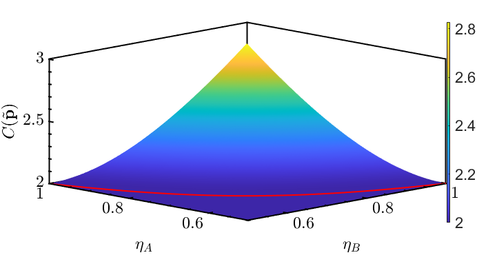
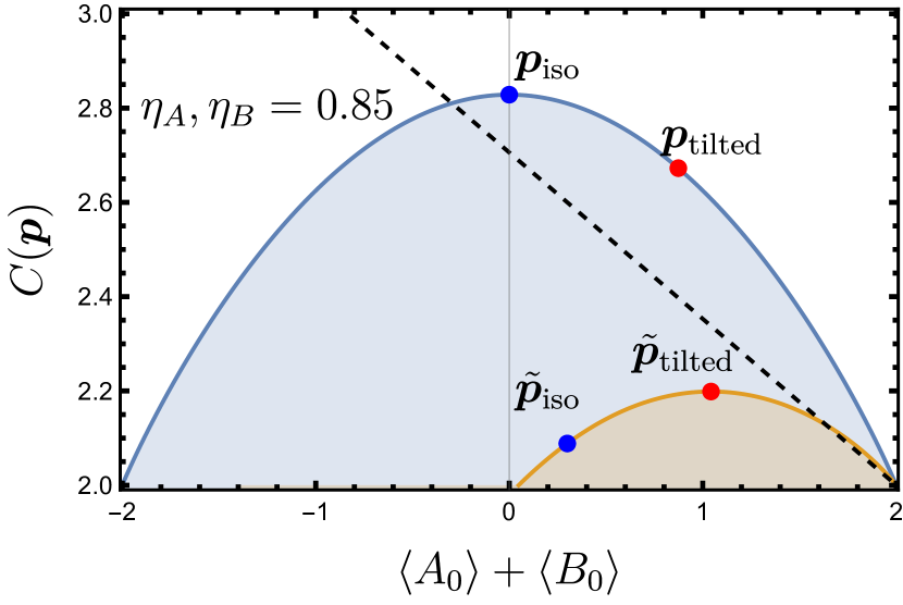
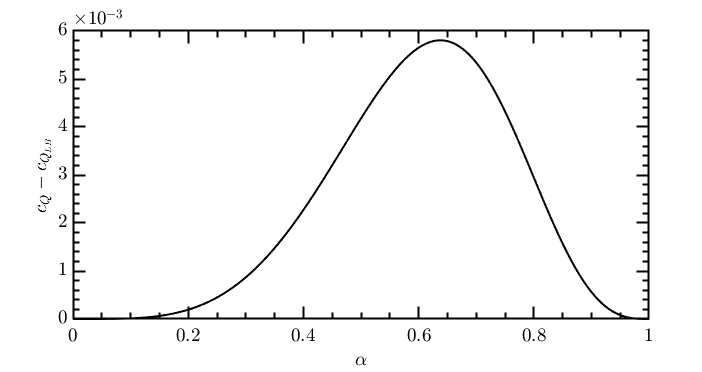
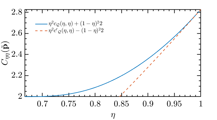
As discussed in the subsequent sections, retrieving the exact expression for the maximum violation of the doubly-tilted CHSH inequalities as a function of $\eta_{A},\eta_{B}$, with the traditional methods, such as the NPA hierarchy and SOS decompositions, turns out to be intractable. Despite this, in FIG 1, we plot the analytically obtained value of maximum loophole-free violation of the CHSH inequality against $\eta_{A},\eta_{B}\in[\frac{1}{2},1]$. Moreover, in FIG. 2, we use the optimal strategies to illustrate the effect of inefficient detectors with efficiency $\eta_{A}=\eta_{B}=0.85$ on the violation of CHSH inequality as a consequence of Lemma 1.

In the following sections, we describe the technique to retrieve the analytical expression and the analytical form of the optimal quantum strategies, which are self-tested by the maximal violation.

Figure 2: Effect of inefficient detectors on nonlocal correlations:— This graphic illustrates the impact of detector inefficiencies on nonlocal quantum correlations within the simplest Bell scenario. The blue region represents the set of quantum correlations $\bm{p}\in\mathcal{Q}$ in ideal conditions. With the detection efficiencies $\eta_{A}=\eta_{B}=0.85$, and the local assignement strategy $q_{A}(a|x)=\delta_{a,0},q_{B}(b|y)=\delta_{b,0}$, the effective quantum correlations $\tilde{\bm{p}}=\Omega_{\eta_{A}\eta_{B}}(\bm{p})$ are constrained to the smaller orange subset. The blue dot on the blue curve corresponds to the isotropic behavior $\bm{p}_{iso}$ that maximally violates the CHSH inequality, $C(\bm{p}_{iso})=2\sqrt{2}$, in ideal conditions, while the corresponding effective behavior (blue dot on the orange curve) $\tilde{\bm{p}}=\Omega_{\eta_{A}\eta_{B}}(\bm{p}_{iso})$ no longer attains the maximum loophole-free violation of the CHSH inequality, $C(\tilde{\bm{p}}_{tilted})\approx 2.08854$. Instead, the red dot on the blue curve corresponds to the quantum behavior $\bm{p}_{tilted}$ which maximally violates the doubly-tilted CHSH inequality (dashed black line), $C_{\eta_{A}\eta_{B}}(\bm{p}_{tilted})=2.98098$, (12), and attains the maximum loophole-free violation $C(\tilde{\bm{p}}_{tilted})\approx 2.19876$ (red dot on the orange curve) of the CHSH inequality, thereby, exemplifying Lemma 1.

IV SELF-TESTING OF CHSH INEQUALITIES TILTED FOR INEFFICIENT DETECTORS

In this section, we derive robust self-testing statements for the family of doubly-tilted CHSH inequalities (12), entailing the analytical expressions for the maximum violation, and the optimal quantum strategies. We briefly present the requisite preliminaries for self-testing by revisiting the already-solved sub-case of our problem, namely, CHSH inequalities tilted for one inefficient detector.

IV.1 One inefficient detector

Let us consider an ideal scenario wherein Alice has access to perfect detectors, such that $\eta_{A}=1$, while Bob’s detector are imperfect and click with efficiency $\eta_{B}$. Consequently, we retrieve the following family of completely asymmetrically tilted CHSH inequalities from (12),

$$C_{\alpha}(\bm{p})=\sum_{x,y}(-1)^{x\cdot y}\langle A_{x}B_{y}\rangle+\alpha\langle A_{0}\rangle\leq 2+\alpha,$$ (14)

where the tilting parameter $\alpha=\frac{2}{\eta_{B}}(1-\eta_{B})$ is determined by the detection efficiency on Bob’s side. First, from Observation 1 and (13), for quantum violation we have that $\eta_{B}\in(\frac{1}{2},1]$, which restricts the tilting parameter to $\alpha\in[0,2)$.

The maximum quantum value of the Bell functional in  (14) is $c_{\mathcal{Q}}(\alpha)=\sqrt{8+2\alpha^{2}}$ [19]. Hence, from (8), the maximum loophole-free violation of CHSH inequality when $\eta_{A}=1$ is $2\sqrt{2}\sqrt{\eta^{2}_{B}+(1-\eta_{B})^{2}}$. Recall that, in terms of the state and measurements $\{\ket{\psi^{\prime}},\hat{A}^{\prime}_{x},\hat{B}^{\prime}_{y}\}$ of an optimal quantum strategy, we can write the maximal functional value as $c_{\mathcal{Q}}(\alpha)=\langle\psi^{\prime}\hskip 1.0pt|\hskip 1.0pt\hat{C}_{\alpha}\hskip 1.0pt|\hskip 1.0pt\psi\rangle$, where $\hat{C}_{\alpha}$ is the CHSH Bell operator, given by

$$\hat{C}_{\alpha}=\sum_{x,y}(-1)^{x\cdot y}\hat{A}_{x}\otimes\hat{B}_{y}+\alpha\hat{A}_{0}.$$ (15)

In Ref. [18] it is shown that $\hat{C}_{\alpha}$ admits an SOS decompositions of the form

$$c_{\mathcal{Q}}(\alpha)\mathbb{1}-\hat{C}_{\alpha}=\sum_{i}P_{i}^{\dagger}P_{i},$$ (16)

in terms of polynomials $P_{i}$ in the operators $\{\mathbb{1},\hat{A}^{\prime}_{x},\hat{B}^{\prime}_{y},\hat{A}^{\prime}_{x}\otimes\hat{B}^{\prime}_{y}\}$. These decompositions are then used to prove that $c_{\mathcal{Q}}(\alpha)$ self-tests the optimal strategy $\{\ket{\psi},\hat{A}_{x},\hat{B}_{y}\}$ [18, 28], where

$$\begin{split}\ket{\psi}&=\cos{\theta}\ket{00}+\sin{\theta}\ket{11},\\ \hat{A}_{0}&=\sigma_{z}\qquad\hat{B}_{0}=\cos{\mu}\,\sigma_{z}+\sin{\mu}\,\sigma_{x}\\ \hat{A}_{1}&=\sigma_{x}\qquad\hat{B}_{1}=\cos{\mu}\,\sigma_{z}-\sin{\mu}\,\sigma_{x},\end{split}$$ (17)

with $\alpha=2/\sqrt{1+2\tan^{2}{2\theta}}$, $\tan(\mu)=\sin(2\theta)$ and $\sigma_{x(z)}$ denotes the $x(z)$ Pauli matrix.

The proof builds upon the observation that for any quantum strategy $\{\ket{\psi^{\prime}},\hat{A}^{\prime}_{x},\hat{B}^{\prime}_{y}\}$ attaining the value $c_{\mathcal{Q}}(\alpha)$, the SOS decomposition (16) implies that $\ket{\psi^{\prime}}$ must belong to the null space of the operators $P_{i}$, i.e., it must satisfy the conditions, $P_{i}\ket{\psi^{\prime}}=0$ for all $i$. From these conditions it is possible to infer the existence of operators $\{\hat{Z}_{A},\hat{X}_{A},\hat{Z}_{B},\hat{X}_{B}\}$ [18], such that,

$$\begin{split}\hat{Z}_{A}\ket{\psi^{\prime}}&=\hat{Z}_{B}\ket{\psi^{\prime}}\\ \sin\theta\hat{X}_{A}(\mathbb{1}+\hat{Z}_{B})\ket{\psi^{\prime}}&=\cos\theta\hat{X}_{A}(\mathbb{1}-\hat{Z}_{A})\ket{\psi^{\prime}}.\end{split}$$ (18)

The conditions (18) ensure the existence of local isometries, $\Phi_{A}$ and $\Phi_{B}$, mapping any optimal strategy $\{\ket{\psi^{\prime}},\hat{A}^{\prime}_{x},\hat{B}^{\prime}_{y}\}$ to the reference strategy $\{\ket{\psi},\hat{A}_{x},\hat{B}_{y}\}$ in (17), that is,

$$\begin{split}\Phi_{A}\otimes\Phi_{B}(\ket{\psi^{\prime}})&=\ket{\psi}\otimes\ket{\text{junk}}\\ \Phi_{A}\otimes\Phi_{B}(\hat{A}^{\prime}_{x}\otimes\hat{B}^{\prime}_{y}\ket{\psi^{\prime}})&=\hat{A}_{x}\otimes\hat{B}_{y}\ket{\psi}\otimes\ket{\text{junk}},\end{split}$$ (19)

where $\ket{\text{junk}}$ represents the arbitrary state of additional degrees of freedom on the which the measurements act trivially. Thus it is seen that the optimal quantum strategy is unique up to local isometries. We note that, while the proof of relations in Eq. (18) requires an ideal behavior, [18] demonstrates that the self-testing can be made robust. Recall, a Bell expression provides a robust self-test for a given quantum strategy, say $R$ if, in a noise-tolerant manner, the expected value $\beta$ in close to the maximum $\beta_{\mathcal{Q}}$ consistently corresponds to a strategy $\tilde{R}$ in a close neighbourhood of the reference strategy $R$, up to local isometries.

Let us now proceed to the unsolved general case of inefficient detectors for both parties.

IV.2 Two inefficient detectors

We now consider the most generic experimental setting, wherein the detectors of both parties may be imperfect and click with efficiencies $\eta_{A},\eta_{B}\in[0,1]$. We rewrite for convenience, the doubly-tilted CHSH inequalities (12) for the general case as,

$$C_{\alpha,\beta}(\bm{p})=\sum_{x,y}(-1)^{x\cdot y}\langle A_{x}B_{y}\rangle+\alpha\langle A_{0}\rangle+\beta\langle B_{0}\rangle\leq 2+\alpha+\beta,$$ (20)

where the tilting parameter $\alpha=\frac{2}{\eta_{B}}(1-\eta_{B})$ for Alice’s term $\langle A_{0}\rangle$ depends on the Bob’s detection efficiency $\eta_{B}$, while Bob’s tilting parameter $\beta=\frac{2}{\eta_{A}}(1-\eta_{A})$ is determined by Alice’s efficiency $\eta_{A}$. Consequently, the boundary of the region of interest (13) translates to $0<\alpha+\beta<2$, in terms of the tilting parameters. We are interested in finding the maximal violation of the inequality in (20), as well as a quantum state and measurements attaining it, as a function of the tilting parameters $\alpha,\beta$. However, we find the problem to be intractable via analytical techniques described above. In what follows we first describe in more detail the difficulties that arise when trying to obtain a tight SOS decomposition for the Bell operator on the left of (20), and then we show that obtaining an analytical solution is nonetheless possible by a different technique.

IV.2.1 Impracticality of the SOS technique and NPA upper-bound convergence

Before we derive the analytical expression for the maximal quantum violation $c_{\mathcal{Q}}(\alpha,\beta)$ of the doubly-tilted CHSH inequality (12) with an alternative technique, here we demonstrate that the standard SOS decomposition technique, though theoretically applicable, becomes impractical for these inequalities.

The problem of finding the maximum quantum violation $\beta_{\mathcal{Q}}$ of a Bell inequality (2) can be relaxed with the NPA hierarchy [29] of semi-definite programs. Specifically, the NPA hierarchy returns a converging sequence of upper-bounds $\beta_{\mathcal{Q}_{L}}$ on the maximum quantum violation $\beta_{\mathcal{Q}}$. Here, $L\in\{1,1+AB,2,\ldots\}$ denotes the level of the hierarchy, which corresponds to the length of the monomials of the measurement operators $\{\hat{M}_{a}^{x},\hat{N}_{b}^{y}\}$. We recall that finding a tight upper bound on the maximum quantum violation of Bell inequalities using NPA hierarchy, such that $\beta_{\mathcal{Q}_{L}}=\beta_{\mathcal{Q}}$, and retrieving a tight SOS decomposition $\sum_{i}P_{i}^{\dagger}P_{i}$ for the operator $\beta_{\mathcal{Q}}\mathbb{I}-\hat{\beta}$ form a primal-dual pair of SDPs, where $P_{i}$ are polynomials in the optimal measurement operators $\{\hat{M}_{a}^{x},\hat{N}_{b}^{y}\}$. In particular, the level $L$ of the NPA hierarchy at which $\beta_{\mathcal{Q}}=\beta_{\mathcal{Q}}$ corresponds to the degree of the polynomials $P_{i}$ in a tight SOS decomposition. For instance, the degree polynomials in the tight SOS decompositions (16) of the completely asymmetrically doubly-tilted CHSH inequalities reflect the fact that the level $1+AB$ of the NPA hierarchy is sufficient to retrieve the maximum quantum violation for these inequalities.

Figure 3: Increasing levels for tight NPA upper bounds in the CHSH scenario:— A plot of the minimum level $L\in\{1,1+AB,2,3,4,5,6,7+\}$ of the NPA hierarchy required to saturate (up to machine precision) the maximum quantum violation $c_{\mathcal{Q}}(\alpha,\beta)$ for $\alpha,\beta\in[0,2]$. Notably, the required minimum level of the NPA-hierarchy rapidly increases as the tilting parameters the critical boundary $\alpha+\beta=2$.

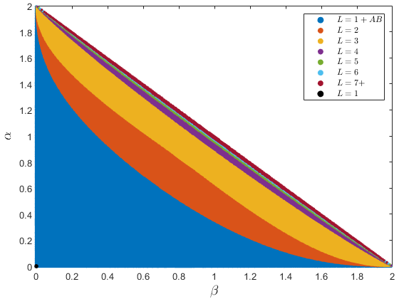
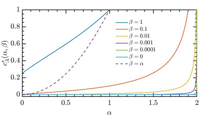
In FIG. 3, we chart the minimum level $L$ of the NPA hierarchy against the tilting parameters $\alpha,\beta$ required to saturate the maximum quantum violation $c_{\mathcal{Q}}(\alpha,\beta)$ (found in the next section) of doubly-tilted CHSH inequalities (20), up to machine precision. Remarkably, as the tilting parameters $\alpha,\beta$ approach the critical boundary (13), $\alpha+\beta=2$, the level $L$ of NPA hierarchy increases rapidly. In particular, we found that even the level $12$ of the NPA hierarchy is not enough to saturate the maximum violation of the symmetrically doubly-tilted CHSH inequality when $\alpha=\beta=0.999$. This observation raises a critical question: is any finite level of the NPA hierarchy enough to saturate the maximum quantum violation of the doubly-tilted CHSH inequalities for all tilting parameters $\alpha,\beta$? The uncertainty surrounding this question implies that the degree of polynomials required for a tight analytical SOS decomposition for these inequalities remains elusive and potentially unbounded.

Nonetheless, for a significantly large range of the parameters $\alpha,\beta$, the NPA level $1+AB$ saturates the maximum quantum violation $c_{\mathcal{Q}}(\alpha,\beta)$. This observation makes it tempting to apply the methodology from [18] to extend the analytical self-testing results by finding a Sum-of-Squares (SOS) decomposition for the Bell operator $\hat{C}_{\alpha\beta}$ associated with the general doubly-tilted CHSH inequalities. Indeed, it is possible to numerically retrieve SOS decompositions for fixed values of the tilting parameters, especially when lower levels of NPA hierarchy saturate the maximum quantum violation. However, unlike the simpler completely asymmetric where the SOS decomposition includes just two polynomials, even the simplest decompositions for the general case demand at least five polynomials. The task of deducing a generically applicable analytical SOS decomposition from the numerical results is significantly hindered due to the complex dependence of the maximal quantum violation and the optimal quantum strategy on the tilting parameters $\alpha,\beta$. This complex interdependence translates into the SOS polynomials, rendering them overly convoluted and preventing any definitive statements about the optimal strategies based on the SOS decompositions. Interestingly, nonetheless, for the symmetric case with $\alpha=\beta=2/\sqrt{13}$, it is possible to find the analytical expression of the polynomials of degree $1+AB$ in the tight SOS decomposition and the optimal quantum strategy.

(a)

(b)

Figure 4: Error in estimation of maximum quantum violation:— The curves in plot (a) correspond to the difference $c_{\mathcal{Q}_{L}}(\alpha,\alpha)-c_{\mathcal{Q}}(\alpha,\alpha)$ ($\times 10^{-8}$) between the upper-bounds from the levels $L\in\{7,8,9,10\}$ of the NPA hierarchy and the maximum quantum violation $c_{\mathcal{Q}}(\alpha,\alpha)$ of symmetrically tilted Bell inequalities (12), against $\alpha\in[0.99,1]$, obtained with an arbitrary precision solver SDPA-GMP [32] and our analytical solution (Theorem 1), respectively. This plot demonstrates the insufficiency of high levels of the NPA hierarchy for obtaining tight bounds in the CHSH scenario. The curve in plot (b) corresponds to the difference $c_{\mathcal{Q}}(\alpha,\alpha)-c_{\mathcal{Q}_{LB}}(\alpha,\alpha)$ ($\times 10^{-3}$) between the maximum quantum violation $c_{\mathcal{Q}}(\alpha,\alpha)$ and the lower-bound $c_{\mathcal{Q}_{LB}}(\alpha,\alpha)$ corresponding to the sub-optimal analytical solutions presented in [13], against $\alpha\in[0,1]$.

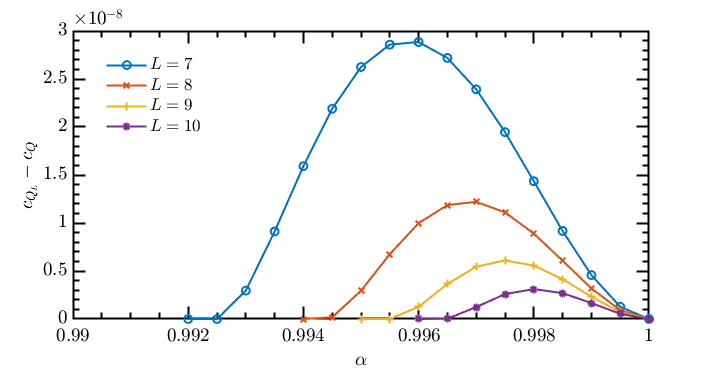
The derivation of the self-testing results presented in the section IV.1, relied heavily on the existence of SOS decompositions from which relations of the form $P_{i}\ket{\psi}=0$, where $\{P_{i}\}$ are polynomial functions on the measurement operators of an optimal realization $\{\hat{A}_{x},\hat{B}_{y},\ket{\psi}\}$. The increase in the minimum degree as well as the number of polynomials in tight SOS decomposition for the general tilted-Bell inequalities, makes self-testing with the SOS technique for general doubly-tilted CHSH inequalities too arduous to be practical. Nevertheless, as we show in the next section, it is still possible to retrieve the analytical expressions for the maximum quantum violation and the optimal quantum strategy for general doubly-tilted CHSH inequalities and demonstrate that the maximum violation self-tests the optimal quantum strategy.

IV.2.2 Self-testing based on Jordan’s lemma

Lacking tight analytical SOS decompositions for the general doubly-tilted CHSH inequalities (20), we present in this section an alternative approach based on Jordan’s lemma [33, 34, 35].

Jordan’s lemma provides a convenient characterization for the local observables of a party having two settings with two outputs each. In particular, in CHSH scenario, we can take Alice and Bob’s observables $A_{x},B_{y}$ to be projective, à la Naimark’s dilation theorem. Jordan’s lemma then asserts that there exists local unitary transformations that simultaneously block-diagonalise the observables $A_{x},B_{y}$, with one and two dimensional blocks. As we are interested in the expectation values $\langle\hat{A}_{x}\rangle,\langle\hat{B}_{y}\rangle$ of the observables with respect to a state $\ket{\psi}$, we can always add a projector $|\hskip 1.0pt\phi\rangle\langle\phi\hskip 1.0pt|$ onto the $\operatorname{Ker}(\rho_{A})$ of the respective reduced state $\rho_{A}=\Tr_{B}{|\hskip 1.0pt\psi\rangle\langle\psi\hskip 1.0pt|}$ to each one dimensional block. Hence, we can, without loss of generality, take all Jordan blocks to be two-dimensional, such that Alice’s observables can now be expressed as,

$$\hat{A}_{0} =\bigoplus_{i}\hat{A}^{(i)}_{0}=\bigoplus_{i}{\sigma}_{Z}$$ (21)

$$\hat{A}_{1} =\bigoplus_{i}\hat{A}^{(i)}_{1}=\bigoplus_{i}(\cos{\theta_{i}^{A}}\,{\sigma}_{Z}+\sin{\theta_{i}^{A}}\,{\sigma}_{X}),$$ (22)

where the index $i$ iterates runs over blocks and $\sigma^{(i)}_{Z},\sigma^{(i)}_{X}$ denote the Pauli $Z,X$ matrices on the $i$th two dimensional block. Similarly, Bob’s observables can be expressed as,

$$\hat{B}_{0} =\bigoplus_{j}\hat{B}^{(j)}_{0}=\bigoplus_{j}{\sigma}_{Z}$$ (23)

$$\hat{B}_{1} =\bigoplus_{j}\hat{B}^{(j)}_{1}=\bigoplus_{j}(\cos{\theta_{j}^{B}}\,{\sigma}_{Z}+\sin{\theta_{i}^{B}}\,{\sigma}_{X}),$$ (24)

where again $j$ runs over blocks. Consequently, the Bell operator $\hat{C}_{\alpha\beta}$ associated with the general doubly-tilted CHSH inequalities (20) also take a block diagonal form,

$$\hat{C}_{\alpha\beta}=\sum_{i,j}\hat{C}_{\alpha\beta}(\theta_{i}^{A},\theta_{j}^{B}),$$ (25)

where $\hat{C}_{\alpha\beta}(\theta_{i}^{A},\theta_{j}^{B})$ is an operator with local dimension $2$ given by

$$\hat{C}_{\alpha\beta}(\theta_{i}^{A},\theta_{j}^{B})=\sum_{x,y}(-1)^{x\cdot y}\hat{A}^{(i)}_{x}\otimes\hat{B}^{(j)}_{y}\\ +\alpha(\hat{A}^{(i)}_{0}\otimes\mathbb{I}_{2})+\beta(\mathbb{I}_{2}\otimes\hat{B}^{(j)}_{0}).$$ (26)

where $\mathbb{1}_{2}$ denotes the two-dimensional identity operator.

Let $\Pi_{i},\Pi_{j}$ be the projectors onto Alice’s $i$th and Bob’s $j$th blocks respectively, such that, $\hat{C}_{\alpha\beta}(\theta_{i}^{A},\theta_{j}^{B})=\Pi_{i}\otimes\Pi_{j}\hat{C}_{\alpha,\beta}\Pi_{i}\otimes\Pi_{j}$. Consequently, the value of the Bell functional $C_{\alpha\beta}(\bm{p})$ is given by

$$C_{\alpha\beta}(\bm{p})=\expectationvalue{\hat{C}_{\alpha\beta}}_{\ket{\psi}}=\sum_{i,j}p_{ij}\tr{\rho_{ij}\hat{C}_{\alpha\beta}(\theta_{i}^{A},\theta_{j}^{B})},$$ (27)

where $p_{ij}\,\rho_{ij}=(\Pi_{i}\otimes\Pi_{j})|\hskip 1.0pt\psi\rangle\langle\psi\hskip 1.0pt|(\Pi_{i}\otimes\Pi_{j})$ are the (unnormalised) projections of $\ket{\psi}$ onto the $i$th and $j$th blocks of Alice and Bob, respectively. Since $C_{\alpha\beta}(\bm{p})$ is a convex combination of the values $\tr{\rho_{ij}\hat{C}_{\alpha\beta}(\theta_{i}^{A},\theta_{j}^{B})}$ in Alice’s $i$th and Bob’s $j$th blocks with weights $p_{ij}$, its maximum value $c_{\mathcal{Q}}(\alpha,\beta)$ is attained when for all $i$, $j$, the value of the Bell functional is the optimal two–qubit value. Consequently, without loss of generality,

$$\hat{A}_{0} ={\sigma}_{Z}\ ,\ \hat{A}_{1}=c_{A}\,{\sigma}_{Z}+s_{A}\,{\sigma}_{X}$$ (28a)

$$\hat{B}_{0} ={\sigma}_{Z}\ ,\ \hat{B}_{1}=c_{B}\,{\sigma}_{Z}+s_{B}\,{\sigma}_{X},$$ (28b)

where $c_{A}=\cos\theta_{A}$, $s_{A}=\sin\theta_{A}$, $c_{B}=\cos\theta_{B}$ and $s_{B}=\sin\theta_{B}$. Consequently, the maximum quantum violation ${c}_{\mathcal{Q}}(\alpha,\beta)$ self-tests a quantum strategy if, up to local two-dimensional unitaries, the optimal two-qubit strategy is unique. Now we are prepared to present our main result, namely, the analytical self-testing statements for the symmetrically ($\alpha=\beta$) tilted CHSH inequality. We have differed the self-testing statements for the general case of $\alpha\neq\beta$ to the supplementary material (Sec. B) for brevity.

Theorem 1.

[Self-testing of symmetrically tilted CHSH inequalities] The maximum quantum violation $c_{\mathcal{Q}}(\alpha,\alpha)$ of the symmetrically $(\alpha=\beta)$ tilted CHSH inequality (12) is the largest root of the degree 4 polynomial,

$$f(\lambda)=\lambda^{4}+(4-\alpha^{2})\lambda^{3}+\left(\frac{11}{4}\alpha^{4}-12\alpha^{2}-4\right)\lambda^{2}\\ +(2\alpha^{6}-\alpha^{4}-20\alpha^{2}-32)\lambda+5\alpha^{6}-21\alpha^{4}+16\alpha^{2}-32.$$ (29)

$C_{\alpha\alpha}(\bm{p})=c_{\mathcal{Q}}(\alpha,\alpha)$ self-tests a two qubit quantum strategy with optimal $(*)$ local observables of the form (28), such that the optimal cosines are equal, i.e., ${c}^{*}(\alpha)=c^{*}_{A}(\alpha)=c^{*}_{B}(\alpha)\in[0,1]$, and satisfy the relation,

$${c}^{*}(\alpha)=\frac{1}{8}\left[3\alpha^{2}-4+\sqrt{16+9\alpha^{4}+8\alpha^{2}(2c_{\mathcal{Q}}(\alpha,\alpha)-1)}\right].$$ (30)

Proof.

Here, we present a comprehensive overview of the proof-technique while the complete proof is contained in the accompanying Mathematica notebook. As discussed above Jordan’s lemma lets us express the Bell operator $\hat{C}_{\alpha\beta=\alpha}$ associated with the symmetrically $(\alpha=\beta)$ tilted CHSH inequality (12) as a two qubit operator,

$$\hat{C}_{\alpha\alpha}=\sum_{x,y}(-1)^{x\cdot y}\hat{A}_{x}\otimes\hat{B}_{y}+\alpha(\hat{A}_{0}\otimes\mathbb{I}_{2}+\mathbb{I}_{2}\otimes\hat{B}_{0}).$$ (31)

With the parametrization (28), the Bell operator $\hat{C}_{\alpha\alpha}$, now a function of just two cosines $c_{A},c_{B}\in[0,1]$, has the following four dimensional matrix representation:

$$\left(\begin{array}[]{cccc}\omega+2\alpha&s_{B}-c_{A}s_{B}&s_{A}-c_{B}s_{A}&-s_{A}s_{B}\\ s_{B}-c_{A}s_{B}&-\omega&-s_{A}s_{B}&(c_{B}-1)s_{A}\\ s_{A}-c_{B}s_{A}&-s_{A}s_{B}&-\omega&(c_{A}-1)s_{B}\\ -s_{A}s_{B}&(c_{B}-1)s_{A}&(c_{A}-1)s_{B}&\omega-2\alpha\\ \end{array}\right)$$ (32)

where $\omega=1+c_{A}+c_{B}-c_{B}c_{A}$. Now, for fixed cosines $c_{A},c_{B}$, the maximum quantum violation $c_{\mathcal{Q}}(\alpha,\alpha)$ of the symmetrically doubly-tilted CHSH inequality corresponds to the largest eigenvalue of the matrix (32), i.e., the largest root of its characteristic polynomial $q(\lambda,c_{A},c_{B},\alpha)$, which has the form,

$$q(\lambda,c_{A},c_{B},\alpha)= \lambda^{4}-(4\alpha^{2}+8)\lambda^{2}$$

$$+ 8\alpha^{2}(c_{A}c_{B}-c_{A}-c_{B}-1)\lambda$$

$$+ 8[2(c_{B}^{2}+c_{A}^{2}(1-c_{B}^{2}))-\alpha^{2}(c_{A}^{2}(1-c_{B}))$$

$$+c_{B}(1+c_{B})-c_{A}s_{B}(1-c_{B}^{2})],$$ (33)

where $\lambda$ denotes the eigenvalue of the matrix (32). Thus, finding $c_{\mathcal{Q}}(\alpha,\alpha)$ boils down to maximizing the largest root of $q(\lambda,c_{A},c_{B},\alpha)$ in (33) over the cosines $c_{A}$ and $c_{B}$. While for any fixed value of the tilting parameter $\alpha$, this optimization problem can be numerically solved, obtaining an analytical expression as a function of the $\alpha$ is a more arduous problem. We now describe how such expression can be obtained via Gröbner basis elimination for both the optimal quantum value $c_{\mathcal{Q}}(\alpha,\alpha)$ and the optimal measurement settings in terms of cosines $c^{*}_{A}(\alpha),c^{*}_{B}(\alpha)$.

Let us consider the Lagrangian for this problem,

$$L=\lambda+s\cdot q(\lambda,c_{A},c_{B},\alpha)$$ (34)

where $s$ is a Lagrange multiplier. Consequently, the stationary points must satisfy the conditions, $\partial_{c_{A}}L=\partial_{c_{B}}L=\partial_{s}L=0$, which in-turn imply the following polynomial conditions,

$$\left\{\begin{aligned} q(\lambda,c_{A},c_{B},\alpha)&=0\\ q_{c_{A}}(\lambda,c_{A},c_{B},\alpha)&=\partial_{c_{A}}q(\lambda,c_{A},c_{B},\alpha)=0\\ q_{c_{B}}(\lambda,c_{A},c_{B},\alpha)&=\partial_{c_{B}}q(\lambda,c_{A},c_{B},\alpha)=0.\end{aligned}\right.$$ (35)

The cosines parameterizing the optimal observables ${c}_{A}^{*}(\alpha),{c}_{B}^{*}(\alpha)$ and the maximum quantum violation $c_{\mathcal{Q}}(\alpha,\alpha)={\lambda}^{*}(\alpha)$ are thus common roots of the polynomials $q,q_{c_{A}},q_{c_{B}}$ in (35). We now use the Gröbner basis elimination on $q,q_{c_{A}},q_{c_{B}}$ to eliminate the cosines $c_{A},c_{B}$ and retrieve a polynomial $f_{0}(\lambda)$ of degree 12. We then take the polynomial quotient of $f_{0}(\lambda)$ with respect to eight trivial and sub-optimal roots to retrieve the desired degree 4 polynomial $f(\lambda)$ (29). The expression for maximum quantum violation $c_{\mathcal{Q}}(\alpha,\alpha)$ which corresponds to the largest real root of the polynomial $f(\lambda)$ as a function of $\alpha$ is contained in the accompanying Mathematica notebook (See FIG. 1 in the more general scenario $\eta_{A}\neq\eta_{B}$).

Similarly, to find the expression for Alice’s optimal cosine ${c}_{A}^{*}(\alpha)$, we eliminate ${c}_{B},\lambda$ using Gröbner basis elimination on $q,q_{c_{A}},q_{c_{B}}$. This results in a degree 11 polynomial $g_{0}(c)$. We then take the polynomial quotient of $g_{0}(c)$ with respect to seven trivial and sub-optimal roots to obtain the following degree 4 polynomial,

$$g(c)=-16c^{4}+\left(40\alpha^{2}-32\right)c^{3}\\ +\left(-33\alpha^{4}+48\alpha^{2}-16\right)c^{2}+\left(8\alpha^{6}-10\alpha^{4}+8\alpha^{2}\right)c\\ -4\alpha^{6}+7\alpha^{4}$$ (36)

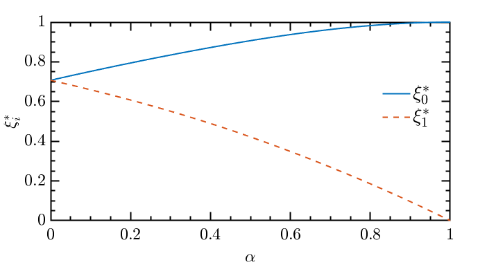
Repeating the same procedure for Bob’s optimal cosine ${c}_{B}^{*}(\alpha)$, we end up with a degree 4 polynomial identical to $g(c)$ in (36). We find the expressions for the optimal cosines to be identical ${c}_{A}^{*}(\alpha)={c}_{B}^{*}(\alpha)={c}^{*}_{\alpha}$ and corresponding to the largest root ${c}^{*}_{\alpha}$ of $g(c)$ (contained accompanying Mathematica notebook and see FIG. 5 for the scenario $\alpha\neq\beta$). Furthermore, the simplification ${c}_{A}^{*}(\alpha)={c}_{B}^{*}(\alpha)={c}^{*}_{\alpha}$ allows us to derive the relation (30) between the maximum quantum violation $c_{\mathcal{Q}}(\alpha,\alpha)$ and the optimal cosine ${c}^{*}_{\alpha}$. Observe that in the interval $[0,\pi]$ the angle $\theta^{*}_{A}=\theta^{*}_{B}=\theta$ between optimal measurements is uniquely determined by $c_{\mathcal{Q}}(\alpha,\alpha)$ via the relation (30), and therefore, the measurements in the optimal two-qubit realization are unique up to local unitaries. Thus, the maximum quantum violation of symmetrically doubly-tilted CHSH inequalities self-tests the optimal measurements. Since the largest eigenvalue of the Bell operator with the optimal measurements is non-degenerate, the maximum quantum violation $c_{\mathcal{Q}}(\alpha,\alpha)$ also self-tests the state partially entangled two-qubit state which corresponding to eigenvector associated with the largest eigenvalue (see FIG. 6). ∎

The presented self-testing results rely on ideal experimental conditions. In the next section, we demonstrate the robustness of these results, showing that small deviations from the maximal violation limit the variation from the optimal realization. In the last section, we discuss several key insights based on the self-testing results derived in this section.

Figure 5: Self-testing of partially incompatible observables:— A plot of the optimal cosines of Alice $c^{*}_{A}(\alpha,\beta)$ (28) with $\beta\in\{\alpha,0.1,0.01,0.001,0\}$ self-tested by the maximum quantum violation $C_{\alpha\beta}(\bm{p})=c_{Q}(\alpha,\beta)$ of the doubly-tilted CHSH inequalities (12) against the tilting parameter $\alpha\in[0,1]$. Here, $c^{*}_{A}(\alpha,\beta)=0$ implies maximally incompatible whereas $c^{*}_{A}(\alpha,\beta)=1$ reflects compatible observables. Notice, that in contrast to the totally asymmetrically case $\beta=0$ wherein Alice’s optimal cosine $c^{*}_{A}(\alpha,\beta=0)$ stays constant with respect to $\alpha$ [18], for the general case, whenever $\beta>0$, Alice’s optimal measurements change with $\alpha=\frac{2}{\eta_{B}}(1-\eta_{B})$ and in-turn depend on Bob’s detection efficiency $\eta_{B}$, and tend towards compatible measurements as $\alpha\to 2-\beta$.

Figure 6: Self-testing of non-maximally entangled states:— A plot of the Schmidt coefficients $\xi^{*}_{i}$ of the optimal non-maximally entangled quantum state $\ket{\psi}=\xi^{*}_{0}\ket{00}+\xi^{*}_{1}\ket{11}$ (represented in the Schmidt basis) against $\alpha\in[0,1]$ for attaining maximum quantum violation of the symmetrically ($\alpha=\beta$) tilted CHSH inequality (12). Notice, as $\alpha=\beta\to 1$ ($\eta\to\frac{2}{3}$) the optimal state becomes almost product.

IV.2.3 Robust self-testing

The self-testing statements derived in this work rely on the assumption that the violation of the given Bell inequality is maximal, which is an theoretically idealization due to the inevitability of experimental imperfections. Therefore, the self-testing results must be made robust. The lack an analytical tight SOS decomposition prevents us from studying the robustness of these self-testing results analytically. Nevertheless, we can approach this problem by means of the numerical SWAP technique introduced in [36, 37].

Figure 7: Robustness of the self-testing statements:— A plot of lower bounds $\mathcal{F}^{*}_{L}$ on the minimum quantum fidelity $\mathcal{F}_{L}^{*}\leq\mathcal{F}^{*}$ from the level $L=3$ of NPA hierarchy between the actual state and the optimal self-testing state against the violation $C_{\alpha\alpha}(\bm{p})$ of the symmetrically ($\alpha=\beta$) tilted CHSH inequality (12) for tilting parameters $\alpha\in\{0.3,0.4,0.5,0.6,0.7,0.8\}$.

The numerical SWAP method utilizes the NPA hierarchy to obtain lower bounds on the closeness (fidelity) of the experimental measurements and the shared state to the ideal self-testing measurements and state. Here we describe the technique for bounding the fidelity between any optimal state $\ket{\psi^{\prime}}$ and the reference self-testing state $\ket{\psi}$. The main idea of this technique relies on the notion of local isometries, which map the actual physical state $\ket{\psi^{\prime}}$ to our reference self-testing state $\ket{\psi}$ and a junk state $\ket{\text{junk}}$ on auxiliary local degrees of freedom. In particular, the local isometries act as partial SWAP gates, essentially swapping the actual physical state $\ket{\psi^{\prime}}$ with the state $\ket{0}^{\otimes N}$ of the registers, such that the final state of the registers corresponds to the reference self-testing state $\ket{\psi}$. The local isometries can be implemented through a SWAP circuit $U_{SWAP}$, such that the fidelity $\mathcal{F}=\bra{\psi}U_{SWAP}\ket{\psi^{\prime}}=1$ for any state $\ket{\psi^{\prime}}$ maximally violating the Bell inequality.

Consequently, we can cast the problem of certifying whether the behavior $\bm{p}$ attaining maximum violation of a Bell inequality self-tests the optimal state $\ket{\psi}$, as that of minimising the fidelity $\mathcal{F}$, with the behavior subject to the behavior $\bm{p}$ admitting a quantum strategy. While this optimisation problem is in general computationally hard, we can relax it as a semidefinite program (SDP) via the NPA hierarchy.

The SWAP circuit $U_{SWAP}$ only depends on the self-testing measurements. The particulars of such $U_{SWAP}$, specifically those corresponding local isometries, enable us to express the fidelity, $\mathcal{F}_{L}=\expectationvalue{\rho_{SWAP}(\Gamma_{L})}{\psi}$, of the final state of the register $\rho_{SWAP}(\Gamma_{L})$ with the reference state $\ket{\psi}$, as a function of the entries of the necessarily positive semi-definite NPA moment matrix $\Gamma_{L}$ of level $L$, as well as of the reference self-testing state $\ket{\psi}$. As some of the entries of the moment matrix $\Gamma_{L}$ correspond to experimental behavior, such as $[\Gamma_{n}]_{\hat{A}_{x}^{\prime},\hat{B}_{y}^{\prime}}=\expectationvalue{\hat{A}_{x}^{\prime}\hat{B}_{y}^{\prime}}{\psi^{\prime}}$, the behavioral preconditions of a self-testing statement translate to linear constraints on the entries of the moment matrix $\Gamma_{L}$. Given a target self-testing state $\ket{\psi}$ and solving the consequent semi-definite minimization program with the fidelity, $\mathcal{F}_{L}=\expectationvalue{\rho_{SWAP}(\Gamma_{L})}{\psi}$ as the linear objective function, retrieves a converging sequence of lower bounds, $\mathcal{F}^{*}_{1}\leq\mathcal{F}^{*}_{2}\leq\ldots\leq\mathcal{F}^{*}_{L}$ such that $\mathcal{F}^{*}_{L\to\infty}=\mathcal{F}^{*}$, on the minimal quantum fidelity $\mathcal{F}^{*}$.

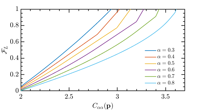
In the figure FIG. 7, we plot a lower bound of the minimal fidelity $\mathcal{F}^{*}_{L}$ against the violation of the symmetrically tilted Bell inequality $C_{\alpha\alpha}(\bm{p})$, for $\alpha\in\{0.2,0.4,0.6,0.8\}$ obtained with the numerical SWAP method. For these curves, for each $\alpha$, we used the maximal violation of the doubly-tilted CHSH inequality  (20), and the reference optimal state and measurements, derived in the previous section. Since the optimal observables $\hat{A}_{1}$ and $\hat{B}_{1}$ are given by some linear combination of gates $\hat{Z}$ and $\hat{X}$ in the SWAP circuit, to find the minimum fidelity $\mathcal{F}_{L}$, we introduce extra dichotomic operators $\hat{A}_{2}$ and $\hat{B}_{2}$ to account for the $X$ gate on Alice’s and Bob’s side and impose the relevant extra constraints by means of localising matrices [36].

We find that level $3$ of the NPA hierarchy is enough for producing the fidelity curves for $\alpha<0.9$, but higher values of $\alpha$ require increasing levels of the hierarchy. We tentatively attribute this effect to the exploding levels of the NPA hierarchy described in the section IV.2.1. Observe that the minimal fidelity becomes $\mathcal{F}_{L}=\mathcal{F}=1$ when the inequality violation is maximal, indicating that the maximal quantum violation self-tests the optimal state, as expected from the discussion above. In particular, for $\alpha>0.3$ a clear change in behavior in the fidelity curve is observed when the violation reaches the maximal local value $C_{\alpha\alpha}(\bm{p})=2+2\alpha$, after which the dependence is almost linear.

V Discussions

The experimental realization of long-range loophole-free nonlocal correlations is a prerequisite for the large-scale adoption of device-independent quantum cryptography. However, a significant hurdle stands in our way: the inevitable loss of photons in optical fibers and the limited efficiencies of detectors. In particular, if the detection efficiencies fall below the critical value, the otherwise nonlocal quantum strategies cease to produce nonlocal correlations. Consequently, extensive research has thus far been devoted to identifying quantum strategies with minimal threshold detection efficiencies. Nonetheless, there is a distinct but significant unaddressed question: what quantum strategies maximize loophole-free nonlocality when detector efficiencies surpass these critical values?

In this work, we addressed the problem of finding the quantum strategies that maximize the loophole-free violation of a given Bell inequality in the presence of inefficient detectors. In Lemma 1, we demonstrate that for any Bell inequalities and any specification of detection efficiencies, the quantum strategies that yield the maximum loophole-free violation are the ones that maximally violate a tilted version of the Bell inequality. We then focus on the simplest case of the CHSH inequality (10) to retrieve a family of doubly-tilted CHSH inequalities (12). As our main results, we derive analytical self-testing statements (Theorem 1 ) for this family of Bell inequalities, entailing the analytical expressions for the maximum quantum violation and the ensuing optimal quantum strategy. In particular, we note that the maximum violation of the tilted CHSH inequality in Theorem 1 differs from that reported in [13] (see FIG. 4). Additionally, it is worth noting that the nonlocal correlations maximally violating the tilted inequalities in (7) also maximize the guessing probability $\expectationvalue{A_{0}}+\expectationvalue{B_{0}}$, subject to the given CHSH functional value $C(\bm{p})$. Consequently, the quantum strategies obtained via Theorem 1 allow us to recover the boundary of the set of quantum correlations on the slice $C(\bm{p})$ vs $\expectationvalue{A_{0}}+\expectationvalue{B_{0}}$, plotted in FIG. 2. Furthermore, these quantum strategies have found application in the recently introduced routed Bell experiments [14, 38, 39].

Besides providing a convenient way for finding quantum strategies that generate the maximum loophole-free nonlocality, Lemma 1, and in particular the expression of the tilted Bell inequalities (7), offers crucial insights into the how the optimal quantum behaviors move with the efficiencies of the detectors in the no-signaling polytope. Essentially, with decreasing efficiencies, the hyperplane corresponding to the Bell inequality (7) tilts about a local deterministic point specified by the assignment strategies, in turn moving the optimal strategies along towards the local polytope $\mathcal{L}$, and specifically towards the local deterministic point. We exemplify this observation in FIG. 2.

The family of self-testing statements in Theorem 1 and 2 provide crucial insights into how decreasing detector efficiency affects optimal quantum strategies. As illustrated in figure 6, for inefficient detectors $\eta_{A},\eta_{B}<1$ ($\alpha,\beta>0$), the optimal strategy requires partially entangled states for maximal loophole-free nonlocality. Observe that the degree of entanglement decreases as the efficiencies approach the critical values (13), as the state becomes almost product. While this finding is in line with observations from the known asymmetric case $\eta_{A}=1$ ($\beta=0$), the optimal measurements present an intriguing deviation. Specifically, in the asymmetric case $\eta_{A}=1$ ($\beta=0$) (17), Alice’s optimal measurements remain maximally incompatible irrespective of Bob’s detection efficiency $\eta_{B}\in(1/2,1]$ ($\alpha\in[0,2)$), while Bob requires partially incompatible measurements whose incompatibility decreases with his decreasing efficiency $\eta_{B}$ ($\alpha$), approaching almost compatible measurements as $\eta_{B}\to 1/2$ ($\alpha\to 1$). However, the situation changes significantly when both detectors are inefficient. As we illustrate in FIG. 5, in contrast to the asymmetric case, Alice’s measurements depend non-trivially on Bob’s detection efficiency $\eta_{B}$. Specifically, whenever $\eta_{A}<1$ ($\beta>0$), Alice’s optimal measurement tends towards compatible measurements as $\eta_{B}$ ($\alpha$) approaches the critical boundary ($\alpha\to 2-\beta$) (13). This observation highlights the natural importance of partially incompatible measurements in device independent cryptography [40]. Finally, as Bell scenarios are linked to prepare and measure scenarios [41], it would be interesting to investigate the implications of our results to prepare and measure experiments with inefficient detectors.

Besides the inferences concerning the maximum effective nonlocality in the presence of inefficient detectors, the analytical results in Theorem 1 and 2 allow us to reveal a fascinating complexity in the characterization of the set of nonlocal quantum correlations in the simplest Bell scenario with the NPA hierarchy. While it is a well-known fact that the NPA hierarchy converges to the set of quantum correlations, lower levels $1+AB,2,3$ were widely believed to be sufficient to characterize extremal quantum correlations in the CHSH scenario. However, in striking contrast to the widely held belief, we demonstrate in FIG. 3 and 4, as the tilting parameters $\alpha,\beta>0$ approach critical limit $\alpha+\beta\to 2$, the level of NPA hierarchy required for a tight upper bound increases drastically. This effect is the most pronounced for the symmetric case $\alpha=\beta$ where we find that even level $12$ of the NPA hierarchy does not yield tight upper bounds on the maximal violation of the symmetrically tilted CHSH inequalities as $\alpha\to 1$ (FIG. 4). Crucially, it remains unclear if any finite level of NPA will be enough to characterize all extremal quantum correlations in the CHSH scenario. This effect renders the traditional SOS decomposition method impractical for deriving analytical self-testing statements, and we rely on Jordan’s lemma to retrieve analytical self-testing statements in Theorem 1 and 2.

Even more strinkingly, this unexpected feature is observed in those correlation points achieving maximal loophole free nonlocality with detection efficiencies near the critical value, as depicted in FIG. 3, which are realized with almost compatible measurements and almost product states. Since the level $1+AB$ is enough for the asymetric case $\beta=0$ wherein Alice’s optimal measurement remains maximally incompatible, irrespective of the value of $\alpha$, the effect of exploding NPA levels seems to be linked to the aforementioned complicated dependency of the optimal partially incompatible measurements on the tilting parameters $0<\alpha,\beta<2$, and which becomes sharper as the optimal measurements for both parties become almost compatible as $\alpha+\beta\to 2$. These results then raise the question of whether the complexity of the characterization extremal nonlocal quantum correlation, as measured by the minimum saturating level of the NPA hierarhcy is related to the partial incompatibility of the quantum measurements realizing them.

Appendix A Optimal local assignment strategy for maximum loophole-free violation of the CHSH inequality

Figure 8: Optimal assignment strategy for maximum loophole-free violation of the CHSH inequality:— A plot comparing the maximum effective violation of the CHSH inequality (solid blue line) with the assignment strategy considered in the main text $C_{\eta\eta}(\tilde{\bm{p}})=\eta^{2}c_{\mathcal{Q}}(\eta,\eta)+(1-\eta)^{2}2$ (12), and the maximum effective violation of the CHSH inequality with the other representative assignment strategy $C_{\eta\eta}(\tilde{\bm{p}})=\eta^{2}c_{\mathcal{Q}}(\eta,\eta)+(1-\eta)^{2}$ (40) (dashed orange curve). The plot demonstrates that the assignment strategy considered in the main text is optimal.

To any given Bell inequality $\beta(\bm{p})\leq\beta_{\mathcal{L}}$ Lemma 1 associates a family a tilted Bell inequalities of the form (7),

$$\beta_{\eta_{A}\eta_{B}}({\bm{p}})= \beta({\bm{p}})+\frac{1-\eta_{B}}{\eta_{B}}\sum_{a,x}c^{x}_{a}{p}_{A}(a|x)$$

$$+ \frac{1-\eta_{A}}{\eta_{A}}\sum_{b,y}c^{y}_{b}{p}_{B}(b|y)$$

$$\leq \beta_{\mathcal{L}}(\eta_{A},\eta_{B}),$$ (37)

As the coefficients $c^{x}_{a}=\sum_{y}c^{xy}_{ab_{y}},c^{y}_{b}=\sum_{x}c^{xy}_{{a_{x}}b}$ depend on the deterministic assignment strategy $q_{A}(a|x)=\delta_{a,a_{x}},q_{A}(b|y)=\delta_{b,b_{y}}$, to maximum the effective violation $\beta(\tilde{\bm{p}})-\beta_{\mathcal{L}}$ an optimal assignment strategy must be chosen, such that for any specification of detection efficiencies $\eta_{A},\eta_{B}$, the maximum effective violation of the original Bell inequality $\beta(\tilde{\bm{p}})$ corresponds to the maximum violation $\beta_{\mathcal{Q}}(\eta_{A},\eta_{B})$ of the corresponding tilted Bell inequality.

In the CHSH scenario, there are 16 such strategies, which can be labeled by four bits $s_{A},s_{B},r_{A},r_{B}\in\{0,1\}$ specifying the possible values of the marginals $\langle A_{x}\rangle=(-1)^{r_{A}x+s_{A}}$ and $\langle B_{y}\rangle=(-1)^{r_{B}x+s_{B}}$. For any such a deterministic strategy we obtain the following tilted family of CHSH functionals,

$$C^{(s_{A},s_{B},r_{A},r_{B})}_{\eta_{A}\eta_{B}} (\bm{p})=\sum_{x,y}(-1)^{x\cdot y}\langle A_{x}B_{y}\rangle+$$

$$+\frac{2(1-\eta_{B})}{\eta_{B}}\sum_{x}(1+(-1)^{r_{B}+x})(-1)^{s_{B}}\langle{A}_{x}\rangle$$

$$+\frac{2(1-\eta_{A})}{\eta_{A}}\sum_{y}(1+(-1)^{r_{A}+y})(-1)^{s_{A}}\langle B_{y}\rangle$$ (38)

Also, any such deterministic strategy the effective violation of the CHSH inequality for is given by,

$$C(\tilde{\bm{p}})= \eta_{A}\eta_{B}C^{(s_{A},s_{B},r_{A},r_{B})}_{\eta_{A}\eta_{B}}(\bm{p})$$

$$+2(1-\eta_{A})(1-\eta_{B})(-1)^{s_{A}+s_{B}+r_{A}r_{B}}.$$ (39)

Consequently, for any specification of the efficiency, $\eta_{A},\eta_{B}$ , the optimal deterministic assignment strategy will be the one which yields maximum effective violation (A) of the CHSH inequality. The same holds for the other $8$ strategies satisfying $s_{A}+s_{B}+r_{A}r_{B}=1$ (mod $2$). Thus, to find the optimal strategy we need only to compare representatives of each class, namely, the cases $r_{A}=r_{B}=S_{A}=S_{B}=0$ and $r_{A}=r_{B}=S_{B}=0,s_{A}=1$. While former strategy yields the doubly-tilted CHSH inequality (12) considered in the main text, the later corresponds to following distinct doubly-tilted CHSH inequality,

$$C^{\prime}_{\eta_{A}\eta_{B}}(\bm{p}) =C(\tilde{\bm{p}})+\frac{2}{\eta_{B}}(1-\eta_{B})\langle A_{0}\rangle\frac{2}{\eta_{A}}(1-\eta_{A})\langle B_{0}\rangle$$

$$\leq 2\left[1-\frac{1}{\eta_{A}}-\frac{1}{\eta_{B}}\right]=c^{\prime}_{\mathcal{L}}(\eta_{A},\eta_{B}).$$ (40)

We use the proof technique described in Section IV.2, to retrieve the analytical expression for the maximum violation $c^{\prime}_{\mathcal{Q}}(\eta_{A}\eta_{B})$ of (40) and compare corresponding effective violation of the CHSH inequality (A) to the one obtained from the maximum violation $c_{\mathcal{Q}}(\eta_{A},\eta_{B})$ doubly-tilted CHSH inequality (12). We find that, for all $\eta_{A},\eta_{B}$ the doubly-tilted CHSH inequality considered in the main text (12) yields higher effective violation of the CHSH inequality (see FIG. 8).

Appendix B Self-testing of doubly-tilted CHSH inequalities

Figure 9: Summary of result for not equal efficient detectors ($\alpha,\beta$). (a) Optimal quantum value as the largest eigenvalue of $\hat{C}$. (d) all the non-degenerate eigenvalues of $\hat{C}$ (the largest is zoomed in (a)). (b) The Schmidt decomposition of the optimal quantum state $\ket{\psi}=s_{0}\ket{00}+s_{1}\ket{11}$ and a negative measure of entanglement in [42] on $\ket{\psi}$ in (e). In (c) and (f) respectively the (mirroring in $\alpha\leftrightarrow\beta$) optimal Alice and Bob’s settings in terms of $c_{A}$ (the mesh lines are detailed in FIG. 5) and $c_{B}$.

In this section, we present the analytical self-testing statements for the entire family of doubly-tilted CHSH inequalities (12).

Theorem 2.

[Self-testing of doubly-tilted CHSH inequalities] The maximum quantum violation $c_{\mathcal{Q}}(\alpha,\beta)$ of the doubly-tilted CHSH inequality (12) is the largest root of the degree 6 polynomial,

$$f(\lambda)=4\lambda^{6}-4\alpha\beta\lambda^{5}+\sum_{k=0}^{4}\tau_{k}\lambda^{k}$$ (41)

and $C_{\alpha\beta}(\bm{p})=c_{\mathcal{Q}}(\alpha,\beta)$ self-tests a two qubit quantum strategy with optimal $(*)$ local observables of the form (28), such that, Alice’s optimal cosine $c^{*}_{A}(\alpha,\beta)$ corresponds to the largest real root of the following degree 6 polynomial,

$$g_{A}(c)=16(\alpha^{2}-4)^{2}c^{6}-8(\alpha^{2}-4)^{2}(5\beta^{2}-8)c^{5}+\sum_{k=0}^{4}\xi_{k}c^{k}$$ (42)

and Bob’s optimal cosine $c^{*}_{B}(\alpha,\beta)$ corresponds to the largest real root of a degree 6 polynomial $g_{B}(c)$ obtained from $g_{A}(c)$ by interchanging tilting parameters $\alpha,\beta$. The remained coefficients of the polynomials are the following:

$$\tau_{4}= 11\alpha^{2}\beta^{2}-16(\alpha^{2}+\beta^{2})-64$$

$$\tau_{3}= 8\alpha^{3}\beta^{3}-24(\alpha^{3}\beta+\alpha\beta^{3})+96\alpha\beta$$

$$\tau_{2}= 20(\alpha^{4}+\beta^{4})-6(\alpha^{4}\beta^{2}+\alpha^{2}\beta^{4})-64\alpha^{2}\beta^{2}$$

$$+96(\alpha^{2}+\beta^{2})+320$$

$$\tau_{1}= 60(\alpha^{5}\beta+\alpha\beta^{5})-168\alpha^{3}\beta^{3}+160(\alpha^{3}\beta+\alpha\beta^{3})-576\alpha\beta$$

$$\tau_{0}= 27(\alpha^{6}\beta^{2}+\alpha^{2}\beta^{6})-54\alpha^{4}\beta^{4}+48(\alpha^{4}\beta^{2}+\alpha^{2}\beta^{4})$$

$$-8(\alpha^{6}+\beta^{6})-400\alpha^{2}\beta^{2}+32(\alpha^{4}+\beta^{4})$$

$$+128(\alpha^{2}+\beta^{2})-512$$ (43)

with

$$\xi_{4}= (\alpha^{2}-4)[\alpha^{2}(33\beta^{4}-96\beta^{2}+96)$$

$$-4(41\beta^{4}-128\beta^{2}+96)]$$

$$\xi_{3}= -4(\alpha^{2}-4)[2(\alpha^{2}-11)\beta^{6}-5(\alpha^{2}-20)\beta^{4}$$

$$+12(\alpha^{2}-12)\beta^{2}-16(\alpha^{2}-4)]$$

$$\xi_{2}= 2a^{2}[\alpha^{4}(3\beta^{6}-5\beta^{4}+8)-\alpha^{2}(9\beta^{8}-24\beta^{6}+8\beta^{4}+64)$$

$$+4(\beta^{2}-2)^{2}(13\beta^{4}-24\beta^{2}+8)]$$

$$\xi_{1}= -4\beta^{2}[\alpha^{4}(\beta^{4}-5\beta^{2}+10)+4(\beta^{2}-2)^{3}(\beta^{2}-1)$$

$$+\alpha^{2}(-5\beta^{6}+34\beta^{4}-88\beta^{2}+80)]$$

$$\xi_{0}= \beta^{2}[\alpha^{4}(\beta^{6}-10\beta^{4}+33\beta^{2}-32)$$

$$-2\alpha^{2}(\beta^{2}-2)^{2}(\beta^{4}-7\beta^{2}+16)+\beta^{2}(\beta^{2}-2)^{4}]$$ (44)

Proof.

Here, we present a comprehensive overview of the proof-technique while the complete proof is contained in the accompanying Mathematica notebook. As discussed in above Section IV.2, Jordan’s lemma lets us express the Bell operator $\hat{C}_{\alpha\beta}$ associated with the family of doubly-tilted CHSH inequalities (12) as a two–qubit operator,

$$\hat{C}_{\alpha\beta}=\sum_{x,y}(-1)^{x\cdot y}\hat{A}_{x}\otimes\hat{B}_{y}+\alpha(\hat{A}_{0}\otimes\mathbb{I}_{2})+\beta(\mathbb{I}_{2}\otimes\hat{B}_{0}).$$ (45)

With the parametrization (28), the Bell operator $\hat{C}_{\alpha\beta}$, now a function of just two cosines $c_{A},c_{B}\in[0,1]$, has the following four dimensional matrix representation:

$$\left(\begin{array}[]{cccc}\omega+s_{+}&s_{B}-c_{A}s_{B}&s_{A}-c_{B}s_{A}&-s_{A}s_{B}\\ s_{B}-c_{A}s_{B}&-\omega+s_{-}&-s_{A}s_{B}&(c_{B}-1)s_{A}\\ s_{A}-c_{B}s_{A}&-s_{A}s_{B}&-\omega-s_{-}&(c_{A}-1)s_{B}\\ -s_{A}s_{B}&(c_{B}-1)s_{A}&(c_{A}-1)s_{B}&\omega-s_{+}\\ \end{array}\right)$$ (46)

with $s_{\pm}=\alpha\pm\beta$ and $\omega=1+c_{A}+c_{B}-c_{B}c_{A}$. Now, for fixed cosines $c_{A},c_{B}$, the maximum quantum violation corresponds to the largest eigenvalue of the matrix (46), i.e., the largest root of its characteristic polynomial $q(\lambda,c_{A},c_{B},\alpha,\beta)\equiv\sum_{k=0}^{4}\gamma_{k}\lambda^{k}$ with,

$$\gamma_{0}= (\alpha^{2}-\beta^{2})^{2}-8[\alpha^{2}(a^{2}(-b)+a^{2}+b)$$

$$+\beta^{2}(-ab^{2}+a+b^{2})-2(b^{2}+a^{2})-a^{2}b^{2})]$$ (47)

$$\gamma_{1}= 8\alpha\beta(ab-a-b-1)$$ (48)

$$\gamma_{2}= -2(4+\alpha^{2}+\beta^{2}),\quad\gamma_{3}=0,\quad\gamma_{4}=1.$$ (49)

where $\lambda$ denotes the eigenvalue of the matrix (32). Thus, finding $c_{\mathcal{Q}}(\alpha,\beta)$ boils down to maximizing the largest root of the characterstic polynomial (33) over the cosines $c_{A}$ and $c_{B}$. We now employ the self-testing proof technique described in Section IV.2, which utilizes Gröbner basis elimination to retrieve the analytical solutions (41),(42) for the maximum violation $c_{\mathcal{Q}}(\alpha,\beta)$ and the optimal cosines $c^{*}_{A}(\alpha,\beta),c^{*}_{B}(\alpha,\beta)$, respectively.

Following the proof-technique in Section IV.2, we use the Lagrange multipliers method. The Lagrangian for this problem reads,

$$L=\lambda+s\cdot q(\lambda,c_{A},c_{B},\alpha,\beta)$$ (50)

where $s$ is a Lagrange multiplier. Consequently, the stationary points must satisfy the conditions, $\partial_{c_{A}}L=\partial_{c_{B}}L=\partial_{s}L=0$, which in-turn imply the following polynomial conditions,

$$\left\{\begin{aligned} q(\lambda,c_{A},c_{B},\alpha,\beta)&=0\\ q_{c_{A}}(\lambda,c_{A},c_{B},\alpha,\beta)&=\partial_{c_{A}}q(\lambda,c_{A},c_{B},\alpha,\beta)=0\\ q_{c_{B}}(\lambda,c_{A},c_{B},\alpha)&=\partial_{c_{B}}q(\lambda,c_{A},c_{B},\alpha,\beta)=0.\end{aligned}\right.$$ (51)

Consequently, the cosines parameterizing the optimal observables ${c}_{A}^{*}(\alpha,\beta),{c}_{B}^{*}(\alpha,\beta)$ and the maximum quantum violation $c_{\mathcal{Q}}(\alpha,\beta)={\lambda}^{*}(\alpha,\beta)$ are common roots of the polynomials $q,q_{c_{A}},q_{c_{B}}$ in (51). We now use the Gröbner basis elimination on $q,q_{c_{A}},q_{c_{B}}$ to eliminate the cosines $c_{A},c_{B}$ and retrieve a polynomial $f_{0}(\lambda)$ of degree 12. We then take the polynomial quotient of $f_{0}(\lambda)$ with respect to the polynomials corresponding to six trivial and sub-optimal roots to retrieve the desired degree six polynomial $f(\lambda)$ (41). The maximum quantum violation $c_{\mathcal{Q}}(\alpha,\beta)$ corresponds to the largest real root of the polynomial $f(\lambda)$. Similarly, to find the analytical solution for Alice’s optimal cosine ${c}_{A}^{*}(\alpha,\beta)$, we eliminate ${c}_{B},\lambda$ using Gröbner basis elimination on $q,q_{c_{A}},q_{c_{B}}$. This results in a degree 13 polynomial $g_{0}(c)$. We then take the polynomial quotient of $g_{0}(c)$ with respect to the polynomials corresponding to seven trivial and sub-optimal roots to obtain the degree 6 polynomial $g_{A}(c)$ (42). Repeating the same procedure for Bob, we end up with a degree 6 polynomial $g_{B}(c)$ which equivalent to $g_{A}(c)$ in (36) up on interchanging the tilting parameters $\alpha,\beta$. We find that opitmal cosines ${c}_{A}^{*}(\alpha,\beta),{c}_{B}^{*}(\alpha,\beta)$ correspond to the largest real root of the polynomials $g_{A}(c)$ and $g_{B}(c)$, respectively.

Observe that in the interval $[0,\pi]$ the angles $\theta^{*}_{A},\theta^{*}_{B}$ between optimal measurements is uniquely determined by $c_{\mathcal{Q}}(\alpha,\alpha)$ via the relation (30), and therefore, the measurements in the optimal two-qubit realization are unique up to local unitaries. Thus, the maximum quantum violation of doubly-tilted CHSH inequalities $C_{\alpha\beta}(\bm{p})=c_{\mathcal{Q}}(\alpha,\beta)$ self-tests the optimal measurements. Alternatively, once $g_{A}$ and $g_{B}$ are determined the $c_{A}$ and $c_{B}$ depend only on $\alpha$ and $\beta$. Therefore the optimal quantum value can be also obtained as roots of the quartic characteristic polynomial $q$ of $\hat{C}_{\alpha,\beta}$ that reads as

$$\lambda=\pm_{t}\frac{\sqrt{\zeta}}{2}\pm_{s}\sqrt{\kappa\mp_{t}\frac{\gamma_{1}}{2\sqrt{\zeta}}},$$ (52)

where

$$\xi= 2\gamma_{2}^{3}-72\gamma_{0}\gamma_{2}+27\gamma_{1}^{2}+$$

$$\sqrt{\left(2\gamma_{2}^{3}-72\gamma_{0}\gamma_{2}+27\gamma_{1}^{2}\right){}^{2}-4\left(\gamma_{2}^{2}+12\gamma_{0}\right){}^{3}}$$

$$\zeta=\frac{1}{3}\left(\left(\gamma_{2}^{2}+12\gamma_{0}\right)\sqrt[3]{\frac{2}{\xi}}-2\gamma_{2}+\sqrt[3]{\frac{\xi}{2}}\right)$$

$$\kappa=-\frac{\sqrt[3]{\xi}}{12\sqrt[3]{2}}-\frac{\gamma_{2}}{3}-\frac{\gamma_{2}^{2}+12\gamma_{0}}{3\sqrt[3]{32\xi}}$$

The two $\pm_{t}$ both have the same sign, while the sign of $\pm_{s}$ is independent. Given that $\gamma_{1}<0$, the maximum quantum violation $c_{\mathcal{Q}}(\alpha,\beta)$ has the expression,

$$c_{\mathcal{Q}}(\alpha,\beta)=\frac{\sqrt{\zeta}}{2}+\sqrt{\kappa-\frac{\gamma_{1}}{2\sqrt{\zeta}}}.$$ (53)

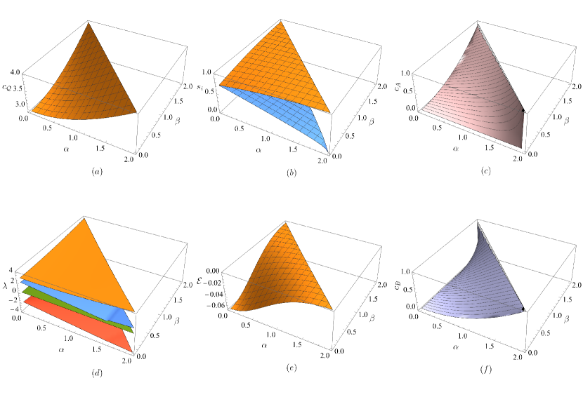
Since the largest eigenvalue of the Bell operator with the optimal measurements is non-degenerate (see FIG. 9), the maximum quantum violation $c_{\mathcal{Q}}(\alpha,\beta)$ also self-tests the state partially entangled two-qubit state $\ket{\psi}$ (the eigenvector corresponding to the largest eigenvalue). FIG. 9.b shows its Schmidt coefficients. ∎

All the results for the generalized case $\alpha\neq\beta$ are summarized in the FIG. 9.

References

- Bell [1964] J. S. Bell, On the Einstein Podolsky Rosen paradox, Physics Physique Fizika 1, 195 (1964).
- Brunner et al. [2014a] N. Brunner, D. Cavalcanti, S. Pironio, V. Scarani, and S. Wehner, Bell nonlocality, Reviews of Modern Physics 86, 419 (2014a).
- Ekert [1991] A. K. Ekert, Quantum cryptography based on Bell’s theorem, Phys. Rev. Lett. 67, 661 (1991).
- Mayers and Yao [1998] D. Mayers and A. Yao, Quantum cryptography with imperfect apparatus, in Proceedings 39th Annual Symposium on Foundations of Computer Science (IEEE, Los Alamitos, CA, 1998) p. 503.
- Barrett et al. [2005a] J. Barrett, L. Hardy, and A. Kent, No signaling and quantum key distribution, Phys. Rev. Lett. 95, 010503 (2005a).
- Acín et al. [2007] A. Acín, N. Brunner, N. Gisin, S. Massar, S. Pironio, and V. Scarani, Device-independent security of quantum cryptography against collective attacks, Phys. Rev. Lett. 98, 230501 (2007).
- Pironio et al. [2009] S. Pironio, A. Acín, N. Brunner, N. Gisin, S. Massar, and V. Scarani, Device-independent quantum key distribution secure against collective attacks, New J. Phys. 11, 045021 (2009).
- OFL [2022] Optical fiber loss and attenuation, https://www.fiberoptics4sale.com/blogs/archive-posts/95048006-optical-fiber-loss-and-attenuation (2022).
- Garg and Mermin [1987] A. Garg and N. D. Mermin, Detector inefficiencies in the Einstein-Podolsky-Rosen experiment, Phys. Rev. D 35, 3831 (1987).
- Eberhard [1993] P. H. Eberhard, Background level and counter efficiencies required for a loophole-free Einstein-Podolsky-Rosen experiment, Phys. Rev. A 47, R747 (1993).
- Massar [2002] S. Massar, Nonlocality, closing the detection loophole, and communication complexity, Phys. Rev. A 65, 032121 (2002).
- Vértesi et al. [2010] T. Vértesi, S. Pironio, and N. Brunner, Closing the detection loophole in Bell experiments using qudits, Phys. Rev. Lett. 104, 060401 (2010).
- Miklin et al. [2022] N. Miklin, A. Chaturvedi, M. Bourennane, M. Pawłowski, and A. Cabello, Exponentially decreasing critical detection efficiency for any Bell inequality, Phys. Rev. Lett. 129, 230403 (2022).
- Chaturvedi et al. [2024] A. Chaturvedi, G. Viola, and M. Pawłowski, Extending loophole-free nonlocal correlations to arbitrarily large distances, npj Quantum Information 10, 7 (2024).
- Farkas et al. [2021] M. Farkas, M. Balanzó-Juandó, K. Łukanowski, J. Kołodyński, and A. Acín, Bell nonlocality is not sufficient for the security of standard device-independent quantum key distribution protocols, Phys. Rev. Lett. 127, 050503 (2021).
- Eberhard and Rosselet [1995] P. H. Eberhard and P. Rosselet, Bell’s theorem based on a generalized EPR criterion of reality, Found. Phys. 25, 91 (1995).
- Branciard [2011] C. Branciard, Detection loophole in Bell experiments: How postselection modifies the requirements to observe nonlocality, Phys. Rev. A 83, 032123 (2011).
- Bamps and Pironio [2015] C. Bamps and S. Pironio, Sum-of-squares decompositions for a family of Clauser-Horne-Shimony-Holt-like inequalities and their application to self-testing, Phys. Rev. A 91, 052111 (2015).
- Acín et al. [2012] A. Acín, S. Massar, and S. Pironio, Randomness versus nonlocality and entanglement, Phys. Rev. Lett. 108, 100402 (2012).
- Bhatia [2013] R. Bhatia, Matrix Analysis, Graduate Texts in Mathematics (Springer New York, 2013).
- Brunner et al. [2014b] N. Brunner, D. Cavalcanti, S. Pironio, V. Scarani, and S. Wehner, Bell nonlocality, Rev. Mod. Phys. 86, 419 (2014b).
- Araújo et al. [2020] M. Araújo, F. Hirsch, and M. T. Quintino, Bell nonlocality with a single shot, Quantum 4, 353 (2020).
- Mironowicz [2023] P. Mironowicz, Semi-definite programming and quantum information, Journal of Physics A: Mathematical and Theoretical (2023).
- Gigena et al. [2022] N. Gigena, G. Scala, and A. Mandarino, Revisited aspects of the local set in CHSH Bell scenario, International Journal of Quantum Information 10.1142/s0219749923400051 (2022).
- Cabello and Larsson [2007] A. Cabello and J.-A. Larsson, Minimum detection efficiency for a loophole-free atom-photon Bell experiment, Phys. Rev. Lett. 98, 220402 (2007).
- Barrett et al. [2005b] J. Barrett, N. Linden, S. Massar, S. Pironio, S. Popescu, and D. Roberts, Nonlocal correlations as an information-theoretic resource, Phys. Rev. A 71, 022101 (2005b).
- Cope and Colbeck [2019] T. Cope and R. Colbeck, Bell inequalities from no-signaling distributions, Phys. Rev. A 100, 022114 (2019).
- Šupić and Bowles [2020a] I. Šupić and J. Bowles, Self-testing of quantum systems: a review, Quantum 4, 337 (2020a).
- Navascués et al. [2007] M. Navascués, S. Pironio, and A. Acín, Bounding the set of quantum correlations, Phys. Rev. Lett. 98, 010401 (2007).
- Garner and Araújo [2023] A. Garner and M. Araújo, Moment, https://github.com/ajpgarner/moment (2023).
- Löfberg [2004] J. Löfberg, YALMIP: a toolbox for modeling and optimization in MATLAB, in Proceedings of the CACSD Conference (Taipei, Taiwan, 2004) pp. 284–289, https://yalmip.github.io/.
- Nakata [2010] M. Nakata, A numerical evaluation of highly accurate multiple-precision arithmetic version of semidefinite programming solver: SDPA-GMP, -QD and -DD., in 2010 IEEE International Symposium on Computer-Aided Control System Design (2010) pp. 29–34, https://github.com/nakatamaho/sdpa-gmp, https://github.com/nakatamaho/sdpa-qd, https://github.com/nakatamaho/sdpa-dd.
- Masanes [2005] L. Masanes, Extremal quantum correlations for N parties with two dichotomic observables per site (2005), arXiv:quant-ph/0512100 [quant-ph] .
- Šupić and Bowles [2020b] I. Šupić and J. Bowles, Self-testing of quantum systems: a review, Quantum 4, 337 (2020b).
- Panwar et al. [2023] E. Panwar, P. Pandya, and M. Wieśniak, An elegant scheme of self-testing for multipartite Bell inequalities, npj Quantum Information 9, 71 (2023).
- Bancal et al. [2015] J.-D. Bancal, M. Navascués, V. Scarani, T. Vértesi, and T. H. Yang, Physical characterization of quantum devices from nonlocal correlations, Phys. Rev. A 91, 022115 (2015).
- Yang et al. [2014] T. H. Yang, T. Vértesi, J.-D. Bancal, V. Scarani, and M. Navascués, Robust and versatile black-box certification of quantum devices, Phys. Rev. Lett. 113, 040401 (2014).
- Lobo et al. [2024] E. P. Lobo, J. Pauwels, and S. Pironio, Certifying long-range quantum correlations through routed Bell tests, Quantum 8, 1332 (2024).
- Roy-Deloison et al. [2024] T. L. Roy-Deloison, E. P. Lobo, J. Pauwels, and S. Pironio, Device-independent quantum key distribution based on routed Bell tests (2024), arXiv:2404.01202 [quant-ph] .
- Masini et al. [2024] M. Masini, M. Ioannou, N. Brunner, S. Pironio, and P. Sekatski, Joint-measurability and quantum communication with untrusted devices (2024), arXiv:2403.14785 [quant-ph] .
- Scala et al. [2024] G. Scala, S. A. Ghoreishi, and M. Pawłowski, Advantages of quantum communication revealed by the reexamination of hyperbit theory limitations, Phys. Rev. A 109, 022230 (2024).
- Augusiak et al. [2008] R. Augusiak, M. Demianowicz, and P. Horodecki, Universal observable detecting all two-qubit entanglement and determinant-based separability tests, Phys. Rev. A 77, 030301 (2008).