Calibrated sensitivity models

Abstract

In causal inference, sensitivity models assess how unmeasured confounders could alter causal analyses. However, the sensitivity parameter in these models — which quantifies the degree of unmeasured confounding — is often difficult to interpret. For this reason, researchers will sometimes compare the magnitude of the sensitivity parameter to an estimate for measured confounding. This is known as calibration. We propose novel calibrated sensitivity models, which directly incorporate measured confounding, and bound the degree of unmeasured confounding by a multiple of measured confounding. We illustrate how to construct calibrated sensitivity models via several examples. We also demonstrate their advantages over standard sensitivity analyses and calibration; in particular, the calibrated sensitivity parameter is an intuitive unit-less ratio of unmeasured divided by measured confounding, unlike standard sensitivity parameters, and one can correctly incorporate uncertainty due to estimating measured confounding, which standard calibration methods fail to do. By incorporating uncertainty due to measured confounding, we observe that causal analyses can be less robust or more robust to unmeasured confounding than would have been shown with standard approaches. We develop efficient estimators and methods for inference for bounds on the average treatment effect with three calibrated sensitivity models, and establish that our estimators are doubly robust and attain parametric efficiency and asymptotic normality under nonparametric conditions on their nuisance function estimators. We illustrate our methods with data analyses on the effect of exposure to violence on attitudes towards peace in Darfur and the effect of mothers’ smoking on infant birthweight.

1 Introduction

In causal inference, the goal is often to estimate whether exposure to a treatment causes a change in outcomes. Randomized experiments, where exposure to treatment is randomized, are a classical method to validly estimate causal effects under minimal assumptions, but for answering many important questions they are infeasible, unethical, or too expensive. Therefore, researchers frequently estimate causal effects from observational data, where exposure to treatment is not randomized. To estimate causal effects with observational data, researchers routinely invoke the no unmeasured confounding assumption, which says that the treatment is as-if randomized within covariate strata. Unfortunately, this assumption is often implausible, because often there are variables beyond the ones observed that are associated with the treatment and outcomes of the study. Thus, it is imperative to conduct a sensitivity analysis to understand how robust causal analyses are to unmeasured confounding.

We focus on partial identification sensitivity analyses. In simplified terms, these analyses impose a bound

$$U\leq\gamma,$$ (1)

where $\gamma$ is a sensitivity parameter and $U$ is some quantification of unmeasured confounding, e.g., the difference in counterfactual regression functions (Díaz and van der Laan, 2013) or the odds ratio of the probability of treatment (Rosenbaum and Rubin, 1983; Tan, 2006). The model in (1) implies bounds on the causal effect which can be estimated from observed data. To understand the impact of unmeasured confounding, one can vary the sensitivity parameter, thereby allowing for different degrees of unmeasured confounding, and estimate bounds on and construct confidence intervals for the causal effect. Often, researchers determine the value of $\gamma$ where the confidence interval includes zero, because it indicates the level of unmeasured confounding where the causal effect estimate is non-significant. If the resulting $\gamma$ value is large, causal analyses are said to be robust to unmeasured confounding; conversely, if the $\gamma$ value is small, analyses are said to be sensitive to unmeasured confounding.

However, it can be difficult to gain intuition for the absolute size of the sensitivity parameter $\gamma$. Therefore, recent research has proposed calibrating (or, benchmarking) results by estimating measured confounding (e.g., Zhang and Zhao (2022); Cinelli and Hazlett (2020); Chernozhukov et al. (2022); Veitch and Zaveri (2020); Bonvini et al. (2022); Rubinstein et al. (2022); Huang and Pimentel (2022); Franks et al. (2020); Hsu and Small (2013); Lu and Ding (2023)). For example, it is common to leave out one variable at a time, re-estimate the causal effect, and define measured confounding as the largest difference in estimated effects. Customarily, one can then decide whether the causal effect estimate is robust to unmeasured confounding by comparing the sensitivity parameter to estimated measured confounding. For example, one might compare the level of the sensitivity parameter where confidence intervals for the causal effect include zero to the estimated measured confounding. If the measured confounding were much smaller, this might be evidence that the causal effect estimate is robust to unmeasured confounding, because unmeasured confounders would need to have a larger impact on the causal effect than measured confounders to potentially reverse conclusions from the causal analysis.

This approach, which we refer to as “post hoc calibration”, suffers from two drawbacks. First, uncertainty in the estimate for measured confounding is unaccounted for. As we demonstrate, correctly accounting for this uncertainty can yield different conclusions for how robust the causal effect is to unmeasured confounding — both more and less robust are possible. Second, researchers rarely justify their choice of measured confounding. Therefore, the trade-offs associated with a particular choice of measured confounding are unclear. The choice of measured confounding is important, because it affects how one interprets the robustness of causal analyses.

The lack of interpretability of the sensitivity parameter $\gamma$ and the deficiencies of post hoc calibration motivate our novel approach, the calibrated sensitivity model. In simplified terms, calibrated sensitivity models use sensitivity models as a building block to impose a bound

$$U\leq\Gamma M,$$ (2)

where $U$ is unmeasured confounding, $M$ is measured confounding, and $\Gamma$ is a sensitivity parameter. In other words, calibrated sensitivity models bound the degree of unmeasured confounding by a multiple of measured confounding. As we demonstrate, a calibrated sensitivity analysis can be conducted like a standard sensitivity analysis, but in a way that naturally incorporates estimation and uncertainty quantification for measured confounding. Furthermore, there is no need for post hoc calibration, because the sensitivity parameter is immediately interpretable as a unit-less bound on the ratio of unmeasured confounding divided by measured confounding.

1.1 Our contributions

The goal of this manuscript is to define calibrated sensitivity models, illustrate their benefits, and demonstrate how to conduct estimation and inference with them. To that end, our primary contributions are:

1. We formally define several calibrated sensitivity models. These are based on popular sensitivity models defined on the outcome regression function and propensity score (Luedtke et al., 2015; Yadlowsky et al., 2022; Rosenbaum, 2002). We consider multiple definitions of measured confounding and discuss how one might justify each.

2. We establish methods for estimation and inference with calibrated sensitivity models which account for uncertainty in estimating measured confounding.

3. We provide several data analyses, which demonstrate how to analyze data with a calibrated sensitivity model, and highlight the differences between our novel methods and standard approaches.

1.2 Structure of the paper

In Section 1.3, we define notation. In Section 1.4, we provide a motivating illustration showing the advantages of calibrated sensitivity models. In Section 2, we outline the data generating process and review the Average Treatment Effect (ATE) and the assumptions required to identify it, sensitivity analyses and post-hoc calibration, and different quantifications of measured confounding and their strengths and weaknesses. In Section 3, we introduce calibrated sensitivity models and provide three examples. In Section 4, we identify bounds on the ATE under the three example models. In Section 5, we demonstrate methods for estimation and inference for bounds on the ATE. In Section 6, we illustrate our methods with real data analyses on the effect of exposure to violence on attitudes towards peace in Darfur and the effect of mothers’ smoking on infant birth weight. Finally, in Section 7, we conclude and discuss.

1.3 Notation

We use $\mathbb{E}$ for expectation, $\mathbb{V}$ for variance, and $\mathbb{P}$ for probability. We use $\mathbb{P}_{n}\{f(Z)\}=\frac{1}{n}\sum_{i=1}^{n}f(Z_{i})$ as shorthand for the sample average of $f(X)$. When $x\in\mathbb{R}^{d}$ we let $\lVert x\rVert^{2}=\sum_{j=1}^{d}x_{j}^{2}$, and for generic possibly random functions $f$ we let $\lVert f(Z)\rVert_{p}^{p}=\int_{\mathcal{Z}}f(z)^{p}d\mathbb{P}(z)$ denote the $L_{p}^{p}(\mathbb{P})$ norm for $1\leq p<\infty$ and $\lVert f(Z)\rVert_{\infty}=\sup_{x\in\mathcal{X}}|f(x)|$. We use $\rightsquigarrow$ to denote convergence in distribution and $\stackrel{{\scriptstyle p}}{{\rightarrow}}$ for convergence in probability. Finally, for a positive integer $d$ we use the notation $[d]=\{1,\dots,d\}$.

1.4 Motivating illustration and advantages of calibrated sensitivity models

Suppose $\psi_{\ast}$ is a causal effect and $\psi$ is an observed data analog depending on $d$ measured confounders. For example, $\psi_{\ast}$ could be the ATE, i.e., $\psi_{\ast}=\mathbb{E}(Y^{1}-Y^{0})$ where $Y^{a}$ is the potential outcome under treatment $a$, while $\psi$ is the adjusted mean difference with all covariates, i.e., $\psi=\mathbb{E}\{\mathbb{E}(Y\mid A=1,X)-\mathbb{E}(Y\mid A=0,X)\}$. Further suppose that if there were no unmeasured confounders then $\psi_{\ast}=\psi$ and otherwise $\psi_{\ast}\neq\psi$. Consider a simple sensitivity model, which imposes a bound at the level of the causal effect (Luedtke et al., 2015),

$$\left|\psi_{\ast}-\psi\right|\leq\gamma.$$ (3)

This model illustrates the first issue common to many sensitivity models — it is difficult to interpret levels of $\gamma$. Indeed, with this particular model, interpretability is a critical issue, as it may be un-intuitive to bound the error due to unmeasured confounding at the level of the effect itself. While this issue may be less severe with other popular models defined at the level of the outcome regression or propensity score, it exists nonetheless.

The lack of interpretability of the sensitivity parameter has inspired post hoc calibration, where one estimates measured confounding analogous to unmeasured confounding. In our running example, one could consider maximum change in the adjusted mean difference from leaving out one covariate at a time (we review different options in Section 2.4),

$$M=\max_{j\in[d]}\left|\psi-\psi_{-j}\right|,$$ (4)

where $\psi_{-j}=\mathbb{E}\{\mathbb{E}(Y\mid A=1,X_{-j})-\mathbb{E}(Y\mid A=0,X_{-j})\}$ and $X_{-j}$ excludes the $j^{th}$ covariate. Customarily, researchers then interpret levels of $\gamma$ by comparing it to $\widehat{M}$, an estimate of $M$.

Figure 1(a) illustrates results from a data analysis using the model in (3). The x-axis is the sensitivity parameter $\gamma$ and the y-axis is on the scale of the ATE. The ATE estimate is the horizontal dashed black line, estimates for the bounds are in purple, and 95% confidence intervals for the ATE are in blue. Meanwhile, the estimate of measured confounding, $\widehat{M}=\max_{j\in[d]}|\widehat{\psi}-\widehat{\psi}_{-j}|\approx 46.6$, is shown as the vertical dashed blue line. While Figure 1(a) allows easier interpretation of levels of $\gamma$, it also clarifies a crucial deficiency with post hoc calibration: uncertainty in the estimated measured confounding $\widehat{M}$ is unaccounted for. As a result, when researchers decide whether their effect is robust to unmeasured confounding by comparing $\gamma$ with $\widehat{M}$, their conclusions may be incorrect.

In this paper, we propose novel calibrated sensitivity models to address the lack of interpretability of the sensitivity parameter $\gamma$ and allow for uncertainty quantification that accounts for uncertainty in estimated measured confounding. For our running example, based on the analysis above, a calibrated sensitivity model would be to bound the error due to unmeasured confounding by a multiple of the maximum change in the adjusted mean difference from leaving out one covariate at a time:

$$\left|\psi_{\ast}-\psi\right|\leq\Gamma\max_{j\in[d]}\left|\psi-\psi_{-j}\right|.$$ (5)

Equation (5) immediately demonstrates how a calibrated sensitivity model can be more intuitive than the related sensitivity model. In the sensitivity model in (3), it is difficult to interpret different levels of $\gamma$, which is the motivation for post hoc calibration. By contrast, with the calibrated sensitivity model, $\Gamma$ is already calibrated — it is a unit-less bound on the ratio of unmeasured divided by measured confounding. This can be easier to reason about. Indeed, previous work has emphasized the desirability of unit-less sensitivity parameters (Veitch and Zaveri, 2020; Imbens, 2003; Bonvini and Kennedy, 2022); however, previously considered parameters were not explicitly calibrated to measured confounding, unlike $\Gamma$ in (5).

Moreover, with calibrated sensitivity models, confidence intervals for the causal effect that account for the uncertainty in estimated measured confounding can be constructed. In this paper, we develop methods to do so. While this is possible with sensitivity models and post hoc calibration, it has not previously been considered in the literature, and it is simpler with calibrated sensitivity models.

Figure 1 illustrates how results could differ when uncertainty in estimating measured confounding is accounted for. Figure 1(b) shows the results from the same data analysis as before but using the calibrated sensitivity model in (5) and accounting for uncertainty in $\widehat{M}$. The estimated bounds are in purple and the confidence band is in red. The red confidence bands from the calibrated sensitivity analysis can be wider than the blue confidence bands from the standard sensitivity analysis (e.g., when $\Gamma>2$, $\gamma>100$), as one might intuitively expect, but can also provide tighter confidence intervals (e.g., the upper limit of the confidence band when $\Gamma<2$, $\gamma<100$). Since the confidence intervals can be narrower or wider, calibrated sensitivity models can illuminate that results may be more robust or less robust than previously thought, after accounting for uncertainty in estimating measured confounding. Whether the calibrated confidence intervals are narrower or wider depends on the covariance between the estimators for the bounds and the estimator for measured confounding. We provide a simplified analysis in Section 5.5 to build intuition for when the calibrated confidence intervals will be narrower or wider.

Remark 1.

The estimated bounds are the same in both analyses up to a standardization of the x-axis. We give further details as to why this occurs in Section 4.1, but in short, for the sensitivity model in (3) one can standardize the x-axis by measured confounding — i.e., change the x-axis to $\gamma/\widehat{M}$ — to point estimate the same bounds as the calibrated sensitivity analysis using the model in (5).

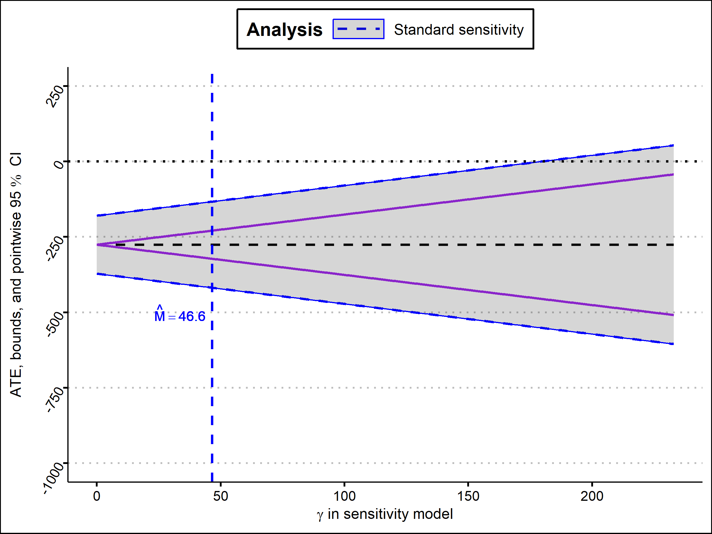
(a) Sensitivity analysis with post hoc calibration

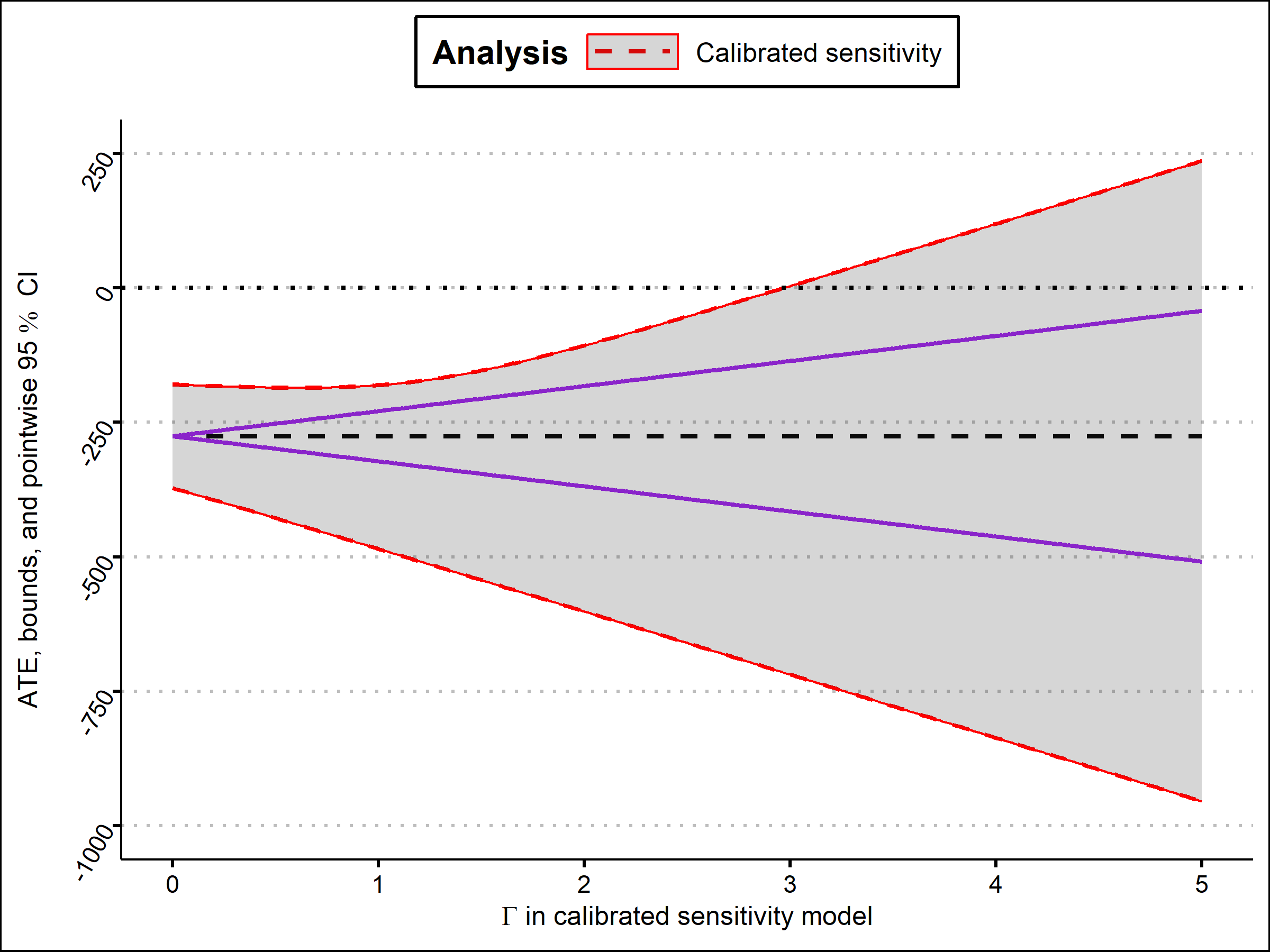
(b) Calibrated sensitivity analysis

Figure 1: Example sensitivity and calibrated sensitivity analyses. Bounds (purple) on the ATE (y-axis) are shown at different levels of unmeasured confounding (x-axis). The left panel shows the confidence band (blue) without accounting for uncertainty in estimating measured confounding, while the right panel displays the confidence band (red) that incorporates uncertainty in estimating measured confounding.

Calibrated sensitivity models offer two further potential benefits. First, they can be constructed with less popular but perhaps more useful quantifications of unmeasured confounding, which might increase the adoption of sensitivity analyses in practice. For instance, the model in our running example (in (3)), which bounds unmeasured confounding at the level of the causal effect, is not widely used for standard sensitivity analyses, presumably due to the interpretability issues discussed above. However, within a calibrated sensitivity model (e.g., in (5)), it is more interpretable, and it could offer advantages over standard quantifications of unmeasured confounding. Indeed, the model in (5) could be useful to practitioners because of its flexibility, as it can be applied to sensitivity analyses with any causal effect identified under unmeasured confounding or could be used to assess violations of other identifying assumptions. By contrast, many popular quantifications of unmeasured confounding are not so flexible; for example, models defined on the odds ratio of propensity scores do not easily generalize beyond binary treatment (Rosenbaum, 2002; Tan, 2006). Other quantifications of unmeasured confounding, such as distributional distances or average strengths of unmeasured confounding (Luedtke et al., 2015; Zhang and Zhao, 2022; Jin et al., 2022), can also be interpretable within a calibrated sensitivity framework, and may offer advantages over quantifications of unmeasured confounding which are currently more popular.

Finally, incorporating measured confounding as an explicit assumption in a calibrated sensitivity model can encourage researchers to better justify their choice of measured confounding. In many post hoc calibration analyses, the choice of measured confounding is not well-justified (with notable exceptions; e.g., Veitch and Zaveri (2020); Franks et al. (2020); Cinelli and Hazlett (2020), among others), perhaps because it is not immediately apparent that it is a model assumption. By contrast, when measured confounding is incorporated into the calibrated sensitivity model at the start of the analysis, rather than afterwards, it is clearer that researchers must assume and justify whatever quantification of measured confounding they use. For example, in (5), it is evident that one should justify the choice of maximum leave-one-out measured confounding. We discuss the strengths and weaknesses of this and other definitions of measured confounding in Section 2.4.

In summary, calibrated sensitivity models offer at least four advantages over standard sensitivity models:

1. Unlike the sensitivity parameter $\gamma$, which researchers often struggle to interpret, the calibrated sensitivity parameter $\Gamma$ is calibrated by construction and is an intuitive, unit-less bound on the ratio of unmeasured to measured confounding.

2. Confidence intervals accounting for uncertainty in estimated measured confounding can be constructed.

3. New quantifications of unmeasured confounding, which may have advantages over standard methods (e.g., more flexible, simpler), can be bounded in an intuitive manner. The resulting calibrated sensitivity models may be more useful tools to practitioners, potentially increasing the adoption of sensitivity analyses in practice.

4. Explicitly incorporating measured confounding as an assumption in a calibrated sensitivity model can encourage researchers to better justify their choice of measured confounding.

2 Setup and background

In this section, we describe the data generating process, causal assumptions, and the ATE. We then review the sensitivity analysis literature, and conclude with a review of different quantifications of measured confounding.

2.1 Data and assumptions

We assume we observe $n$ observations $\{Z_{i}\}_{i=1}^{n}\stackrel{{\scriptstyle iid}}{{\sim}}\mathcal{P}$ where $Z$ is a tuple $(X,A,Y)$, $X\in\mathbb{R}^{d}$ are $d$-dimensional covariates, $A\in\{0,1\}$ is a binary exposure, and $Y\in\mathbb{R}$ is an outcome. We use subscript notation to develop calibrated sensitivity models: $X_{-j}$ excludes the $j^{th}$ covariate, $X_{j}$ is the $j^{th}$ covariate, and, for any set $S\subseteq[d]$, $X_{-S}$ excludes the covariates corresponding to $S$. We let $Z_{-S}=\{X_{-S},A,Y\}$ and assume $\{Z_{-S}\}_{i=1}^{n}\stackrel{{\scriptstyle iid}}{{\sim}}\mathcal{P}_{-S}$, i.e., the data with only covariates $X_{-S}$ is drawn from some distribution $\mathcal{P}_{-S}$. Additionally, we denote unmeasured confounders by $W$ and define potential outcomes $Y^{a}$ as the outcome that would have been observed under exposure $A=a$. Finally, we will refer to $\pi_{a}(X)=\mathbb{P}(A=a\mid X)$ as the “propensity score” and $\mu_{a}(X)=\mathbb{E}(Y\mid A=a,X)$ as the “outcome regression function”, and generically we will refer to them as “nuisance functions”. Other nuisance functions will be defined when they appear.

We make two standard causal assumptions.

Assumption 1.

Consistency: $A=a\implies Y=Y^{a}$.

Assumption 2.

Positivity: $\exists\ \varepsilon>0$ such that $\mathbb{P}\left\{\varepsilon\leq\pi_{1}(X)\leq 1-\varepsilon\right\}=1$.

Consistency says that we observe the potential outcome relevant to the observed exposure. It would be violated if, for example, there were interference between subjects such that one subject’s treatment affected another’s outcome. Positivity says that all subjects have a non-zero probability of exposure. The literature addressing violations of each of these assumptions is too large to summarize here, but see, for example, Tchetgen and VanderWeele (2012) and Westreich and Cole (2010) for discussion of violations of consistency and positivity, respectively.

2.2 The Average Treatment Effect

While some of our methods generalize to other causal estimands, for simplicity we focus on the ATE:

$$\psi_{\ast}=\mathbb{E}(Y^{1}-Y^{0}).$$ (6)

The ATE is a canonical causal effect. It is the mean difference in potential outcomes if everyone were exposed to some variable of interest versus if no one were exposed. If, in addition to consistency and positivity, one were to assume no unmeasured confounding holds with the observed covariates — i.e., that $(Y^{0},Y^{1})\mathchoice{\mathrel{\hbox to0.0pt{$\displaystyle\perp$\hss}\mkern 4.0mu{\displaystyle\perp}}}{\mathrel{\hbox to0.0pt{$\textstyle\perp$\hss}\mkern 4.0mu{\textstyle\perp}}}{\mathrel{\hbox to0.0pt{$\scriptstyle\perp$\hss}\mkern 4.0mu{\scriptstyle\perp}}}{\mathrel{\hbox to0.0pt{$\scriptscriptstyle\perp$\hss}\mkern 4.0mu{\scriptscriptstyle\perp}}}A\mid X$ — then the ATE could be identified, in the sense that it could be written in terms of fully observed quantities. Specifically, the ATE can be identified by the mean difference in outcome regression functions under exposure and control:

$$\psi=\mathbb{E}\{\mu_{1}(X)-\mu_{0}(X)\}.$$ (7)

We will refer to $\psi$ as an “adjusted mean difference” to differentiate it from the causal ATE in (6). We define the adjusted mean difference with a general covariate set $X_{-S}$ as

$$\psi_{-S}=\mathbb{E}\{\mu_{1}(X_{-S})-\mu_{0}(X_{-S})\}.$$ (8)

Without no unmeasured confounding or an alternative assumption (e.g., that an instrumental variable or regression discontinuity exists), one cannot identify $\psi_{\ast}$ such that $\psi_{\ast}=\psi$. To address this, there is a large literature on sensitivity analyses, which impose an assumption on the effect of unmeasured confounding.

2.3 Sensitivity analyses

Here, we briefly review the large literature on sensitivity analyses, which dates back at least to the seminal analysis of the effect of smoking on lung cancer incidence in Cornfield et al. (1959). Recent reviews on sensitivity analyses are Liu et al. (2013) and Richardson et al. (2014). Modern sensitivity models could arguably be split into two types:

1. Models which admit point identification of the causal effect, and

2. Models which admit partial (or, set) identification of the causal effect.

Generally, point identification models impose a specific form on the relationship between the unmeasured confounder and the observed data. For example, Scharfstein et al. (2021) consider a model of the form

$$p(Y^{a}=y\mid A=1-a,X=x)=p(Y^{a}=y\mid A=a,X=x)q_{a}(Y^{a}=y,X=x;\gamma),$$ (9)

where $p$ is the density of $Y^{a}$ and $q_{a}(Y^{a}=y,X=x;\gamma)$ is a researcher-specified transformation which depends on the sensitivity parameter $\gamma$ and relates the unidentified potential outcome density on the left-hand side of (9) to the identified density on the right-hand side of (9). There are many popular models in the literature (e.g., Carnegie et al. (2016); Imbens (2003); Robins (1999); Brumback et al. (2004); Robins et al. (2000); Franks et al. (2020); Scharfstein et al. (2021); Veitch and Zaveri (2020); VanderWeele and Arah (2011); Zhang and Tchetgen Tchetgen (2022), among others). Under such an assumption, the ATE (for example) can be identified and estimated, and typically researchers examine how the ATE changes with different values of the sensitivity parameter $\gamma$. We direct interested readers to the literature reviews mentioned earlier, along with Section 2.2 of Scharfstein et al. (2021).

Partial identification sensitivity analysis, which we focus on in this paper, is the other important type of sensitivity analysis. Generally, a partial identification sensitivity analysis comprises the following steps:

1. The researcher chooses a quantification of unmeasured confounding, $U$, and imposes a bound $U\leq\gamma$, where $\gamma\in\mathbb{R}^{+}$ is the sensitivity parameter (we summarize choices of $U$ below).

2. (Partial identification) The bound in step 1 implies bounds on the causal effect. We denote the lower and upper bounds on the ATE as $\ell:\mathcal{P}\times\mathbb{R}^{+}\to\mathbb{R}$ and $u:\mathcal{P}\times\mathbb{R}^{+}\to\mathbb{R}$, respectively, so that

   $$\psi_{\ast}\in\left[\ell(\gamma),u(\gamma)\right].$$ (10)

   The bounds depend on the observed data and the sensitivity parameter.

3. For various levels of $\gamma$, the researcher estimates the bounds and constructs confidence intervals for the bounds and, by extension, the causal effect (see, e.g., the results in Figure 1(a)).

4. (Post hoc calibration) To interpret levels of $\gamma$, the researcher estimates a quantification of measured confounding $M$ (we discuss choices below). Generally, $M$ is a measured quantity analogous to $U$. Often, $M$ is estimated by leaving out one or several variables at a time and estimating measured confounding implied by those variables. Finally, the researcher compares the level of $\gamma$ from step 3. to the estimate $\widehat{M}$.

As far as we are aware, these four steps constitute a comprehensive sensitivity analysis in the current state of the literature, though step 4 is not always performed. In step 3, researchers might examine other statistics, such as the level of $\gamma$ where confidence intervals for the causal effect include zero, i.e., where a significant effect estimate is nullified, and compare this to the level of measured confounding in post hoc calibration.

Within partial identification sensitivity analyses, the key choices are the quantifications of unmeasured confounding $U$ and measured confounding $M$. Here, we review choices of unmeasured confounding and the next section provides examples of measured confounding.

Early partial identification models imposed bounds which follow directly from bounds on the data itself (Manski, 1990; Robins, 1989), e.g., if the outcome is bounded this implies a bound on the ATE. More recent work has bounded the error due to unmeasured confounding at the level of the causal effect itself (Luedtke et al., 2015), the odds ratio of the propensity score (Rosenbaum, 2002; Soriano et al., 2023; Tan, 2006; Zhao et al., 2019; Yadlowsky et al., 2022; Zhang and Zhao, 2022; Dorn and Guo, 2023; Dorn et al., 2024), the direct change in the propensity score (Masten and Poirier, 2018; Masten et al., 2023), the change in or ratio of outcome regression functions (Díaz and van der Laan, 2013; Luedtke et al., 2015; van der Laan et al., 2018; Lu and Ding, 2023), the change in explained variance of the outcome regressions or the propensity score (Chernozhukov et al., 2022; Cinelli and Hazlett, 2020; Huang and Pimentel, 2022), and the proportion of units confounded (Bonvini and Kennedy, 2022). There are others, and we summarize a non-exhaustive snapshot of the literature in Table 1.

Remark 2.

An often over-looked model choice when quantifying unmeasured confounding is the choice of distance, e.g., $L_{p}(\mathbb{P})$ norm. Most models are defined in terms of $L_{\infty}$ norm and bound maximum unmeasured confounding. However, more recent work has considered $L_{p}$ norms for $p<\infty$ and bounded average unmeasured confounding (e.g., Zhang and Zhao (2022)). We consider both $p=\infty$ and $p=2$ in our examples in Section 3. In Section 1.4, we discussed the advantages of considering average unmeasured confounding within a calibrated sensitivity model; in particular, one can benefit from any advantages that arise from bounding average unmeasured confounding instead of maximum unmeasured confounding, but still have intuition for the size of the calibrated sensitivity parameter because it is calibrated by construction.

With a specific choice of $U$ in Table 1, there are many methods for conducting steps 1-3 and estimating bounds on the ATE. In the next section, we review choices of measured confounding which researchers have used to calibrate $\gamma$ in step 4.

Sensitivity Model	Quantification of unmeasured confounding $U$	Examples
Effect Differences	$\left|\psi_{\ast}-\psi\right|$	Luedtke et al. (2015)
Potential Outcome Regression Differences	$\Big{\lVert}\mathbb{E}(Y^{a}\mid A=a,X)-\mathbb{E}(Y^{a}\mid A=1-a,X)\Big{\rVert}_{p}$	Díaz and van der Laan (2013) Luedtke et al. (2015)
Potential Outcome Regression Ratios	$\left\lVert\frac{\mathbb{E}(Y^{a}\mid A=1-a,X)}{\mathbb{E}(Y^{a}\mid A=a,X)}\right\rVert_{p}$	Luedtke et al. (2015); Lu and Ding (2023)
Direct Propensity Score Differences	$\left\lVert\pi_{1}(X)-\pi_{1}(X,W)\right\rVert_{\infty}$	Masten and Poirier (2018)
Propensity Score Odds Ratios	$\left\lVert\frac{\text{odds}\left\{\pi_{1}(X)\right\}}{\text{odds}\left\{\pi_{1}(X,W)\right\}}\right\rVert_{p}$ or $\left\lVert\frac{\text{odds}\left\{\pi_{1}(X,\widetilde{W})\right\}}{\text{odds}\left\{\pi_{1}(X,W)\right\}}\right\rVert_{p}$	Rosenbaum (2002); Tan (2006)
Explained Variance	$\frac{\lVert\mu_{A}(X,W)-\mu_{A}(X)\rVert_{2}^{2}}{\lVert Y-\mu_{A}(X)\rVert_{2}^{2}}$ and $\frac{\mathbb{E}\left(\big{\{}\pi_{1}(X,W)\pi_{0}(X,W)\big{\}}^{-1}\right)}{\mathbb{E}\left(\big{\{}\pi_{1}(X)\pi_{0}(X)\big{\}}^{-1}\right)}$	Chernozhukov et al. (2022) — assuming $\psi_{\ast}=\mathbb{E}(Y^{1}-Y^{0})$ (see Remark 3) Cinelli and Hazlett (2020)
Explained Variance	$\left\lVert\frac{\mathbb{V}\left[\text{odds}\{\pi_{1}(X,W))\}\right]}{\mathbb{V}\left[\text{odds}\{\pi_{1}(X)\}\right]}\right\rVert_{\infty}$	Huang and Pimentel (2022)

Table 1: Partial identification sensitivity models. This table describes several sensitivity models that bound a quantification of unmeasured confounding and allow for partial identification of the ATE.

2.4 Measured confounding

For both point identification and partial identification sensitivity analyses, researchers have considered calibrating their sensitivity parameters to the observed data by estimating measured confounding (Bonvini et al., 2022; Franks et al., 2020; Rubinstein et al., 2022; Cinelli and Hazlett, 2020; Veitch and Zaveri, 2020; Zhang and Zhao, 2022; Hsu and Small, 2013; Zhang and Small, 2020; Lu and Ding, 2023), and multiple authors have observed that different quantifications of measured confounding have advantages and disadvantages (e.g., (Cinelli and Hazlett, 2020) Section 4, Veitch and Zaveri (2020) Section 3). In general, there are three choices when constructing measured confounding $M$:

1. the quantification of measured confounding (e.g., effect difference, change in outcome regressions, etc.),

2. what covariate subsets are omitted, and

3. how sub-quantifications of measured confounding across covariate subsets are aggregated.

For the quantification of measured confounding in 1., the simplest choice is the notion of measured confounding that is analogous to unmeasured confounding. For example, if $U=|\psi_{\ast}-\psi|$, then measured confounding would be $|\psi-\psi_{-S}|$ for different sets $S$. However, when the analogous notion of measured confounding is difficult to estimate researchers may prefer to consider a smooth approximation of it. For example, when unmeasured confounding is an $L_{\infty}$ norm, researchers might prefer to define measured confounding as a smooth approximation of it, because $L_{\infty}$ norms cannot be estimated at $\sqrt{n}$ rates under nonparametric assumptions (Lepski et al., 1999).

To illuminate the second and third choices for measured confounding, we quantify unmeasured and measured confounding at the level of the causal effect, such that $U=|\psi_{\ast}-\psi|$ and $M$ is defined in terms of the difference between $\psi$ and $\psi_{-S}$ for different sets $S$. In Section 3, we demonstrate how the second and third choices discussed here generalize to other quantifications of unmeasured and measured confounding.

The second choice in measured confounding is which subsets are considered. The leave-one-out (LOO) error, which considers measured confounding from leaving out one variable at a time, is a natural starting point. Mathematically, the LOO error for the $j^{th}$ covariate is $\left|\psi-\psi_{-j}\right|$, where $\psi_{-j}$ is the functional with variable $X_{j}$ excluded (e.g., when $\psi$ is the adjusted mean difference, then $\psi_{-j}=\mathbb{E}\{\mu_{1}(X_{-j})-\mu_{0}(X_{-j})\}$). The LOO error is a well-understood measure of variable importance (Lei et al., 2018), and it is computationally tractable, requiring only on the order of $d$ estimators to estimate all leave-one-out errors. However, as was observed in Cinelli and Hazlett (2020) and Veitch and Zaveri (2020), an important disadvantage is that it might be misleading if several variables are similar. Leaving out one variable at a time will not capture the joint effects of several similar variables, and their joint effect may be a better proxy for the effect of an unmeasured confounder than any individual effect.

When several variables are similar, a researcher could start with the leave-one-out error and then also leave out others groups of variables, which we refer to as the leave-some-out (LSO) error. For example, if $S$ is an index referring to some set of covariates (e.g., $S=\{1,2\}$), then the $S$-LSO error is $\left|\psi-\psi_{-S}\right|$, where $\psi_{-S}$ is the causal effect with the covariates referred to in $S$ removed. The leave-some-out error can capture the joint effect of several correlated variables that would be missed in the leave-one-out error. However, it also requires researchers to decide which subsets of covariates to leave out. This may be difficult. An extreme solution to this problem is the leave-every-out error, which leaves out every possible subset of covariates. This model is computationally intensive since it requires on the order of $2^{d}$ estimators. Some analyses have also considered leaving out all the covariates or a random half of the covariates (Bonvini et al., 2022; Rubinstein et al., 2022).

The third choice is how to aggregate sub-quantifications of measured confounding across the subsets considered. Maximums and averages are natural options. For example, the maximum leave-one-out error is $\max_{j\in[d]}\left|\psi-\psi_{-j}\right|$ while the average leave-one-out error is $\frac{1}{d}\sum_{j=1}^{d}\left|\psi-\psi_{-j}\right|$. Either could be advantageous. Because averages are no larger than maximums, the average error provides tighter bounds than the maximum, which may be appropriate.

Remark 3.

Here, we have only summarized previously considered notions of measured confounding, and considering other metrics would be an interesting avenue of future work. Because measured confounding is a notion of variable importance, one might also consider other approaches from the wider variable importance literature. For example, Shapley values are a popular measure of variable importance in machine learning, and may be useful for understanding measured confounding (Shapley, 1953; Williamson et al., 2021; Rozemberczki et al., 2022).

3 Calibrated sensitivity analyses and three example models

In this section, we outline the generic steps of partial identification calibrated sensitivity analysis, highlighting where they differ from partial identification sensitivity analyses reviewed in Section 2.3, and construct three example calibrated sensitivity models.

3.1 Calibrated sensitivity analyses

Calibrated sensitivity analyses comprise the following steps:

1. The researcher chooses a quantification of unmeasured confounding $U$ and a quantification of measured confounding $M$, and imposes a bound $U\leq\Gamma M$ where $\Gamma\in\mathbb{R}^{+}$ is the sensitivity parameter. This differs from a sensitivity analysis because the model includes measured confounding.

2. (Partial identification) The bound in step 1. implies bounds on the causal effect. We denote lower and upper bounds on the ATE as $\mathcal{L}:\mathcal{P}\times\mathbb{R}^{+}\to\mathbb{R}$ And $\mathcal{U}:\mathcal{P}\times\mathbb{R}^{+}\to\mathbb{R}$, respectively, so that

   $$\psi_{\ast}\in\left[\mathcal{L}(\Gamma),\ \mathcal{U}(\Gamma)\right].$$ (11)

   The bounds depend on the observed data and the sensitivity parameter. This differs from a sensitivity analysis because $\mathcal{L}$ and $\mathcal{U}$ are different functionals from $\ell$ and $u$ in (10) — $\mathcal{L}$ and $\mathcal{U}$ depend on measured confounding.

3. For various levels of $\Gamma$, the researcher estimates the bounds and constructs confidence intervals for the bounds and, by extension, the causal effect (see, e.g., Figure 1(b)). Unlike with standard sensitivity analyses, the method for constructing confidence intervals accounts for uncertainty in estimating measured confounding.

These three steps constitute a comprehensive calibrated sensitivity analysis. Unlike with standard sensitivity analyses, a final post hoc calibration step is not necessary, because $\Gamma$ is already calibrated by construction.

3.2 Three example calibrated sensitivity models

Here, we give three example models which illustrate particular choices of unmeasured confounding $U$ and measured confounding $M$ in the bound $U\leq\Gamma M$. We use these examples to identify and estimate bounds on the ATE in Sections 4 and 5. The first model is the maximum leave-one-out effect differences model (which we also refer to as the “effect differences model”).

Calibrated sensitivity model 1.

(Maximum leave-one-out effect differences)

$$\left|\psi_{\ast}-\psi\right|\leq\Gamma\max_{j\in[d]}\left|\psi-\psi_{-j}\right|,$$ (12)

where $\Gamma\in(0,\infty)$ is the sensitivity parameter, $\psi$ is the adjusted mean difference in (8) with $X$ covariates (i.e., all covariates) and $\psi_{-j}$ is the adjusted mean difference with $X_{-j}$ covariates (i.e., without covariate $X_{j}$).

The maximum LOO effect differences model uses the maximum leave-one-out error and quantifies unmeasured and measured confounding at the level of the causal effect. This quantification of unmeasured confounding was considered in Luedtke et al. (2015) (and in Section 1.4). While quantifying confounding at the level of the causal effect is less popular than the other approaches we consider in the next two examples, we include this approach because the resulting analysis is intuitive and simple, and therefore eases exposition of the main ideas in this paper. Furthermore, this choice of $U$ and $M$ has other benefits when considered within a calibrated sensitivity model. This model generalizes to any causal effect which is identifiable under no unmeasured confounding. Moreover, estimation is straightforward, and does not require the derivation of new estimators; instead, one can re-run an estimator for $\psi$, but with fewer covariates included.

The second model is the maximum leave-one-out $L_{\infty}$ propensity score odds ratio model (which we also refer to as the “odds ratio model”).

Calibrated sensitivity model 2.

(Maximum leave-one-out $L_{\infty}$ propensity score odds ratio)

$$\sup_{x,w,\widetilde{w}}\left|\log\left[\frac{\text{odds}\{\pi_{1}(x,w)\}}{\text{odds}\{\pi_{1}(x,\widetilde{w})\}}\right]\right|\leq\Gamma\max_{j\in[d]}\sup_{x_{-j},x_{j},\widetilde{x}_{j}}\left|\log\left[\frac{\text{odds}\{\pi_{1}(x_{-j},x_{j})\}}{\text{odds}\{\pi_{1}(x_{-j},\widetilde{x}_{j})\}}\right]\right|$$ (13)

where $\Gamma\in(0,\infty)$ is the sensitivity parameter, $\pi_{1}$ is the propensity score, and $\text{odds}(p)=p/(1-p)$.

The maximum LOO odds ratio model uses the maximum leave-one-out error again and a popular quantification of unmeasured confounding — the maximum propensity score odds ratio induced by the unmeasured confounder (Rosenbaum and Rubin, 1983; Yadlowsky et al., 2022). We state the model in terms of the log-odds ratio so that the constraint is additive rather than multiplicative and the sensitivity parameter $\Gamma$ takes the same range and has the same meaning as in the other two models.

In the odds ratio model, the unmeasured and measured confounding are defined in terms of a supremum, which is a popular definition in the literature. A drawback of this is that it is necessary to estimate the supremum, and $\sqrt{n}$-estimation is not possible under nonparametric assumptions (Lepski et al., 1999). Therefore, in Section 5, we will consider the projection of measured confounding onto a finite-dimensional model, for which one can construct $\sqrt{n}$-efficient estimators and methods for inference.

The third model is the average leave-some-out $L_{2}$ outcome regression differences model (which we also refer to as the “outcome model”).

Calibrated sensitivity model 3.

(Average leave-some-out $L_{2}$ outcome regression differences)
 For $a\in\{0,1\}$,

$$\left\lVert\mathbb{E}(Y^{a}\mid A=a,X)-\mathbb{E}(Y^{a}\mid A=1-a,X)\right\rVert_{2}^{2}$$

$$\hskip 72.26999pt\leq\frac{\Gamma}{|\mathcal{S}|}\sum_{S\in\mathcal{S}}\left\lVert\mu_{a}(X_{-S})-\mathbb{E}\big{\{}\mu_{a}(X)\mid A=1-a,X_{-S}\big{\}}\right\rVert_{2}^{2},$$ (14)

where $\Gamma\in(0,\infty)$ is the sensitivity parameter and $\mathcal{S}$ is a set of subsets of $[d]$.

The average LSO outcome model is also based on a popular quantification of unmeasured confounding — the difference between the potential outcome regressions under the observed treatment and the opposite treatment (Díaz and van der Laan, 2013; Luedtke et al., 2015). The definition of measured confounding on the right-hand side of (14) follows because $\mathbb{E}(Y^{a}\mid A=1-a,X)=\mathbb{E}\{\mu_{a}(X,W)\mid A=1-a,X\}$ by iterated expectations on $W$.

We use this model to demonstrate alternative choices one might make when constructing a calibrated sensitivity model. First, unmeasured and measured confounding are in terms of $L_{2}^{2}$ norms rather than the usual $L_{\infty}$ norm. Second, measured confounding is the average LSO error rather than the maximum LOO error in the two previous models.

Remark 4.

An additional nuance of the outcome model is that it imposes two bounds — one for $a=0$ and one for $a=1$. This arises in other sensitivity models; e.g., those that bound the ratio of potential outcome regression functions (Lu and Ding, 2023) or the change in explained variance in treatment and outcome (Chernozhukov et al., 2022).

Before partially identifying the ATE with our three examples in the next section, we conclude this section with a general assumption. It asserts that the overall quantification of measured confounding is bounded and non-zero.

Assumption 3.

Bounded and non-zero measured confounding:

1. Under the effect differences model, $|\psi-\psi_{-j}|<\infty$ for all $j\in[d]$ and there exists $j\in[d]$ such that $|\psi-\psi_{-j}|>0$.

2. Under the odds ratio model, $\sup_{x_{-j},x_{j},\widetilde{x}_{j}}\left|\log\left[\frac{\text{odds}\{\pi_{1}(x_{-j},x_{j})\}}{\text{odds}\{\pi_{1}(x_{-j},\widetilde{x}_{j})\}}\right]\right|<\infty$ for all $j\in[d]$ and there exists $j\in[d]$ such that $\sup_{x_{-j},x_{j},\widetilde{x}_{j}}\left|\log\left[\frac{\text{odds}\{\pi_{1}(x_{-j},x_{j})\}}{\text{odds}\{\pi_{1}(x_{-j},\widetilde{x}_{j})\}}\right]\right|>0$.

3. Under the outcome model, for $a\in\{0,1\}$, $\lVert\mu_{a}(X_{-S})-\mathbb{E}\{\mu_{a}(X)\mid A=1-a,X_{-s}\}\rVert_{2}^{2}<\infty$ for all $S\in\mathcal{S}$ and there exists $S\in\mathcal{S}$ such that $\lVert\mu_{a}(X_{-S})-\mathbb{E}\{\mu_{a}(X)\mid A=1-a,X_{-s}\}\rVert_{2}^{2}>0$.

This assumption is very mild, but is necessary so that the calibrated sensitivity analyses are meaningful. If measured confounding is infinite, then the bound on unmeasured confounding is also infinite, and the bounds on the ATE will be infinitely wide. Meanwhile, if measured confounding is zero, then the bound on unmeasured confounding is again zero, and the model assumes that no unmeasured confounding holds.

4 Partial identification

In this section, we provide partial identification results for bounds on the ATE from the three examples in Section 3, and then establish several properties of those bounds which we use to provide estimation convergence guarantees subsequently.

Proposition 1.

(Partial identification) Suppose Assumptions 1 and 2 hold. Under the maximum LOO effect differences model (calibrated sensitivity model 1),

$$\mathcal{U}(\Gamma) =\psi+\Gamma\max_{j\in[d]}\left|\psi-\psi_{-j}\right|\text{ and }$$ (15)

$$\mathcal{L}(\Gamma) =\psi-\Gamma\max_{j\in[d]}\left|\psi-\psi_{-j}\right|$$ (16)

Under the maximum LOO odds ratio model (calibrated sensitivity model 2),

$$\mathcal{L}(\Gamma) =\mathbb{E}\Big{[}(1-A)\theta_{1}^{-}\{X;\exp(\Gamma M)\}-A\theta_{0}^{+}\{X;\exp(\Gamma M)\}\Big{]}\text{ and }$$ (17)

$$\mathcal{U}(\Gamma) =\mathbb{E}\Big{[}(1-A)\theta_{1}^{+}\{X;\exp(\Gamma M)\}-A\theta_{0}^{-}\{X;\exp(\Gamma M)\}\Big{]}$$ (18)

where, e.g.,

$$\theta_{1}^{-}(X;t)=\inf\Big{\{}\mathbb{E}\{YL(Y)\mid A=1,X\}:L\in\mathbb{L}\Big{\}},$$ (19)

and $\mathbb{L}=\left\{L:\mathbb{R}\to\mathbb{R}\text{ measurable }:\begin{array}[]{l}0\leq L(y)\leq tL(\tilde{y})\text{ for all }y,\tilde{y},\\ \mathbb{E}\{L(Y)\mid A=1,X\}=1\end{array}\right\}$, and

$$M=\max_{j\in[d]}\sup_{x_{-j},x_{j}}\left|\log\left[\frac{\text{odds}\{\pi_{1}(x_{-j},x_{j})\}}{\text{odds}\{\pi_{1}(x_{-j},\widetilde{x}_{j})\}}\right]\right|.$$ (20)

Finally, under the average LSO outcome model (calibrated sensitivity model 3),

$$\mathcal{U}(\Gamma) =\psi+\Gamma\sum_{a\in\{0,1\}}\lVert\pi_{1-a}(X)\rVert_{2}\sqrt{\frac{1}{|\mathcal{S}|}\sum_{S\in\mathcal{S}}\lVert\mu_{a}(X_{-S})-\mathbb{E}\big{\{}\mu_{a}(X)\mid A=1-a,X_{-S}\}\rVert_{2}^{2}}\text{ and }$$ (21)

$$\mathcal{L}(\Gamma) =\psi-\Gamma\sum_{a\in\{0,1\}}\lVert\pi_{1-a}(X)\rVert_{2}\sqrt{\frac{1}{|\mathcal{S}|}\sum_{S\in\mathcal{S}}\lVert\mu_{a}(X_{-S})-\mathbb{E}\big{\{}\mu_{a}(X)\mid A=1-a,X_{-S}\}\rVert_{2}^{2}}$$ (22)

Proposition 1 shows that all three calibrated sensitivity models induce bounds on the ATE which follow naturally from the bounds induced by the relevant sensitivity model, but including measured confounding in the bounds. Expression (15) follows directly from the definition of the model; (17) and (18) follow from the definition of the model and Lemma 2.1 in Yadlowsky et al. (2022); and (22) follows by Hölder’s inequality. A formal proof, and all subsequent proofs, are delayed to the appendix. For partial identification in the odds ratio model, only $\theta_{1}^{-}$ is defined, in (19). Taking a supremum instead of an infimum gives $\theta_{1}^{+}$, and swapping the conditioning to $A=0$ from $A=1$ gives $\theta_{0}^{-}$ and $\theta_{0}^{+}$.

Remark 5.

In addition to the bounds, researchers often consider one-number summaries that quantify the sensitivity of the causal effect to unmeasured confounding (Rosenbaum, 2002; Ding and VanderWeele, 2016; VanderWeele and Ding, 2017). A statistic often considered in the literature is the minimum sensitivity parameter value such that the significance of the estimated effect is nullified, i.e., its confidence interval includes zero. More recently, Bonvini and Kennedy (2022) proposed the minimum sensitivity parameter value at which the bounds on the ATE are no longer informative, i.e., the bounds include zero. For conciseness, we focus solely on estimating bounds on the ATE in this paper, deferring a full examination of one-number summaries to future work.

4.1 Properties of the bounds

We begin with a simple observation, that the bounds in a sensitivity model and calibrated sensitivity model will be the same when $\gamma=\Gamma M$.

Proposition 2.

(Invariance) Suppose there is a sensitivity model that imposes a one-dimensional bound of the form $U\leq\gamma\in\mathbb{R}^{+}$, where $U$ is some quantification of unmeasured confounding, which implies a deterministic upper bound on the causal effect of interest, $u(\gamma):\mathbb{R}^{+}\to\mathbb{R}$. Moreover, suppose there is a related calibrated sensitivity model of the form $U\leq\Gamma M$, where $U$ is the same as before, $\Gamma\in\mathbb{R}^{+}$, and $0<M<\infty$ (as in Assumption 3) is some quantification of measured confounding. The calibrated sensitivity model then implies a deterministic bound $\mathcal{U}(\Gamma)=u(\Gamma M)$ and, therefore,

$$\Gamma M=\gamma\implies\mathcal{U}(\Gamma)=u(\gamma).$$ (23)

The relationship in (23) is true under the weak condition that the bound $u(\gamma)$ is a deterministic function, so it maps the same input to the same output. It also requires that measured confounding is non-zero and bounded, so that the calibrated sensitivity bound is non-zero and non-infinite. This result holds for the effect differences and odds ratio models. For the outcome model, which imposes two bounds (see Remark 4), the result in (23) does not hold, but a similar two-dimensional property applies.

The observation in Proposition 2 is important, despite its simplicity, because it illustrates how calibrated sensitivity analyses can be compared with standard methods. Standard approaches compare $\gamma$ values to estimates $\widehat{M}$ in terms of their relative magnitude. Thus, standard approaches implicitly consider the ratio $\gamma/M$, and (23) confirms that if $\frac{\gamma}{M}=\Gamma$ then $\left\{\frac{\gamma}{M},u(\gamma)\right\}=\{\Gamma,\mathcal{U}(\Gamma)\}$. In other words, standard sensitivity models with post hoc calibration identify the same tuple as calibrated sensitivity models. Therefore, we can compare uncertainty quantification in each approach by dividing $\gamma$ by $\widehat{M}$, and comparing the confidence intervals for the second elements in $\left\{\gamma/\widehat{M},\widehat{u}(\gamma)\right\}$ and $\{\Gamma,\widehat{\mathcal{U}}(\Gamma)\}$. This comparison will allow us to understand when standard methods over- or under-estimate robustness to unmeasured confounding. We revisit this fact in Section 5.5 after establishing methods for estimation and inference with calibrated sensitivity models, and provide more intuition for when standard methods over- or under-estimate robustness to unmeasured confounding.

When estimating the bounds, we will rely on them being differentiable with respect to measured confounding to allow use of Taylor’s theorem and the delta method when providing convergence guarantees. Under Assumption 3, this is trivially true for the effect differences and outcome regression models because measured confounding appears linearly in the bounds, but proving this is more involved for the odds ratio model. The derivative for the upper bound is established in the next result, while the derivative for the lower bound follows by a similar analysis. The result relies the positivity assumption (Assumption 2) and a regularity assumption (Assumption 7), detailed in the appendix, which asserts that the covariate density, propensity score, and $\theta_{a}^{\pm}$ from (19) are continuous in $x$, while the outcome $Y$ is bounded and has continuous and upper bounded conditional density.

Lemma 1.

(Differentiable and monotone bounds in $M$ for the odds ratio model)
Let the upper bound $\mathcal{U}(\Gamma)$ be defined as in (18) and $M$ denote measured confounding as in (20). Suppose Assumptions 2, 3 and 7 hold. Then,

$$\frac{\partial}{\partial M}\mathcal{U}(\Gamma)=\Gamma\mathbb{E}\left\{\pi_{0}(X)\frac{\widetilde{f}_{1}(X;\theta_{1}^{+})}{\nu_{1}^{+}(X)}\right\}+\Gamma\exp(\Gamma M)\mathbb{E}\left\{\pi_{1}(X)\frac{f_{0}(X;\theta_{0}^{-})}{\nu_{0}^{-}(X)}\right\},$$ (24)

where $f_{a},\widetilde{f}_{a}$, and $\nu_{a}^{\pm}$ are defined in Lemma 2 in the appendix. Moreover,

$$\exists\ C>0\text{ such that }-C<\frac{\partial}{\partial M}\mathcal{L}(\Gamma)<0<\frac{\partial}{\partial M}\mathcal{U}(\Gamma)<C.$$

5 Estimation and inference

In this section, we establish convergence guarantees for estimators of measured confounding and bounds on the ATE with each of the three example models. We conclude with a brief analysis demonstrating when sensitivity analyses with post hoc calibration might over- or under-estimate robustness to unmeasured confounding by not appropriately accounting for uncertainty in estimating measured confounding.

Before stating the results, we make several general observations. First, many of the convergence guarantees in this section are doubly robust, showing that $\sqrt{n}$-estimation is possible when the nuisance functions are estimated at slower rates. This occurs because the estimators are based on the efficient influence function (EIF), which allows their bias to be a second-order product of errors, so they can achieve $\sqrt{n}$-efficiency even when the nuisance functions are estimated at slower-than-$\sqrt{n}$ rates (Van der Laan and Robins, 2003; Chernozhukov et al., 2018; Kennedy, 2022). These slower rates could be achieved under nonparametric structural assumptions on the nuisance functions, such as smoothness, sparsity, or bounded variation (Györfi et al., 2002; Hastie et al., 2015; Tsybakov, 2009).

Second, the results require stronger convergence guarantees on the nuisance function estimators than what is required for $\sqrt{n}$-consistent estimation of the bounds on the ATE in a standard sensitivity analysis. This occurs because it is necessary to construct $\sqrt{n}$-consistent estimators for measured confounding, which require accurate nuisance function estimators with multiple sets of covariates. By contrast, a standard sensitivity analysis only requires accurate nuisance function estimators with all covariates. However, it is worth noting that the requirements here are no stronger than what would be required to construct $\sqrt{n}$-consistent estimators of measured confounding in a typical post hoc calibration analysis.

Third, throughout, we assume the nuisance functions estimators are constructed on a sample of $n$ observations which is separate and independent from the sample used to estimate measured confounding and the bounds on the ATE. Sample splitting allows us to avoid imposing Donsker or stability conditions on the nuisance functions estimators (Chernozhukov et al., 2018; Zheng and van der Laan, 2010; Chen et al., 2022; Robins et al., 2008; van der Vaart, 2000; van der Vaart and Wellner, 1996). We ignore the constant factor lost from splitting the data. One could retain full sample efficiency by swapping folds, repeating the estimator, and averaging the two estimates. For better stability, one could use more than two splits; five and ten are common. To simplify the notation, we focus on the single sample split estimator.

Fourth, the results can be extended for estimating functionals of the bounds. For example, one could estimate the minimum sensitivity parameter such that the bounds intersect zero (see Remark 5) with a Z-estimator composed of estimators for the bounds (Bonvini and Kennedy, 2022; van der Vaart and Wellner, 1996). This will be considered in future work.

Finally, the causal consistency assumption (Assumption 1) is not required for these results until Section 5.4, when we construct confidence intervals for the ATE. This is because Theorems 1-3 focus on estimating the upper bound $\mathcal{U}(\Gamma)$, which is a non-causal functional of the observed data. By contrast, the positivity assumption (Assumption 2) is required as a regularity assumption so that $\mu_{a}(X)$ is well-defined for $a\in\{0,1\}$.

5.1 Effect differences

First, we consider estimating the bound on the ATE in the effect differences model.

Definition 1.

Let $\mathcal{U}(\Gamma)$ be as in (15), and construct an estimator for the upper bound as

$$\widehat{\mathcal{U}}(\Gamma):=\mathbb{P}_{n}\{\widehat{\phi}(Z)\}+\Gamma\max_{j\in[d]}\left|\mathbb{P}_{n}\{\widehat{\phi}(Z)-\widehat{\phi}(Z_{-j})\}\right|,$$ (25)

where $\phi$ is the EIF of the adjusted mean difference, i.e.,

$$\phi(Z_{-j})=\mu_{1}(X_{-j})-\mu_{0}(X_{-j})+\left\{\frac{A}{\pi_{1}(X_{-j})}-\frac{1-A}{\pi_{0}(X_{-j})}\right\}\{Y-\mu_{A}(X_{-j})\},$$ (26)

and the estimated nuisance functions constituting $\widehat{\phi}$ are constructed on a separate sample ($\{\widehat{\pi}_{a},\widehat{\mu}_{a}\}$ for $a\in\{0,1\}$ and $X_{-j}$ for $j\in[d]\cup\emptyset$).

The upper bound is identified as $\mathcal{U}(\Gamma)=\psi+\Gamma\max_{j\in[d]}|\psi-\psi_{-j}|$. Therefore, the estimator plugs in estimators for each adjusted mean difference and takes the maximum difference $\left|\widehat{\psi}-\widehat{\psi}_{-j}\right|$ across $j\in[d]$. The estimator uses the EIF of the adjusted mean difference, which is well-studied (Robins et al., 1994, 1995; Robins and Rotnitzky, 1995). As a result, the convergence guarantees will be doubly robust, in Theorem 1 below.

To facilitate straightforward $\sqrt{n}$-inference when measured confounding is a maximum, we invoke a separation condition.

Assumption 4.

Separation of maximum in the effect differences model: There exists $j^{\prime}\in[d]$ such that $\left|\psi-\psi_{-j^{\prime}}\right|>\left|\psi-\psi_{-j}\right|\ \forall\ j\in[d]\setminus j^{\prime}$.

This assumption is mild, but could be relaxed by considering a smooth approximation of the maximum, such as the LogSumExp function. With the separation condition in hand, the next result establishes convergence guarantees for the estimator of the upper bound on the ATE under the effect differences model.

Theorem 1.

(Maximum LOO effect differences model) Let $\widehat{\mathcal{U}}(\Gamma)$ and $\mathcal{U}(\Gamma)$ be as in Definition 1. Suppose Assumptions 2-4 hold and

1. $\widehat{\pi}_{1}(X_{-j})$ is bounded away from zero and one for $j\in[d]\cup\emptyset$,

2. for $j\in[d]\cup\emptyset$, $\widehat{\phi}$ is consistent in the sense that $\lVert\widehat{\phi}(Z_{-j})-\phi(Z_{-j})\rVert_{2}\stackrel{{\scriptstyle p}}{{\rightarrow}}0$, and

3. for $j\in\{j^{\prime},\emptyset\}$, $\lVert\widehat{\pi}_{1}(X_{-j})-\pi_{1}(X_{-j})\rVert_{2}\left(\sum_{a\in\{0,1\}}\lVert\widehat{\mu}_{a}(X_{-j})-\mu_{a}(X_{-j})\rVert_{2}\right)=o_{\mathbb{P}}(n^{-1/2}).$

Then,

$$\widehat{\mathcal{U}}(\Gamma)-\mathcal{U}(\Gamma)=(\mathbb{P}_{n}-\mathbb{E})\Big{[}\phi(Z)+\text{sign}(\psi-\psi_{-j^{\prime}})\Gamma\big{\{}\phi(Z)-\phi(Z_{-j^{\prime}})\big{\}}\Big{]}+o_{\mathbb{P}}(n^{-1/2}).$$ (27)

Theorem 1 establishes when the error of the estimator for the upper bound behaves like a centered sample average plus asymptotically negligible error under doubly robust conditions on the nuisance function estimators. Indeed, because the estimator uses the EIF of the adjusted mean difference, its error follows the form of the doubly robust estimator for the adjusted mean difference, requiring that the propensity score and outcome regression are estimated at a $\sqrt{n}$-rate in product.

Here, we give some intuition for the conditions of the result. Condition 1 is necessary so that the bias of each adjusted mean difference estimator is bounded, while condition 2 is a weak consistency condition necessary for controlling the empirical process terms in the error of each adjusted mean difference estimator $\widehat{\psi}_{-j}$. Crucially, condition 3 is necessary to control the bias of $\widehat{\mathcal{U}}(\Gamma)$. Interestingly, condition 3 only requires that the bias of the estimator for maximum measured confounding (i.e., $|\psi-\psi_{-j^{\prime}}|$) converges at a $\sqrt{n}$-rate, while the non-maximums can be estimated consistently at any rate (which is guaranteed by condition 2). Intuitively, this occurs because the estimators for the non-maximums are only used to find the index of the true maximum, which is much easier statistically than estimating the value of the maximum. Indeed, access to merely consistent estimators of $|\psi-\psi_{-j}|$ for all $j\in[d]$, including the maximum, is enough to guarantee that the estimator for the maximum index, $\widehat{j}$, converges arbitrarily quickly to the true maximum, $j^{\prime}$. A technical lemma establishing this is provided in Appendix D. This is reminiscent of the “super-fast” convergence phenomenon in the classification literature, when the regression function is separated from $\frac{1}{2}$ and exponential convergence rates are possible (Audibert and Tsybakov, 2007).

Remark 6.

One can gain intuition for how the confidence interval for the ATE can be wider or narrower with a calibrated sensitivity model compared to a sensitivity model by examining (27). The limiting variance will determine the size of an asymptotically valid confidence interval. Without accounting for uncertainty in estimating measured confounding, as in a standard sensitivity analysis, the limiting variance is $\mathbb{V}\{\phi(Z)\}$. By contrast, (27) yields the limiting variance $\mathbb{V}\left[\phi(Z)+\text{sign}(\psi-\psi_{-j^{\prime}})\Gamma\big{\{}\phi(Z)-\phi(Z_{-j^{\prime}})\big{\}}\right]$. This could be larger or smaller than $\mathbb{V}\{\phi(Z)\}$, depending on the covariance between $\phi(Z)$ and $\text{sign}(\psi-\psi_{-j^{\prime}})\Gamma\big{\{}\phi(Z)-\phi(Z_{-j^{\prime}})\big{\}}$. We provide further analysis in Section 5.5. Similar principles apply with other models, but with more complicated analysis.

5.2 Odds ratio

Next, we consider estimating the upper bound on the ATE in the odds ratio model. There are two extra nuances to this estimator. First, because the quantification of measured confounding is a supremum, it is not possible to estimate it at a $\sqrt{n}$-rate under nonparametric assumptions (Lepski et al., 1999). Instead, we target the best projection of the propensity score onto a finite-dimensional model, and use that to estimate measured confounding. This approach has a long history in statistics (Huber et al., 1967; Beran, 1977; White, 1980) and has been studied in many contexts in causal inference (Semenova and Chernozhukov, 2021; Kennedy et al., 2023; Cuellar and Kennedy, 2020; Petersen et al., 2014; McClean et al., 2024). Second, the nuisance functions depend on measured confounding (see, Proposition 1). Therefore, the estimator for the upper bound estimates measured confounding within the training sample, and uses it as an input to estimate the nuisance functions for the upper bound. Finally, it estimates the bound in a separate estimation sample, as with the effect differences model.

For ease of exposition, we impose a further mild assumption on the covariates.

Assumption 5.

Bounded covariates: The support of the covariates is the d-dimensional unit cube.

This allows for construction of an estimator for measured confounding by finding the supremum over the unit cube. This assumption could be relaxed to any known and bounded support. Future work could relax this assumption entirely and incorporate an estimator of the support of the covariates.

Definitions 2 and 3 below define the estimator for measured confounding and the estimator for the upper bound, respectively. We split the estimator into two parts to clearly illustrate how the estimator for the best projection of measured confounding is constructed. Estimating the best projection of the propensity score corresponds to maximum likelihood estimation with binary regression (see, e.g., van der Vaart (2000), Example 5.40). Definition 2 provides a specific example of binary regression — logistic regression with no interactions — which we use subsequently in our data analysis, but the ideas generalize to other link functions and to transformations of the covariates.

Definition 2.

Suppose Assumption 5 holds. Let $\Psi(x)=\frac{1}{1+\exp(-x)}$ denote the logistic function. Define $\pi_{1}^{\perp}(X)=\Psi(\beta^{T}X)$, where $\beta=\operatorname*{arg\,max}_{b\in B}\mathbb{E}\left[\Psi(b^{T}X)^{A}\left\{1-\Psi(b^{T}X)\right\}^{1-A}\right]$. Construct an estimator for the propensity score as

$$\widehat{\pi}_{1}^{\perp}=\Psi(\widehat{\beta}^{T}X)$$

where $\widehat{\beta}=\operatorname*{arg\,max}_{b\in B}\mathbb{P}_{n}\left[\Psi(b^{T}X)^{A}\left\{1-\Psi(b^{T}X)\right\}^{1-A}\right]$. Because the model uses the logistic link, contains no interactions, and the support of the covariates is the unit cube, measured confounding $M$ (defined in (20)) corresponds to the largest absolute coefficient of $\beta$, i.e.,

$$M=\max_{j\in[d]}|\beta_{j}|,$$

where $\beta_{j}$ is the $j^{th}$ coefficient of $\beta$. Therefore, let

$$\widehat{M}=\max_{j\in[d]}|\widehat{\beta}_{j}|.$$

As with the effect differences model, to facilitate $\sqrt{n}$-inference when measured confounding is a maximum, we invoke a separation condition.

Assumption 6.

Separation of maximum in the odds ratio model: There exists $j^{\prime}\in[d]$ such that $\left|\beta_{j^{\prime}}\right|>\left|\beta_{j}\right|\ \forall\ j\in[d]\setminus j^{\prime}$.

Definition 3.

Let $M$ and $\widehat{M}$ be as in Definition 2 and $\mathcal{U}(\Gamma)$ as in (18). Construct an estimator for the upper bound as

$$\widehat{\mathcal{U}}(\Gamma):=\mathbb{P}_{n}\big{[}\varphi_{U}\{Z;\widehat{\eta}(\Gamma\widehat{M})\}\big{]}$$

where

• $\varphi_{U}$ is the EIF for the upper bound on the ATE given in Yadlowsky et al. (2022), also defined in (58) in the appendix,

• the estimated nuisance functions $\widehat{\eta}=\{\widehat{\theta}_{a}^{\pm},\widehat{\nu}_{a}^{\pm},\widehat{\pi}_{a}\}$ for $a\in\{0,1\}$ are constructed on a separate sample, where $\theta_{a}^{\pm}$ are defined in Proposition 1 and $\nu_{a}^{\pm}$ are defined in Lemma 2 in the appendix.

• $\widehat{\theta}$ and $\widehat{\nu}$ are estimated according to the sieve estimation procedure given in Yadlowsky et al. (2022) (see, e.g., Section 2.2), and

• $\widehat{M}$ is constructed on a separate sample, according to Definition 2.

The next result provides a convergence guarantee for the estimator in Definition 3.

Theorem 2.

(Maximum LOO odds ratio model) Let $\mathcal{U}(\Gamma)$, $\widehat{\mathcal{U}}(\Gamma)$, $\varphi_{\mathcal{U}}$, and $\widehat{\eta}$ be as in Definition 3. Suppose Assumptions 2-3 and 5-7 hold, and

1. the distribution of $X$ is not concentrated on a $(d-1)$-dimensional affine subspace of its support,

2. $\beta$ is at an inner point of $B$, the set of possible parameter values.

3. $\widehat{\eta}(\Gamma\widehat{M})$ is consistent for $\eta(\Gamma M)$ in the sense that $\left\lVert\varphi_{U}\{Z;\widehat{\eta}(\Gamma\widehat{M})\}-\varphi_{U}\{Z;\eta(\Gamma M)\}\right\rVert_{2}\stackrel{{\scriptstyle p}}{{\rightarrow}}0$ and

4. the nuisance functions estimators satisfy $\mathbb{P}\Big{[}\varphi_{U}\{Z;\widehat{\eta}(\Gamma\widehat{M})\}-\varphi_{U}\{Z;\eta(\Gamma\widehat{M})\}\Big{]}=o_{\mathbb{P}}(n^{-1/2})$, where $\mathbb{P}$ denotes expectation conditional on the training data.

Then,

$$\widehat{\mathcal{U}}(\Gamma)-\mathcal{U}(\Gamma)=(\mathbb{P}_{n}-\mathbb{E})\left[\varphi_{U}\{Z;\eta(\Gamma M)\}+\left\{\frac{\partial}{\partial M}\mathcal{U}(\Gamma)\right\}\phi_{M}(Z)\right]+o_{\mathbb{P}}(n^{-1/2}),$$ (28)

where the derivative $\frac{\partial}{\partial M}\mathcal{U}(\Gamma)$ is defined in (24), and

$$\phi_{M}(Z)=e_{j^{\prime}}^{T}I_{\beta}^{-1}\ \big{\{}\text{sign}(\beta_{j^{\prime}})s(Z;\beta)\big{\}},$$

where $e_{j}$ is the $j^{th}$ unit vector, $I$ is the Fisher information, and $s(\cdot)$ is the score function. With the model $\Psi(\beta^{T}X)$ considered here,

$$I_{\beta} =\mathbb{E}\left[\frac{\Psi^{\prime}(\beta^{T}X)^{2}}{\Psi(\beta^{T}X)\{\beta^{T}X-\Psi(\beta^{T}X)\}}XX^{T}\right]\text{ and }$$ (29)

$$s(Z;\beta) =\frac{A-\Psi(\beta^{T}X)}{\Psi(\beta^{T}X)\{\beta^{T}X-\Psi(\beta^{T}X)\}}\Psi(\beta^{T}X)X.$$ (30)

Theorem 2 shows when $\sqrt{n}$-consistent and asymptotically efficient estimation of the upper bound in the odds ratio model is feasible. Here, we give some intuition for the conditions of the result. Conditions 1 and 2 are necessary so that the estimator $\widehat{M}$ successfully targets $M$, the best projection of measured confounding onto the logistic model with no interactions. Condition 1 is necessary so that the parameter $\beta$ is identifiable, in the statistical non-causal sense; see, e.g., pg. 62 in van der Vaart (2000). Indeed, if this condition does not hold then infinite parameter estimates can exist (see, e.g., Section 5.4.2., Agresti (2015)). Condition 2 is a standard condition necessary for establishing the convergence guarantees of M-estimators (see van der Vaart (2000), Section 5), of which maximum likelihood estimation, used to construct $\widehat{\beta}$, is an example. Conditions 3 and 4 control the error of the estimator of the upper bound. Condition 3 is necessary to control the empirical process term. It is a mild consistency condition on the nuisance function estimators. Meanwhile, condition 4 is necessary to establish that the bias of the estimator $\widehat{\mathcal{U}}(\Gamma)$ is asymptotically negligible. It requires that the conditional bias due to estimating the nuisance functions — with estimated measured confounding $\widehat{M}$ as an input — is asymptotically negligible. This is the same doubly robust-style condition from Yadlowsky et al. (2022) Assumption A.2, but with estimated measured confounding $\widehat{M}$ multiplied by the calibrated sensitivity parameter $\Gamma$ rather than a fixed sensitivity parameter $\gamma$. We anticipate this holds with many nonparametric nuisance function estimators under nonparametric assumptions like smoothness or sparsity.

Remark 7.

Theorem 2 extends straightforwardly to other finite-dimensional models and link functions for estimating measured confounding. More generally, the estimator $\widehat{M}$ will satisfy

$$\widehat{M}-M=(\mathbb{P}_{n}-\mathbb{E})\big{\{}\phi_{M}(Z)\big{\}}+o_{\mathbb{P}}(n^{-1/2}),$$

and the influence function $\phi_{M}$, which then appears in (28), depends on the choice of finite-dimensional model and link function.

Remark 8.

The structure of the influence function in (28) follows by Taylor’s theorem and Lemma 1, which demonstrated that $\frac{\partial}{\partial M}\mathcal{U}(\Gamma)$ exists and is non-zero. Indeed, one can show that the conditional bias of the estimator due to estimating measured confounding takes the form

$$\mathbb{P}\left[\varphi_{U}\{Z;\eta(\Gamma\widehat{M})\}-\{Z;\eta(\Gamma M)\}\right]=\frac{\partial}{\partial t}\mathbb{E}\big{[}\varphi_{U}\{Z;\eta(\Gamma t)\}\big{]}\Big{|}_{t=M}\left(\widehat{M}-M\right)+o\left(\Gamma\left|\widehat{M}-M\right|\right).$$ (31)

This decomposition illuminates why measured confounding must be estimated at a $\sqrt{n}$-rate. If not, its error will dominate the expansion in (31) and, by extension, (28).

5.3 Outcome model

Finally, we consider estimating the upper bound on the ATE in the outcome model.

Definition 4.

Let $\mathcal{U}(\Gamma)$ be as in (22). Construct an estimator for the upper bound as

$$\widehat{\mathcal{U}}(\Gamma):=\mathbb{P}_{n}\{\widehat{\phi}(Z)\}+\Gamma\sum_{a\in\{0,1\}}\sqrt{\mathbb{P}_{n}\{\widehat{\xi}_{1-a}(X)\}}\sqrt{\frac{1}{|\mathcal{S}|}\sum_{S\in\mathcal{S}}\mathbb{P}_{n}\{\widehat{\lambda}_{a}(Z;S)\}},$$ (32)

where

• where $\phi$ is the EIF of the adjusted mean difference, defined in (26),

• $\xi_{a}$ is the EIF of $\lVert\pi_{a}(X)\rVert_{2}^{2}$, defined in (60) in the appendix,

• $\lambda_{a}(Z;S)$ is the EIF of $\lVert\mu_{a}(X_{-S})-\mathbb{E}\big{\{}\mu_{a}(X)\mid A=1-a,X_{-S}\}\rVert_{2}^{2}$, defined in (61) in the appendix, and

• the estimated nuisance functions constituting $\widehat{\phi},\widehat{\xi}$, and $\widehat{\lambda}$ are constructed on a separate sample.

The estimator in (32) has the same structure as the estimator in (25) for the effect differences model — the first term comes from estimating the adjusted mean difference while the other terms come from estimating the bound on $\left|\psi_{\ast}-\psi\right|$. The form of the other terms follows from estimating the two functionals in the bound, $\lVert\pi_{1-a}(X)\rVert_{2}$ and $\sqrt{\frac{1}{|\mathcal{S}|}\sum_{S\in\mathcal{S}}\left\lVert\mu_{a}(X_{-S})-\mathbb{E}\big{\{}\mu_{a}(X)\mid A=1-a,X_{-S}\}\right\rVert_{2}^{2}}$.

A crucial step in constructing the estimator for measured confounding is to construct an estimator for $\mathbb{E}\{\mu_{a}(X_{-S})\mid A=1-a,X_{-S}\}$, which appears in the definition of the bound in (22). To construct an estimator for $\mathbb{E}\{\mu_{a}(X)\mid A=1-a,X_{-S}\}$, one could use a two-stage estimator where the EIF of $\mathbb{E}\{\mu_{a}(X)\}$ is estimated and regressed against $A=1-a,X_{-S}$ as a pseudo-outcome in a second-stage regression (Kennedy, 2023b; McClean et al., 2024; Fisher and Fisher, 2023; Semenova and Chernozhukov, 2021; Díaz et al., 2018). Therefore, in the next result, we let $\widehat{\mathbb{E}}_{n}\{\widehat{\mu}_{a}(X)\mid A=1-a,X_{-S}\}$ denote a generic regression estimator that regresses estimated EIF values of $\mathbb{E}\{\mu_{a}(X)\}$ against $1-a,X_{-S}$. Linear smoothers as second-stage regressions have been studied in this context, and could achieve $n^{-1/4}$ rates when $\mathbb{E}\{\mu_{a}(X)\mid A=1-a,X_{-S}\}$ is appropriately smooth as a function of $X_{-S}$ (Kennedy, 2023b). Some analyses of two-stage estimators require further sample splitting, so that the nuisance functions constituting the EIF of $\mathbb{E}\{\mu_{a}(X)\}$ are estimated on a separate sample from the second-stage regression. We will ignore that complication here, for ease of exposition.

Theorem 3.

(Average LSO outcome model) Let $\mathcal{U}(\Gamma)$ and $\widehat{\mathcal{U}}(\Gamma)$ be as in Definition 4. Suppose Assumptions 2-3 hold, and

1. for $S\in\mathcal{S}\cup\emptyset$, $\widehat{\pi}_{1}(X_{-S})$ is bounded away from zero and one,

2. $\widehat{\phi}$ is consistent in the sense that $\lVert\widehat{\phi}(Z)-\phi(Z)\rVert_{2}\stackrel{{\scriptstyle p}}{{\rightarrow}}0$, and

3. for $a\in\{0,1\}$, $\widehat{\xi}_{a}$ is consistent in the sense that $\lVert\widehat{\xi}_{a}(X)-\xi_{a}(X)\rVert_{2}\stackrel{{\scriptstyle p}}{{\rightarrow}}0$,

4. for $a\in\{0,1\}$ and $S\in\mathcal{S}$, $\widehat{\lambda}_{a}(Z;S)$ is consistent in the sense that $\lVert\widehat{\lambda}_{a}(Z;S)-\lambda_{a}(Z;S)\rVert_{2}\stackrel{{\scriptstyle p}}{{\rightarrow}}0$,

5. for $a\in\{0,1\}$, $\lVert\widehat{\pi}_{1}(X)-\pi_{1}(X)\rVert\lVert\mu_{a}(X)-\mu_{a}(X)\rVert_{2}=o_{\mathbb{P}}(n^{-1/2})$,

6. $\lVert\widehat{\pi}_{1}(X)-\pi_{1}(X)\rVert_{2}=o_{\mathbb{P}}(n^{-1/4})$, and

7. for $a\in\{0,1\}$ and $S\in\mathcal{S}$,

   $$o_{\mathbb{P}}(n^{-1/2}) =\left(\left\lVert\widehat{\mu}_{a}(X_{-S})-\mu_{a}(X_{-S})\right\rVert_{2}+\left\lVert\widehat{\mathbb{E}}_{n}\{\widehat{\mu}_{a}(X)\mid A=1-a,X_{-S}\}-\mathbb{E}\{\mu_{a}(X)\mid A=1-a,X_{-S}\}\right\rVert_{2}\right)^{2}$$

   $$+\lVert\widehat{\pi}_{1-a}(X_{-S})-\pi_{1-a}(X_{-S})\rVert_{2}\lVert\widehat{\mu}_{a}(X_{-S})-\mu_{a}(X_{-S})\rVert_{2}$$

   $$+\lVert\widehat{\pi}_{1-a}(X_{-S})-\pi_{1-a}(X_{-S})\rVert_{2}\left\lVert\mathbb{E}\{\widehat{\mu}_{a}(X)\mid A=1-a,X_{-S}\}-\widehat{\mathbb{E}}_{n}\{\widehat{\mu}_{a}(X)\mid A=1-a,X_{-S}\}\right\rVert_{2}$$

   $$+\lVert\widehat{\mu}_{a}(X)-\mu_{a}(X)\rVert_{2}\left(\left\lVert\widehat{\pi}_{1-a}(X)-\pi_{1-a}(X)\right\rVert_{2}+\left\lVert\widehat{\pi}_{1-a}(X_{-S})-\pi_{1-a}(X_{-S})\right\rVert_{2}\right).$$ (33)

Then,

$$\widehat{\mathcal{U}}(\Gamma)-\mathcal{U}(\Gamma)=(\mathbb{P}_{n}-\mathbb{E})\left(\phi(Z)+\Gamma\left[\sum_{a\in\{0,1\}}\left\lVert\pi_{1-a}(X)\right\rVert_{2}\left\{\frac{1}{|\mathcal{S}|}\sum_{S\in\mathcal{S}}\frac{\lambda_{a}(Z;S)}{2M_{a}}\right\}+M_{a}\left\{\frac{\xi_{1-a}(X)}{2\lVert\pi_{1-a}(X)\rVert_{2}}\right\}\right]\right)+o_{\mathbb{P}}(n^{-1/2}).$$ (34)

where

$$M_{a}=\sqrt{\frac{1}{|\mathcal{S}|}\sum_{S\in\mathcal{S}}\lVert\mu_{a}(X_{-S})-\mathbb{E}\{\mu_{a}(X)\mid A=1-a,X_{-S}\}\rVert_{2}^{2}}.$$

Theorem 3 shows that the error of the estimator for the upper bound in the outcome model behaves like a centered sample average plus asymptotically negligible error under doubly robust conditions. Here, we give some intuition for the conditions. Condition 1 is required so the bias of $\widehat{\mathcal{U}}(\Gamma)$ is bounded. Conditions 2, 3, and 4 are weak consistency conditions for controlling the empirical process terms that arise in estimating the three components of the bound, $\psi$, $\lVert\pi_{a}(X)\rVert_{2}$, and $\sqrt{\frac{1}{|\mathcal{S}|}\sum_{S\in\mathcal{S}}\lVert\mu_{a}(X_{-S})-\mathbb{E}\{\mu_{a}(X)\mid A=1-a,X_{-S}\}\rVert_{2}^{2}}$. These conditions would hold under weak nonparametric assumptions. Conditions 5 is the usual doubly robust condition for controlling the conditional bias for estimating the adjusted mean difference $\psi$. Conditions 6 and 7 are stronger conditions, for controlling the other terms in the bias of $\widehat{\mathcal{U}}(\Gamma)$. Condition 6 controls the conditional bias of the estimator for $\lVert\pi_{a}(X)\rVert_{2}$, while condition 7 controls the conditional bias for estimating $\sqrt{\frac{1}{|\mathcal{S}|}\sum_{S\in\mathcal{S}}\lVert\mu_{a}(X_{-S})-\mathbb{E}\{\mu_{a}(X)\mid A=1-a,X_{-S}\}\rVert_{2}^{2}}$. Both conditions are doubly robust — (34) consists of produces of errors, and thus a sufficient condition for (34) to hold is that each of these are estimated at only an $n^{-1/4}$ rate.

Remark 9.

When the measured confounding is an average, as in the average LSO outcome model, $\sqrt{n}$ convergence guarantees on the nuisance function estimators are required across all covariate sets under consideration (in condition 5). This is necessary so that none of the biases from estimating each sub-quantification of measured confounding dominate asymptotically. This is different from with the maximum leave-one-out confounding, where $\sqrt{n}$ convergence guarantees are only required for the sub-quantification of measured confounding corresponding to the maximum (e.g., condition 3 in Theorem 1). In this sense, it is easier to estimate maximum measured confounding than average measured confounding, conditional on there being a unique maximum. However, the estimation procedures are the same whether measured confounding is a maximum or an average, in the sense that one would still aim to estimate the nuisance functions as accurately as possible with each covariate subset even when measured confounding is a maximum. This is because, a priori, one cannot know which covariate subset corresponds to the true maximum, and therefore it is still necessary to estimate all nuisance functions well in both cases.

5.4 Inference

By the central limit theorem, the results in the previous sections establish that estimators for the bounds on the ATE which incorporate an estimator for measured confounding can be $\sqrt{n}$-efficient and asymptotically normal under nonparametric doubly-robust style conditions. Therefore, Wald-type confidence intervals can be constructed using the normal limiting distribution, as in the following result.

Corollary 1.

Construct an upper one-sided confidence interval for the ATE as

$$UB(\psi_{\ast})=\widehat{\mathcal{U}}(\Gamma)+\Phi^{-1}(1-\alpha/2)\sqrt{\frac{\mathbb{V}\{\phi_{\mathcal{U}}(Z)\}}{n}}.$$ (35)

Throughout, suppose Assumption 1 holds, and

1. the setup of Theorem 1 holds and $\phi_{\mathcal{U}}$ is the influence function on the right-hand side of (27), or

2. the setup of Theorem 2 holds and $\phi_{\mathcal{U}}$ is the influence function on the right-hand side of (28), or

3. the setup of Theorem 3 holds and $\phi_{\mathcal{U}}$ is the influence function on the right-hand side of (34).

Then,

$$\mathbb{P}\left\{\psi_{\ast}\leq UB(\psi_{\ast})\right\}\geq 1-\alpha/2+o(1).$$

In many cases, the limiting variance could be estimated with the sample variance of the relevant influence function. However, because the influence function could be quite complicated — particularly in Theorem 2, depending on the choice of finite-dimensional model and link function defining $\pi_{1}^{\perp}$ — one might prefer a resampling method such as the nonparametric bootstrap (Efron, 1992; Shao and Tu, 2012). Indeed, in Section 6 we use the nonparametric bootstrap to compute the limiting variance from Theorem 2 with the odds ratio model. By combining one-sided confidence intervals for the upper and lower bounds on the ATE, one can conduct inference for the ATE itself.

5.5 Understanding the change in robustness to unmeasured confounding

We conclude Section 5 with a brief analysis demonstrating when sensitivity analyses with post hoc calibration might over- or under-estimate robustness to unmeasured confounding by not appropriately accounting for uncertainty in estimated measured confounding. For simplicity, we focus on the effect differences model, although the conclusions generalize immediately to other models with bounds that are linear in the sensitivity parameter, such as the outcome model, and may generalize to other models.

With the effect differences sensitivity model, the upper bound takes the form $u(\gamma)=\psi+\gamma$, where $\psi$ is some functional (in this paper, the adjusted mean difference) that depends on the data. With the calibrated sensitivity model, the upper bound is $\mathcal{U}(\Gamma)=\psi+\Gamma M.$ Inspired by the invariance property in Proposition 2 in Section 4, we compare confidence intervals of stylized estimators that point estimate the same tuple. Suppose $\gamma=\Gamma M$. We compare confidence intervals for the second element in the following tuples:

1. Sensitivity model: $\left\{\gamma/\widehat{M},\widehat{u}(\gamma)\right\}$

2. Calibrated sensitivity model: $\left\{\Gamma,\widehat{\mathcal{U}}(\Gamma)\right\}$

Assuming appropriately accurate estimators, both approaches estimate the same tuple because $\gamma=\Gamma M$. The difference arises in how confidence intervals are constructed for the second element — the calibrated sensitivity approach accounts for uncertainty in estimating $\widehat{M}$, while the standard post hoc calibration approach does not.

Suppose access to estimators such that Wald-type confidence intervals can be constructed using the variance of each estimator:

$$\mathbb{V}\left\{\widehat{u}(\gamma)\right\} =\mathbb{V}(\widehat{\psi})\text{ and }$$ (36)

$$\mathbb{V}\left\{\widehat{\mathcal{U}}(\Gamma)\right\} =\mathbb{V}(\widehat{\psi}+\Gamma\widehat{M})=\mathbb{V}\left(\widehat{\psi}+\gamma\frac{\widehat{M}}{M}\right)\equiv\mathbb{V}\left\{\widehat{u}(\gamma)+\gamma\frac{\widehat{M}}{M}\right\}$$ (37)

We can compare confidence intervals by comparing the sizes of the variances in (36) and (37). If the variance of $\widehat{u}(\gamma)$ is larger than the variance of $\widehat{\mathcal{U}}(\Gamma)$, it implies that standard methods are under-estimating robustness to unmeasured confounding, while if the variance of $\widehat{u}(\gamma)$ is smaller, it implies standard methods are over-estimating robustness to unmeasured confounding. Notice that

$$\frac{\mathbb{V}\{\widehat{\mathcal{U}}(\Gamma)\}}{\mathbb{V}\{\widehat{u}(\gamma)\}}=1+\frac{\mathbb{V}(\widehat{M})/M^{2}}{\mathbb{V}\{\widehat{u}(\gamma)\}/\gamma^{2}}+2\rho\left(\widehat{u}(\gamma),\widehat{M}\right)\sqrt{\frac{\mathbb{V}(\widehat{M})/M^{2}}{\mathbb{V}\{\widehat{u}(\gamma)\}/\gamma^{2}}},$$ (38)

where $\rho(X,Y)=\frac{\text{cov}(X,Y)}{\sqrt{\mathbb{V}(X)\mathbb{V}(Y)}}$ is the correlation between $X$ and $Y$. The second summand on the right-hand side, $\frac{\mathbb{V}(\widehat{M})/M^{2}}{\mathbb{V}\{\widehat{u}(\gamma)\}/\gamma^{2}}$, is, roughly, the relative standardized efficiency of the estimators $\widehat{M}$ and $\widehat{u}(\gamma)$, while the third term is two times the product of the correlation between the estimators, $\rho\{\widehat{u}(\gamma),\widehat{M}\}$, and the square root of their relative standardized efficiency. Rearranging (38), we can characterize when standard methods over-/under-estimate robustness to unmeasured confounding by the following identity:

$$\frac{1}{2}\sqrt{\frac{\mathbb{V}(\widehat{M})/M^{2}}{\mathbb{V}\{\widehat{u}(\gamma)\}/\gamma^{2}}}<-\rho\{\widehat{u}(\gamma),\widehat{M}\}\implies\mathbb{V}\{\widehat{\mathcal{U}}(\Gamma)\}<\mathbb{V}\{\widehat{u}(\gamma)\}$$

$$\frac{1}{2}\sqrt{\frac{\mathbb{V}(\widehat{M})/M^{2}}{\mathbb{V}\{\widehat{u}(\gamma)\}/\gamma^{2}}}>-\rho\{\widehat{u}(\gamma),\widehat{M}\}\implies\mathbb{V}\{\widehat{\mathcal{U}}(\Gamma)\}>\mathbb{V}\{\widehat{u}(\gamma)\}$$ (39)

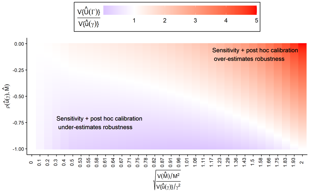
Figure 2: Visualization. This figure visualizes (38) and shows when sensitivity analyses with post hoc calibration over-/under-estimate robustness to unmeasured confounding

Figure 2 helps build further intuition for when standard approaches over-/under-estimate robustness to unmeasured confounding. In the red area in the top-right of Figure 2, standard approaches over-estimate robustness to unmeasured confounding, and confidence intervals for the upper bound on the ATE will be anti-conservative. In the blue area in the bottom-left, standard approaches under-estimate robustness to unmeasured confounding, and confidence intervals for the upper bound on the ATE will be conservative. Along the white diagonal the approaches yield the same conclusions. This plot does not characterize the whole space because it is red for $>2$ on the x-axis and $>0$ on the y-axis (i.e., for most of the space, standard approaches over-estimate robustness to unmeasured confounding). Interpreting both the plot and (39), standard approaches can over-/under-estimate robustness to unmeasured confounding in the following ways:

• Standard methods under-estimate robustness to unmeasured confounding, i.e., $\mathbb{V}\{\widehat{\mathcal{U}}(\Gamma)\}<\mathbb{V}\{\widehat{u}(\gamma)\}$, when

  1. $\widehat{u}(\gamma)$ and $\widehat{M}$ have similar standardized accuracy and are highly negatively correlated, or

  2. $\widehat{u}(\gamma)$ and $\widehat{M}$ are negatively correlated while $\widehat{u}(\gamma)$ has higher standardized accuracy than $\widehat{M}$.

• Standard methods over-estimate robustness to unmeasured confounding, i.e., $\mathbb{V}\{\widehat{\mathcal{U}}(\Gamma)\}>\mathbb{V}\{\widehat{u}(\gamma)\}$, when

  1. $\widehat{u}(\gamma)$ and $\widehat{M}$ are positively correlated, or

  2. The standardized accuracy of $\widehat{u}(\gamma)$ is less than half the standardized accuracy of $\widehat{M}$.

This analysis gives basic intuition for when standard methods might over- or under-estimate robustness to unmeasured confounding by not appropriately accounting for uncertainty in estimates of measured confounding. In the next section, we illustrate these points further and demonstrate the methods for estimation and inference developed in this section with several data analyses. Indeed, we observe that results can be more, or less, robust to unmeasured confounding when accounting for uncertainty in estimating measured confounding.

6 Illustrative Data Analyses

In this section, we illustrate our methods with three data analyses. We revisit two well-studied datasets, which examine the effect of exposure to violence on attitudes towards peace in Darfur and the effect of mothers’ smoking on infant birth weight. We analyze the Darfur and smoking data using the maximum LOO effect differences model and also analyze the Darfur data with the maximum LOO odds ratio model.

6.1 Datasets

6.1.1 Peace attitudes in Darfur

The first dataset contains information about the attitudes towards peace of Darfurian villagers exposed to violence. In 2003 and 2004, the Darfurian government led a series of violent attacks against civilians, killing an estimated two hundred thousand people. Due to the quasi-randomness of the attacks, with this dataset one can attempt to answer the question of whether being directly injured or maimed in such attacks made people more or less likely to accept peace (Hazlett, 2020). We use an example version of this dataset, which is publicly available in the sensemakr package (Cinelli et al., 2020).

The data contains information on 1,276 Darfurian villagers. The treatment is a binary variable indicating whether the individual was physically injured during an attack, and the outcome is an index (continuous from 0 to 1) measuring pro-peace attitudes (with higher being more pro-peace). The covariates include the original village of the respondent (we grouped every village with under 10 respondents into “Other”), gender, age (in years), whether they were a herder or a farmer, whether they voted in an earlier election before the conflict, and the size of their household.

6.1.2 Smoking and birth weight

The second dataset contains information about infant birth weights and mothers’ health in Pennsylvania between 1989 and 1991 (Almond et al., 2005; Cattaneo, 2010). This data has been used to estimate the causal effect of mothers’ smoking on infant birth weight. We used a publicly available dataset consisting of 5,000 randomly subsampled observations from the original dataset (available at https://github.com/mdcattaneo/replication-C_2010_JOE).

The treatment variables takes six values corresponding to ranges of cigarettes smoked daily ($\{0,1-5,6-10,11-15,16-20,>20\}$), but we dichotomize it into whether the mother smoked or not. The outcome variable is the birth weight of the infant in grams. There are a wealth of other covariates, including the race and age of the mother and father, the education level each attained, the mother’s marital status and foreign born status, the county of birth, and indicators for trimester of first prenatal care visit and mother’s alcohol use.

6.2 Methods

We analyzed both datasets assuming the maximum leave-one-out effect differences model (calibrated sensitivity model 1), and also analyzed the Darfur dataset assuming the maximum leave-one-out odds ratio model (calibrated sensitivity model 2).

In the effect differences model, we constructed estimators for the bounds on the ATE according to Definition 1. We constructed estimators for the adjusted mean difference with different covariate subsets using the npcausal package in R (Kennedy, 2023a; R Core Team, 2021). We used 5 splits and estimated the propensity score and outcome regression functions with the SuperLearner, stacking the sample average and a random forest from the ranger package with default tuning parameters (van der Laan et al., 2007; Wright and Ziegler, 2017). We constructed 95% pointwise confidence bands for the upper bound on the ATE with $\Gamma\in\{0.5,1,\dots,5\}$ according to (27), and a 95% pointwise confidence band on the lower bound by an analogous construction (subtracting measured confounding).

In the odds ratio model, we constructed estimators for the bounds on the ATE according to Definitions 2 and 3, with $\exp(\Gamma)\in\{1.25,1.5,1.75,2\}$. We estimated the best projection of measured confounding using a logistic regression with no interactions (see Definition 2). We also assumed that the observed maxima and minima in the covariate data were the true bounds of the covariate support, which allowed us to extend Theorem 2 to a known and bounded support — in this case, we estimated measured confounding with the largest absolute coefficient multiplied by the relevant covariate range. We then estimated the upper bound on the ATE using the algorithm in Yadlowsky et al. (2022), with sieve estimators for the nuisance functions. We constructed 95% confidence bands for the upper and lower bounds using a Wald-type confidence interval, but estimated the variance with the nonparametric bootstrap, with $100$ resampling iterations of size $1000$.

In all three analyses, we also conducted a standard sensitivity analysis and post hoc calibration step, where we standardized the sensitivity parameter by measured confounding.

6.3 Results

6.3.1 Maximum LOO effect differences model

We report the results from the maximum LOO effect differences model first. Two key point estimates in our results are the ATE estimate with all covariates and the estimated maximum LOO measured confounding. Table 2 shows these results for each analysis.

With the Darfur data, we estimated a positive and significant ATE of 0.06 which, interpreted causally, says that exposure to violence increased people’s preference of peace by 0.06 on average (0.06 is a unit-less value — the outcome is an index continuous on $[0,1]$). Moreover, we estimated that the respondent’s original village was the most impactful confounder, and that the absolute change in the adjusted mean difference without it included as a covariate was 0.01. Meanwhile, with the smoking data, we estimated a negative and significant ATE of -272g, which, interpreted causally, says that a mother’s smoking will lower their child’s birth weight by 272g, on average. In addition, we estimated that education of the parents was the most impactful confounder, and that the absolute change in the adjusted mean difference without it included as a covariate was 47g. There is a large degree of uncertainty in the estimate of the impact of education — the lower bound of its 95% confidence interval is zero.

	Violence and peace in Darfur	Smoking and birth weight
ATE estimate and 95% CI	$0.06$, $[0.02,0.10]$	$-272$g, $[-360\text{g},-184\text{g}]$
Variable corresponding to maximum confounding; Estimate and 95% CI	Village $0.01$, $[0.002,0.02]$	Education $47$g, $[0\text{g},118\text{g}]$

Table 2: Average Treatment Effect and maximum measured confounding. For each dataset (columns), this table shows (first row) the ATE estimate and 95% CI and (second row) the variable corresponding to the largest change in the adjusted mean difference when removed, the size of the change, and a 95% CI.

Figure 3 shows the causal effect estimates and 95% confidence bands — Figure 3(a) is for the Darfur data while Figure 3(b) is for the smoking data. The x-axis is the level of the sensitivity parameter, $\Gamma$, in the calibrated sensitivity model, and the sensitivity parameter standardized by estimated measured confounding, $\gamma/\widehat{M}$, in the sensitivity model. The y-axis is at the level of the causal effect. The horizontal black dashed lines are the ATE estimates (also in Table 2), and the horizontal black dotted lines are at zero. The purple lines are the estimates of the upper and lower bounds on the ATE. By the invariance property discussed in Proposition 2 in Section 4, the point estimates for these bounds are the same in the calibrated sensitivity model and sensitivity model. However, the confidence intervals for the bounds differ. The confidence intervals for the calibrated sensitivity model are in red, while the confidence intervals for the sensitivity model are in blue.

The calibrated sensitivity results in Figure 3(a) can be interpreted in the following way. The estimated bounds on the ATE do not intersect zero for unmeasured confounding less than five times measured confounding, and the confidence interval for the ATE intersects zero when $\Gamma\approx 2$, so the statistical significance of the estimated effect would only be nullified for unmeasured confounding twice as big as measured confounding. In this case, the measured confounding is the maximum change in the adjusted mean difference from leaving out one covariate. The most impactful observed confounder was the respondent’s home village, and it changed the adjusted mean difference by 0.01. The results in Figure 3(b) can be interpreted similarly.

While both the traditional and calibrated sensitivity analyses suggest that each effect is somewhat robust to confounding, they suggest it to differing degrees. Indeed, these results illustrate how not accounting for uncertainty in estimating measured confounding can lead to over- or under-estimating robustness to unmeasured confounding. In Figure 3(a), the calibrated sensitivity model confidence intervals always contain the sensitivity model confidence intervals. Therefore, the standard analysis over-estimates robustness to unmeasured confounding. Similar trends arise in Figure 3(b). However, for $\Gamma<2$, the calibrated CI is tighter on the upper bound, and thus could lead to concluding the effect estimate is more robust to unmeasured confounding, at least for $\Gamma<2$.

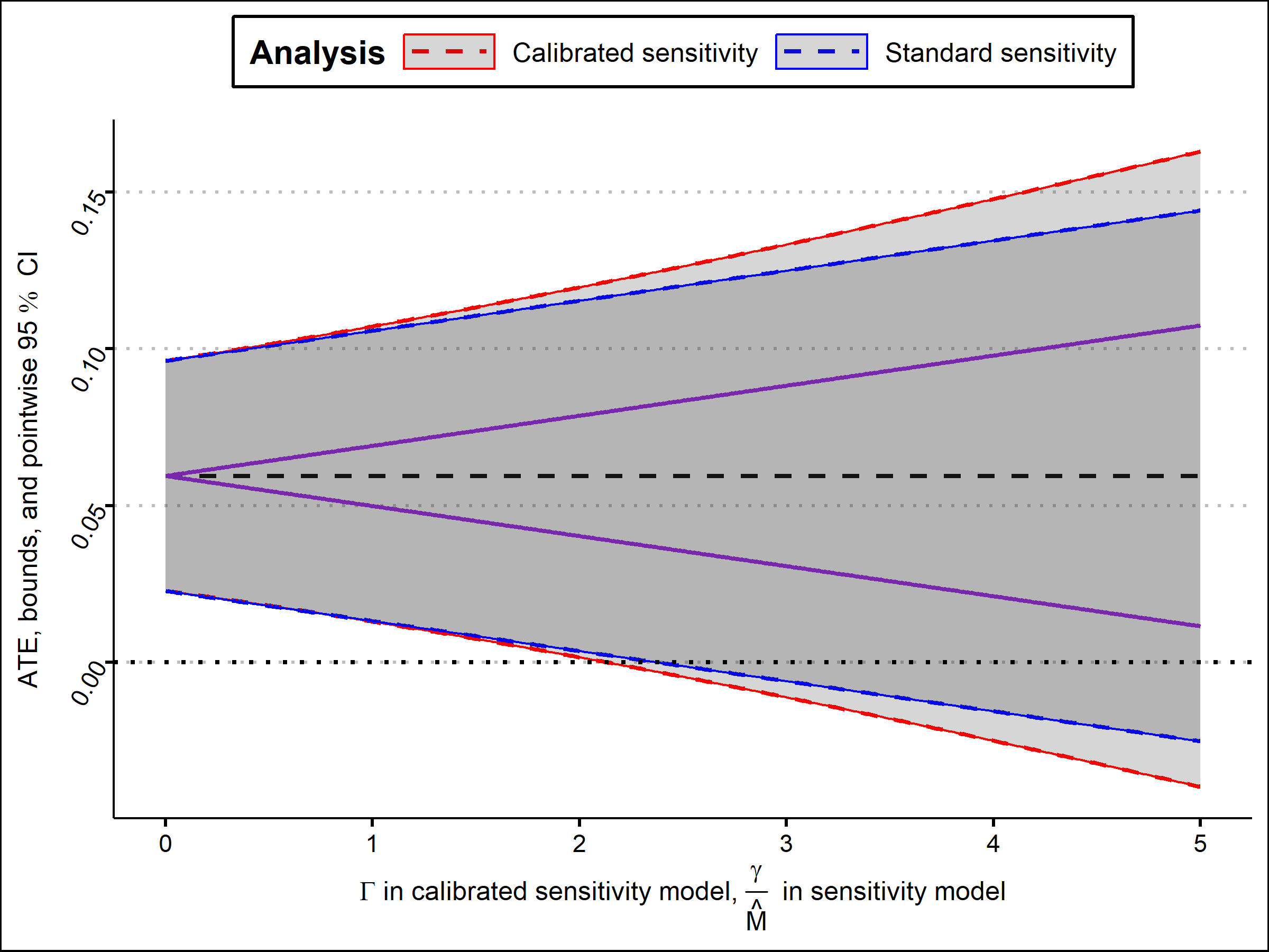
(a) The effect of exposure to violence on preference for peace in Darfur.

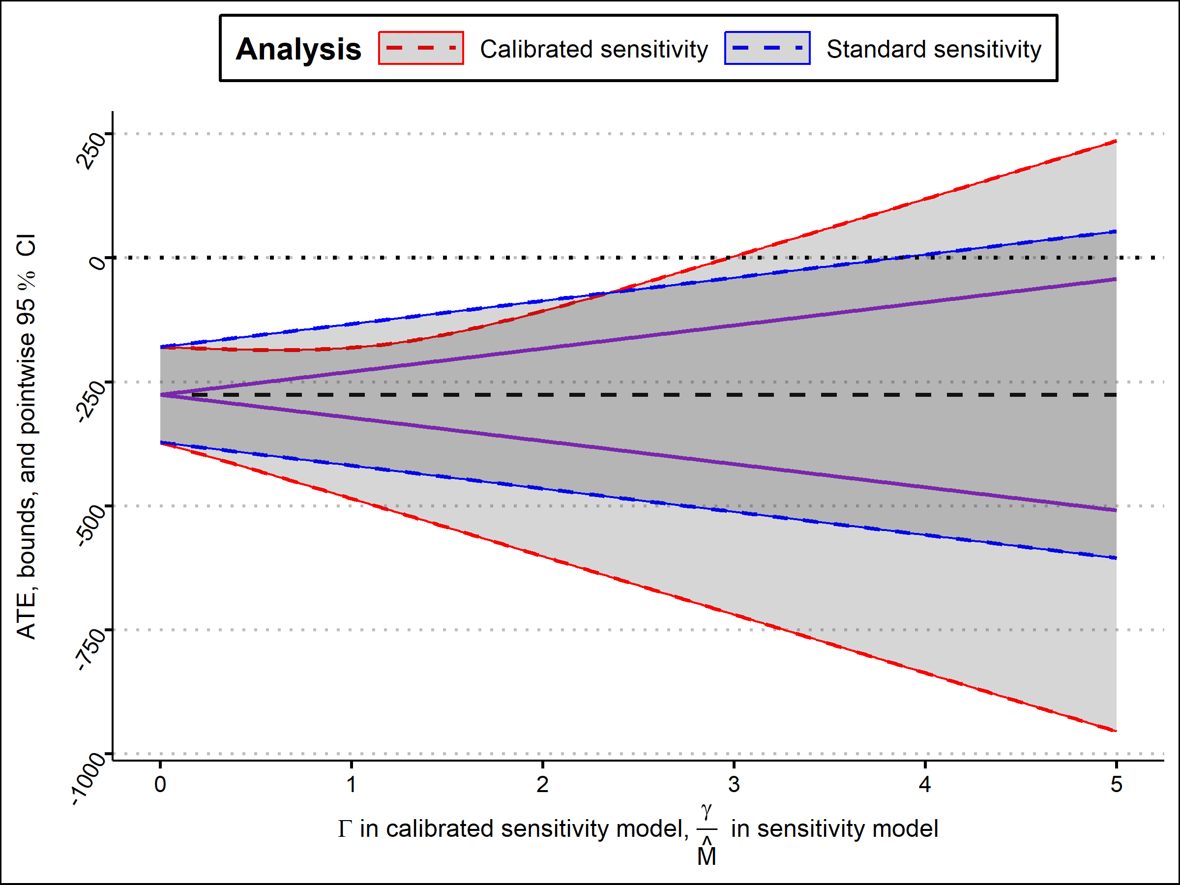
(b) The effect of mothers’ smoking on infant birth weight.

Figure 3: Average Treatment Effect and pointwise 95% confidence interval. These figures show the ATE estimate and 95% confidence intervals (y-axis) at different levels of unmeasured confounding (x-axis).

6.4 Maximum LOO odds ratio model

This section reports the results from the maximum LOO odds ratio model and the Darfur data. The relationship between the calibrated sensitivity results and standard sensitivity results are similar to before, in the sense that incorporating uncertainty due to estimating measured confounding demonstrates that the causal effect estimate is less robust unmeasured confounding. However, with both the traditional and calibrated sensitivity models, the odds ratio model suggests the estimates are far less robust to unmeasured confounding than the effect differences model did.

The ATE estimate and confidence interval are the same, still roughly 0.6 and $[0.02,0.1]$ (see Table 2), and the maximum LOO confounder is still village. However, neither method, sensitivity or calibrated sensitivity, suggests the results are robust to unmeasured confounding. First, without standardizing by measured confounding, the confidence interval in the standard sensitivity model intersects the x-axis for $\gamma\approx 0.11$ (multiplying the point where the blue lines in Figure 4 intersect the x-axis by the estimate for measured confounding $\widehat{M}$). On the exponential scale, which this model is usually expressed in, that corresponds to a sensitivity parameter of roughly $1.12$. Arguably, this indicates much less robustness to unmeasured confounding than was observed in the the effect differences analysis. The lack of robustness to unmeasured confounding may be an artifact of the estimation process — for computational simplicity, we manually constructed sieve estimators for the nuisance functions $\nu_{a}^{\pm}$ and $\theta_{a}^{\pm}$ using a linear model with no interactions. This may be a poor approximation of the true functions, and more careful estimation here could lead to different results.

When maximum LOO confounding is incorporated, the results become even less robust to unmeasured confounding, because the maximum LOO confounding is high and has high variance. The maximum estimated confounding is $3.34$, with a huge confidence interval of $[0,20]$ (this is a Wald-type confidence interval truncated below at $0$ where the variance was calculated across $100$ bootstrap resamples). As a result, the calibrated confidence intervals intersect the x-axis for $\Gamma\approx 0.025$, suggesting unmeasured confounding which is only a small multiple of measured confounding would be enough to overturn the conclusions of the study.

The estimated measured confounding may be high because the best projection estimator is a poor approximation of the true propensity score. The high variance across bootstrap resamples reinforces this and suggests this estimator is unstable. More generally, understanding why these results indicate such different conclusions from the effect differences analysis is a topic of future work.

Variable corresponding to maximum confounding	Estimate and 95% confidence interval for measured confounding
Village	$3.34$,     $[0,20]$

Table 3: Measured confounding. The variable corresponding to the largest change in the log odds ratio of the propensity score when removed, the size of the change, and a 95% CI from bootstrap resampling.

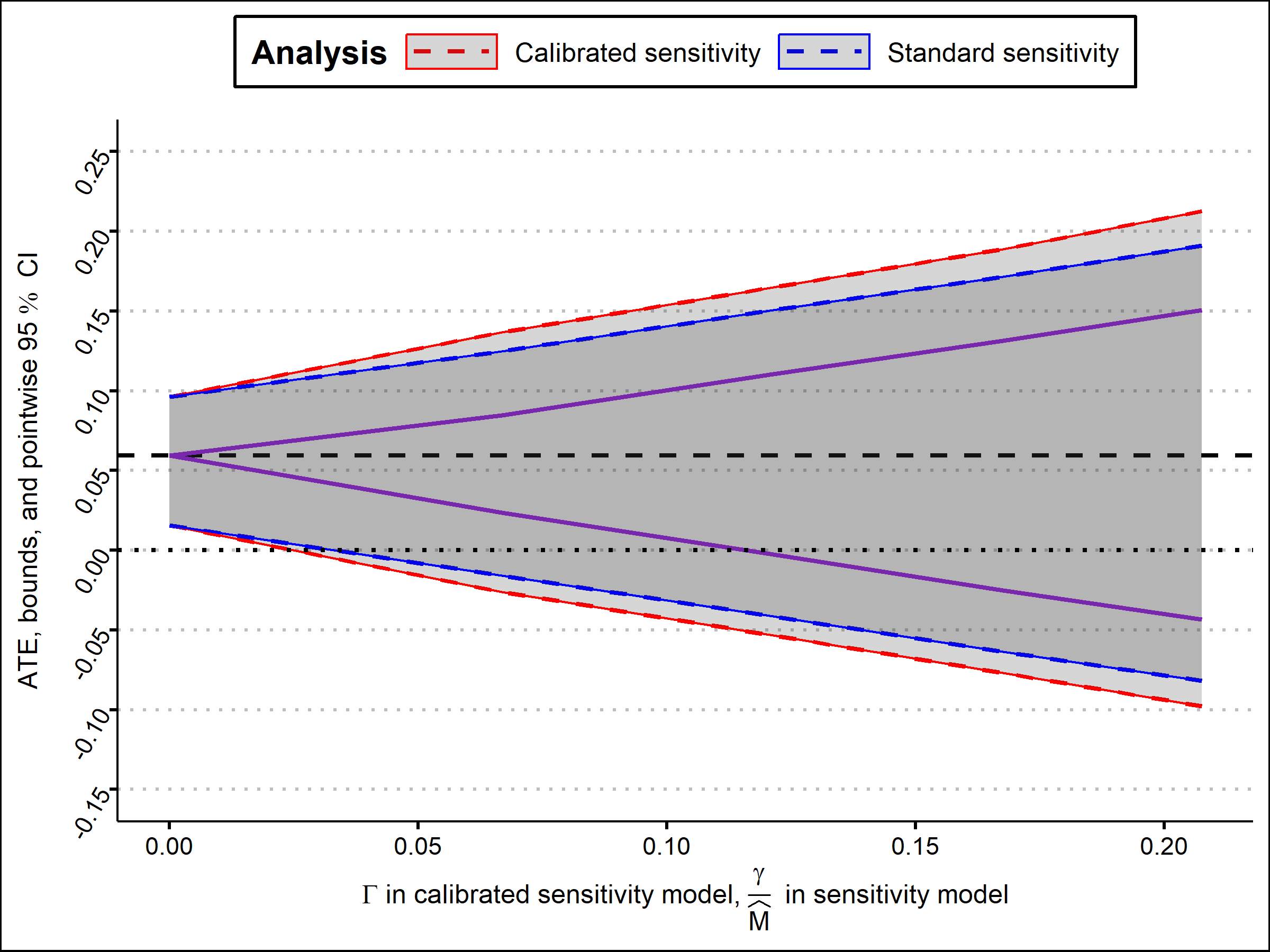
Figure 4: Average Treatment Effect and pointwise 95% confidence interval. The ATE estimate and 95% confidence intervals (y-axis) at different levels of unmeasured confounding (x-axis).

7 Discussion

In this paper, we introduced calibrated sensitivity models to estimate nonparametric bounds on causal effects while allowing for unmeasured confounding. Calibrated sensitivity models bound the error due to unmeasured confounding by a multiple of measured confounding. We demonstrated that calibrated sensitivity analyses have several advantages over traditional sensitivity analyses and post hoc calibration analyses, including (1) the calibrated sensitivity parameter has an intuitive unit-less definition as the ratio of unmeasured over measured confounding, unlike standard sensitivity parameters; (2) uncertainty in the estimate for measured confounding can be incorporated correctly, which prior methods failed to do; and (3) new quantifications of unmeasured confounding, which may have advantages over standard methods (e.g., more flexible, simpler), can be bounded in an intuitive manner. Moreover, we also noted that the choice of measured confounding, which is often unjustified in standard post hoc calibration, might be better justified in practice with calibrated sensitivity models, because the metric for measured confounding is an assumption within the calibrated sensitivity model itself, rather than a choice that’s made after the sensitivity analysis is conducted.

We provided intuition for calibrated sensitivity models through several examples, using different quantifications of unmeasured confounding and showing how to justify different quantifications of measured confounding. Then, we identified bounds on the average treatment effect and derived methods for estimation and inference for those bounds which account for uncertainty in estimated measured confounding. We established when the estimators are $\sqrt{n}$-consistent and asymptotically normal under doubly robust style conditions on their nuisance function estimators. Finally, we conducted data analyses to illustrate these methods, examining the effect of exposure to violence on attitudes towards peace in Darfur and the effect of mothers’ smoking on infant birth weight. By correctly incorporating uncertainty due to estimating measured confounding, we observe that causal effect can less robust or more robust to unmeasured confounding that would have been shown with standard approaches.

There are several limitations to this approach. First, from a wider causal perspective, this method still requires an untestable assumption about unmeasured confounding (relating it to measured confounding). Other approaches, such as instrumental variables or regression discontinuity designs, may be better for particular applications. Second, from a statistical perspective, calibrated sensitivity analyses require an accurate estimator for both measured confounding and the resulting bounds on the effect, whereas an un-calibrated sensitivity model only requires an accurate estimator for the bounds on the effect. Nonetheless, the advantages of calibrated sensitivity analyses over standard methods may outweigh these disadvantages, particularly because both disadvantages also apply to standard post hoc calibration analyses.

There are several natural directions for future work. First, other model choices are possible within the partial identification framework we considered. Therefore, an interesting avenue for future work is establishing further theoretical and inferential results for other partial identification calibrated sensitivity models. Second, a natural extension of this work would be to examine one-number summaries of effect sensitivity in further detail, such as the minimum value of the sensitivity parameter that would reverse the conclusions of the analysis. Finally, two promising avenues include developing calibrated sensitivity models that point identify causal effects, and extending these methods to conduct calibrated sensitivity analyses for violations of other assumptions, such as covariate shift (Rothenhäusler and Bühlmann, 2023).

References

Appendix

This appendix is split into four sections:

1. provides results for Section 4, Proposition 1 and Lemma 2.

2. provides the relevant efficient influence functions for estimating measured confounding and the bounds, deriving new efficient influence functions for the outcome model.

3. provides results for Section 5; in particular, for the convergence results in Theorems 1-3.

4. provides a technical result for estimating the maximum of a finite number of functionals, which is used in the proofs in Appendix C.

Appendix A Results in Section 4

Proposition 1

Proof:

The proof follows for the effect differences model directly from the definition of the model, while for the odds ratio model it follows by Yadlowsky et al. [2022] Lemma 2.1.

For the outcome model,

$$\mathbb{E}(Y^{1}-Y^{0}) =\mathbb{E}\left\{\mathbb{E}(Y^{1}-Y^{0}\mid X)\right\}$$

$$=\mathbb{E}\left\{\mathbb{E}(Y^{1}-Y^{0}\mid A=1,X)\pi_{1}(X)+\mathbb{E}(Y^{1}-Y^{0}\mid A=0,X)\pi_{0}(X)\right\}$$

$$=\mathbb{E}\{\mathbb{E}(Y^{1}\mid A=1,X)-\mathbb{E}(Y^{0}\mid A=0,X)\}$$

$$\hskip 14.45377pt-\mathbb{E}\left\{\mathbb{E}(Y^{1}\mid A=1,X)\pi_{0}(X)+\mathbb{E}(Y^{0}\mid A=1,X)\pi_{1}(X)\right\}$$

$$\hskip 14.45377pt+\mathbb{E}\left\{\mathbb{E}(Y^{1}\mid A=0,X)\pi_{0}(X)+\mathbb{E}(Y^{0}\mid A=0,X)\pi_{1}(X)\right\}$$

$$=\psi+\sum_{a\in\{0,1\}}(2a-1)\mathbb{E}\left[\left\{\mathbb{E}(Y^{a}\mid A=1-a,X)-\mu_{a}(X)\right\}\pi_{1-a}(X)\right].$$

Therefore, by Hölder’s inequality,

$$\left|\psi^{\ast}-\psi^{[d]}\right|\leq\sum_{a\in\{0,1\}}\Big{\lVert}\mathbb{E}(Y^{a}\mid A=1-a,X)-\mu_{a}(X)\Big{\rVert}_{p}\Big{\lVert}\pi_{1-a}(X)\Big{\rVert}_{r}$$

where $r=1$ if $p=\infty$ and $r=\frac{p}{p-1}$ otherwise. Under calibrated sensitivity model 3, the result follows by setting $p=r=2$ and imposing the model. $\square$

Proposition 2

Proof:

The calibrated sensitivity model imposes the bound $U\leq\Gamma M$. Because $\Gamma\in\mathbb{R}^{+}$ and $0<M<\infty$ by assumption, $\Gamma M\in\mathbb{R}^{+}$. Therefore, this model implies an upper bound on the causal effect of interest: $u(\Gamma M)$ (substitute $\gamma^{\prime}=\Gamma M$ and use the assumption/construction of the sensitivity model). Because $u(\cdot)$ is a deterministic function, it maps the same inputs to the same outputs, and the result follows. $\square$

A.1 Differentiability with the odds ratio model

Here, we provide the details on the derivatives considered implicitly in Lemma 1. For analyzing the odds ratio model, we require several mild continuity and boundedness assumptions. For this purpose, we define one more nuisance function and a loss function:

$$\omega_{\theta}(Y;t) :=\big{(}Y-\theta\big{)}\mathbbold{1}\big{(}Y>\theta\big{)}+t\big{(}Y-\theta\big{)}\mathbbold{1}\big{(}Y<\theta\big{)}\text{ and }$$ (40)

$$\ell_{t}(\theta,y) :=\frac{1}{2}\Big{[}\big{\{}(y-\theta)\mathbbold{1}(y>\theta)\big{\}}^{2}+t\big{\{}(y-\theta)\mathbbold{1}(y<\theta)\}^{2}\Big{]}.$$ (41)

Next, we give the continuity and boundedness conditions required (see Lemmas 2.2 and 2.3 and Assumption A.1 in Yadlowsky et al. [2022]).

Assumption 7.

Smooth and bounded data generating process:

1. $f(x)$, the covariate density, $\pi_{1}(x)$, and $\theta_{1}^{-}(x;t)$ (defined in (19)) are continuous in $x$,

2. For $a\in\{0,1\}$, $p(y\mid A=a,x)$, the conditional density of $Y$ given $A=a$ and $X=x$ is continuous in $y$ and $x$, upper bounded, and has bounded support,

3. $Y$ is bounded,

4. $\theta_{a}^{\pm}(x;t)$ is bounded for bounded $t$ and is absolutely integrable in $x$, and

5. $(r,x)\mapsto\mathbb{E}\left\{\ell_{\exp(\Gamma M)}\big{(}r,Y\big{)}\mid A=a,x\right\}$ is continuous in $r$ and $x$ and
   $\mathbb{E}\left(\ell_{\exp(\Gamma M)}\Big{[}\theta_{a}^{\pm}\{X;\exp(\Gamma M)\},Y\Big{]}\mid A=1,x\right)<\infty$.

This assumption imposes mild continuity and boundedness conditions. Condition 1, the continuity of $p(y\mid A=a,x)$, the boundedness of $Y$, and the absolute integrability of $\theta_{a}^{\pm}$ are beyond what is assumed in Yadlowsky et al. [2022]. Condition 2 is contained in Assumption A.1 of that paper, while the first half of condition 4 is in Lemma 2.2 and condition 5 is in Lemma 2.3. With this assumption in hand, we can now state and prove the following result — Lemma 2 — which implies Lemma 1.

Lemma 2.

(Differentiable bounds in the odds ratio model) Under the setup of Lemma 1,

$$\frac{\partial}{\partial M}\mathcal{L}(\Gamma) =-\Gamma\exp(\Gamma M)\mathbb{E}\left\{\frac{\pi_{0}(X)f_{1}(X;\theta_{1}^{-})}{\nu_{1}^{-}(X)}\right\}-\Gamma\mathbb{E}\left\{\pi_{1}(X)\frac{\widetilde{f}_{0}(X;\theta_{0}^{+})}{\nu_{0}^{+}(X)}\right\}\text{ and }$$ (42)

$$\frac{\partial}{\partial M}\mathcal{U}(\Gamma) =\Gamma\mathbb{E}\left\{\pi_{0}(X)\frac{\widetilde{f}_{1}(X;\theta_{1}^{+})}{\nu_{1}^{+}(X)}\right\}+\Gamma\exp(\Gamma M)\mathbb{E}\left\{\pi_{1}(X)\frac{f_{0}(X;\theta_{0}^{-})}{\nu_{0}^{-}(X)}\right\},$$ (43)

where $X\equiv X$; $\theta_{a}^{\pm}\equiv\theta_{a}^{\pm}\{X;\exp(\Gamma M)\}$; $\theta_{a}^{\pm}$ and $M$ are defined in (19) and (20), respectively; and

$$f_{a}(x;\theta) =\mathbb{E}\left\{\left(\theta-Y\right)\mathbbold{1}\left(\theta>Y\right)\mid A=a,X=x\right\},$$ (44)

$$\widetilde{f}_{a}(x;\theta) =\mathbb{E}\big{\{}(Y-\theta)\mathbbold{1}(Y>\theta)\mid A=a,X=x\big{\}},$$ (45)

$$\nu_{a}^{-}(x)\equiv\nu_{a}^{-}\{x;\theta,t=\exp(\Gamma M)\} =\mathbb{P}(Y\geq\theta\mid A=a,X=x)+t\mathbb{P}(Y<\theta\mid A=a,X=x)\text{, and}$$ (46)

$$\nu_{a}^{+}(x)\equiv\nu_{a}^{+}\{x;\theta,t=\exp(\Gamma M)\} =\mathbb{P}(Y>\theta\mid A=a,X=x)+\frac{1}{t}\mathbb{P}(Y<\theta\mid A=a,X=x).$$ (47)

Moreover, the derivative of the upper bound is positive and bounded while the the derivative of the lower bounds is negative and bounded.

Proof:

The derivatives for the upper and lower bounds on $\mathbb{E}(Y^{1})$ follow from this proof and the four lemmas afterward. The other derivatives for the upper and lower bounds on $\mathbb{E}(Y^{0})$ follow the same argument, but replacing $A=1$ by $A=0$. Note that, by assumption $0<\exp(\Gamma M)<\infty$. Hence, Lemmas 3, 4, 5, and 6 apply, and the result then follows by the chain rule, Assumption 2 and the dominated convergence theorem (to bring the derivative inside the expectation), and canceling terms. The boundedness of the derivative follows because $\widetilde{f}_{a},f_{a},\nu_{a}^{\pm}$ are all bounded and $M$ and $\Gamma$ are non-zero and bounded by assumption. The sign follows because $f_{a},\widetilde{f}_{a},\nu_{a}^{\pm}>0$. $\square$

Lemma 3.

Under the setup of Lemma 2, for $t^{\prime}>0$,

$$\frac{\partial}{\partial t}\theta_{1}^{-}(X;t)\Big{|}_{t=t^{\prime}}=-\frac{f_{1}(X;\theta_{1}^{-})^{2}}{g_{1}\big{(}X;\theta_{1}^{-}\big{)}},$$ (48)

where $X\equiv X$, $\theta_{1}^{-}:=\theta_{1}^{-}(X;t^{\prime})$ on the right-hand side, $f_{a}(x;\theta)$ is defined in (44), and

$$g_{a}(x;\theta)=f_{a}(x;\theta)\mathbb{P}\left(Y>\theta\mid A=a,X=x\right)+\widetilde{f}_{a}(x;\theta)\mathbb{P}\left(Y<\theta\mid A=a,X=x\right),$$ (49)

where $\widetilde{f}$ is defined in (45).

Proof:

We establish the result using the inverse function theorem, where we express $t$ as a function of $\theta$.

Under Assumption 7, Lemma 2.3 from Yadlowsky et al. [2022] applies, such that $\theta_{1}^{-}(X;t)$ is the unique minimizer (up to measure-zero sets) of $\mathbb{E}\{\ell_{t}(\theta,Y)\mid A=1,X\}$ and solves

$$\mathbb{E}\{\omega_{\theta_{1}^{-}(X;t)}(Y;t)\mid A=1,X\}=0$$ (50)

In what follows let $\theta\equiv\theta_{1}^{-}(X;t)$ to further simplify notation. The moment condition implies

$$t(\theta)=\frac{\mathbb{E}\big{\{}(Y-\theta)\mathbbold{1}(Y>\theta)\mid A=1,X=x\big{\}}}{\mathbb{E}\big{\{}(\theta-Y)\mathbbold{1}(\theta>Y)\mid A=1,X=x\big{\}}}.$$ (51)

It is possible to divide by $\mathbb{E}\big{\{}(\theta-Y)\mathbbold{1}(\theta>Y)\mid A=1,X=x\big{\}}$ when $t>0$ because

1. $\mathbb{E}\big{\{}(Y-\theta)\mathbbold{1}(Y>\theta)\mid A=1,X=x\big{\}}$ and $\mathbb{E}\big{\{}(\theta-Y)\mathbbold{1}(\theta>Y)\mid A=1,X=x\big{\}}$ are both non-negative by definition, and

2. $\mathbb{E}\big{\{}(Y-\theta)\mathbbold{1}(Y>\theta)\mid A=1,X=x\big{\}}$ and $\mathbb{E}\big{\{}(\theta-Y)\mathbbold{1}(\theta>Y)\mid A=1,X=x\big{\}}$ cannot each be zero simultaneously because $p(y\mid A=1,x)$ is continuous and upper bounded, which implies $Y\mid A=1,X=x$ is not a point mass.

From 1. and 2., we conclude both $\mathbb{E}\big{\{}(Y-\theta)\mathbbold{1}(Y>\theta)\mid A=1,X=x\big{\}}$ and $\mathbb{E}\big{\{}(\theta-Y)\mathbbold{1}(\theta>Y)\mid A=1,X=x\big{\}}$ must be positive.

By the continuity assumption on $p(y\mid A=1,x)$ and the quotient rule and Leibniz’ integral rule (see Lemma 5 for specific steps), we can take the derivative of $t(\theta)$ wrt $\theta$, and find

$$\frac{\partial}{\partial\theta}t(\theta):=-\Bigg{(} \frac{\mathbb{E}\big{\{}(\theta-Y)\mathbbold{1}(\theta>Y)\mid A=1,X=x\big{\}}\mathbb{E}(Y\geq\theta\mid A=1,X=x)}{\Big{[}\mathbb{E}\big{\{}(\theta-Y)\mathbbold{1}(\theta>Y)\mid A=1,X=x\big{\}}\Big{]}^{2}}$$

$$+\frac{\mathbb{E}\big{\{}(Y-\theta)\mathbbold{1}(Y>\theta)\mid A=1,X=x\big{\}}\mathbb{E}(Y\leq\theta\mid A=1,X=x)}{\Big{[}\mathbb{E}\big{\{}(\theta-Y)\mathbbold{1}(\theta>Y)\mid A=1,X=x\big{\}}\Big{]}^{2}}\Bigg{)}$$ (52)

Notice that the denominator is positive by the prior argument, while the numerator is also positive by the prior argument and because $\mathbb{E}(Y\geq\theta\mid A=1,X=x)\wedge\mathbb{E}(Y\leq\theta\mid A=1,X=x)>0$ by the same argument regarding the continuity of $p(y\mid A=1,x)$. Moreover, both the numerator and denominator are bounded by Assumption 7.

Hence, $\frac{\partial}{\partial\theta}t(\theta)$ exists and is always negative and bounded. Therefore, the result follows by the inverse function theorem for the reciprocal of (52). Moreover, $\frac{\partial}{\partial t}\theta(t)$ is continuous because $p(y\mid A=1,x)$ is continuous and $\frac{\partial}{\partial\theta}t(\theta)$ is a composition of integrals of $p(y\mid A=1,x)$. $\square$

Lemma 4.

Under the setup of Lemma 2, then

$$\nu_{1}^{-}\big{(}X;\theta_{1}^{-},t\big{)}f_{1}(X;\theta_{1}^{-})=g_{1}\big{(}X;\theta_{1}^{-},t\big{)}$$ (53)

where $X\equiv X$, $\theta_{1}^{-}:=\theta_{1}^{-}(X;t)$, and $\nu_{1}^{-}(X,\theta,t)$, $f_{a}(x;\theta)$, and $g_{a}(X;\theta,t)$ are defined in (46), (44), and (49), respectively.

Proof:

Omitting arguments, on the left-hand side of (53) we have

$$\nu f_{1}=f_{1}\mathbb{P}(Y\geq\theta\mid A=1,X=x)+tf_{1}\mathbb{P}(Y\leq\theta\mid A=1,X=x).$$ (54)

For the second summand on the right-hand side of (54),

$$tf_{1}\mathbb{P}(Y\leq\theta\mid A=1,X=x) =t\mathbb{E}\left\{\left(\theta-Y\right)\mathbbold{1}\left(\theta>Y\right)\mid A=a,X=x\right\}\mathbb{P}(Y\leq\theta\mid A=1,X=x)$$

$$=-t\mathbb{E}\left\{\left(Y-\theta\right)\mathbbold{1}\left(\theta>Y\right)\mid A=a,X=x\right\}\mathbb{P}(Y\leq\theta\mid A=1,X=x)$$

$$=\mathbb{E}\left\{\left(Y-\theta\right)\mathbbold{1}\left(Y>\theta\right)\mid A=a,X=x\right\}\mathbb{P}(Y\leq\theta\mid A=1,X=x)$$

where the third equality follows because $\theta$ solves the moment equation $\mathbb{E}(\omega_{\theta}(Y)\mid A=1,X=x)=0$ (see, (50)). Hence,

$$\nu f_{1} =f_{1}\mathbb{P}(Y\geq\theta\mid A=1,X=x)$$

$$+\mathbb{E}\left\{\left(Y-\theta\right)\mathbbold{1}\left(Y>\theta\right)\mid A=a,X=x\right\}\mathbb{P}(Y\leq\theta\mid A=1,X=x)$$

$$=g_{1}(X;\theta).$$

$\square$

Lemma 5.

Under the setup of Lemma 2,

$$\frac{\partial}{\partial\theta}\mathbb{E}\{(Y-\theta)\mathbbold{1}(Y>\theta)\mid A=a,X=x\} =-\mathbb{P}(Y>\theta\mid A=a,X=x)$$ (55)

$$\frac{\partial}{\partial\theta}\mathbb{E}\{(\theta-Y)\mathbbold{1}(\theta\geq Y)\mid A=a,X=x\} =\mathbb{P}(Y\leq\theta\mid A=a,X)$$ (56)

Proof:

By the continuity assumption on $p(y\mid A=a,x)$, the boundedness of $Y$, and Leibniz’ integral rule,

$$\frac{\partial}{\partial\theta}\mathbb{E}\{(Y-\theta)\mathbbold{1}(Y>\theta)\mid A=a,X=x\} \equiv\frac{\partial}{\partial\theta}\int_{\theta}^{\overline{B}}(Y-\theta)p(y\mid A=a,x)dy$$

$$=0+\int_{\theta}^{\overline{B}}\frac{\partial}{\partial\theta}(Y-\theta)p(y\mid A=a,x)dy$$

$$=-\int_{\theta}^{\overline{B}}p(y\mid A=a,x)dy$$

$$=-\mathbb{P}(Y>\theta\mid A=a,X=x),$$

where $\overline{B}$ is the upper bound on $Y$, and

$$\frac{\partial}{\partial\theta}\mathbb{E}\{(\theta-Y)\mathbbold{1}(\theta\geq Y)\mid A=a,X=x\} =\int_{\underline{B}}^{\theta}\frac{\partial}{\partial\theta}(\theta-Y)p(y\mid A=a,x)dy$$

$$=\mathbb{P}(Y\leq\theta\mid A=a,X=x),$$

where $\underline{B}$ is the lower bound on $Y$. $\square$

Lemma 6.

Under the setup of Lemma 2, for $t^{\prime}>0$,

$$\frac{\partial}{\partial t}\theta_{1}^{+}(X;t)\Big{|}_{t=t^{\prime}}=\frac{\widetilde{f}_{1}(X;\theta_{1}^{+})^{2}}{g_{1}(X;\theta_{1}^{+})}=\frac{\widetilde{f}_{1}(X;\theta_{1}^{+})}{t^{\prime}\nu_{1}^{+}\big{(}X;\theta_{1}^{+},t^{\prime}\big{)}},$$ (57)

where $X\equiv X$, $\theta_{1}^{+}:=\theta_{1}^{+}(X;t^{\prime})$ on the right-hand side, and $\widetilde{f}_{a}(x;\theta)$, $g_{a}(x;\theta)$ and $\nu_{a}^{+}$ are defined in (45), (49), and (47), respectively.

Proof:

By the same argument as in Yadlowsky et al. [2022] (see, Section 2.3), $\theta_{1}^{+}(X;t)$ minimizes $\mathbb{E}\{\ell_{1/t}(\theta,Y)\mid A=1,X\}$ and solves the moment condition

$$\mathbb{E}\left\{\left(Y-\theta\right)\mathbbold{1}\left(Y>\theta\right)\mid A=1,X=x\right\}-\frac{1}{t}\mathbb{E}\left\{\left(\theta-Y\right)\mathbbold{1}\left(\theta>Y\right)\mid A=1,X=x\right\}=0.$$

Therefore, the first result follows by the same arguments as in Lemma 3 using the inverse function theorem.

For the second result, omitting $X$ arguments and letting $\theta\equiv\theta_{1}^{+}$,

$$\frac{\widetilde{f}_{1}(\theta;t^{\prime})}{\frac{\partial}{\partial y}\theta_{1}^{+}} =\frac{g_{1}(\theta;t^{\prime})}{\widetilde{f}_{1}(\theta;t^{\prime})}$$

$$=\frac{\mathbb{E}\left\{\left(\theta-Y\right)\mathbbold{1}\left(\theta>Y\right)\mid A=1,X=x\right\}\mathbb{E}\left(Y\geq\theta\mid A=1,X=x\right)}{\mathbb{P}\left\{\left(Y-\theta\right)\mathbbold{1}\left(Y>\theta\right)\mid A=1,X=x\right\}}$$

$$+\frac{\mathbb{E}\left\{\left(Y-\theta\right)\mathbbold{1}\left(Y>\theta\right)\mid A=1,X=x\right\}\mathbb{P}\left(Y\leq\theta\mid A=1,X=x\right)}{\mathbb{E}\left\{\left(Y-\theta\right)\mathbbold{1}\left(Y>\theta\right)\mid A=1,X=x\right\}}$$

$$=\frac{\mathbb{E}\left\{\left(\theta-Y\right)\mathbbold{1}\left(\theta>Y\right)\mid A=1,X=x\right\}}{\mathbb{E}\left\{\left(Y-\theta\right)\mathbbold{1}\left(Y>\theta\right)\mid A=1,X=x\right\}}\mathbb{P}\left(Y\geq\theta\mid A=1,X=x\right)+\mathbb{P}(Y\leq\theta\mid A=1,X=x).$$

Because $\theta_{1}^{+}$ solves the moment equation

$$\mathbb{E}\left\{\left(Y-\theta\right)\mathbbold{1}\left(Y>\theta\right)\mid A=1,X=x\right\}-\frac{1}{t^{\prime}}\mathbb{E}\left\{\left(\theta-Y\right)\mathbbold{1}\left(\theta>Y\right)\mid A=1,X=x\right\}=0$$

we have

$$\frac{\widetilde{f}_{1}(\theta;t^{\prime})}{\frac{\partial}{\partial y}\theta_{1}^{+}}=t^{\prime}\mathbb{P}\left(Y>\theta\mid A=1,X=x\right)+\mathbb{P}\left(Y<\theta\mid A=1,X=x\right)=t^{\prime}\nu_{1}^{+}\{X;\theta_{1}^{+}(X;t^{\prime}),t^{\prime}\}.$$

The result follows by rearranging. $\square$

Lemma 1

Note that Lemma 1 follows from Lemma 2.

Appendix B Efficient Influence Functions

To construct doubly robust-style estimators for the bounds on the ATE we will use, when possible, the efficient influence functions (EIFs) for each part of the bound. The EIF is a concept from semiparametric efficiency theory [Bickel et al., 1993, van der Vaart, 2000, Tsiatis, 2006, van der Vaart, 2002, Van der Laan and Robins, 2003], and can be thought of as the first derivative in a von Mises expansion of an estimand [Mises, 1947]. The crucial benefit of the EIF is that estimators constructed from it are doubly robust, in the sense that they have bias that is a second-order product of errors of the relevant nuisance function estimators, so they can achieve $\sqrt{n}$-efficiency even when the nuisance functions are estimated at slower nonparametric rates [Van der Laan and Robins, 2003, Chernozhukov et al., 2018, Kennedy, 2022].

B.1 Effect differences

For the maximum LOO effects differences model (calibrated sensitivity model 1), we only require the EIF of the adjusted mean difference, provided in (26) in the body of the paper.

B.2 Odds ratio

For the maximum LOO odds ratio model (calibrated sensitivity model 2), we can use the EIF from Yadlowsky et al. [2022] for the bounds (see, e.g., (59) for the EIF of the lower bound on $\mathbb{E}(Y^{1})$). The efficient influence function for the upper bound on the ATE is

$$\varphi_{U}\{Z;\eta(\Gamma M)\} :=AY+(1-A)\theta_{1}^{+}\{X;\exp(\Gamma M)\}+A\frac{\omega_{\theta_{1}^{+}}(Y;\exp(\Gamma M))\pi_{0}(X)}{\nu_{1}^{+}\{X;\theta_{1}^{+},\exp(\Gamma M)\}\pi_{1}(X)}$$

$$-(1-A)Y+A\theta_{0}^{-}\{X;\exp(\Gamma M)\}+(1-A)\frac{\omega_{\theta_{0}^{-}}(Y;\exp(\Gamma M))\pi_{1}(X)}{\nu_{0}^{-}\{X;\theta_{1}^{+},\exp(\Gamma M)\}\pi_{0}(X)}$$ (58)

Meanwhile, the efficient influence function for the lower bound on the ATE is

$$\varphi_{L}\{Z;\eta(\Gamma M)\} :=AY+(1-A)\theta_{1}^{-}\{X;\exp(\Gamma M)\}+A\frac{\omega_{\theta_{1}^{-}}\{Y;\exp(\Gamma M)\}\pi_{0}(X)}{\nu_{1}^{-}\{X;\theta_{1}^{-},\exp(\Gamma M)\}\pi_{1}(X)}$$

$$-(1-A)Y+A\theta_{0}^{+}\{X;\exp(\Gamma M)\}+(1-A)\frac{\omega_{\theta_{0}^{+}}\{Y;\exp(\Gamma M)\}\pi_{1}(X)}{\nu_{0}^{+}\{X;\theta_{1}^{+},\exp(\Gamma M)\}\pi_{0}(X)}$$ (59)

where $\theta^{\pm},\nu^{\pm}$, and $\omega$ are defined in (19), (46), (47), and (40).

Because the measured confounding is a supremum, it is not pathwise differentiable and does not admit an EIF (see, e.g., Hines et al. [2022] for discussion of a lack of pathwise differentiability). Instead, we estimated its projection onto a finite dimensional model, which can be estimated at a $\sqrt{n}$-rate with a plug-in estimator, as in Definition 2.

B.3 Outcome model

The average LSO outcome model (calibrated sensitivity model 3) requires the derivation of two EIFs, for each multiplicand in the bounds in (22). The following result provides them.

Lemma 7.

The un-centered efficient influence function of $\lVert\pi_{a}(X)\rVert_{2}^{2}$ is

$$\xi_{a}(Z)=\pi_{a}(X)^{2}+2\pi_{a}(X)\big{\{}\mathbbold{1}(A=a)-\pi_{a}(X)\big{\}},$$ (60)

while the un-centered efficient influence function of $\lVert\mu_{a}(X_{-S})-\mathbb{E}\big{\{}\mu_{a}(X)\mid A=1-a,X_{-S}\}\rVert_{2}^{2}$ is

$$\lambda_{a}(Z;S) =\Big{[}\mu_{a}(X_{-S})-\mathbb{E}\{\mu_{a}(X)\mid A=1-a,X_{-S}\}\Big{]}^{2}$$

$$+2\Big{[}\mu_{a}(X_{-S})-\mathbb{E}\{\mu_{a}(X)\mid A=1-a,X_{-S}\}\Big{]}\Bigg{(}\frac{\mathbbold{1}(A=a)}{\pi_{a}(X_{-S})}\{Y-\mu_{a}(X_{-S})\}$$

$$-\left\{\frac{\mathbbold{1}(A=a)}{\pi_{a}(X)}\right\}\{Y-\mu_{a}(X)\}\left\{\frac{\pi_{1-a}(X)}{\pi_{1-a}(X_{-S})}\right\}$$

$$-\left\{\frac{\mathbbold{1}(A=1-a)}{\pi_{1-a}(X_{-S})}\right\}\Big{[}\mu_{a}(X)-\mathbb{E}\{\mu_{a}(X)\mid A=1-a,X_{-S}\}\Big{]}\Bigg{)},$$ (61)

Before the proof, we provide a few comments. Each EIF follows the standard form of a plug-in plus a weighted residual. The only nuance is that the weighted residuals are multiplied by two. This occurs because each functional includes the mean of a square. Intuitively, one can think of these extra terms arising in the same way that $\frac{d}{dx}f(x^{2})=2f(x)f^{\prime}(x)$ by the chain rule. Indeed, these results are reminiscent of the EIF for the integral of the squared density, a canonical functional in the semiparametric / doubly robust estimation literature [Birgé and Massart, 1995, Laurent, 1997].

Proof:

We prove Lemma 7 in two stages. First, we show that each functional considered satisfies a von Mises expansion whose influence function is the relevant efficient influence function proposed in the result and which admits a second order remainder term. We will prove this for both functionals under consideration. Second, we will relate the von Mises expansion to smooth parametric submodels and submodel scores to prove that the proposed efficient influence function is, indeed, the efficient influence function.

Second order remainder for $\lVert\pi_{a}(X)\rVert_{2}^{2}$

We begin with $\lVert\pi_{a}(X)\rVert_{2}^{2}$. Let $\Xi_{a}(\mathcal{P})\equiv\lVert\pi_{a}(X)\rVert_{2}^{2}$ and $\xi_{a}(\mathcal{P})\equiv\xi_{a}(Z)$, where $\xi_{a}$ was defined in (60). Then, by a von Mises expansion,

$$\Xi_{a}(\overline{\mathcal{P}})=\Xi_{a}(\mathcal{P})+\int_{\mathcal{Z}}\xi_{a}(\overline{\mathcal{P}})d(\overline{\mathcal{P}}-\mathcal{P})+R_{2}(\overline{\mathcal{P}},\mathcal{P})$$ (62)

where $\mathcal{P}$ and $\overline{\mathcal{P}}$ are two different distributions at which $\Xi_{a}$ is evaluated. Rearranging and canceling $\Xi_{a}(\overline{\mathcal{P}})-\Xi_{a}(\overline{\mathcal{P}})$ we have

$$R_{2}(\overline{\mathcal{P}},\mathcal{P})=\Xi_{a}(\overline{\mathcal{P}})-\Xi_{a}(\mathcal{P})-\int_{\mathcal{Z}}\xi_{a}(\overline{\mathcal{P}})d(\overline{\mathcal{P}}-\mathcal{P})=\int_{\mathcal{Z}}\xi_{a}(\overline{\mathcal{P}})-\xi_{a}(\mathcal{P})d(\mathcal{P})$$ (63)

The right-hand side of the above equation can be re-written as an expectation over $\mathcal{P}$, but evaluated with nuisance functions from $\overline{\mathcal{P}}$ and $\mathcal{P}$; i.e.,

$$R_{2}(\overline{\mathcal{P}},\mathcal{P})\equiv\mathbb{E}\left\{\overline{\xi}_{a}(Z)-\xi_{a}(Z)\right\}$$

Omitting arguments, so that $\pi_{a}(X)\equiv\pi$, then, by the definition of $\xi_{a}$, we have

$$R_{2}(\overline{\mathcal{P}},\mathcal{P}) =\mathbb{E}\Bigg{(}\overline{\pi}_{a}^{2}+2\overline{\pi}_{a}\big{\{}\mathbbold{1}(A=a)-\overline{\pi}_{a}\big{\}}-\pi_{a}^{2}-2\pi_{a}\big{\{}\mathbbold{1}(A=a)-\pi_{a}\big{\}}\Bigg{)}$$

$$=\mathbb{E}\left\{\overline{\pi}_{a}^{2}-\pi_{a}^{2}+2\overline{\pi}_{a}\big{(}\pi_{a}-\overline{\pi}_{a}\big{)}\right\}$$

$$=-\mathbb{E}\left\{\big{(}\overline{\pi}_{a}-\pi_{a}\big{)}^{2}\right\}$$ (64)

where the second line follows by iterated expectations on $X$ and the third by rearranging. This shows that the remainder term is second order, which will imply that $\xi_{a}$ is the efficient influence function, as we show subsequently.

General framework for the next section

Here, we discuss an informal summary of the next section, which hopefully will help the reader as a guide as the algebra becomes more involved. First, we can informally write the efficient influence function as

$$\varphi^{2}+2\rho$$

so that

$$R(\overline{\mathcal{P}},\mathcal{P})=\mathbb{E}\left(\overline{\varphi}^{2}+2\overline{\varphi}\overline{\rho}-\varphi^{2}-2\varphi\rho\right)$$

For the section above, $\varphi$ and $\rho$ were simple enough that we could analyze the remainder term directly and show it is second order. For the next section, the algebra is more involved, but follows essentially the same format. As we will see subsequently, the algebra required to demonstrate $\lambda$ is the efficient influence functions can be split into three stages:

1. Show that $\mathbb{E}(\rho)=0$.

2. Notice then that

   $$\mathbb{E}\left(\overline{\varphi}^{2}+2\overline{\rho}-\varphi^{2}-2\rho\right)=\mathbb{E}\left\{-(\overline{\varphi}-\varphi)^{2}+2(\overline{\rho}+\overline{\varphi}^{2}-\overline{\varphi}\varphi)\right\}$$

   using 1. and then completing the square.

3. Show that $-\mathbb{E}\{(\overline{\varphi}-\varphi)^{2}\}$ is second order.

4. Show that $\mathbb{E}\{\overline{\rho}+\overline{\varphi}^{2}-\overline{\varphi}\varphi\}$ is second order.

Second order remainder for $\lVert\mu_{a}(X_{-S})-\mathbb{E}\big{\{}\mu_{a}(X)\mid A=1-a,X_{-S}\}\rVert_{2}^{2}$

Here, we consider $\lVert\mu_{a}(X_{-S})-\mathbb{E}\big{\{}\mu_{a}(X)\mid A=1-a,X_{-S}\}\rVert_{2}^{2}$. By the same logic as above,

$$R_{2}(\overline{\mathcal{P}},\mathcal{P})=\mathbb{E}\{\overline{\lambda}_{a}(Z;S)-\lambda_{a}(Z;S)\}.$$ (65)

Let

$$\varphi_{a}(X_{-S}) =\mu_{a}(X_{-S})-\mathbb{E}\{\mu_{a}(X)\mid A=1-a,X_{-S}\}\text{ and }$$

$$\rho_{a}(Z;S) =\Big{[}\mu_{a}(X_{-S})-\mathbb{E}\{\mu_{a}(X)\mid A=1-a,X_{-S}\}\Big{]}\Bigg{(}\frac{\mathbbold{1}(A=a)}{\pi_{a}(X_{-S})}\{Y-\mu_{a}(X_{-S})\}$$

$$-\left\{\frac{\mathbbold{1}(A=a)}{\pi_{a}(X)}\right\}\{Y-\mu_{a}(X)\}\left\{\frac{\pi_{1-a}(X)}{\pi_{1-a}(X_{-S})}\right\}$$

$$-\left\{\frac{\mathbbold{1}(A=1-a)}{\pi_{1-a}(X_{-S})}\right\}\Big{[}\mu_{a}(X)-\mathbb{E}\{\mu_{a}(X)\mid A=1-a,X_{-S}\}\Big{]}\Bigg{)}$$

so that

$$\lambda_{a}(Z;S)=\varphi_{a}(X_{-S})^{2}+2\rho_{a}(Z;S).$$

Notice that

$$\mathbb{E}\left\{\rho_{a}(Z;S)\right\}=0$$ (66)

by iterated expectations on $A=a,X$ and then iterated expectations on $A=a,X_{-S}$ and $A=1-a,X_{-S}$. Second, as in the informal proof sketch, notice that

$$R_{2}(\overline{\mathcal{P}},\mathcal{P})=\mathbb{E}\left[-\{\overline{\varphi}_{a}(X_{-S})-\varphi_{a}(X_{-S})\}^{2}+2\Big{\{}\overline{\varphi}_{a}(X_{-S})^{2}+\overline{\rho}_{a}(Z;S)-\overline{\varphi}_{a}(X_{-S})\varphi_{a}(X_{-S})\}\right]$$ (67)

which follows by (65), the definition of $\lambda,\varphi,$ and $\rho$, (66), and completing the square. Third, notice that $\mathbb{E}\left[\{\overline{\varphi}_{a}(X_{-S})-\varphi_{a}(X_{-S})\}^{2}\right]$ is second order in terms of $\mu_{a}(X_{-S})$ and $\mathbb{E}\{\mu_{a}(X)\mid A=1-a,X_{-S}\}$. Fourth, notice that

$$\mathbb{E}\big{\{}\overline{\rho}_{a}(Z;S)\} =\mathbb{E}\Bigg{\{}\Big{[}\overline{\mu}_{a}(X_{-S})-\overline{\mathbb{E}}\{\overline{\mu}_{a}(X)\mid A=1-a,X_{-S}\}\Big{]}\Bigg{(}\frac{\mathbbold{1}(A=a)}{\overline{\pi}_{a}(X_{-S})}\{Y-\overline{\mu}_{a}(X_{-S})\}$$

$$-\left\{\frac{\mathbbold{1}(A=a)}{\overline{\pi}_{a}(X)}\right\}\{Y-\overline{\mu}_{a}(X)\}\left\{\frac{\overline{\pi}_{1-a}(X)}{\overline{\pi}_{1-a}(X_{-S})}\right\}$$

$$-\left\{\frac{\mathbbold{1}(A=1-a)}{\overline{\pi}_{1-a}(X_{-S})}\right\}\Big{[}\overline{\mu}_{a}(X)-\overline{\mathbb{E}}\{\overline{\mu}_{a}(X)\mid A=1-a,X_{-S}\}\Big{]}\Bigg{)}\Bigg{\}}$$

$$=\mathbb{E}\Bigg{\{}\Big{[}\overline{\mu}_{a}(X_{-S})-\overline{\mathbb{E}}\{\overline{\mu}_{a}(X)\mid A=1-a,X_{-S}\}\Big{]}\Bigg{(}\frac{\pi_{a}(X_{-S})}{\overline{\pi}_{a}(X_{-S})}\{\mu_{a}(X_{-S})-\overline{\mu}_{a}(X_{-S})\}$$

$$-\left\{\frac{\pi_{a}(X)}{\overline{\pi}_{a}(X)}\right\}\{\mu_{a}(X)-\overline{\mu}_{a}(X)\}\left\{\frac{\overline{\pi}_{1-a}(X)}{\overline{\pi}_{1-a}(X_{-S})}\right\}$$

$$-\left\{\frac{\pi_{1-a}(X_{-S})}{\overline{\pi}_{1-a}(X_{-S})}\right\}\Big{[}(\mathbb{E}-\overline{\mathbb{E}})\{\overline{\mu}_{a}(X)\mid A=1-a,X_{-S}\}\Big{]}\Bigg{)}\Bigg{\}}$$

$$=\mathbb{E}\Bigg{\{}\overline{\varphi}_{a}(X_{-S})\Bigg{(}\left\{\frac{\pi_{a}(X_{-S})-\overline{\pi}_{a}(X_{-S})}{\overline{\pi}_{a}(X_{-S})}\right\}\{\mu_{a}(X_{-S})-\overline{\mu}_{a}(X_{-S})\}+\{\mu_{a}(X_{-S})-\overline{\mu}_{a}(X_{-S})\}$$

$$-\left\{\frac{\pi_{a}(X)-\overline{\pi}_{a}(X}{\overline{\pi}_{a}(X)}\right\}\{\mu_{a}(X)-\overline{\mu}_{a}(X)\}\left\{\frac{\overline{\pi}_{1-a}(X)}{\overline{\pi}_{1-a}(X_{-S})}\right\}$$

$$-\{\mu_{a}(X_{[p})-\overline{\mu}_{a}(X)\}\left\{\frac{\overline{\pi}_{1-a}(X)}{\overline{\pi}_{1-a}(X_{-S})}\right\}$$

$$-\left\{\frac{\pi_{1-a}(X_{-S})-\overline{\pi}_{1-a}(X_{-S})}{\overline{\pi}_{1-a}(X_{-S})}\right\}\Big{[}(\mathbb{E}-\overline{\mathbb{E}})\{\overline{\mu}_{a}(X)\mid A=1-a,X_{-S}\}\Big{]}$$

$$-(\mathbb{E}-\overline{\mathbb{E}})\{\overline{\mu}_{a}(X)\mid A=1-a,X_{-S}\}\Bigg{)}\Bigg{\}}$$

$$=\mathbb{E}\Bigg{\{}\overline{\varphi}_{a}(X_{-S})\Bigg{(}\left\{\frac{\pi_{a}(X_{-S})-\overline{\pi}_{a}(X_{-S})}{\overline{\pi}_{a}(X_{-S})}\right\}\{\mu_{a}(X_{-S})-\overline{\mu}_{a}(X_{-S})\}$$

$$-\left\{\frac{\pi_{a}(X)-\overline{\pi}_{a}(X)}{\overline{\pi}_{a}(X)}\right\}\{\mu_{a}(X)-\overline{\mu}_{a}(X)\}\left\{\frac{\overline{\pi}_{1-a}(X)}{\overline{\pi}_{1-a}(X_{-S})}\right\}$$

$$-\left\{\frac{\pi_{1-a}(X_{-S})-\overline{\pi}_{1-a}(X_{-S})}{\overline{\pi}_{1-a}(X_{-S})}\right\}\Big{[}(\mathbb{E}-\overline{\mathbb{E}})\{\overline{\mu}_{a}(X)\mid A=1-a,X_{-S}\}\Big{]}$$

$$-\{\mu_{a}(X_{[p})-\overline{\mu}_{a}(X)\}\left\{\frac{\overline{\pi}_{1-a}(X)}{\overline{\pi}_{1-a}(X_{-S})}-\frac{\pi_{1-a}(X)}{\pi_{1-a}(X_{-S})}\right\}$$

$$-\{\mu_{a}(X_{[p})-\overline{\mu}_{a}(X)\}\left\{\frac{\pi_{1-a}(X)}{\pi_{1-a}(X_{-S})}\right\}$$

$$-(\mathbb{E}-\overline{\mathbb{E}})\{\overline{\mu}_{a}(X)\mid A=1-a,X_{-S}\}+\{\mu_{a}(X_{-S})-\overline{\mu}_{a}(X_{-S})\}\Bigg{)}\Bigg{\}}$$

where the first line follows definition, the second by iterated expectations on $X$ and $A=a$ and then on $X_{-S}$, the third by adding zero, and the fourth again by adding zero and rearranging. Notice that $\overline{\varphi}$ was factored out at the start and that the first four summands are second order. Focusing on the last two summands, notice that

$$\mathbb{E}\Bigg{(}\overline{\varphi}_{a}(X_{-S}) \Bigg{[}-\{\mu_{a}(X_{[p})-\overline{\mu}_{a}(X)\}\left\{\frac{\pi_{1-a}(X)}{\pi_{1-a}(X_{-S})}\right\}$$

$$-(\mathbb{E}-\overline{\mathbb{E}})\{\overline{\mu}_{a}(X)\mid A=1-a,X_{-S}\}+\{\mu_{a}(X_{-S})-\overline{\mu}_{a}(X_{-S})\}\Bigg{]}\Bigg{)}$$

$$=\mathbb{E}\Bigg{(}\overline{\varphi}_{a}(X_{-S})\Bigg{[} -\{\mu_{a}(X_{[p})-\overline{\mu}_{a}(X)\}\left\{\frac{\pi_{1-a}(X)}{\pi_{1-a}(X_{-S})}\right\}$$

$$-\overline{\varphi}(X_{-S})+\mu_{a}(X_{-S})-\mathbb{E}\{\overline{\mu}_{a}(X)\mid 1-a,X_{-S}\}]$$

$$=\mathbb{E}\Bigg{[}\overline{\varphi}_{a}(X_{-S})\Bigg{\{}\varphi_{a}(X_{-S})-\overline{\varphi}_{a}(X_{-S})\Bigg{\}}\Bigg{]}$$

where the second line follows by the definition of $\overline{\varphi}_{a}(X_{-S})$ and the final line follows because

$$\mathbb{E}\Bigg{[}\{\mu_{a}(X_{[p})-\overline{\mu}_{a}(X)\}\left\{\frac{\pi_{1-a}(X)}{\pi_{1-a}(X_{-S})}\right\}\mid X_{-S}\Bigg{]} =\int_{\mathcal{X}_{-S}}\{\mu_{a}(X_{[p})-\overline{\mu}_{a}(x)\}\left\{\frac{\pi_{1-a}(x)}{\pi_{1-a}(X_{-S})}\right\}\mathbb{P}(x\mid X_{-S})dx$$

$$=\int_{\mathcal{X}_{-S}}\{\mu_{a}(X_{[p})-\overline{\mu}_{a}(x)\}\left\{\frac{\mathbb{P}(x\mid A=1-a,X_{-S})}{\mathbb{P}(x\mid X_{-S})}\right\}\mathbb{P}(x\mid X_{-S})dx$$

$$=\int_{\mathcal{X}_{-S}}\{\mu_{a}(X_{[p})-\overline{\mu}_{a}(x)\}\mathbb{P}(x\mid A=1-a,X_{-S})$$

$$=\mathbb{E}\{\mu_{a}(X)-\overline{\mu}_{a}(X)\mid A=1-a,X_{-S}\}$$

where the first line follows by definition, the second because, under Assumption 2, $\frac{\pi_{1-a}(X)}{\pi_{1-a}(X_{-S})}=\frac{\mathbb{P}(X\mid A-1,X_{-S})}{\mathbb{P}(X\mid X_{-S})}$, the third by canceling, and the final line by definition.

Therefore, we have

$$\mathbb{E}\{\rho_{a}(Z;S)\}=\mathbb{E}\Big{[}f(Z;S)-\overline{\varphi}_{a}(X_{-S})^{2}+\overline{\varphi}_{a}(X_{-S})\varphi_{a}(X_{-S})\Big{]}$$

where $\mathbb{E}\{f(Z;S)\}$ is a second order product of errors. Plugging this back into (67), notice that

$$R_{2}(\overline{\mathcal{P}},\mathcal{P})=\mathbb{E}\left[-\{\overline{\varphi}_{a}(X_{-S})-\varphi_{a}(X_{-S})\}^{2}+2\Big{\{}f(Z;S)\Big{\}}\right]$$ (68)

where $\mathbb{E}\{f(Z;S)\}$ is the second order product of errors; specifically, we have

$$\mathbb{E}\{f(Z;S)\}=\mathbb{E}\Bigg{\{}\overline{\varphi}_{a}(X_{-S})\Bigg{(} \left\{\frac{\pi_{a}(X_{-S})-\overline{\pi}_{a}(X_{-S})}{\overline{\pi}_{a}(X_{-S})}\right\}\{\mu_{a}(X_{-S})-\overline{\mu}_{a}(X_{-S})\}$$

$$-\left\{\frac{\pi_{a}(X)-\overline{\pi}_{a}(X)}{\overline{\pi}_{a}(X)}\right\}\{\mu_{a}(X)-\overline{\mu}_{a}(X)\}\left\{\frac{\overline{\pi}_{1-a}(X)}{\overline{\pi}_{1-a}(X_{-S})}\right\}$$

$$-\left\{\frac{\pi_{1-a}(X_{-S})-\overline{\pi}_{1-a}(X_{-S})}{\overline{\pi}_{1-a}(X_{-S})}\right\}\Big{[}(\mathbb{E}-\overline{\mathbb{E}})\{\overline{\mu}_{a}(X)\mid A=1-a,X_{-S}\}\Big{]}$$

$$-\{\mu_{a}(X_{[p})-\overline{\mu}_{a}(X)\}\left\{\frac{\overline{\pi}_{1-a}(X)}{\overline{\pi}_{1-a}(X_{-S})}-\frac{\pi_{1-a}(X)}{\pi_{1-a}(X_{-S})}\right\}\Bigg{)}\Bigg{\}}.$$ (69)

Therefore, we conclude that the remainder term is second-order.

Proof that second order remainder implies efficient influence function

Now, we relate each of the efficient influence functions back to scores of smooth parametric submodels. We will make a general argument that applies to both efficient influence functions. We ignore subscript notation, and let $\psi:\mathcal{P}\to\mathbb{R}$ denote a generic functional. We include this last part of the proof for completeness, but it is an imitation of Lemma 2 in Kennedy et al. [2023].

Recall from semiparametric efficiency theory that the nonparametric efficiency bound for a functional is given by the supremum of Cramer-Rao lower bounds for that functional across smooth parametric submodels [Bickel et al., 1993, van der Vaart, 2002]. The efficient influence function is the unique mean-zero function that is a valid submodel score satisfying pathwise differentiability; i.e., if $\varphi$ is the efficient influence function of $\psi$, it satisfies

$$\frac{d}{d\epsilon}\psi(\mathcal{P}_{\epsilon})\bigg{|}_{\epsilon=0}=\int_{\mathcal{Z}}\varphi(\mathcal{P})\left(\frac{d}{d\epsilon}\log d\mathcal{P}_{\epsilon}\right)\bigg{|}_{\epsilon=0}d\mathcal{P}$$ (70)

for $\mathcal{P}_{\epsilon}$ any smooth parametric submodel.

To see that each of the proposed efficient influence functions are, indeed, efficient influence functions, observe that the relevant von Mises expansions imply

$$\frac{d}{d\epsilon}\psi(\mathcal{P}_{\epsilon}) =\frac{d}{d\epsilon}\left(\psi(\mathcal{P})-\int_{\mathcal{Z}}\varphi(\mathcal{P})d(\mathcal{P}-\mathcal{P}_{\epsilon})-R_{2}(\mathcal{P},\mathcal{P}_{\epsilon})\right)$$

$$=\frac{d}{d\epsilon}\int_{\mathcal{Z}}\varphi(\mathcal{P})d(\mathcal{P}_{\epsilon}-\mathcal{P})-\frac{d}{d\epsilon}R_{2}(\mathcal{P},\mathcal{P}_{\epsilon})$$

$$=\int_{\mathcal{Z}}\varphi(\mathcal{P})\frac{d}{d\epsilon}d\mathcal{P}_{\epsilon}-\frac{d}{d\epsilon}R_{2}(\mathcal{P},\mathcal{P}_{\epsilon})$$

$$=\int_{\mathcal{Z}}\varphi(\mathcal{P})\left(\frac{d}{d\epsilon}\log d\mathcal{P}_{\epsilon}\right)d\mathcal{P}_{\epsilon}-\frac{d}{d\epsilon}R_{2}(\mathcal{P},\mathcal{P}_{\epsilon})$$

where the second line follows because $\psi(\mathcal{P})$ does not depend on $\epsilon$, the third because $\int\varphi(\mathcal{P})d\mathcal{P}=0$, and the fourth and final line since $\frac{d}{d\epsilon}\log d\mathcal{P}_{\epsilon}=\frac{1}{d\mathcal{P}_{\epsilon}}\frac{d}{d\epsilon}d\mathcal{P}_{\epsilon}$. Evaluating this expression at $\epsilon=0$, we have

$$\int_{\mathcal{Z}}\varphi(\mathcal{P})\left(\frac{d}{d\epsilon}\log d\mathcal{P}_{\epsilon}\right)d\mathcal{P}_{\epsilon}-\frac{d}{d\epsilon}R_{2}(\mathcal{P},\mathcal{P}_{\epsilon})\bigg{|}_{\epsilon=0}=\int_{\mathcal{Z}}\varphi(\mathcal{P})\left(\frac{d}{d\epsilon}\log d\mathcal{P}_{\epsilon}\right)\bigg{|}_{\epsilon=0}d\mathbb{P}-0$$

since

$$\frac{d}{d\epsilon}R_{2}(\mathcal{P},\mathcal{P}_{\epsilon})\Big{|}_{\epsilon=0}=0,$$

which shows that $\varphi$ satisfies the property in eq. (70). The last equation involving $R_{2}$ follows because $R_{2}$ consists of only second-order products of errors between $\mathcal{P}_{\epsilon}$ and $\mathcal{P}$ by the arguments above. Therefore, the derivative is composed of a sum of terms, each of which is a product of a derivative term that may not equal zero and an error term involving the differences of components of $\mathcal{P}$ and $\mathcal{P}_{\epsilon}$, which will be zero when $\epsilon=0$ since $\mathcal{P}=\mathcal{P}_{\epsilon}$.

Since the model is nonparametric, the tangent space is the entire Hilbert space of mean-zero finite-variance functions, and so there is only one influence function satisfying eq. (70) and it is the efficient one [Tsiatis, 2006]. Therefore, both efficient influence functions proposed in Lemma 7 are indeed, the efficient influence functions. $\square$

Appendix C Proofs for Section 5

Here, we prove Theorems 1-3. Each proof is split into two steps:

1. Establishing that the estimator for measured confounding is regular and asymptotically linear (possibly under doubly robust conditions), and

2. Establishing that the estimator for the upper bound on the ATE is regular and asymptotically linear.

Let $\mathbb{P}$ denote expectation conditional on the training sample throughout what follows. Moreover, note that the positivity assumption (Assumption 2) implies $\mu_{a}(X_{-S})$ are well-defined for all $S\in 2^{[d]}$.

Proof of Theorem 1

Proof:

Here, measured confounding is $|\psi-\psi_{-j^{\prime}}|$. Therefore, first, we establish convergence guarantees for each adjusted mean difference estimator. For all $j\in[d]\cup\emptyset$, we have

$$\widehat{\psi}_{-j}-\psi_{-j}=(\mathbb{P}_{n}-\mathbb{E})\{\phi(Z_{-j})\}+(\mathbb{P}_{n}-\mathbb{P})\{\widehat{\phi}(Z_{-j})-\phi(Z_{-j})\}+\mathbb{P}\{\widehat{\phi}(Z_{-j})-\phi(Z_{-j})\}$$ (71)

by adding zero, and where $\phi$ is defined in (26). Then, by condition 2 of the theorem, sample splitting, and Lemma 2 in Kennedy et al. [2020], the empirical process term satisfies $(\mathbb{P}_{n}-\mathbb{P})\{\widehat{\phi}(Z_{-j})-\phi(Z_{-j})\}=o_{\mathbb{P}}(n^{-1/2})$. Moreover, by condition 2 and Jensen’s inequality, the bias satisfies

$$\mathbb{P}\{\widehat{\phi}(Z_{-j})-\phi(Z_{-j})\}\leq\sqrt{\mathbb{P}\Big{[}\{\widehat{\phi}(Z_{-j})-\phi(Z_{-j})\}^{2}\Big{]}}\equiv\lVert\widehat{\phi}(Z_{-j})-\phi(Z_{-j})\rVert_{2}=o_{\mathbb{P}}(1).$$

Hence, by applying the standard CLT to $(\mathbb{P}_{n}-\mathbb{E})\{\phi(Z_{-j})\}$,

$$\widehat{\psi}_{-j}-\psi_{-j}=o_{\mathbb{P}}(1)\ \forall\ j\in[d]\cup\emptyset.$$

For $j\in\{j^{\prime},\emptyset\}$, the convergence guarantee can be strengthened. We have

$$\widehat{\psi}_{-j}-\psi_{-j}=(\mathbb{P}_{n}-\mathbb{E})\{\phi(Z_{-S})\}+o_{\mathbb{P}}(n^{-1/2})$$

because the bias term from (71) satisfies $\mathbb{P}\{\widehat{\phi}(Z_{-j})-\phi(Z_{-j})\}=o_{\mathbb{P}}(n^{-1/2})$ by iterated expectations, Cauchy-Schwarz, and conditions 1 and 3 of the theorem.

Next, we can analyze the convergence of the estimator for measured confounding, $\max_{j\in[d]}|\widehat{\psi}-\widehat{\psi}_{-j}|$. Because $f(x,y)=|x-y|$ is continuous for all $x,y\in\mathbb{R}$,

$$|\widehat{\psi}-\widehat{\psi}_{-j}|-|\psi-\psi_{-j}|=o_{\mathbb{P}}(1)\ \forall\ j\in[d]$$ (72)

by the continuous mapping theorem. Moreover, by Assumption 4, which guarantees $|\psi-\psi_{-j^{\prime}}|$ is unique, and the delta method,

$$|\widehat{\psi}-\widehat{\psi}_{-j^{\prime}}|-|\psi-\psi_{-j^{\prime}}|=(\mathbb{P}_{n}-\mathbb{E})\big{[}\text{sign}\left(\psi-\psi_{-j^{\prime}}\right)\left\{\phi(Z)-\phi(Z_{-j^{\prime}})\right\}\big{]}+o_{\mathbb{P}}(n^{-1/2}).$$ (73)

Therefore, by Theorem 4 and (72) and (73),

$$\max_{j\in[d]}|\widehat{\psi}-\widehat{\psi}_{-j}|-|\psi-\psi_{j^{\prime}}|=(\mathbb{P}_{n}-\mathbb{E})\big{[}\text{sign}\left(\psi-\psi_{-j^{\prime}}\right)\left\{\phi(Z)-\phi(Z_{-j^{\prime}})\right\}\big{]}+o_{\mathbb{P}}(n^{-1/2}).$$

Finally, because $\widehat{\psi}-\psi=(\mathbb{P}_{n}-\mathbb{E})\{\phi(Z)\}+o_{\mathbb{P}}(n^{-1/2})$, the result then follows by the delta method and because $0<\Gamma|\psi-\psi_{j^{\prime}}|<\infty$ by Assumption 3. $\square$

Proof of Theorem 2

Proof:

We begin with the estimator for measured confounding. By conditions 1 and 2 of the result, $\widehat{\pi}_{1}^{\perp}$ is a regular and asymptotically linear estimator for $\pi_{1}^{\perp}$ by Theorem 5.39 in van der Vaart [2000]; moreover, the estimator for the $j^{th}$ coefficient of $\beta$ satisfies

$$\widehat{\beta}_{j}-\beta_{j}=e_{j}^{T}I_{\beta}^{-1}(\mathbb{P}_{n}-\mathbb{E})\big{\{}s(Z;\beta)\big{\}}+o_{\mathbb{P}}(n^{-1/2})$$

by the delta method, where $I$ and $s$ are defined in the result. Then, as with the proof of Theorem 1, by the continuous mapping theorem, delta method, and Theorem 4,

$$\widehat{M}-M=(\mathbb{P}_{n}-\mathbb{P})\{\phi(Z)\}+o_{\mathbb{P}}(n^{-1/2}),$$

where $\phi_{M}(Z)$ is defined in the result, and $\widehat{M}$ and $M$ are given in Definition 2.

Next, we analyze the estimator for the bound. By iterated expectations in the first line and adding zero in the second line,

$$\mathbb{P}_{n}\big{[}\varphi_{\mathcal{U}}\{Z;\widehat{\eta}(\Gamma\widehat{M})\}\big{]}-\mathcal{U}(\Gamma) =\mathbb{P}_{n}\big{[}\varphi_{\mathcal{U}}\{Z;\widehat{\eta}(\Gamma\widehat{M})\}\big{]}-\mathbb{E}\big{[}\varphi_{\mathcal{U}}\{Z;\eta(\Gamma M)\}\big{]}$$

$$=(\mathbb{P}_{n}-\mathbb{E})\big{[}\varphi_{\mathcal{U}}\{Z;\eta(\Gamma M)\}\big{]}$$

$$+(\mathbb{P}_{n}-\mathbb{P})\big{[}\varphi_{U}\{Z;\widehat{\eta}(\Gamma\widehat{M})\}-\varphi_{U}\{Z;\eta(\Gamma M)\}\big{]}$$

$$+\mathbb{P}\big{[}\varphi_{U}\{Z;\widehat{\eta}(\Gamma\widehat{M})\}-\varphi_{U}\{Z;\eta(\Gamma\widehat{M})\}\big{]}$$

$$+\mathbb{P}\big{[}\varphi_{U}\{Z;\eta(\Gamma\widehat{M})\}-\varphi_{U}\{Z;\eta(\Gamma M)\}\big{]},$$

where $\varphi_{\mathcal{U}}$ is defined in (58). The empirical process term $(\mathbb{P}_{n}-\mathbb{P})\big{[}\varphi_{U}\{Z;\widehat{\eta}(\Gamma\widehat{M})\}-\varphi_{U}\{Z;\eta(\Gamma M)\}\big{]}=o_{\mathbb{P}}(n^{-1/2})$ by sample splitting, Lemma 2 in Kennedy et al. [2020], and condition 3 of the result. The first bias term satisfies $\mathbb{P}\big{[}\varphi_{U}\{Z;\widehat{\eta}(\Gamma\widehat{M})\}-\varphi_{U}\{Z;\eta(\Gamma\widehat{M})\}\big{]}=o_{\mathbb{P}}(n^{-1/2})$ by condition 4 of the result. The second bias term can be decomposed using Lemma 2 and Taylor’s theorem:

$$\mathbb{P}\big{[}\varphi_{U}\{Z;\eta(\Gamma\widehat{M})\}-\varphi_{U}\{Z;\eta(\Gamma M)\}\big{]}=\frac{\partial}{\partial t}\mathbb{E}\big{[}\varphi_{U}\{Z;\eta(\Gamma t)\}\big{]}\Big{|}_{t=M}\left(\Gamma\widehat{M}-\Gamma M\right)+o\left(\Gamma\left|\widehat{M}-M\right|\right).$$

Notice that, by iterated expectations, $\frac{\partial}{\partial t}\mathbb{E}\big{[}\varphi_{U}\{Z;\eta(\Gamma t)\}\big{]}\Big{|}_{t=M}\equiv\frac{\partial}{\partial M}\mathcal{U}(\Gamma)$, where $\frac{\partial}{\partial M}\mathcal{U}(\Gamma)$ is defined in Lemma 1. Meanwhile, $o\left(\Gamma\left|\widehat{M}-M\right|\right)=o_{\mathbb{P}}(n^{-1/2})$ because $\widehat{M}-M=O_{\mathbb{P}}(n^{-1/2})$ by the argument above for estimating measured confounding. The result then follows by the delta method. $\square$

Proof of Theorem 3

Proof:

First, we consider estimating the components of measured confounding. To begin, notice that

$$\mathbb{P}_{n}\{\widehat{\xi}_{a}(X)\}-\lVert\pi_{a}(X)\rVert_{2}^{2}=(\mathbb{P}_{n}-\mathbb{E})\{\xi_{a}(X)\}+(\mathbb{P}_{n}-\mathbb{P})\{\widehat{\xi}_{a}(X)-\xi_{a}(X)\}+\mathbb{P}\{\widehat{\xi}_{a}(X)-\xi_{a}(X)\},$$

where $\xi$ is defined in (60). Then, by condition 3 of the result, sample splitting, and Lemma 2 of Kennedy et al. [2020], the empirical process term satisfies $(\mathbb{P}_{n}-\mathbb{P})\{\widehat{\xi}_{a}(X)-\xi_{a}(X)\}=o_{\mathbb{P}}(n^{-1/2})$. Next, notice that the bias term is a second-order product of errors by the same proof as for deriving the EIF in Lemma 7. Indeed, the bias is second-order by (64), but replacing overlines by hats. Therefore, by condition 6 and Cauchy-Schwarz, $\mathbb{P}\{\widehat{\xi}_{a}(X)-\xi_{a}(X)\}=o_{\mathbb{P}}(n^{-1/2}).$ Therefore,

$$\mathbb{P}_{n}\{\widehat{\xi}_{a}(X)\}-\lVert\pi_{a}(X)\rVert_{2}^{2}=(\mathbb{P}_{n}-\mathbb{E})\{\xi_{a}(X)\}+o_{\mathbb{P}}(n^{-1/2}).$$

So, by Assumption 2 and the delta method,

$$\sqrt{\mathbb{P}_{n}\{\widehat{\xi}_{a}(X)\}}-\lVert\pi_{a}(X)\rVert_{2}=(\mathbb{P}_{n}-\mathbb{E})\left\{\frac{\xi_{a}(X)}{2\lVert\pi_{a}(X)\rVert_{2}}\right\}+o_{\mathbb{P}}(n^{-1/2}).$$

Next,

$$\mathbb{P}_{n}\{\widehat{\lambda}_{a}(Z;S)\}-\lVert\mu_{a}(X_{-S})-\mathbb{E}\{\mu_{a}(X)\mid A=1-a,X_{-S}\}\rVert_{2}^{2}$$

$$\hskip 36.135pt=(\mathbb{P}_{n}-\mathbb{E})\{\lambda_{a}(Z;S)\}+(\mathbb{P}_{n}-\mathbb{P})\{\lambda_{a}(Z;S)-\lambda_{a}(Z;S)\}+\mathbb{P}\{\widehat{\lambda}_{a}(Z;S)-\lambda_{a}(Z;S)\},$$

where $\lambda$ is defined in (61). The empirical process term is $o_{\mathbb{P}}(n^{-1/2})$ by sample splitting, Lemma 2 of Kennedy et al. [2020], and condition 4. Then, (68) and (69) define the bias of $\mathbb{P}\{\widehat{\lambda}_{a}(Z;S)-\lambda_{a}(Z;S)\}$, replacing overlines by hats. Therefore, the bias term can be controlled by conditions 1, 5, and 7 and Cauchy-Schwarz. In conclusion,

$$\mathbb{P}_{n}\{\widehat{\lambda}_{a}(Z;S)\}-\lVert\mu_{a}(X_{-S})-\mathbb{E}\{\mu_{a}(X)\mid A=1-a,X_{-S}\}\rVert_{2}^{2}=(\mathbb{P}_{n}-\mathbb{E})\{\lambda_{a}(Z;S)\}+o_{\mathbb{P}}(n^{-1/2})$$

for $a\in\{0,1\}$ and all $S\in\mathcal{S}$. Then, because measured confounding is non-zero by Assumption 3, the delta method yields

$$\frac{1}{|\mathcal{S}|}\sum_{S\in\mathcal{S}}\mathbb{P}_{n}\{\widehat{\lambda}_{a}(Z;S)\}-\frac{1}{|\mathcal{S}|}\sum_{S\in\mathcal{S}}\lVert\mu_{a}(X_{-S})-\mathbb{E}\{\mu_{a}(X)\mid A=1-a,X_{-s}\}\rVert_{2}^{2}=\frac{1}{|\mathcal{S}|}\sum_{S\in\mathcal{S}}(\mathbb{P}_{n}-\mathbb{P})\{\lambda_{a}(Z;S)\}+o_{\mathbb{P}}(n^{-1/2})$$

and

$$\sqrt{\frac{1}{|\mathcal{S}|}\sum_{S\in\mathcal{S}}\mathbb{P}_{n}\{\widehat{\lambda}_{a}(Z;S)\}}-\sqrt{\frac{1}{|\mathcal{S}|}\sum_{S\in\mathcal{S}}\lVert\mu_{a}(X_{-S})-\mathbb{E}\{\mu_{a}(X)\mid A=1-a,X_{-s}\}\rVert_{2}^{2}}=\frac{1}{|\mathcal{S}|}\sum_{S\in\mathcal{S}}(\mathbb{P}_{n}-\mathbb{P})\left\{\frac{\lambda_{a}(Z;S)}{2M_{a}}\right\}+o_{\mathbb{P}}(n^{-1/2})$$

where $M_{a}$ is defined in the result.

Finally, for the other piece of the bound, $\mathbb{P}_{n}\{\widehat{\phi}(Z)\}-\psi=(\mathbb{P}_{n}-\mathbb{E})\{\phi(Z)\}+o_{\mathbb{P}}(n^{-1/2})$, by conditions 1, 2, and 5, and the same analysis as in the proof of Theorem 1. The result then follows by the delta method. $\square$

Appendix D Technical results for the estimator of maximum measured confounding

Here, we state and prove a helper result that was used in the proofs of Theorems 1 and 2, which, in context of this paper, implies that the estimator of maximum measured confounding is regular and asymptotically linear providing the estimator of the measured confounding corresponding to the maximum is regular and asymptotically linear and the estimators for all the non-maximum sub-quantifications of measured confounding are consistent.

Theorem 4.

Suppose, for $J<\infty$ bounded real-valued functionals $\psi_{1},\dots,\psi_{J}$,

1. without loss of generality, $\psi_{1}>\psi_{j}$ for all $j>1$,

2. $\widehat{\psi}_{1}$ satisfies $\widehat{\psi}_{1}-\psi_{1}=(\mathbb{P}_{n}-\mathbb{P})\varphi_{1}+o_{\mathbb{P}}(n^{-1/2})$, and

3. $\widehat{\psi}_{j}$ satisfies $\widehat{\psi}_{j}-\psi_{j}=o_{\mathbb{P}}(1)$ for all $j>1$.

Let

$$\widehat{j}=\operatorname*{arg\,max}_{j\in\{1,\dots,J\}}\widehat{\psi}_{j}.$$ (74)

Then,

$$\widehat{\psi}_{\widehat{j}}-\psi_{1}=(\mathbb{P}_{n}-\mathbb{P})\varphi_{1}+o_{\mathbb{P}}(n^{-1/2})$$ (75)

Proof:

We can decompose the error like so:

$$\widehat{\psi}_{\widehat{j}}-\psi_{1}=\widehat{\psi}_{\widehat{j}}-\widehat{\psi}_{1}+\widehat{\psi}_{1}-\psi_{1}=\underbrace{\mathbbold{1}(\widehat{j}\neq 1)\left(\widehat{\psi}_{\widehat{j}}-\widehat{\psi}_{1}\right)}_{R_{n}}+\underbrace{\widehat{\psi}_{1}-\psi_{1}}_{Z}.$$

The second term $Z$ satisfies the result. Meanwhile, $\mathbbold{1}(\widehat{j}\neq 1)=o_{\mathbb{P}}(n^{-1/2})$ by Lemma 8. Finally, notice that

$$\left|\widehat{\psi}_{\widehat{j}}-\widehat{\psi}_{1}\right|\leq\left|\widehat{\psi}_{\widehat{j}}-\psi_{\widehat{j}}\right|+\left|\psi_{\widehat{j}}-\psi_{1}\right|+\left|\psi_{1}-\widehat{\psi}_{1}\right|=O_{\mathbb{P}}(1),$$

where the last equality follows by conditions 2 and 3 and because $|\psi_{\widehat{j}}-\psi_{1}|$ is bounded by assumption. Therefore, because $|X|=O_{\mathbb{P}}(1)\implies X=O_{\mathbb{P}}(1)$ for any random variable $X$,

$$R_{n}=o_{\mathbb{P}}(n^{-1/2})O_{\mathbb{P}}(1)=o_{\mathbb{P}}(n^{-1/2}).$$

The result follows. $\square$

Lemma 8.

Under the setup of Theorem 4, but weakening condition 2 such that $\widehat{\psi}_{1}-\psi_{1}=o_{\mathbb{P}}(1)$ (i.e., such that $\widehat{\psi}_{1}$ is merely consistent),

$$\mathbbold{1}(\widehat{j}\neq 1)=o_{\mathbb{P}}(n^{-\alpha})$$

for all $\alpha>0$.

Proof:

Let $\epsilon>0$. For all $n>\epsilon^{1/\alpha}$,

$$\mathbb{P}\left\{|n^{\alpha}\mathbbold{1}(\widehat{j}\neq 1)|>\epsilon\right\} =\mathbb{P}(\widehat{j}\neq 1)$$

$$\leq\sum_{j\in\{2,\dots,J\}}\mathbb{P}\left(\widehat{\psi}_{1}<\widehat{\psi}_{j}\right),$$

where the inequality follows by the union bound. Notice that the final term on the right-hand side converges to zero as $n\to\infty$ because, for all $j>1$,

$$\mathbb{P}(\widehat{\psi}_{1}<\widehat{\psi}_{j}) =\mathbb{P}\left(\widehat{\psi}_{j}-\psi_{j}+\psi_{1}-\widehat{\psi}_{1}>\psi_{1}-\psi_{j}\right)$$

$$\leq\mathbb{P}\left(|\widehat{\psi}_{j}-\psi_{j}|+|\widehat{\psi}_{1}-\psi_{1}|>\psi_{1}-\psi_{j}\right)$$

$$\leq\mathbb{P}\left(|\widehat{\psi}_{j}-\psi_{j}|>\frac{\psi_{1}-\psi_{j}}{2}\right)+\mathbb{P}\left(|\widehat{\psi}_{1}-\psi_{1}|>\frac{\psi_{1}-\psi_{j}}{2}\right)$$

$$\to 0\text{ as }n\to\infty,$$

where the first line follows by adding zero and rearranging, the third by the union bound and because, for $a,b,c>0$, $a+b>c\implies a>c/2\text{ or }b>c/2$, and the fourth because $\widehat{\psi}_{j}\stackrel{{\scriptstyle p}}{{\rightarrow}}\psi_{j}$ for all $j\in[J]$ by conditions 2 and 3 of Theorem 4 and because $\psi_{1}>\psi_{j}$ for all $j>1$ by condition 1 of Theorem 4. Hence, $\mathbbold{1}(\widehat{j}\neq 1)=o_{\mathbb{P}}(n^{-\alpha})$ by the definition of $o_{\mathbb{P}}$ notation. $\square$

References

- Agresti [2015] Alan Agresti. Foundations of linear and generalized linear models. John Wiley & Sons, 2015.
- Almond et al. [2005] Douglas Almond, Kenneth Y Chay, and David S Lee. The costs of low birth weight. The Quarterly Journal of Economics, 120(3):1031–1083, 2005.
- Audibert and Tsybakov [2007] Jean-Yves Audibert and Alexandre B Tsybakov. Fast learning rates for plug-in classifiers. The Annals of Statistics, pages 608–633, 2007.
- Beran [1977] Rudolf Beran. Minimum hellinger distance estimates for parametric models. The annals of Statistics, pages 445–463, 1977.
- Bickel et al. [1993] Peter J Bickel, Chris AJ Klaassen, Ya’acov Ritov, and Jon A Wellner. Efficient and Adaptive Estimation for Semiparametric Models. Baltimore: Johns Hopkins University Press, 1993.
- Birgé and Massart [1995] Lucien Birgé and Pascal Massart. Estimation of integral functionals of a density. The Annals of Statistics, 23(1):11–29, 1995.
- Bonvini and Kennedy [2022] Matteo Bonvini and Edward H Kennedy. Sensitivity analysis via the proportion of unmeasured confounding. Journal of the American Statistical Association, 117(539):1540–1550, 2022.
- Bonvini et al. [2022] Matteo Bonvini, Edward Kennedy, Valerie Ventura, and Larry Wasserman. Sensitivity analysis for marginal structural models. arXiv preprint arXiv:2210.04681, 2022.
- Brumback et al. [2004] Babette A Brumback, Miguel A Hernán, Sebastien JPA Haneuse, and James M Robins. Sensitivity analyses for unmeasured confounding assuming a marginal structural model for repeated measures. Statistics in medicine, 23(5):749–767, 2004.
- Carnegie et al. [2016] Nicole Bohme Carnegie, Masataka Harada, and Jennifer L Hill. Assessing sensitivity to unmeasured confounding using a simulated potential confounder. Journal of Research on Educational Effectiveness, 9(3):395–420, 2016.
- Cattaneo [2010] Matias D Cattaneo. Efficient semiparametric estimation of multi-valued treatment effects under ignorability. Journal of Econometrics, 155(2):138–154, 2010.
- Chen et al. [2022] Qizhao Chen, Vasilis Syrgkanis, and Morgane Austern. Debiased machine learning without sample-splitting for stable estimators. Advances in Neural Information Processing Systems, 35:3096–3109, 2022.
- Chernozhukov et al. [2018] Victor Chernozhukov, Denis Chetverikov, Mert Demirer, Esther Duflo, Christian Hansen, Whitney Newey, and James Robins. Double/debiased machine learning for treatment and structural parameters. The Econometrics Journal, 21(1):C1–C68, 2018.
- Chernozhukov et al. [2022] Victor Chernozhukov, Carlos Cinelli, Whitney Newey, Amit Sharma, and Vasilis Syrgkanis. Long story short: Omitted variable bias in causal machine learning. Technical report, National Bureau of Economic Research, 2022.
- Cinelli and Hazlett [2020] Carlos Cinelli and Chad Hazlett. Making sense of sensitivity: Extending omitted variable bias. Journal of the Royal Statistical Society Series B-Statistical Methodology, 82(1):39–67, 2020.
- Cinelli et al. [2020] Carlos Cinelli, Jeremy Ferwerda, and Chad Hazlett. sensemakr: Sensitivity analysis tools for ols in r and stata. Available at SSRN 3588978, 2020.
- Cornfield et al. [1959] Jerome Cornfield, William Haenszel, E. Cuyler Hammond, Abraham M. Lilienfeld, Michael B. Shimkin, and Ernst L. Wynder. Smoking and lung cancer: recent evidence and a discussion of some questions*. International Journal of Epidemiology, 38(5):1175–1191, October 1959. ISSN 1464-3685, 0300-5771.
- Cuellar and Kennedy [2020] Maria Cuellar and Edward H Kennedy. A non-parametric projection-based estimator for the probability of causation, with application to water sanitation in kenya. Journal of the Royal Statistical Society Series A: Statistics in Society, 183(4):1793–1818, 2020.
- Díaz and van der Laan [2013] Iván Díaz and Mark J van der Laan. Sensitivity analysis for causal inference under unmeasured confounding and measurement error problems. The international journal of biostatistics, 9(2):149–160, 2013.
- Díaz et al. [2018] Iván Díaz, Oleksandr Savenkov, and Karla Ballman. Targeted learning ensembles for optimal individualized treatment rules with time-to-event outcomes. Biometrika, 105(3):723–738, 2018.
- Ding and VanderWeele [2016] Peng Ding and Tyler J. VanderWeele. Sensitivity Analysis Without Assumptions. Epidemiology, 27(3):368–377, 2016. ISSN 1044-3983.
- Dorn and Guo [2023] Jacob Dorn and Kevin Guo. Sharp sensitivity analysis for inverse propensity weighting via quantile balancing. Journal of the American Statistical Association, 118(544):2645–2657, 2023.
- Dorn et al. [2024] Jacob Dorn, Kevin Guo, and Nathan Kallus. Doubly-valid/doubly-sharp sensitivity analysis for causal inference with unmeasured confounding. Journal of the American Statistical Association, (just-accepted):1–23, 2024.
- Efron [1992] Bradley Efron. Bootstrap methods: another look at the jackknife. In Breakthroughs in statistics: Methodology and distribution, pages 569–593. Springer, 1992.
- Fisher and Fisher [2023] Aaron Fisher and Virginia Fisher. Three-way cross-fitting and pseudo-outcome regression for estimation of conditional effects and other linear functionals. arXiv preprint arXiv:2306.07230, 2023.
- Franks et al. [2020] Alexander M. Franks, Alexander D’Amour, and Avi Feller. Flexible sensitivity analysis for observational studies without observable implications. Journal of the American Statistical Association, 115(532):1730–1746, 2020.
- Györfi et al. [2002] László Györfi, Michael Kohler, Harro Walk, et al. A distribution-free theory of nonparametric regression, volume 1. Springer, 2002.
- Hastie et al. [2015] Trevor Hastie, Robert Tibshirani, and Martin Wainwright. Statistical learning with sparsity. Monographs on statistics and applied probability, 143(143):8, 2015.
- Hazlett [2020] Chad Hazlett. Angry or weary? how violence impacts attitudes toward peace among darfurian refugees. Journal of Conflict Resolution, 64(5):844–870, 2020.
- Hines et al. [2022] Oliver Hines, Oliver Dukes, Karla Diaz-Ordaz, and Stijn Vansteelandt. Demystifying statistical learning based on efficient influence functions. The American Statistician, 76(3):292–304, 2022.
- Hsu and Small [2013] Jesse Y Hsu and Dylan S Small. Calibrating sensitivity analyses to observed covariates in observational studies. Biometrics, 69(4):803–811, 2013.
- Huang and Pimentel [2022] Melody Huang and Samuel D Pimentel. Variance-based sensitivity analysis for weighting estimators result in more informative bounds. arXiv preprint arXiv:2208.01691, 2022.
- Huber et al. [1967] Peter J Huber et al. The behavior of maximum likelihood estimates under nonstandard conditions. In Proceedings of the fifth Berkeley symposium on mathematical statistics and probability, volume 1, pages 221–233. Berkeley, CA: University of California Press, 1967.
- Imbens [2003] Guido W Imbens. Sensitivity to exogeneity assumptions in program evaluation. American Economic Review, 93(2):126–132, 2003.
- Jin et al. [2022] Ying Jin, Zhimei Ren, and Zhengyuan Zhou. Sensitivity analysis under the -sensitivity models: a distributional robustness perspective. arXiv preprint arXiv:2203.04373, 2022.
- Kennedy [2022] Edward H Kennedy. Semiparametric doubly robust targeted double machine learning: a review. arXiv preprint arXiv:2203.06469, 2022.
- Kennedy [2023a] Edward H. Kennedy. npcausal: Nonparametric causal inference methods, 2023a. R package version 0.1.0.
- Kennedy [2023b] Edward H Kennedy. Towards optimal doubly robust estimation of heterogeneous causal effects. Electronic Journal of Statistics, 17(2):3008–3049, 2023b.
- Kennedy et al. [2020] Edward H. Kennedy, Sivaraman Balakrishnan, and Max G’Sell. Sharp instruments for classifying compliers and generalizing causal effects. The Annals of Statistics, 48(4):2008 – 2030, 2020.
- Kennedy et al. [2023] EH Kennedy, S Balakrishnan, and LA Wasserman. Semiparametric counterfactual density estimation. Biometrika, page asad017, 2023.
- Laurent [1997] Béatrice Laurent. Estimation of integral functionals of a density and its derivatives. Bernoulli, pages 181–211, 1997.
- Lei et al. [2018] Jing Lei, Max G’Sell, Alessandro Rinaldo, Ryan J Tibshirani, and Larry Wasserman. Distribution-free predictive inference for regression. Journal of the American Statistical Association, 113(523):1094–1111, 2018.
- Lepski et al. [1999] Oleg Lepski, Arkady Nemirovski, and Vladimir Spokoiny. On estimation of the l r norm of a regression function. Probability theory and related fields, 113:221–253, 1999.
- Liu et al. [2013] Weiwei Liu, S. Janet Kuramoto, and Elizabeth A. Stuart. An Introduction to Sensitivity Analysis for Unobserved Confounding in Nonexperimental Prevention Research. Prevention Science, 14(6):570–580, 2013.
- Lu and Ding [2023] Sizhu Lu and Peng Ding. Flexible sensitivity analysis for causal inference in observational studies subject to unmeasured confounding. arXiv preprint arXiv:2305.17643, 2023.
- Luedtke et al. [2015] Alexander R Luedtke, Ivan Diaz, and Mark J van der Laan. The statistics of sensitivity analyses. U.C. Berkeley Division of Biostatistics Working Paper Series, 341, 2015.
- Manski [1990] Charles F. Manski. Nonparametric bounds on treatment effects. The American Economic Review, 80(2):319–323, 1990.
- Masten and Poirier [2018] Matthew A. Masten and Alexandre Poirier. Identification of treatment effects under conditional partial independence. Econometrica, 86(1):317–351, 2018.
- Masten et al. [2023] Matthew A Masten, Alexandre Poirier, and Linqi Zhang. Assessing sensitivity to unconfoundedness: Estimation and inference. Journal of Business & Economic Statistics, pages 1–13, 2023.
- McClean et al. [2024] Alec McClean, Zach Branson, and Edward H Kennedy. Nonparametric estimation of conditional incremental effects. Journal of Causal Inference, 12(1):20230024, 2024.
- Mises [1947] RV Mises. On the asymptotic distribution of differentiable statistical functions. The annals of mathematical statistics, 18(3):309–348, 1947.
- Petersen et al. [2014] Maya Petersen, Joshua Schwab, Susan Gruber, Nello Blaser, Michael Schomaker, and Mark van der Laan. Targeted maximum likelihood estimation for dynamic and static longitudinal marginal structural working models. Journal of causal inference, 2(2):147–185, 2014.
- R Core Team [2021] R Core Team. R: A Language and Environment for Statistical Computing. R Foundation for Statistical Computing, Vienna, Austria, 2021. URL https://www.R-project.org/.
- Richardson et al. [2014] Amy Richardson, Michael G. Hudgens, Peter B. Gilbert, and Jason P. Fine. Nonparametric Bounds and Sensitivity Analysis of Treatment Effects. Statistical Science, 29(4), 2014.
- Robins et al. [2008] James Robins, Lingling Li, Eric Tchetgen, and Aad van der Vaart. Higher order influence functions and minimax estimation of nonlinear functionals. In Institute of Mathematical Statistics Collections, pages 335–421. Institute of Mathematical Statistics, 2008.
- Robins [1989] James M Robins. The analysis of randomized and non-randomized aids treatment trials using a new approach to causal inference in longitudinal studies. Health service research methodology: a focus on AIDS, pages 113–159, 1989.
- Robins [1999] James M Robins. Association, causation, and marginal structural models. Synthese, 121(1/2):151–179, 1999.
- Robins and Rotnitzky [1995] James M Robins and Andrea Rotnitzky. Semiparametric efficiency in multivariate regression models with missing data. Journal of the American Statistical Association, 90(429):122–129, 1995.
- Robins et al. [1994] James M Robins, Andrea Rotnitzky, and Lue Ping Zhao. Estimation of regression coefficients when some regressors are not always observed. Journal of the American statistical Association, 89(427):846–866, 1994.
- Robins et al. [1995] James M Robins, Andrea Rotnitzky, and Lue Ping Zhao. Analysis of semiparametric regression models for repeated outcomes in the presence of missing data. Journal of the american statistical association, 90(429):106–121, 1995.
- Robins et al. [2000] James M. Robins, Andrea Rotnitzky, and Daniel O. Scharfstein. Sensitivity analysis for selection bias and unmeasured confounding in missing data and causal inference models. In M. Elizabeth Halloran and Donald Berry, editors, Statistical Models in Epidemiology, the Environment, and Clinical Trials, pages 1–94, New York, NY, 2000. Springer New York.
- Rosenbaum [2002] Paul R. Rosenbaum. Sensitivity to Hidden Bias. Springer New York, New York, NY, 2002.
- Rosenbaum and Rubin [1983] Paul R Rosenbaum and Donald B Rubin. Assessing sensitivity to an unobserved binary covariate in an observational study with binary outcome. Journal of the Royal Statistical Society: Series B (Methodological), 45(2):212–218, 1983.
- Rothenhäusler and Bühlmann [2023] Dominik Rothenhäusler and Peter Bühlmann. Distributionally robust and generalizable inference. Statistical Science, 38(4):527–542, 2023.
- Rozemberczki et al. [2022] Benedek Rozemberczki, Lauren Watson, Péter Bayer, Hao-Tsung Yang, Olivér Kiss, Sebastian Nilsson, and Rik Sarkar. The shapley value in machine learning. In The 31st International Joint Conference on Artificial Intelligence and the 25th European Conference on Artificial Intelligence, pages 5572–5579. International Joint Conferences on Artificial Intelligence Organization, 2022.
- Rubinstein et al. [2022] Max Rubinstein, Zach Branson, and Edward H Kennedy. Heterogeneous interventional indirect effects with multiple mediators: non-parametric and semi-parametric approaches. arXiv preprint arXiv:2210.08272, 2022.
- Scharfstein et al. [2021] Daniel O Scharfstein, Razieh Nabi, Edward H Kennedy, Ming-Yueh Huang, Matteo Bonvini, and Marcela Smid. Semiparametric sensitivity analysis: Unmeasured confounding in observational studies. arXiv preprint arXiv:2104.08300, 2021.
- Semenova and Chernozhukov [2021] Vira Semenova and Victor Chernozhukov. Debiased machine learning of conditional average treatment effects and other causal functions. The Econometrics Journal, 24(2):264–289, 2021.
- Shao and Tu [2012] Jun Shao and Dongsheng Tu. The jackknife and bootstrap. Springer Science & Business Media, 2012.
- Shapley [1953] Lloyd S Shapley. A value for n-person games. 1953.
- Soriano et al. [2023] Dan Soriano, Eli Ben-Michael, Peter J Bickel, Avi Feller, and Samuel D Pimentel. Interpretable sensitivity analysis for balancing weights. Journal of the Royal Statistical Society Series A: Statistics in Society, 186(4):707–721, 2023.
- Tan [2006] Zhiqiang Tan. A distributional approach for causal inference using propensity scores. Journal of the American Statistical Association, 101(476):1619–1637, 2006.
- Tchetgen and VanderWeele [2012] Eric J Tchetgen Tchetgen and Tyler J VanderWeele. On causal inference in the presence of interference. Statistical methods in medical research, 21(1):55–75, 2012.
- Tsiatis [2006] Anastasios A Tsiatis. Semiparametric Theory and Missing Data. New York: Springer, 2006.
- Tsybakov [2009] Alexandre B Tsybakov. Introduction to Nonparametric Estimation. New York: Springer, 2009.
- Van der Laan and Robins [2003] Mark J Van der Laan and James M Robins. Unified methods for censored longitudinal data and causality, volume 5. Springer, 2003.
- van der Laan et al. [2007] Mark J. van der Laan, Eric C Polley, and Alan E. Hubbard. Super learner. Statistical Applications in Genetics and Molecular Biology, 6(1), 2007.
- van der Laan et al. [2018] Mark J van der Laan, Sherri Rose, Iván Díaz, Alexander R Luedtke, and Mark J van der Laan. Sensitivity analysis. Targeted Learning in Data Science: Causal Inference for Complex Longitudinal Studies, pages 511–522, 2018.
- van der Vaart [2000] Aad W van der Vaart. Asymptotic Statistics. Cambridge: Cambridge University Press, 2000.
- van der Vaart and Wellner [1996] Aad W van der Vaart and Jon A Wellner. Weak Convergence and Empirical Processes. Springer, 1996.
- van der Vaart [2002] AW van der Vaart. Semiparametric Statistics. Springer, 2002.
- VanderWeele and Arah [2011] Tyler J VanderWeele and Onyebuchi A Arah. Bias formulas for sensitivity analysis of unmeasured confounding for general outcomes, treatments, and confounders. Epidemiology, pages 42–52, 2011.
- VanderWeele and Ding [2017] Tyler J VanderWeele and Peng Ding. Sensitivity analysis in observational research: introducing the e-value. Annals of internal medicine, 167(4):268–274, 2017.
- Veitch and Zaveri [2020] Victor Veitch and Anisha Zaveri. Sense and sensitivity analysis: Simple post-hoc analysis of bias due to unobserved confounding. In H. Larochelle, M. Ranzato, R. Hadsell, M.F. Balcan, and H. Lin, editors, Advances in Neural Information Processing Systems, volume 33, pages 10999–11009. Curran Associates, Inc., 2020.
- Westreich and Cole [2010] Daniel Westreich and Stephen R Cole. Invited commentary: positivity in practice. American journal of epidemiology, 171(6):674–677, 2010.
- White [1980] Halbert White. Using least squares to approximate unknown regression functions. International economic review, pages 149–170, 1980.
- Williamson et al. [2021] Brian D. Williamson, Peter B. Gilbert, Marco Carone, and Noah Simon. Nonparametric variable importance assessment using machine learning techniques. Biometrics, 77(1):9–22, March 2021.
- Wright and Ziegler [2017] Marvin N. Wright and Andreas Ziegler. ranger: A fast implementation of random forests for high dimensional data in C++ and R. Journal of Statistical Software, 77(1):1–17, 2017.
- Yadlowsky et al. [2022] Steve Yadlowsky, Hongseok Namkoong, Sanjay Basu, John Duchi, and Lu Tian. Bounds on the conditional and average treatment effect with unobserved confounding factors. The Annals of Statistics, 50(5):2587–2615, 2022.
- Zhang and Small [2020] Bo Zhang and Dylan S Small. A calibrated sensitivity analysis for matched observational studies with application to the effect of second-hand smoke exposure on blood lead levels in children. Journal of the Royal Statistical Society Series C: Applied Statistics, 69(5):1285–1305, 2020.
- Zhang and Tchetgen Tchetgen [2022] Bo Zhang and Eric J Tchetgen Tchetgen. A semi-parametric approach to model-based sensitivity analysis in observational studies. Journal of the Royal Statistical Society Series A: Statistics in Society, 185(Supplement_2):S668–S691, 2022.
- Zhang and Zhao [2022] Yao Zhang and Qingyuan Zhao. Bounds and semiparametric inference in - and - sensitivity analysis for observational studies. arXiv preprint arXiv:2211.04697, 2022.
- Zhao et al. [2019] Qingyuan Zhao, Dylan S Small, and Bhaswar B Bhattacharya. Sensitivity analysis for inverse probability weighting estimators via the percentile bootstrap. Journal of the Royal Statistical Society Series B: Statistical Methodology, 81(4):735–761, 2019.
- Zheng and van der Laan [2010] Wenjing Zheng and Mark J van der Laan. Asymptotic theory for cross-validated targeted maximum likelihood estimation. U.C. Berkeley Division of Biostatistics Working Paper Series, 2010.