Competition in the Nutrient-Driven Self-Cycling Fermentation Process

Stacey R. Smith?1 and Tyler Meadows2 and Gail S.K. Wolkowicz3 Department of Mathematics and Faculty of Medicine, University of Ottawa. The work of this author was partially supported by the Natural Sciences and Engineering Research Council of Canada. This research is based on part of this authorโ€™s Ph.D. thesis at McMaster University. Department of Mathematics, Queenโ€™s University Department of Mathematics and Statistics, McMaster University. The work of this author was partially supported by the Natural Sciences and Engineering Research Council of Canada.
Abstract.

Self-cycling fermentation is an automated process used for culturing microorganisms. We consider a model of $n$ distinct species competing for a single non-reproducing nutrient in a self-cycling fermentor in which the nutrient level is used as the decanting condition. The model is formulated in terms of impulsive ordinary differential equations. We prove that two species are able to coexist in the fermentor under certain conditions. We also provide numerical simulations that suggest coexistence of three species is possible and that competitor-mediated coexistence can occur in this case. These results are in contrast to the chemostat, the continuous analogue, where multiple species cannot coexist on a single nonreproducing nutrient.

Keywords. Self-cycling fermentation; impulsive differential equations; resource competition; competitor-mediated coexistence; microbial dynamics.

1. Introduction

Self-cycling fermentation (SCF) is a technique used to culture microorganisms. In this process, a tank is filled with a liquid medium that contains all the nutrients required for microbial growth. The medium is inoculated with microorganisms that use the nutrient to grow and reproduce. The contents of the tank are carefully monitored by a computer, and when predefined conditions (called the decanting criteria) are met, the computer then instigates a rapid emptying and refilling process, called a decanting process. During the decanting process, a set fraction of the contents of the tank is removed and replaced by an equal volume of fresh medium. Once the fresh medium has been added to the tank, the process begins anew, with the microorganism consuming the new medium until the decanting criteria are met again. Under the right conditions, this cycling continues indefinitely, and the process does not require an operator or any estimate of the natural cycle time of the microorganisms in advance.

SCF was originally developed as a method to cultivate synchronized cultures of bacteria; i.e., cultures in which all cells are the same age [5, 30]. The process quickly found use in wastewater treatmentย [14, 22, 27], where the decanting criteria could be set so that the treated medium conformed to standards set by environmental-protection agencies. A two-stage variation on the SCF process has been used for bacteriophage cultivationย [28]. Bacteriophages have been identified as useful biomedical tools, not only in the application of phage therapy [12], but also in bacterial controlย [15] and the production of recombinant proteins for drug deliveryย [24]. SCF has also shown promise as a method to produce some biologically derived compounds such as shikimic acidย [36], which is an important component of the antiviral drug Oseltamivir, and cellulosic ethanolย [38, 39], which is a type of biofuel produced from otherwise unusable plant fibres.

The original model of SCF was developed using the dissolved oxygen concentration as the decanting conditionย [4]. The nutrient-driven process, which uses a value of the nutrient concentration as the decanting condition, has been analyzed more thoroughly. The initial model of the nutrient-driven SCF processย [35] was used to determine an optimal decanting fraction to maximize fermentor throughput under the assumption that the fermentor was being used for wastewater treatment. The nutrient-driven SCF model has been extended to investigate the role of cell sizeย [34], to investigate how resources that are inhibitory at high concentrations affect the processย [7] and to investigate how multiple resources affect the long-term dynamicsย [13, 19]. The model is described using impulsive differential equations, which accurately describe semi-continuous systems when the period being approximated is short compared to the cycle timesย [2, 3]. In the case of self-cycling fermentation, the emptying and refilling process is fast compared to the time between such events, making it an ideal process for modelling with impulsive differential equations.

The outcomes of multiple-species competition have been discussed in many other scenarios. In the chemostat with constant input resource concentration and dilution rate, the species that can subsist on the lowest resource concentration will exclude all othersย [32, 40]. In contrast, an arbitrary number of species are able to coexist in the periodic chemostat, provided that certain conditions are metย [41]. Similarly, at least two species have been shown o to coexist in serial transfer culturesย [31], which can be thought of as a time-driven self-cycling fermentation process. Many of these theoretical results have also been verified experimentallyย [9, 10].

In wastewater systems, operators often want to curate an environment that selects for one species over anotherย [6]. For example, one of the main challenges facing the full-scale implementation of anaerobic ammonium oxidation is the competition between nitrite-oxidizing bacteria and the desired anaerobic-ammonium-oxidizing bacteriaย [37]. Similarly, glycogen-accumulating organisms must be excluded from biological phosphate-removal systems since their presence can lead to reduced efficiency or even reactor failureย [29]. On the other hand, mixed-culture systems show promise as a method to reduce the production costs of some biologically manufactured plastics such as polyhydroxyalkanoatesย [23]. Therefore, a solid theoretical understanding of the mechanisms that lead to the coexistence of multiple species or competitive exclusion is important in order to achieve desired outcomes.

This paper is organised as follows. In Section 2, we introduce the model for $n$ species competing for a single limiting nutrient. In Section 3, we consider a simplified version of the model with two species, run some numerical simulations that suggest coexistence under certain conditions, and present our main theorem. We prove that two species can coexist on a single nonreproducing nutrient, under certain conditions. In Section 4, we display numerical simulations that suggest three species can also survive on a single limiting nutrient, and we demonstrate that such survival is an example of competitor-mediated coexistence. In Section 5, we discuss the implications of the results. The proofs of all of the results can be found in Appendixย A.

2. A model for $n$ competing species

For a given function $z(t)$ and time $t$, let $z(t^{-})\equiv\lim_{t\to t^{-}}z(t)$ and $z(t^{+})\equiv\lim_{t\to t^{+}}z(t)$. We consider the following model for $n$ species competing for a single growth-limiting nutrient in a nutrient-driven self-cycling fermentor:

(2.1a) dโ€‹sdโ€‹t=โˆ’โˆ‘j=1nxjโ€‹fjโ€‹(s)Yjdโ€‹xjdโ€‹t=xjโ€‹(fjโ€‹(s)โˆ’dj)j=1,โ€ฆ,n}cases๐‘‘๐‘ ๐‘‘๐‘กabsentsuperscriptsubscript๐‘—1๐‘›subscript๐‘ฅ๐‘—subscript๐‘“๐‘—๐‘ subscript๐‘Œ๐‘—๐‘‘subscript๐‘ฅ๐‘—๐‘‘๐‘กformulae-sequenceabsentsubscript๐‘ฅ๐‘—subscript๐‘“๐‘—๐‘ subscript๐‘‘๐‘—๐‘—1โ€ฆ๐‘›otherwise\displaystyle\begin{drcases}\begin{aligned} \frac{ds}{dt}&=-\sum_{j=1}^{n}\frac{x_{j}f_{j}(s)}{Y_{j}}\\ \frac{dx_{j}}{dt}&=x_{j}(f_{j}(s)-d_{j})\quad\qquad j=1,\ldots,n\end{aligned}\end{drcases} sโ€‹(t)๐‘ ๐‘ก\displaystyle s(t) โ‰ sยฏabsentยฏ๐‘ \displaystyle\neq\overline{s}
(2.1b) sโ€‹(t+)=rโ€‹sin+(1โˆ’r)โ€‹sโ€‹(tโˆ’)xjโ€‹(t+)=(1โˆ’r)โ€‹xjโ€‹(tโˆ’)j=1,โ€ฆ,n}cases๐‘ superscript๐‘กabsent๐‘Ÿsuperscript๐‘ in1๐‘Ÿ๐‘ superscript๐‘กsubscript๐‘ฅ๐‘—superscript๐‘กformulae-sequenceabsent1๐‘Ÿsubscript๐‘ฅ๐‘—superscript๐‘ก๐‘—1โ€ฆ๐‘›otherwise\displaystyle\begin{drcases}\begin{aligned} s(t^{+})&=rs^{\rm{in}}+(1-r)s(t^{-})\\ x_{j}(t^{+})&=(1-r)x_{j}(t^{-})\ \quad\qquad j=1,\ldots,n\end{aligned}\end{drcases} sโ€‹(tโˆ’)๐‘ superscript๐‘ก\displaystyle s(t^{-}) =sยฏ.absentยฏ๐‘ \displaystyle=\overline{s}.

This model is a generalization of the model described by Smith and Wolkowiczย [35]. Here, s๐‘ s denotes the concentration of nutrient in the fermentation vessel, $x_{j}$ is the biomass of the $j$th population of microorganisms that consume the nutrient, $Y_{j}$ is the cell yield constant, $d_{j}$ is the natural decay rate of the $j$th population, sยฏยฏ๐‘ \bar{s} is the nutrient concentration that triggers the decanting process, sinsuperscript๐‘ ins^{\rm{in}} is the concentration of nutrient in the medium added during the decanting process and $r$ is the fraction of medium removed during the decanting process. We assume that Yj>0,sin>sยฏ>0,djโ‰ฅ0formulae-sequenceformulae-sequencesubscript๐‘Œ๐‘—0superscript๐‘ inยฏ๐‘ 0subscript๐‘‘๐‘—0Y_{j}>0,\ \ s^{\rm{in}}>\bar{s}>0,\ \ d_{j}\geq 0 and $0<r<1$. We note that by rescaling $x_{j}$ by the factor $\frac{1}{Y_{j}}$, these yield constants can be eliminated from the model. This rescaling is equivalent to setting each yield constant to 1. Thus, we consider this rescaled model for the remainder of the paper.

The functions $f_{j}:\mathbb{R}\to\mathbb{R}$ describe the rate at which the $j$th species consumes nutrient and converts it to biomass. We assume the $f_{j}$ are continuously differentiable, monotone non-decreasing and satisfy $f_{j}(0)=0$. This class of functions includes the commonly used mass-action and Monod formsย [25]. In numerical simulations, we will use the Monod form for the response functions:

fjโ€‹(s)=mjโ€‹sKj+s,j= 1,โ€ฆ,n,formulae-sequencesubscript๐‘“๐‘—๐‘ subscript๐‘š๐‘—๐‘ subscript๐พ๐‘—๐‘ ๐‘—1โ€ฆ๐‘›\displaystyle f_{j}(s)=\frac{m_{j}s}{K_{j}+s},\qquad\qquad j\ =\ 1,\ldots,n,

where $m_{j}$ is the maximum specific growth rate and $K_{j}$ is the half saturation constant for the $j$th species. That is, $f_{j}(K_{j})=\frac{1}{2}m_{j}.$

For each $j\in\{1,\dots,n\}$, let $\lambda_{j}$ denote the nutrient concentration at which $f_{j}(\lambda_{j})=d_{j}$. These values are referred to as break-even concentrations, since if the nutrient level were to be held constant at $\lambda_{j}$, then the $j$th species would not experience any growth or decay.

Note that since s๐‘ s is decreasing, if sโ€‹(0)<sยฏ๐‘ 0ยฏ๐‘ s(0)<\bar{s}, then sยฏยฏ๐‘ \bar{s} is never reached and there will be no impulsive effect. In this case, the system will approach an initial-condition-dependent equilibrium point with s=0๐‘ 0s=0 or s=sโ€‹(0)๐‘ ๐‘ 0s=s(0) if $x_{j}(0)=0$ for all $j\in\{1,...,n\}$. We assume, without loss of generality, that sโ€‹(0)>sยฏ๐‘ 0ยฏ๐‘ s(0)>\bar{s}, so that there is no immediate impulsive effect. For simplicity of notation, define

sยฏ+โ‰กrโ€‹sin+(1โˆ’r)โ€‹sยฏ.superscriptยฏ๐‘ ๐‘Ÿsuperscript๐‘ in1๐‘Ÿยฏ๐‘ \displaystyle\bar{s}^{+}\equiv rs^{\rm{in}}+(1-r)\bar{s}.

For each $j\in\{1,\dots,n\}$, let

$\displaystyle\mu_{j}$ โ‰กโˆซsยฏsยฏ+1โˆ’djfjโ€‹(s)โ€‹dโ€‹s.absentsubscriptsuperscriptsuperscriptยฏ๐‘ ยฏ๐‘ 1subscript๐‘‘๐‘—subscript๐‘“๐‘—๐‘ ๐‘‘๐‘ \displaystyle\equiv\int^{\bar{s}^{+}}_{\bar{s}}1-\frac{d_{j}}{f_{j}(s)}ds.

This represents the net growth in the $j$th species throughout one cycle when it is the only species present in the fermentation vessel.

Throughout, we will make the technical assumption that

(2.2) ฮผmโ€‹iโ€‹nโ‰กโˆซsยฏฮปmโ€‹aโ€‹xminjโก(fjโ€‹(s)โˆ’dj)minjโก(fjโ€‹(s))โ€‹๐‘‘s+โˆซฮปmโ€‹aโ€‹xsยฏ+minjโก(fjโ€‹(s)โˆ’dj)maxjโก(fjโ€‹(s))โ€‹๐‘‘s>0,subscript๐œ‡๐‘š๐‘–๐‘›superscriptsubscriptยฏ๐‘ subscript๐œ†๐‘š๐‘Ž๐‘ฅsubscript๐‘—subscript๐‘“๐‘—๐‘ subscript๐‘‘๐‘—subscript๐‘—subscript๐‘“๐‘—๐‘ differential-d๐‘ superscriptsubscriptsubscript๐œ†๐‘š๐‘Ž๐‘ฅsuperscriptยฏ๐‘ subscript๐‘—subscript๐‘“๐‘—๐‘ subscript๐‘‘๐‘—subscript๐‘—subscript๐‘“๐‘—๐‘ differential-d๐‘ 0\mu_{min}\equiv\int_{\bar{s}}^{\lambda_{max}}\frac{\min_{j}(f_{j}(s)-d_{j})}{\min_{j}(f_{j}(s))}ds+\int_{\lambda_{max}}^{\bar{s}^{+}}\frac{\min_{j}(f_{j}(s)-d_{j})}{\max_{j}(f_{j}(s))}ds>0,

where $\lambda_{max}=\max\{\lambda_{1},...,\lambda_{n}\}$, maxjโก(fjโ€‹(s))=maxโก{f1โ€‹(s),f2โ€‹(s),โ€ฆ,fnโ€‹(s)}subscript๐‘—subscript๐‘“๐‘—๐‘ subscript๐‘“1๐‘ subscript๐‘“2๐‘ โ€ฆsubscript๐‘“๐‘›๐‘ \max_{j}(f_{j}(s))=\max\{f_{1}(s),f_{2}(s),...,f_{n}(s)\} and minjโก(fjโ€‹(s))=minโก{f1โ€‹(s),f2โ€‹(s),โ€ฆ,fnโ€‹(s)}subscript๐‘—subscript๐‘“๐‘—๐‘ subscript๐‘“1๐‘ subscript๐‘“2๐‘ โ€ฆsubscript๐‘“๐‘›๐‘ \min_{j}(f_{j}(s))=\min\{f_{1}(s),f_{2}(s),...,f_{n}(s)\}. We note that if $\mu_{min}>0$, then $\mu_{j}>0$ for each $j\in\{1,...,n\}$. Hence, if $n=1$, then $\mu_{min}=\mu_{1}$. In particular, this condition is satisfied if each species is selected so that ฮปjโ‰คsยฏsubscript๐œ†๐‘—ยฏ๐‘ \lambda_{j}\leq\bar{s} and the growth rate of each species remains positive throughout each cycle.

Proposition 1.

Assume the initial conditions of system (2.1) satisfy

sโ€‹(0)=sยฏ+,xjโ€‹(0)โ‰ฅ0,jโˆˆ{1,โ€ฆ,n},โˆ‘j=1nxjโ€‹(0)โ‰ 0formulae-sequence๐‘ 0superscriptยฏ๐‘ formulae-sequencesubscript๐‘ฅ๐‘—00formulae-sequence๐‘—1โ€ฆ๐‘›superscriptsubscript๐‘—1๐‘›subscript๐‘ฅ๐‘—00s(0)=\bar{s}^{+},\ x_{j}(0)\geq 0,\ j\in\{1,\ldots,n\},\ \sum_{j=1}^{n}x_{j}(0)\neq 0

and that $\mu_{min}>0$. Then all solutions remain nonnegative and bounded. If $x_{j}(0)>0$ for some $j\in\{1,\ldots,n\},$ then $x_{j}(t)>0,$ for all $t>0.$ Furthermore, there exists an infinite sequence of times $\{t_{k}\}_{k\in\mathbb{N}}$ such that sโ€‹(tkโˆ’)=sยฏ๐‘ superscriptsubscript๐‘ก๐‘˜ยฏ๐‘ s(t_{k}^{-})=\bar{s} and $t_{k}\to\infty$ as $k\to\infty.$

The conditions of Proposition 1 ensure that each species is capable of surviving in the fermentor on their own and that the fermentor will cycle indefinitely. In the case where only a single species is present initially (i.e., $x_{\ell}(0)>0$ for some $\ell\in\{1,...,n\}$ and $x_{j}(0)=0$ if jโ‰ โ„“๐‘—โ„“j\neq\ell), then model (2.1) reduces to the model studied inย [35]. We summarize the main results of that paper in the following proposition.

Proposition 2 (Smith & Wolkowiczย [35]).

Fix $\ell\in\{1,2,\dots,n\}.$ Assume that the initial conditions of system (2.1) satisfy

sโ€‹(0)=sยฏ+,xjโ€‹(0)=0โ€‹forโ€‹jโˆˆ{1,โ€ฆ,n},jโ‰ โ„“,xโ„“โ€‹(0)>0,formulae-sequenceformulae-sequence๐‘ 0superscriptยฏ๐‘ subscript๐‘ฅ๐‘—00for๐‘—1โ€ฆ๐‘›formulae-sequence๐‘—โ„“subscript๐‘ฅโ„“00s(0)=\bar{s}^{+},\ x_{j}(0)=0\ \text{for}\ j\in\{1,\ldots,n\},\ j\neq\ell,\ x_{\ell}(0)>0,

and that $\mu_{\ell}>0$.

  1. (1)

    There exists a unique nontrivial periodic orbit. This periodic orbit has exactly one impulse per period and is globally asymptotically stable.

  2. (2)

    At the times of impulse $\{t_{k}\}_{k\in\mathbb{N}}$, the periodic orbit satisfies

    sโ€‹(tkโˆ’)๐‘ superscriptsubscript๐‘ก๐‘˜\displaystyle s(t_{k}^{-}) =sยฏ,absentยฏ๐‘ \displaystyle=\bar{s}, sโ€‹(tk+)๐‘ superscriptsubscript๐‘ก๐‘˜\displaystyle s(t_{k}^{+}) =sยฏ+,absentsuperscriptยฏ๐‘ \displaystyle=\bar{s}^{+},
    $\displaystyle x_{\ell}(t_{k}^{-})$ $\displaystyle=\frac{1}{r}\mu_{\ell},$ $\displaystyle x_{\ell}(t_{k}^{+})$ $\displaystyle=\frac{1-r}{r}\mu_{\ell}.$

3. Two-species competition in the self-cycling fermentation process

In this section, we consider pairwise competition between different species. We assume $\mu_{min}>0$ so that each species is capable of surviving in the fermentor if other species are not present. In the event that one of the species is a strictly better competitor than another species, then the worst competitor will be driven to extinction.

Proposition 3.

Consider system (2.1) and fix $j,k\in\{1,...,n\}$ with jโ‰ k๐‘—๐‘˜j\neq k. If fjโ€‹(s)โˆ’dj>fkโ€‹(s)โˆ’dksubscript๐‘“๐‘—๐‘ subscript๐‘‘๐‘—subscript๐‘“๐‘˜๐‘ subscript๐‘‘๐‘˜f_{j}(s)-d_{j}>f_{k}(s)-d_{k} for all sโˆˆ(sยฏ,sยฏ+)๐‘ ยฏ๐‘ superscriptยฏ๐‘ s\in(\bar{s},\bar{s}^{+}), then $x_{k}\to 0$ as $t\to\infty$.

Geometrically, this means that the two response functions must cross at some point in order for coexistence to be possible between these two species.

We now restrict our attention to model (2.1) in the case where $n=2$. By Proposition 2, the (s,x1,0)๐‘ subscript๐‘ฅ10(s,x_{1},0) subspace and (s,0,x2)๐‘ 0subscript๐‘ฅ2(s,0,x_{2}) subspace each contain a periodic orbit that is globally attracting with respect to solutions with initial conditions in the interior of that subspace. At the impulse points, these periodic orbits satisfy

(3.1a) (sโ€‹(tnโˆ’),x1โ€‹(tnโˆ’),x2โ€‹(tnโˆ’))๐‘ superscriptsubscript๐‘ก๐‘›subscript๐‘ฅ1superscriptsubscript๐‘ก๐‘›subscript๐‘ฅ2superscriptsubscript๐‘ก๐‘›\displaystyle(s(t_{n}^{-}),x_{1}(t_{n}^{-}),x_{2}(t_{n}^{-})) =(sยฏ,ฮผ1r,0)absentยฏ๐‘ subscript๐œ‡1๐‘Ÿ0\displaystyle=\left(\bar{s},\frac{\mu_{1}}{r},0\right)
(3.1b) (sโ€‹(tn+),x1โ€‹(tn+),x2โ€‹(tn+))๐‘ superscriptsubscript๐‘ก๐‘›subscript๐‘ฅ1superscriptsubscript๐‘ก๐‘›subscript๐‘ฅ2superscriptsubscript๐‘ก๐‘›\displaystyle(s(t_{n}^{+}),x_{1}(t_{n}^{+}),x_{2}(t_{n}^{+})) =(sยฏ+,(1โˆ’r)โ€‹ฮผ1r,0)absentsuperscriptยฏ๐‘ 1๐‘Ÿsubscript๐œ‡1๐‘Ÿ0\displaystyle=\left(\bar{s}^{+},\frac{(1-r)\mu_{1}}{r},0\right)

and

(3.2a) (sโ€‹(tnโˆ’),x1โ€‹(tnโˆ’),x2โ€‹(tnโˆ’))๐‘ superscriptsubscript๐‘ก๐‘›subscript๐‘ฅ1superscriptsubscript๐‘ก๐‘›subscript๐‘ฅ2superscriptsubscript๐‘ก๐‘›\displaystyle(s(t_{n}^{-}),x_{1}(t_{n}^{-}),x_{2}(t_{n}^{-})) =(sยฏ,0,ฮผ2r)absentยฏ๐‘ 0subscript๐œ‡2๐‘Ÿ\displaystyle=\left(\bar{s},0,\frac{\mu_{2}}{r}\right)
(3.2b) (sโ€‹(tn+),x1โ€‹(tn+),x2โ€‹(tn+))๐‘ superscriptsubscript๐‘ก๐‘›subscript๐‘ฅ1superscriptsubscript๐‘ก๐‘›subscript๐‘ฅ2superscriptsubscript๐‘ก๐‘›\displaystyle(s(t_{n}^{+}),x_{1}(t_{n}^{+}),x_{2}(t_{n}^{+})) =(sยฏ+,0,(1โˆ’r)โ€‹ฮผ2r),absentsuperscriptยฏ๐‘ 01๐‘Ÿsubscript๐œ‡2๐‘Ÿ\displaystyle=\left(\bar{s}^{+},0,\frac{(1-r)\mu_{2}}{r}\right),

respectively.

We analyse the stability of these planar periodic orbits with respect to the interior of $\mathbb{R}_{+}^{3}$ using impulsive Floquet theory (seeย [2, 3]). Each of these periodic orbits has three Floquet multipliers; one of the multipliers equals one, and from calculations inย [35], another multiplier is $1-r$, which is strictly less than one. We denote the third multiplier for the orbit with $x_{j}(t)>0$ by $\Lambda_{jk}$ for $j,k\in\{1,2\}$ with jโ‰ k๐‘—๐‘˜j\neq k.

Theorem 1.

Consider system (2.1) with $n=2$. Assume $\mu_{min}>0$ and that $|\Lambda_{jk}|>1$ for $j,k\in\{1,2\}$ with jโ‰ k๐‘—๐‘˜j\neq k. Then all solutions with initial conditions that satisfy

sโ€‹(0)=sยฏ+,x1โ€‹(0)>0,x2โ€‹(0)>0formulae-sequence๐‘ 0superscriptยฏ๐‘ formulae-sequencesubscript๐‘ฅ100subscript๐‘ฅ200s(0)=\bar{s}^{+},\quad x_{1}(0)>0,\quad x_{2}(0)>0

are persistent; i.e.,

$$\liminf_{t\rightarrow\infty}x_{1}(t)>0\quad\text{and}\quad\liminf_{t\rightarrow\infty}x_{2}(t)>0.$$

Theorem 1 gives conditions under which there is coexistence of the two species, independent of initial conditions (provided both species are present to begin with). However, it says nothing about the nature of that coexistence. In the special case with $d_{1}=d_{2}=0$, we can show that there is an attracting impulsive periodic orbit with one impulse per period. Numerical simulations in the case where djโ‰ 0subscript๐‘‘๐‘—0d_{j}\neq 0 also indicate that coexistence is in this form.

3.1. Competition with $d_{1}=d_{2}=0$

The species-specific death rates are often assumed to be negligible in applicationsย [17]. This is a valid approximation when the cycle length is not too long, since bacteria in the fermentor will remain in their exponential growth phase for the duration of a cycle. When $d_{j}=0$, all of the consumed nutrient is converted to biomass. Without any mass lost to cell death, the total amount of mass in the fermentor is conserved between impulses. As a result, the total mass present in the fermentor converges to a constant value as the number of impulses increases.

Lemma 1.

Consider system (2.1) with $d_{j}=0$ for all $j\in\{1,...,n\}$ and assume that the initial conditions satisfy

sโ€‹(0)=sยฏ+,xjโ€‹(0)โ‰ฅ0,jโˆˆ{1,โ€ฆ,n},โˆ‘j=1nxjโ€‹(0)โ‰ 0.formulae-sequence๐‘ 0superscriptยฏ๐‘ formulae-sequencesubscript๐‘ฅ๐‘—00formulae-sequence๐‘—1โ€ฆ๐‘›superscriptsubscript๐‘—1๐‘›subscript๐‘ฅ๐‘—00s(0)=\bar{s}^{+},\ x_{j}(0)\geq 0,\ j\in\{1,\ldots,n\},\ \sum_{j=1}^{n}x_{j}(0)\neq 0.

Then s+โˆ‘j=1nxjโ†’sinโ†’๐‘ superscriptsubscript๐‘—1๐‘›subscript๐‘ฅ๐‘—superscript๐‘ ins+\sum_{j=1}^{n}x_{j}\to s^{\rm{in}} as $t\to\infty$.

As a consequence of Lemma 1, we only need to consider solutions of system (2.1) restricted to the set {(s,x1,โ€ฆ,xn)โˆˆโ„+1+n|s+โˆ‘j=1nxj=sin}conditional-set๐‘ subscript๐‘ฅ1โ€ฆsubscript๐‘ฅ๐‘›subscriptsuperscriptโ„1๐‘›๐‘ superscriptsubscript๐‘—1๐‘›subscript๐‘ฅ๐‘—superscript๐‘ in\{(s,x_{1},...,x_{n})\in\mathbb{R}^{1+n}_{+}~{}|~{}s+\sum_{j=1}^{n}x_{j}=s^{\rm{in}}\}. Thus, for $n=2$ we consider the reduced system

(3.3a) dโ€‹x1dโ€‹t=x1โ€‹f1โ€‹(sinโˆ’x1โˆ’x2)dโ€‹x2dโ€‹t=x2โ€‹f2โ€‹(sinโˆ’x1โˆ’x2)}cases๐‘‘subscript๐‘ฅ1๐‘‘๐‘กsubscript๐‘ฅ1subscript๐‘“1superscript๐‘ insubscript๐‘ฅ1subscript๐‘ฅ2otherwise๐‘‘subscript๐‘ฅ2๐‘‘๐‘กsubscript๐‘ฅ2subscript๐‘“2superscript๐‘ insubscript๐‘ฅ1subscript๐‘ฅ2otherwise\displaystyle\begin{drcases}\frac{dx_{1}}{dt}=x_{1}f_{1}(s^{\rm{in}}-x_{1}-x_{2})\\ \frac{dx_{2}}{dt}=x_{2}f_{2}(s^{\rm{in}}-x_{1}-x_{2})\end{drcases} $\displaystyle x_{1}(t)+x_{2}(t)$ โ‰ sinโˆ’sยฏ,absentsuperscript๐‘ inยฏ๐‘ \displaystyle\neq s^{\rm{in}}-\bar{s},
(3.3b) $\displaystyle\begin{drcases}x_{1}(t^{+})=(1-r)x_{1}(t^{-})\\ x_{2}(t^{+})=(1-r)x_{2}(t^{-})\qquad\ \,\end{drcases}$ $\displaystyle x_{1}(t^{-})+x_{2}(t^{-})$ =sinโˆ’sยฏ,absentsuperscript๐‘ inยฏ๐‘ \displaystyle=s^{\rm{in}}-\bar{s},

with (1โˆ’r)โ€‹(sinโˆ’sยฏ)=sinโˆ’sยฏ+โ‰คx1+x2โ‰คsinโˆ’sยฏ1๐‘Ÿsuperscript๐‘ inยฏ๐‘ superscript๐‘ insuperscriptยฏ๐‘ subscript๐‘ฅ1subscript๐‘ฅ2superscript๐‘ inยฏ๐‘ (1-r)(s^{\rm{in}}-\bar{s})=s^{\rm{in}}-\bar{s}^{+}\leq x_{1}+x_{2}\leq s^{\rm{in}}-\bar{s}. If $t_{k}$ is the $k$th moment of impulse, then we can write x2โ€‹(tk+)=sinโˆ’sยฏ+โˆ’x1โ€‹(tk+)subscript๐‘ฅ2superscriptsubscript๐‘ก๐‘˜superscript๐‘ insuperscriptยฏ๐‘ subscript๐‘ฅ1superscriptsubscript๐‘ก๐‘˜x_{2}(t_{k}^{+})=s^{\rm{in}}-\bar{s}^{+}-x_{1}(t_{k}^{+}) and x2โ€‹(tkโˆ’)=sinโˆ’sยฏโˆ’x1โ€‹(tkโˆ’)subscript๐‘ฅ2superscriptsubscript๐‘ก๐‘˜superscript๐‘ inยฏ๐‘ subscript๐‘ฅ1superscriptsubscript๐‘ก๐‘˜x_{2}(t_{k}^{-})=s^{\rm{in}}-\bar{s}-x_{1}(t_{k}^{-}) by equation (3.3b).

Theorem 2.

Consider system (3.3) with initial conditions satisfying sinโˆ’sยฏ+โ‰คx1โ€‹(0)+x2โ€‹(0)<sinโˆ’sยฏsuperscript๐‘ insuperscriptยฏ๐‘ subscript๐‘ฅ10subscript๐‘ฅ20superscript๐‘ inยฏ๐‘ s^{\rm{in}}-\bar{s}^{+}\leq x_{1}(0)+x_{2}(0)<s^{\rm{in}}-\bar{s}. Exactly one of the following holds:

  1. (1)

    There is at least one periodic orbit with both species present and one impulse per period.

  2. (2)

    All solutions converge to the periodic orbit (3.1a)โ€“(3.1b) with $x_{1}(t)>0$ and $x_{2}(t)=0$.

  3. (3)

    All solutions converge to the periodic orbit (3.2a)โ€“(3.2b) with $x_{1}(t)=0$ and $x_{2}(t)>0$.

Theorem 2 completely characterizes the long-term dynamics of system (3.3). Coupling this with Lemma 1, we have a complete understanding of the possible dynamics of system (2.1) when $n=2$ and $d_{1}=d_{2}=0$. Thus, if the conditions for Theorem 1 are met, then every solution with positive initial conditions must converge to a positive periodic solution with one impulse per period. This discussion suffices as proof of the following corollary.

Corollary 1.

Consider system (2.1) with $n=2$ and $d_{1}=d_{2}=0$. If $|\Lambda_{jk}|>1$ for $j,k\in\{1,2\}$ with jโ‰ k๐‘—๐‘˜j\neq k, then all solutions with initial conditions that satisfy

sโ€‹(0)=sยฏ+,x1โ€‹(0)>0,x2โ€‹(0)>0formulae-sequence๐‘ 0superscriptยฏ๐‘ formulae-sequencesubscript๐‘ฅ100subscript๐‘ฅ200s(0)=\bar{s}^{+},\quad x_{1}(0)>0,\quad x_{2}(0)>0

converge to a positive periodic orbit with one impulse per period.

Example. Consider system (2.1) with $n=2$, $d_{1}=d_{2}=0$, and assume the response functions have Monod form

fjโ€‹(s)=mjโ€‹sKj+s.subscript๐‘“๐‘—๐‘ subscript๐‘š๐‘—๐‘ subscript๐พ๐‘—๐‘ \displaystyle f_{j}(s)=\frac{m_{j}s}{K_{j}+s}.

It can be shown that the Floquet multipliers for the periodic orbit on the face $x_{k}\equiv 0$ are 1, $1-r$ and

(3.4) ฮ›jโ€‹k=(11โˆ’r)mkโ€‹(Kj+sin)mjโ€‹(Kk+sin)โˆ’1โ€‹(Kk+sยฏ+Kk+sยฏ)mkโ€‹(Kjโˆ’Kk)mjโ€‹(Kk+sin),jโ‰ k.formulae-sequencesubscriptฮ›๐‘—๐‘˜superscript11๐‘Ÿsubscript๐‘š๐‘˜subscript๐พ๐‘—superscript๐‘ insubscript๐‘š๐‘—subscript๐พ๐‘˜superscript๐‘ in1superscriptsubscript๐พ๐‘˜superscriptยฏ๐‘ subscript๐พ๐‘˜ยฏ๐‘ subscript๐‘š๐‘˜subscript๐พ๐‘—subscript๐พ๐‘˜subscript๐‘š๐‘—subscript๐พ๐‘˜superscript๐‘ in๐‘—๐‘˜\displaystyle\Lambda_{jk}=\left(\frac{1}{1-r}\right)^{\frac{m_{k}(K_{j}+s^{\rm{in}})}{m_{j}(K_{k}+s^{\rm{in}})}-1}\left(\frac{K_{k}+\bar{s}^{+}}{K_{k}+\bar{s}}\right)^{\frac{m_{k}(K_{j}-K_{k})}{m_{j}(K_{k}+s^{\rm{in}})}},\qquad j\neq k.

See Appendixย B for the calculations of this multiplier. By Corollary 1, if $\Lambda_{12}>1$ and $\Lambda_{21}>1$, then solutions converge to a positive periodic solution.

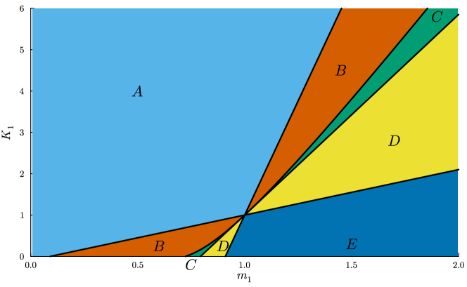
In Figure 1, we fix the parameters inherent to the system as well as $m_{2}$ and $K_{2}$. This is equivalent to having species $x_{2}$ already in the fermentor. We then vary $m_{1}$ and $K_{1}$ to simulate different possible choices of species $x_{1}$. Figure 1 shows the various states in $m_{1}$-$K_{1}$ space. The other constants are $m_{2}=1$, $K_{2}=1$, sin=20superscript๐‘ in20s^{\rm{in}}=20, sยฏ=0.1ยฏ๐‘ 0.1\bar{s}=0.1 and $r=\frac{1}{2}$. Two species can coexist in the central shaded region (C). The point $(1,1)$ corresponds to the case when the two uptake functions are identical and both multipliers are equal to one. The bounding curves of the green shaded region (C) are tangent to one another at this pointย [33].

Refer to caption
Figure 1. Outcomes of two species, $x_{1}$ and $x_{2}$, competing in the fermentor. Parameters sinsuperscript๐‘ ins^{\rm{in}}, sยฏยฏ๐‘ \bar{s}, $m_{2}$ and $K_{2}$ were fixed and parameters $m_{1}$ and $K_{1}$ were varied. A. f2โ€‹(s)>f1โ€‹(s)subscript๐‘“2๐‘ subscript๐‘“1๐‘ f_{2}(s)>f_{1}(s) for sยฏ<s<sยฏ+ยฏ๐‘ ๐‘ superscriptยฏ๐‘ \bar{s}<s<\bar{s}^{+}, so species $x_{2}$ wins the competition. B. The two uptake functions cross, but $x_{2}$ still wins the competition. C. In the green region in the centre, both Floquet multipliers are greater than 1, so, as predicted by Corollaryย 1, both species coexist. D. The uptake functions cross, but $x_{1}$ wins the competition. E. f1โ€‹(s)>f2โ€‹(s)subscript๐‘“1๐‘ subscript๐‘“2๐‘ f_{1}(s)>f_{2}(s) for sยฏ<s<sยฏ+ยฏ๐‘ ๐‘ superscriptยฏ๐‘ \bar{s}<s<\bar{s}^{+}, so $x_{1}$ wins the competition.

4. Three-species competition and simulations

The possibility of survival for two competing species in the self-cycling fermentation process raises the question of whether more species can coexist on a single nonreproducing limiting nutrient. The results in the previous sections cannot easily be applied to competition of $n\geq 3$ species. The impulsive Floquet multipliers can only be calculated with relative ease for systems that can be reduced to two-dimensional systems. However, numerical simulations were run to determine whether three species could coexist.

For the system with three competitors, let $\Lambda_{jk}$ denote the nontrivial Floquet multiplier for the periodic orbit on the boundary $x_{k}=0$, for the system where species $j$ and $k$ are present, but the third species is absent. Then $\Lambda_{kj}$ is the nontrivial Floquet multiplier for the periodic orbit on the boundary $x_{j}=0$, where the third species is absent. We can then apply Theorem 1 to each of the three cases where two species are present and the third species is absent.
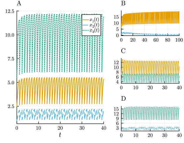
System (2.1) with $n=3$ was simulated using the DifferentialEquations.jl toolbox in Juliaย [26] with sin=20superscript๐‘ in20s^{\rm{in}}=20, sยฏ=0.1ยฏ๐‘ 0.1\bar{s}=0.1, $r=\frac{1}{2}$ and species-specific parameters listed in Table 1.

$j$ $m_{j}$ $K_{j}$ $d_{j}$
1 2.142653 6.33 0.0
2 1.0 1.0 0.0
3 7.0 32.5 0.0
Table 1. Species-specific parameters used in Figure 2. The parameters for Species $x_{1}$ were chosen from Region D in Figure 1, while the parameters for Species $x_{3}$ were chosen from Region C.

Using these data, if $x_{1}$ is absent, we have

$$\Lambda_{23}\ =\ 1.137600,\qquad\Lambda_{32}\ =\ 1.049998.$$

Thus, in the absence of $x_{1}$, we see that $x_{2}$ and $x_{3}$ persist by Theorem 1. If $x_{2}$ is absent, we have

$$\Lambda_{13}\ =\ 1.008808,\qquad\Lambda_{31}\ =\ 1.014487.$$

Thus, in the absence of $x_{2}$, we see that $x_{1}$ and $x_{3}$ persist by Theorem 1. If $x_{3}$ is absent, we have

$$\Lambda_{12}\ =\ 0.985852,\qquad\Lambda_{21}\ =\ 1.089587.$$

Thus, in the absence of $x_{3}$, we find that $x_{1}$ and $x_{2}$ cannot coexist. It follows that this system is an example of competitor-mediated coexistence, since $x_{2}$ cannot survive in the presence of $x_{1}$ unless $x_{3}$ is also present.

Refer to caption
Figure 2. A. Three microorganisms competing for a single resource in the self-cycling fermentor. The species appear to be persisting over time, suggesting coexistence. Note in particular that $x_{2}$ is the weakest competitor. B. Species $x_{2}$ cannot survive in the presence of $x_{1}$ if $x_{3}$ is absent, demonstrating competitor-mediated coexistence. C. Species $x_{1}$ and $x_{3}$ coexist. D. Species $x_{2}$ and $x_{3}$ coexist.

5. Discussion

Coexistence of more than one species is possible in the self-cycling fermentation process. The model with only two species is simple enough that we are able to prove when two species are able to survive in the same environment using impulsive Floquet theory. However, we are not able to determine the exact form of that coexistence in a general setting. In the special case where the decay rates of both species are negligible, we are able to reduce the dynamics to those of a one-dimensional monotone dynamical system. The general theory of monotone dynamical systems allows us to conclude that coexistence is in the form of a periodic solution with one impulse per period.

In the analogous model of the chemostat, where the nutrient is pumped in continuously at a constant rate, coexistence of two species competing for a single nonreproducing nutrient is not possible (aside from a few knife-edge cases involving the equality of certain parameters)ย [32, 40]. The results here are similar to competition in the chemostat with periodic dilution rateย [41]. There, multiple species are able to coexist provided that each species is the best competitor for a significant portion of the dilution cycle. A similar condition was required for the coexistence of two species in a model of serial transfer culturesย [31]. Here, we have extended those results to competition in the self-cycling fermentation process. If one species is the best competitor at every nutrient concentration, then that species will out-compete the others. However, while being a better competitor at some nutrient levels is necessary for survival, it is not sufficient.

We were unable to find analogous theoretical results to determine the outcome of three-species competition. However, numerical simulations show that coexistence between three species is possible. Interestingly, two of the species in our example are unable to coexist without the third species present. This phenomenon of competitor-mediated coexistence has also been observed in other resource-competition modelsย [1].

In applications where the system is best served by a particular class of microorganism, we give conditions for the exclusion of other competing species or strains. Our results suggest that it may be possible to tune reactor parameters, such as the decanting fraction $r$ and decanting criterion sยฏยฏ๐‘ \bar{s}, in order to exclude unwanted competitors. This could be an important strategy used to maintain desired populations in wastewater treatment systemsย [18, 29, 37].

For applications in which the goal is to maximize the throughput of the system โ€” as would be the case in the production of polyhydroxyalkanoates โ€” having multiple species present may provide a more robust system. The coexistence of multiple species offers a buffer in the event that one species abruptly dies off. It is unclear whether the production efficiency would be increased or decreased by the presence of more species, although experimental evidence suggests that an increase is possibleย [16]. The fact that three species can co-exist in the self-cycling fermentor suggests the possibility of multiple species co-existing simultaneously under appropriate conditions. This has implications for more efficient treatment of wastewater and greater yield, with a buffer against unexpected species extinction.

References

  • [1] J.ย Arino, S.S. Pilyugin, and G.S.K. Wolkowicz. Considerations on yield, nutrient uptake, cellular growth, and competition in chemostat models. Canadian Applied Mathematics Quarterly, 11(2):107โ€“142, 2003.
  • [2] D.D. Bainov and P.S. Simeonov. Systems with Impulsive Effect. Ellis Horwood Ltd, Chichester, 1989.
  • [3] D.D. Bainov and P.S. Simeonov. Impulsive differential equations: periodic solutions and applications. Longman Scientific and Technical, Burnt Mill, 1993.
  • [4] D.G.ย Cooper B.M.ย Wincure and A.ย Rey. Mathematical model of self-cycling fermentation. Journal of Biotechnology and Bioengineering, 46:180โ€“183, 1995.
  • [5] W.A. Brown and D.G. Cooper. Self-cycling fermentation applied to acinetobacter calcoaceticus. Applied and Environmental Microbiology, 57(10):2901โ€“2906, 1991.
  • [6] A.ย Dutta and S.ย Sarkar. Sequencing batch reactor for wastewater treatment: recent advances. Current Pollution Reports, 1:177โ€“190, 2015.
  • [7] G.ย Fan and G.S.K. Wolkowicz. Analysis of a model of nutrient driven self-cycling fermentation allowing unimodal response functions. Discrete and Continuous Dynamical Systems-B, 8(4):801โ€“831, 2007.
  • [8] H.I. Freedman and J.W.-H. So. Persistence in discrete semidynamical systems. SIAM Journal of Mathematical Analysis, 20(4):930โ€“938, 1989.
  • [9] B.H. Good, M.J. McDonald, J.E. Barrick, R.E. Lenski, and M.M. Desai. The dynamics of molecular evolution over 60,000 generations. Nature, 551(7678):45โ€“50, 2017.
  • [10] S.R. Hansen and S.P. Hubbell. Single-nutrient microbial competition: qualitative agreement between experimental and theoretically forecast outcomes. Science, 207(4438):1491โ€“1493, 1980.
  • [11] M.W. Hirsch and H.L. Smith. Monotone dynamical systems. Handbook of differential equations: ordinary differential equations, 2:239โ€“357, 2006.
  • [12] J.N. Housby and N.H. Mann. Phage therapy. Drug discovery today, 14(11-12):536โ€“540, 2009.
  • [13] T.-H. Hsu, T.ย Meadows, G.S.K. Wolkowicz, and L.ย Wang. Growth on two limiting essential resources in a self-cycling fermentor. Mathematical Biosciences and Engineering, 16(1):78โ€“100, 2019.
  • [14] S.M. Hughes and D.G. Cooper. Biodegredation of phenol using the self-cycling fermentation (scf) process. Journal of Biotechnology and Bioengineering, 51:112โ€“119, 1996.
  • [15] C.ย Kocharunchitt, T.ย Ross, and D.L. McNeil. Use of bacteriophages as biocontrol agents to control salmonella associated with seed sprouts. International journal of food microbiology, 128(3):453โ€“459, 2009.
  • [16] C.N.L.K. Kourmentza, I.ย Ntaikou, G.ย Lyberatos, and M.ย Kornaros. Polyhydroxyalkanoates from pseudomonas sp. using synthetic and olive mill wastewater under limiting conditions. International journal of biological macromolecules, 74:202โ€“210, 2015.
  • [17] S.ย Liu, X.ย Wang, L.ย Wang, and H.ย Song. Competitive exclusion in delayed chemostat models with differential removal rates. SIAM Journal on Applied Mathematics, 74(3):634โ€“648, 2014.
  • [18] C.M Lopez-Vazquez, A.ย Oehmen, C.M. Hooijmans, D.ย Brdjanovic, H.J Gijzen, Z.ย Yuan, and M.C.M. van Loosdrecht. Modeling the paoโ€“gao competition: effects of carbon source, ph and temperature. Water Research, 43(2):450โ€“462, 2009.
  • [19] T.ย Meadows and G.S.K. Wolkowicz. Growth on multiple interactive-essential resources in a self-cycling fermentor: An impulsive differential equations approach. Nonlinear Analysis: Real World Applications, 56:103157, 2020.
  • [20] R.K. Miller and A.N. Michel. Ordinary Differential Equations. Academic Press, Inc., Orlando, 1982.
  • [21] H.L.ย Smith M.W.ย Hirsch and X.-Q. Zhao. Chain transitivity, attractivity and strong repellors for semidynamical systems. Journal of Dynamics and Differential Equations, 13:101โ€“131, 2001.
  • [22] A.-L. Nguyen, S.J.B. Duff, and J.D. Sheppard. Application of feedback control based on dissolved oxygen to a fixed-film sequencing batch reactor for treatment of brewery wastewater. Water environment research, 72(1):75โ€“83, 2000.
  • [23] T.ย Nguyenhuynh, L.W. Yoon, Y.H. Chow, and A.S.M. Chua. An insight into enrichment strategies for mixed culture in polyhydroxyalkanoate production: feedstocks, operating conditions and inherent challenges. Chemical Engineering Journal, 420:130488, 2021.
  • [24] J.S. Oh, S.S. Choi, J.-K. Yeo, and T.H. Park. Construction of various bacteriophage $\lambda$ mutants for stable and efficient production of recombinant protein in escherichia coli. Process Biochemistry, 42(3):486โ€“490, 2007.
  • [25] A.ย Pervez, P.P. Singh, and H.ย BozdoฤŸan. Ecological perspective of the diversity of functional responses. European Journal of Environmental Sciences, 8(2):97โ€“101, 2018.
  • [26] C.ย Rackauckas and Q.ย Nie. DifferentialEquations.jlโ€“a performant and feature-rich ecosystem for solving differential equations in Julia. Journal of Open Research Software, 5(1), 2017.
  • [27] B.E. Sarkis and D.G. Cooper. Biodegradation of aromatic compounds in a self-cycling fermenter (scf). The Canadian Journal of Chemical Engineering, 72:874โ€“880, 1994.
  • [28] D.ย Sauvageau and D.G. Cooper. Two-stage, self-cycling process for the production of bacteriophages. Microbial Cell Factories, 9:1โ€“10, 2010.
  • [29] N.ย Shen and Y.ย Zhou. Enhanced biological phosphorus removal with different carbon sources. Applied microbiology and biotechnology, 100:4735โ€“4745, 2016.
  • [30] J.D. Sheppard and D.G. Cooper. Development of computerized feedback control for the continuous phasing of bacillus subtilis. Biotechnology and bioengineering, 36(5):539โ€“545, 1990.
  • [31] H.L. Smith. Bacterial competition in serial transfer culture. Mathematical biosciences, 229(2):149โ€“159, 2011.
  • [32] H.L. Smith and P.ย Waltman. The Theory of the Chemostat: Dynamics of Microbial Competition. Cambridge University Press, New York, 1995.
  • [33] R.ย Smith. Impulsive differential equations with applications to self-cycling fermentation. PhD thesis, 2001.
  • [34] R.J. Smith and G.S.K. Wolkowicz. A size-structured model for the nutrient-driven self-cycling fermentation process. Dynamics of Continuous, Discrete and Impulsive Systems, 10:207โ€“219, 2003.
  • [35] R.J. Smith and G.S.K. Wolkowicz. Analysis of a model of the nutrient driven self-cycling fermentation process. Dynamics of Continuous Discrete and Impulsive Systems Series B, 11:239โ€“266, 2004.
  • [36] Y.ย Tan, R.V.C. Agustin, L.Y. Stein, and D.ย Sauvageau. Transcriptomic analysis of synchrony and productivity in self-cycling fermentation of engineered yeast producing shikimic acid. Biotechnology Reports, 32:e00691, 2021.
  • [37] H.P. Trinh, S.-H. Lee, G.ย Jeong, H.ย Yoon, and H.-D. Park. Recent developments of the mainstream anammox processes: challenges and opportunities. Journal of Environmental Chemical Engineering, 9(4):105583, 2021.
  • [38] J.ย Wang, M.ย Chae, D.ย Beyene, D.ย Sauvageau, and D.C. Bressler. Co-production of ethanol and cellulose nanocrystals through self-cycling fermentation of wood pulp hydrolysate. Bioresource Technology, 330:124969, 2021.
  • [39] J.ย Wang, M.ย Chae, D.C. Bressler, and D.ย Sauvageau. Improved bioethanol productivity through gas flow rate-driven self-cycling fermentation. Biotechnology for biofuels, 13:1โ€“14, 2020.
  • [40] G.S.K. Wolkowicz and Z.ย Lu. Global dynamics of a mathematical model of competition in the chemostat: general response functions and differential death rates. SIAM Journal on Applied Mathematics, 52(1):222โ€“233, 1992.
  • [41] G.S.K. Wolkowicz and X.-Q. Zhao. N-species competition in a periodic chemostat. Differential and Integral Equations, 11(3):465โ€“491, 1998.

Appendix A Proofs

Proof of Proposition 1.

That sโ€‹(t)๐‘ ๐‘กs(t) remains nonnegative is obvious. The faces of $\mathbb{R}^{1+n}_{+}$ with $x_{j}=0$ are invariant under (2.1a), and therefore, by the uniqueness of solutions to ODEs, the interior of $\mathbb{R}_{+}^{n+1}$ is invariant. Since impulses take $x_{j}(t)$ to $(1-r)x_{j}(t)$, if $x_{j}(0)>0$, then $x_{j}(t)>0$ for all $t$.

Next we show that solutions with the given initial conditions reach sโ€‹(t)=sยฏ๐‘ ๐‘กยฏ๐‘ s(t)=\bar{s} in finite time. Suppose not. Then there exists sโˆ—>sยฏsuperscript๐‘ ยฏ๐‘ s^{*}>\bar{s} such that as $t\to\infty$, sโ€‹(t)โ†’sโˆ—โ†’๐‘ ๐‘กsuperscript๐‘ s(t)\to s^{*} and $x_{j}(t)\to 0$ for each $j\in\{1,...,n\}$. If $u(t)=\sum_{j=1}^{n}x_{j}(t)$, then

dโ€‹udโ€‹s=โˆ‘j=1n(fjโ€‹(s)โˆ’dj)โ€‹xjโˆ’โˆ‘j=1nfjโ€‹(s)โ€‹xj.๐‘‘๐‘ข๐‘‘๐‘ superscriptsubscript๐‘—1๐‘›subscript๐‘“๐‘—๐‘ subscript๐‘‘๐‘—subscript๐‘ฅ๐‘—superscriptsubscript๐‘—1๐‘›subscript๐‘“๐‘—๐‘ subscript๐‘ฅ๐‘—\frac{du}{ds}=\frac{\sum_{j=1}^{n}(f_{j}(s)-d_{j})x_{j}}{-\sum_{j=1}^{n}f_{j}(s)x_{j}}.

Integrating with respect to s๐‘ s gives

uโ€‹(s)โˆ’uโ€‹(sยฏ+)=โˆซssยฏ+โˆ‘j=1n(fjโ€‹(ฯƒ)โˆ’dj)โ€‹xjโ€‹(ฯƒ)โˆ‘j=1nfjโ€‹(ฯƒ)โ€‹xjโ€‹(ฯƒ)โ€‹๐‘‘ฯƒ.๐‘ข๐‘ ๐‘ขsuperscriptยฏ๐‘ superscriptsubscript๐‘ superscriptยฏ๐‘ superscriptsubscript๐‘—1๐‘›subscript๐‘“๐‘—๐œŽsubscript๐‘‘๐‘—subscript๐‘ฅ๐‘—๐œŽsuperscriptsubscript๐‘—1๐‘›subscript๐‘“๐‘—๐œŽsubscript๐‘ฅ๐‘—๐œŽdifferential-d๐œŽu(s)-u(\bar{s}^{+})=\int_{s}^{\bar{s}^{+}}\frac{\sum_{j=1}^{n}(f_{j}(\sigma)-d_{j})x_{j}(\sigma)}{\sum_{j=1}^{n}f_{j}(\sigma)x_{j}(\sigma)}d\sigma.

If sโˆ—โ‰ฅฮปmโ€‹aโ€‹xsuperscript๐‘ subscript๐œ†๐‘š๐‘Ž๐‘ฅs^{*}\geq\lambda_{max}, then the integrand is positive for all sโˆ—<s<sยฏ+superscript๐‘ ๐‘ superscriptยฏ๐‘ s^{*}<s<\bar{s}^{+}. This implies that

0>โˆ’uโ€‹(sยฏ+)=โˆซsโˆ—sยฏ+โˆ‘j=1n(fjโ€‹(ฯƒ)โˆ’dj)โ€‹xjโ€‹(ฯƒ)โˆ‘j=1nfjโ€‹(ฯƒ)โ€‹xjโ€‹(ฯƒ)โ€‹๐‘‘ฯƒ>0,0๐‘ขsuperscriptยฏ๐‘ superscriptsubscriptsuperscript๐‘ superscriptยฏ๐‘ superscriptsubscript๐‘—1๐‘›subscript๐‘“๐‘—๐œŽsubscript๐‘‘๐‘—subscript๐‘ฅ๐‘—๐œŽsuperscriptsubscript๐‘—1๐‘›subscript๐‘“๐‘—๐œŽsubscript๐‘ฅ๐‘—๐œŽdifferential-d๐œŽ00>-u(\bar{s}^{+})=\int_{s^{*}}^{\bar{s}^{+}}\frac{\sum_{j=1}^{n}(f_{j}(\sigma)-d_{j})x_{j}(\sigma)}{\sum_{j=1}^{n}f_{j}(\sigma)x_{j}(\sigma)}d\sigma>0,

yielding a contradiction. If sยฏโ‰คsโˆ—<ฮปmโ€‹aโ€‹x,ยฏ๐‘ superscript๐‘ subscript๐œ†๐‘š๐‘Ž๐‘ฅ\overline{s}\leq s^{*}<\lambda_{max}, then

โˆ’uโ€‹(sยฏ+)๐‘ขsuperscriptยฏ๐‘ \displaystyle-u(\bar{s}^{+}) =โˆซsโˆ—sยฏ+โˆ‘j=1n(fjโ€‹(ฯƒ)โˆ’dj)โ€‹xjโ€‹(ฯƒ)โˆ‘j=1nfjโ€‹(ฯƒ)โ€‹xjโ€‹(ฯƒ)โ€‹๐‘‘ฯƒabsentsuperscriptsubscriptsuperscript๐‘ superscriptยฏ๐‘ superscriptsubscript๐‘—1๐‘›subscript๐‘“๐‘—๐œŽsubscript๐‘‘๐‘—subscript๐‘ฅ๐‘—๐œŽsuperscriptsubscript๐‘—1๐‘›subscript๐‘“๐‘—๐œŽsubscript๐‘ฅ๐‘—๐œŽdifferential-d๐œŽ\displaystyle=\int_{s^{*}}^{\bar{s}^{+}}\frac{\sum_{j=1}^{n}(f_{j}(\sigma)-d_{j})x_{j}(\sigma)}{\sum_{j=1}^{n}f_{j}(\sigma)x_{j}(\sigma)}d\sigma
โ‰ฅโˆซsโˆ—ฮปmโ€‹aโ€‹xminjโก(fjโ€‹(ฯƒ)โˆ’dj)minjโก(fjโ€‹(ฯƒ))โ€‹๐‘‘ฯƒ+โˆซฮปmโ€‹aโ€‹xsยฏ+minjโก(fjโ€‹(ฯƒ)โˆ’dj)maxjโก(fjโ€‹(ฯƒ))โ€‹๐‘‘ฯƒabsentsuperscriptsubscriptsuperscript๐‘ subscript๐œ†๐‘š๐‘Ž๐‘ฅsubscript๐‘—subscript๐‘“๐‘—๐œŽsubscript๐‘‘๐‘—subscript๐‘—subscript๐‘“๐‘—๐œŽdifferential-d๐œŽsuperscriptsubscriptsubscript๐œ†๐‘š๐‘Ž๐‘ฅsuperscriptยฏ๐‘ subscript๐‘—subscript๐‘“๐‘—๐œŽsubscript๐‘‘๐‘—subscript๐‘—subscript๐‘“๐‘—๐œŽdifferential-d๐œŽ\displaystyle\geq\int_{s^{*}}^{\lambda_{max}}\frac{\min_{j}(f_{j}(\sigma)-d_{j})}{\min_{j}(f_{j}(\sigma))}d\sigma+\int_{\lambda_{max}}^{\bar{s}^{+}}\frac{\min_{j}(f_{j}(\sigma)-d_{j})}{\max_{j}(f_{j}(\sigma))}d\sigma
$\displaystyle\geq\mu_{min},$

where the last inequality follows since the integrand of the first integral is negative on the domain of integration. Therefore sยฏยฏ๐‘ \bar{s} is reached in finite time and an impulse occurs.

The solution is then reset so that s=(1โˆ’r)โ€‹sยฏ+rโ€‹sin>sยฏ๐‘ 1๐‘Ÿยฏ๐‘ ๐‘Ÿsuperscript๐‘ inยฏ๐‘ s=(1-r)\bar{s}+rs^{\rm{in}}>\bar{s} (since sin>sยฏsuperscript๐‘ inยฏ๐‘ s^{\rm{in}}>\bar{s}), and the sum of the $x_{j}$โ€™s remain positive. Therefore, the original assumptions on the initial conditions are once again satisfied. Hence, solutions cycle indefinitely. โˆŽ

Lemma 2.

The function $\varphi=\varphi(t,\tau,\xi)$ that solves (2.1a) for $n=2$ with initial condition $\varphi(\tau,\tau,\xi)=\xi$ is continuous in $(t,\tau,\xi)$.

Proof.

We have

(sโ€ฒx1โ€ฒx2โ€ฒ)=(โˆ’f1โ€‹(s)โ€‹x1โˆ’f2โ€‹(s)โ€‹x2x1โ€‹(f1โ€‹(s)โˆ’d1)x2โ€‹(f2โ€‹(s)โˆ’d2))=Fโ€‹(t,w)superscript๐‘ โ€ฒsuperscriptsubscript๐‘ฅ1โ€ฒsuperscriptsubscript๐‘ฅ2โ€ฒsubscript๐‘“1๐‘ subscript๐‘ฅ1subscript๐‘“2๐‘ subscript๐‘ฅ2subscript๐‘ฅ1subscript๐‘“1๐‘ subscript๐‘‘1subscript๐‘ฅ2subscript๐‘“2๐‘ subscript๐‘‘2๐น๐‘ก๐‘ค\displaystyle\left(\begin{array}[]{c}s^{\prime}\\ x_{1}^{\prime}\\ x_{2}^{\prime}\end{array}\right)=\left(\begin{array}[]{c}-f_{1}(s)x_{1}-f_{2}(s)x_{2}\\ x_{1}(f_{1}(s)-d_{1})\\ x_{2}(f_{2}(s)-d_{2})\end{array}\right)\ =\ F(t,w)

where w=(s,x1,x2)๐‘ค๐‘ subscript๐‘ฅ1subscript๐‘ฅ2w=(s,x_{1},x_{2}). Then

Fw=[โˆ’f1โ€ฒโ€‹(s)โ€‹x1โˆ’f2โ€ฒโ€‹(s)โ€‹x2โˆ’f1โ€‹(s)โˆ’f2โ€‹(s)x1โ€‹f1โ€ฒโ€‹(s)f1โ€‹(s)โˆ’d10x2โ€‹f2โ€ฒโ€‹(s)0f2โ€‹(s)โˆ’d2]subscript๐น๐‘คdelimited-[]superscriptsubscript๐‘“1โ€ฒ๐‘ subscript๐‘ฅ1superscriptsubscript๐‘“2โ€ฒ๐‘ subscript๐‘ฅ2subscript๐‘“1๐‘ subscript๐‘“2๐‘ subscript๐‘ฅ1superscriptsubscript๐‘“1โ€ฒ๐‘ subscript๐‘“1๐‘ subscript๐‘‘10subscript๐‘ฅ2superscriptsubscript๐‘“2โ€ฒ๐‘ 0subscript๐‘“2๐‘ subscript๐‘‘2\displaystyle F_{w}=\left[\begin{array}[]{ccc}-f_{1}^{\prime}(s)x_{1}-f_{2}^{\prime}(s)x_{2}&-f_{1}(s)&-f_{2}(s)\\ x_{1}f_{1}^{\prime}(s)&f_{1}(s)-d_{1}&0\\ x_{2}f_{2}^{\prime}(s)&0&f_{2}(s)-d_{2}\end{array}\right]

Each function $f_{i}$, $j=1,2$ is continuously differentiable, so $F$ and $F_{w}$ are continuous. Hence $\phi(t,\tau,\xi)$ is continuous in $(t,\tau,\xi)$ by Theorem 7.1 inย [20]. โˆŽ

Proof of Theorem 1.

Consider any initial point (sยฏ+,x1โ€‹(0),x2โ€‹(0))superscriptยฏ๐‘ subscript๐‘ฅ10subscript๐‘ฅ20(\bar{s}^{+},x_{1}(0),x_{2}(0)) where $x_{1}(0)>0$ and $x_{2}(0)>0$. By Proposition 1, there exists a first time $t_{1}$ such that solutions of (2.1) satisfy

sโ€‹(t1โˆ’)=sยฏ,x1โ€‹(t1โˆ’)> 0,x2โ€‹(t1โˆ’)> 0.formulae-sequence๐‘ superscriptsubscript๐‘ก1ยฏ๐‘ formulae-sequencesubscript๐‘ฅ1superscriptsubscript๐‘ก1 0subscript๐‘ฅ2superscriptsubscript๐‘ก1 0s(t_{1}^{-})\ =\ \bar{s},\quad x_{1}(t_{1}^{-})\ >\ 0,\quad x_{2}(t_{1}^{-})\ >\ 0.

Then if $t_{n}$ denotes the time of the $n$th impulse point, we have, for $t_{n-1}<t<t_{n}$ ($n>1$),

0<sยฏ<sโ€‹(t)<sยฏ+0ยฏ๐‘ ๐‘ ๐‘กsuperscriptยฏ๐‘ \displaystyle 0<\bar{s}<s(t)<\bar{s}^{+}

and, for each $j\in\{1,2\}$, either

$$0<(1-r)x_{j}(t_{n-1}^{-})<x_{j}(t)\quad\text{or}\quad 0<x_{j}(t_{n}^{-})<x_{j}(t).$$

Therefore, it suffices to consider the sequence $\{(u_{n},v_{n})\}_{n=1}^{\infty}$ where $u_{n}=x_{1}(t_{n}^{-})$ and $v_{n}=x_{2}(t_{n}^{-})$ and to show that

$$\liminf_{n\rightarrow\infty}u_{n}\ >\ 0\quad\mbox{and}\quad\liminf_{n\rightarrow\infty}v_{n}\ >\ 0.$$

The equilibrium point (sยฏ,0,0)ยฏ๐‘ 00(\bar{s},0,0) of system (2.1) is unstable with a one-dimensional centre manifold along the s๐‘ s-axis and a two-dimensional unstable manifold that intersects the plane

Ssยฏ={(s,x1,x2):s=sยฏ,x1โ‰ฅ0,x2โ‰ฅ0}subscript๐‘†ยฏ๐‘ conditional-set๐‘ subscript๐‘ฅ1subscript๐‘ฅ2formulae-sequence๐‘ ยฏ๐‘ formulae-sequencesubscript๐‘ฅ10subscript๐‘ฅ20\displaystyle S_{\bar{s}}=\left\{(s,x_{1},x_{2}):s=\bar{s},x_{1}\geq 0,x_{2}\geq 0\right\}

along a smooth curve, say $g(x_{1},x_{2})=0$. This curve in $\mathbb{R}^{2}_{+}$ connecting the boundary points $(\hat{x}_{1},0)$ and $(0,\hat{x}_{2})$, where $\hat{x}_{1}>0$ and $\hat{x}_{2}>0$, divides the plane Ssยฏsubscript๐‘†ยฏ๐‘ S_{\bar{s}} into a bounded region and an unbounded region. Without loss of generality, assume

$$X=\{(x_{1},x_{2}):x_{1}\geq 0,x_{2}\geq 0,g(x_{1},x_{2})\geq 0\}$$

denotes the unbounded region.

Define the map $f:X\rightarrow X$ in the following way:

$$f(u_{n},v_{n})=(u_{n+1},v_{n+1}),$$

where we set sโ€‹(0)=sยฏ+,x1โ€‹(0)=un+,x2โ€‹(0)=vn+formulae-sequence๐‘ 0superscriptยฏ๐‘ formulae-sequencesubscript๐‘ฅ10superscriptsubscript๐‘ข๐‘›subscript๐‘ฅ20superscriptsubscript๐‘ฃ๐‘›s(0)=\bar{s}^{+},\ x_{1}(0)=u_{n}^{+},\ x_{2}(0)=v_{n}^{+} and then determine $u_{n+1}=x_{1}(t_{1}^{-})$ and $v_{n+1}=x_{2}(t_{1}^{-})$ from system (2.1).

Note that for any initial condition of the form sโ€‹(0)=sยฏ+๐‘ 0superscriptยฏ๐‘ s(0)=\bar{s}^{+}, $x_{1}(0)>0$ and $x_{2}(0)>0$, we have sโ€‹(t1โˆ’)=sยฏ๐‘ superscriptsubscript๐‘ก1ยฏ๐‘ s(t_{1}^{-})=\bar{s}, $x_{1}(t_{1}^{-})>0$ and $x_{2}(t_{1}^{-})>0$, so sโ€‹(t1+)=sยฏ+๐‘ superscriptsubscript๐‘ก1superscriptยฏ๐‘ s(t_{1}^{+})=\bar{s}^{+}, $x_{1}(t_{1}^{+})>0$ and $x_{2}(t_{1}^{+})>0$ and then sโ€‹(t2โˆ’)=sยฏ๐‘ superscriptsubscript๐‘ก2ยฏ๐‘ s(t_{2}^{-})=\bar{s} and $g(x_{1}(t_{2}^{-}),x_{2}(t_{2}^{-}))>0$. It follows that $f(X)\subset X$.

Next we show that $f$ is continuous on $X$ by showing that $f$ is a composition $p\circ q:X\rightarrow X$ of two continuous functions,

$$q:X\rightarrow X\qquad\mbox{and}\qquad p:X\rightarrow X.$$

Define

$\displaystyle q(x_{1},x_{2})$ $\displaystyle=\left((1-r)x_{1},(1-r)x_{2}\right)$

and

$\displaystyle p(x_{1},x_{2})$ $\displaystyle=(u(x_{1},x_{2}),v(x_{1},x_{2})),$

where $u(x_{1},x_{2})=x_{1}(\bar{t})$ and $v(x_{1},x_{2})=x_{2}(\bar{t})$ such that (sโ€‹(t),x1โ€‹(t),x2โ€‹(t))๐‘ ๐‘กsubscript๐‘ฅ1๐‘กsubscript๐‘ฅ2๐‘ก(s(t),x_{1}(t),x_{2}(t)), $0\leq t\leq\bar{t}$ is the solution of the associated ODE (2.1a) with initial conditions

sโ€‹(0)=sยฏ+,x1โ€‹(0)=x1,x2โ€‹(0)=x2formulae-sequence๐‘ 0superscriptยฏ๐‘ formulae-sequencesubscript๐‘ฅ10subscript๐‘ฅ1subscript๐‘ฅ20subscript๐‘ฅ2s(0)=\bar{s}^{+},\quad x_{1}(0)=x_{1},\quad x_{2}(0)=x_{2}

and sยฏ<sโ€‹(t)<(1โˆ’r)โ€‹sยฏ+rโ€‹sinยฏ๐‘ ๐‘ ๐‘ก1๐‘Ÿยฏ๐‘ ๐‘Ÿsuperscript๐‘ in\bar{s}<s(t)<(1-r)\bar{s}+rs^{\rm{in}} for $0<t<\bar{t}$ and sโ€‹(tยฏ)=sยฏ๐‘ ยฏ๐‘กยฏ๐‘ s(\bar{t})=\bar{s}.

It is clear that $q$ is continuous. That $p$ is continuous follows from continuous dependence on initial data for ordinary differential equations (see Lemma 2).

The map $f$ has two equilibrium points, $P_{1}=(\bar{x}_{1},0)$ and $P_{2}=(0,\bar{x}_{2})$, where $\bar{x}_{j}>0$, $j=1,2$. $P_{1}$ and $P_{2}$ represent single species survival equilibria of the map and correspond to the nontrivial periodic orbits on the s๐‘ s-$x_{1}$ and s๐‘ s-$x_{2}$ planes, respectively, of system (2.1). Each $P_{j}$, $j=1,2$, is clearly an isolated invariant set.

Assume that $(x_{1}(t_{1}),x_{2}(t_{1}))$ is any point in $X$ that satisfies $x_{1}(t_{1})>0$ and $x_{2}(t_{1})>0$. Consider the compact positive orbit $\left\{x_{1}(t_{n}),x_{2}(t_{n})\right\}_{n\in\mathbb{Z}_{+}}$ generated by the map $f$. Assume also that

$$\liminf_{n\rightarrow\infty}x_{1}(t_{n})=0\quad\mbox{or}\quad\liminf_{n\rightarrow\infty}x_{2}(t_{n})=0.$$

Then either

  1. (a)

    there is a subsequence such that

    $$\lim_{k\rightarrow\infty}x_{1}(t_{n_{k}})=0\quad\mbox{and}\quad\lim_{k\rightarrow\infty}x_{2}(t_{n_{k}})>0,\qquad\mbox{or}$$
  2. (b)

    there is a subsequence such that

    $$\lim_{k\rightarrow\infty}x_{1}(t_{n_{k}})>0\quad\mbox{and}\quad\lim_{k\rightarrow\infty}x_{2}(t_{n_{k}})=0.$$

In case (a), we must have

$\displaystyle P_{2}\in\omega\left(\left\{x_{1}(t_{n}),x_{2}(t_{n})\right\}_{n\in\mathbb{Z}_{+}}\right).$

However, since $\Lambda_{21}>1$, the stable manifold of $P_{2}$ is the set

$\displaystyle W^{+}(P_{2})=\{(x_{1},x_{2}):x_{1}=0,x_{2}>0\}.$

Since $x_{1}(t_{n_{k}})>0$ for all $k$,

$\displaystyle\left\{x_{1}(t_{n}),x_{2}(t_{n})\right\}_{n\in\mathbb{Z}_{+}}\subseteq W^{+}_{\mbox{w}}(P_{2})\backslash W^{+}(P_{2}).$

Hence, by Theorem 3.1 ofย [8], there exists a positive orbit $\left\{a(t_{n}),b(t_{n})\right\}_{n\in\mathbb{Z}_{+}}$ in

$$\omega\left(\left\{x_{1}(t_{n}),x_{2}(t_{n})\right\}_{n\in\mathbb{Z}_{+}}\right)$$

such that (aโ€‹(t1),bโ€‹(t1))โ‰ P2๐‘Žsubscript๐‘ก1๐‘subscript๐‘ก1subscript๐‘ƒ2(a(t_{1}),b(t_{1}))\neq P_{2} and

$$\left\{a(t_{n}),b(t_{n})\right\}_{n\in\mathbb{Z}_{+}}\subseteq W^{+}(P_{2}).$$

Hence $a(t_{n})=0$ for all $n$. It follows that the omega limit set of $\left\{x_{1}(t_{n}),x_{2}(t_{n})\right\}_{n\in\mathbb{Z}_{+}}$ is a subset of $W^{+}(P_{2})$.

The orbit $\left\{x_{1}(t_{n}),x_{2}(t_{n})\right\}_{n\in\mathbb{Z}_{+}}$ is a pseudo-asymptotic orbit of $f$, so by Lemma 2.3 inย [21] the omega limit set is nonempty, compact and invariant. This set cannot include the portion of the $x_{2}$ axis above $P_{2}$, since it is unbounded.

Consider the set

$$M=\left\{(0,x_{2}):\hat{x}_{2}\leq x_{2}\leq\bar{x}_{2}\right\}.$$

Clearly $f(M)\subset M$, but $M\not\subset f(M)$, since $f$ is a non-decreasing map on $M$ and $f(0,\hat{x}_{2})=(0,y)$ where $y>\hat{x}_{2}$. Thus $M$ is not an invariant set.

The only other invariant set in $W^{+}(P_{2})$ is $P_{2}$ itself. Thus

$\displaystyle\omega\left(\left\{x_{1}(t_{n}),x_{2}(t_{n})\right\}_{n\in\mathbb{Z}_{+}}\right)=P_{2}.$

However, this implies that

$$\left\{x_{1}(t_{n}),x_{2}(t_{n})\right\}_{n\in\mathbb{Z}_{+}}\subset W^{+}(P_{2}),$$

which is a contradiction. Thus case (a) is impossible.

Case (b) can be ruled out in a similar fashion.

Hence, for any point $(x_{1}(t_{1}),x_{2}(t_{1}))$ with $x_{1}(t_{1})>0$, $x_{2}(t_{1})>0$, we have

$$\liminf_{n\rightarrow\infty}x_{1}(t_{n})>0\qquad\mbox{and}\qquad\liminf_{n\rightarrow\infty}x_{2}(t_{n})>0.$$

โˆŽ

Proof of Lemma 1.

Assume that $d_{j}=0,\ i=1,...n.$ Then, adding together all the equations in (2.1), it follows that between impulses (s+โˆ‘j=1nxj)โ€ฒโ€‹(t)=0.superscript๐‘ superscriptsubscript๐‘—1๐‘›subscript๐‘ฅ๐‘—โ€ฒ๐‘ก0\left(s+\sum_{j=1}^{n}x_{j}\right)^{\prime}(t)=0. Therefore, for each $k\in\mathbb{N}$, we can define a constant $c_{k}$ such that

sโ€‹(t)+โˆ‘j=1nxjโ€‹(t)๐‘ ๐‘กsuperscriptsubscript๐‘—1๐‘›subscript๐‘ฅ๐‘—๐‘ก\displaystyle s(t)+\sum_{j=1}^{n}x_{j}(t) $\displaystyle=c_{k}$

for $t_{k}<t<t_{k+1}.$ At the moments of impulse, we have

$\displaystyle c_{k+1}$ =sโ€‹(tk+1+)+โˆ‘j=1nxjโ€‹(tk+1+)absent๐‘ superscriptsubscript๐‘ก๐‘˜1superscriptsubscript๐‘—1๐‘›subscript๐‘ฅ๐‘—superscriptsubscript๐‘ก๐‘˜1\displaystyle=s(t_{k+1}^{+})+\sum_{j=1}^{n}x_{j}(t_{k+1}^{+})
=rโ€‹sin+(1โˆ’r)โ€‹sโ€‹(tk+1โˆ’)+(1โˆ’r)โ€‹โˆ‘j=1nxjโ€‹(tk+1โˆ’)absent๐‘Ÿsuperscript๐‘ in1๐‘Ÿ๐‘ superscriptsubscript๐‘ก๐‘˜11๐‘Ÿsuperscriptsubscript๐‘—1๐‘›subscript๐‘ฅ๐‘—superscriptsubscript๐‘ก๐‘˜1\displaystyle=rs^{\rm{in}}+(1-r)s(t_{k+1}^{-})+(1-r)\sum_{j=1}^{n}x_{j}(t_{k+1}^{-})
=rโ€‹sin+(1โˆ’r)โ€‹ck,absent๐‘Ÿsuperscript๐‘ in1๐‘Ÿsubscript๐‘๐‘˜\displaystyle=rs^{\rm{in}}+(1-r)c_{k},

a recurrence relation that has the general solution

$\displaystyle c_{k}$ =(1โˆ’r)kโ€‹c1+rโ€‹sinโ€‹(1+(1โˆ’r)+(1โˆ’r)2+โ‹ฏ+(1โˆ’r)kโˆ’1),absentsuperscript1๐‘Ÿ๐‘˜subscript๐‘1๐‘Ÿsuperscript๐‘ in11๐‘Ÿsuperscript1๐‘Ÿ2โ‹ฏsuperscript1๐‘Ÿ๐‘˜1\displaystyle=(1-r)^{k}c_{1}+rs^{\rm{in}}(1+(1-r)+(1-r)^{2}+\cdots+(1-r)^{k-1}),
=(1โˆ’r)kโ€‹c1+sinโ€‹(1โˆ’(1โˆ’r)k),kโˆˆโ„•.formulae-sequenceabsentsuperscript1๐‘Ÿ๐‘˜subscript๐‘1superscript๐‘ in1superscript1๐‘Ÿ๐‘˜๐‘˜โ„•\displaystyle=(1-r)^{k}c_{1}+s^{\rm{in}}(1-(1-r)^{k}),\ \ k\in\mathbb{N}.

Therefore, limkโ†’โˆžck=sin,subscriptโ†’๐‘˜subscript๐‘๐‘˜superscript๐‘ in\ \lim_{k\to\infty}c_{k}=s^{\rm{in}},\ so it follows that sโ€‹(t)+โˆ‘j=1nxjโ€‹(t)โ†’sinโ†’๐‘ ๐‘กsuperscriptsubscript๐‘—1๐‘›subscript๐‘ฅ๐‘—๐‘กsuperscript๐‘ in\ s(t)+\sum_{j=1}^{n}x_{j}(t)\to s^{\rm{in}}\ as $\ t\rightarrow\infty.$โˆŽ

Proof of Proposition 3.

Assume without loss of generality that $j=1,k=2$ and that $x_{1}(0)>0$, $x_{2}(0)>0$. By Proposition 1, $x_{1}(t)>0$ and $x_{2}(t)>0$ for all $t$, and there is an infinite sequence of impulse times $\{t_{\ell}\}_{\ell\in\mathbb{N}}$. Thus, the ratio $\frac{x_{2}(t)}{x_{1}(t)}$ is well defined. At the moments of impulse, we have

$$\frac{x_{2}(t_{\ell}^{+})}{x_{1}(t_{\ell}^{+})}=\frac{(1-r)x_{2}(t_{\ell}^{-})}{(1-r)x_{1}(t_{\ell}^{-})}=\frac{x_{2}(t_{\ell}^{-})}{x_{1}(t_{\ell}^{-})}$$

by equation (2.1). For $t\in(t_{\ell},t_{\ell+1})$ we have xiโ€‹(t)=xiโ€‹(tโ„“+)โ€‹eโˆซtโ„“tfiโ€‹(sโ€‹(ฮพ))โˆ’diโ€‹dโ€‹ฮพsubscript๐‘ฅ๐‘–๐‘กsubscript๐‘ฅ๐‘–superscriptsubscript๐‘กโ„“superscript๐‘’superscriptsubscriptsubscript๐‘กโ„“๐‘กsubscript๐‘“๐‘–๐‘ ๐œ‰subscript๐‘‘๐‘–๐‘‘๐œ‰x_{i}(t)=x_{i}(t_{\ell}^{+})e^{\int_{t_{\ell}}^{t}f_{i}(s(\xi))-d_{i}d\xi} for $i\in\{1,2\}$ and therefore

x2โ€‹(tโ„“+1+)x1โ€‹(tโ„“+1+)=x2โ€‹(tโ„“+)x1โ€‹(tโ„“+)โ€‹eโˆซtโ„“tโ„“+1(f2โ€‹(sโ€‹(t))โˆ’d2)โˆ’(f1โ€‹(sโ€‹(t))โˆ’d1)โ€‹dโ€‹t.subscript๐‘ฅ2superscriptsubscript๐‘กโ„“1subscript๐‘ฅ1superscriptsubscript๐‘กโ„“1subscript๐‘ฅ2superscriptsubscript๐‘กโ„“subscript๐‘ฅ1superscriptsubscript๐‘กโ„“superscript๐‘’superscriptsubscriptsubscript๐‘กโ„“subscript๐‘กโ„“1subscript๐‘“2๐‘ ๐‘กsubscript๐‘‘2subscript๐‘“1๐‘ ๐‘กsubscript๐‘‘1๐‘‘๐‘ก\frac{x_{2}(t_{\ell+1}^{+})}{x_{1}(t_{\ell+1}^{+})}=\frac{x_{2}(t_{\ell}^{+})}{x_{1}(t_{\ell}^{+})}e^{\int_{t_{\ell}}^{t_{\ell+1}}(f_{2}(s(t))-d_{2})-(f_{1}(s(t))-d_{1})dt}.

Since f1โ€‹(s)โˆ’d1>f2โ€‹(s)โˆ’d2subscript๐‘“1๐‘ subscript๐‘‘1subscript๐‘“2๐‘ subscript๐‘‘2f_{1}(s)-d_{1}>f_{2}(s)-d_{2} for all sโˆˆ(sยฏ,sยฏ+)๐‘ ยฏ๐‘ superscriptยฏ๐‘ s\in(\bar{s},\bar{s}^{+}), the exponential factor is strictly less than 1. Thus,

$$\frac{x_{2}(t_{\ell}^{+})}{x_{1}(t_{\ell}^{+})}\to 0$$

as $\ell\to\infty$. โˆŽ

Proof of Theorem 2.

Let ฮ“+={(x1,x2)โˆˆโ„+2|x2=sinโˆ’sยฏ+โˆ’x1}superscriptฮ“conditional-setsubscript๐‘ฅ1subscript๐‘ฅ2subscriptsuperscriptโ„2subscript๐‘ฅ2superscript๐‘ insuperscriptยฏ๐‘ subscript๐‘ฅ1\Gamma^{+}=\{(x_{1},x_{2})\in\mathbb{R}^{2}_{+}~{}|~{}x_{2}=s^{\rm{in}}-\bar{s}^{+}-x_{1}\} and ฮ“โˆ’={(x1,x2)โˆˆโ„+2|x2=sinโˆ’sยฏโˆ’x1}superscriptฮ“conditional-setsubscript๐‘ฅ1subscript๐‘ฅ2subscriptsuperscriptโ„2subscript๐‘ฅ2superscript๐‘ inยฏ๐‘ subscript๐‘ฅ1\Gamma^{-}=\{(x_{1},x_{2})\in\mathbb{R}^{2}_{+}~{}|~{}x_{2}=s^{\rm{in}}-\bar{s}-x_{1}\}. Let $\varphi:\Gamma^{+}\to\Gamma^{-}$ be the map that takes points in $\Gamma^{+}$ to points in $\Gamma^{-}$ along the flow generated by (3.3a). Define

(A.3) Gโ€‹(x1)=(1โˆ’r)โ€‹(ฯ†โ€‹(x1,sinโˆ’sยฏ+โˆ’x1))1,๐บsubscript๐‘ฅ11๐‘Ÿsubscript๐œ‘subscript๐‘ฅ1superscript๐‘ insuperscriptยฏ๐‘ subscript๐‘ฅ11G(x_{1})=(1-r)\left(\varphi(x_{1},s^{\rm{in}}-\bar{s}^{+}-x_{1})\right)_{1},

where $(\varphi(x_{1},x_{2}))_{1}$ is the first component of $\varphi(x_{1},x_{2})$. Fixed points of $G$ correspond to periodic orbits with one impulse per period of system (3.3). Note that $x_{1}=0$ and x1=sinโˆ’sยฏ+subscript๐‘ฅ1superscript๐‘ insuperscriptยฏ๐‘ x_{1}=s^{\rm{in}}-\bar{s}^{+} are fixed points that correspond to the periodic orbits with only $x_{2}$ present and only $x_{1}$ present, respectively.

The dynamical system defined by iterating $G$ is a one-dimensional monotone dynamical system; by Theorem 5.6 inย [11], every orbit of this dynamical system converges to a fixed point.

Thus, if there exists xโˆ—โˆˆ(0,sinโˆ’sยฏ+)superscript๐‘ฅ0superscript๐‘ insuperscriptยฏ๐‘ x^{*}\in(0,s^{\rm{in}}-\bar{s}^{+}) such that $G(x^{*})=x^{*}$, then the solution to system (3.3) with (x1โ€‹(0),x2โ€‹(0))=(xโˆ—,sinโˆ’sยฏ+โˆ’xโˆ—)subscript๐‘ฅ10subscript๐‘ฅ20superscript๐‘ฅsuperscript๐‘ insuperscriptยฏ๐‘ superscript๐‘ฅ(x_{1}(0),x_{2}(0))=(x^{*},s^{\rm{in}}-\bar{s}^{+}-x^{*}) is periodic with one impulse per period. If no such $x^{*}$ exists, then either $G(x)>x$ or $G(x)<x$ for all xโˆˆ(0,sinโˆ’sยฏ)๐‘ฅ0superscript๐‘ inยฏ๐‘ x\in(0,s^{\rm{in}}-\bar{s}). In the first case, $x_{1}(t_{k}^{+})$ is increasing with $k$, and all solutions converge to the periodic orbit with $x_{2}=0$. In the second case, $x_{1}(t_{k}^{+})$ is decreasing with $k$, and all solutions converge to the periodic orbit with $x_{1}=0$. โˆŽ

Appendix B Floquet Multipliers

Consider the two-dimensional system

(B.1) dโ€‹sdโ€‹t๐‘‘๐‘ ๐‘‘๐‘ก\displaystyle\frac{ds}{dt} =Pโ€‹(s,x),absent๐‘ƒ๐‘ ๐‘ฅ\displaystyle=P(s,x), $\displaystyle\frac{dx}{dt}$ =Qโ€‹(s,x)absent๐‘„๐‘ ๐‘ฅ\displaystyle=Q(s,x) (s,x)๐‘ ๐‘ฅ\displaystyle\qquad(s,x) $\displaystyle\not\in M$
ฮ”โ€‹sฮ”๐‘ \displaystyle\Delta s =aโ€‹(s,x),absent๐‘Ž๐‘ ๐‘ฅ\displaystyle=a(s,x), $\displaystyle\Delta x$ =bโ€‹(s,x)absent๐‘๐‘ ๐‘ฅ\displaystyle=b(s,x) (s,x)๐‘ ๐‘ฅ\displaystyle\qquad(s,x) $\displaystyle\in M,$

where $t\in\mathbb{R}$, and $M\subset\mathbb{R}^{2}$ is the set defined by the equation ฯ•โ€‹(s,x)=0italic-ฯ•๐‘ ๐‘ฅ0\phi(s,x)=0.

Assume that (B.1) has a $T$-periodic solution $\vec{p}(t)=[\gamma(t),\eta(t)]$ with

|dโ€‹ฮณdโ€‹t|+|dโ€‹ฮทdโ€‹t|โ‰ 0.๐‘‘๐›พ๐‘‘๐‘ก๐‘‘๐œ‚๐‘‘๐‘ก0\left|\frac{d\gamma}{dt}\right|+\left|\frac{d\eta}{dt}\right|\neq 0.

Assume further that the periodic solution $\vec{p}(t)$ has $q$ instants of impulsive effect in the interval $(0,T)$.

One of the Floquet multipliers is equal to 1, since we have a periodic orbit. From Chapter 8 of Bainov and Simeonovย [3], the other is calculated according to the formula

(B.2) ฮผ=โˆk=1qฮ”kโ€‹expโก[โˆซ0T(โˆ‚Pโˆ‚sโ€‹(ฮณโ€‹(t),ฮทโ€‹(t))+โˆ‚Qโˆ‚xโ€‹(ฮณโ€‹(t),ฮทโ€‹(t)))โ€‹๐‘‘t],๐œ‡superscriptsubscriptproduct๐‘˜1๐‘žsubscriptฮ”๐‘˜superscriptsubscript0๐‘‡๐‘ƒ๐‘ ๐›พ๐‘ก๐œ‚๐‘ก๐‘„๐‘ฅ๐›พ๐‘ก๐œ‚๐‘กdifferential-d๐‘ก\displaystyle\mu=\prod_{k=1}^{q}{\Delta_{k}\exp\left[\int_{0}^{T}{\left(\frac{\partial P}{\partial s}(\gamma(t),\eta(t))+\frac{\partial Q}{\partial x}(\gamma(t),\eta(t))\right)dt}\right]},\qquad

where

ฮ”k=P+โ€‹(โˆ‚bโˆ‚xโ€‹โˆ‚ฯ•โˆ‚sโˆ’โˆ‚bโˆ‚sโ€‹โˆ‚ฯ•โˆ‚x+โˆ‚ฯ•โˆ‚s)+Q+โ€‹(โˆ‚aโˆ‚sโ€‹โˆ‚ฯ•โˆ‚xโˆ’โˆ‚aโˆ‚xโ€‹โˆ‚ฯ•โˆ‚s+โˆ‚ฯ•โˆ‚x)Pโ€‹โˆ‚ฯ•โˆ‚s+Qโ€‹โˆ‚ฯ•โˆ‚x.subscriptฮ”๐‘˜subscript๐‘ƒ๐‘๐‘ฅitalic-ฯ•๐‘ ๐‘๐‘ italic-ฯ•๐‘ฅitalic-ฯ•๐‘ subscript๐‘„๐‘Ž๐‘ italic-ฯ•๐‘ฅ๐‘Ž๐‘ฅitalic-ฯ•๐‘ italic-ฯ•๐‘ฅ๐‘ƒitalic-ฯ•๐‘ ๐‘„italic-ฯ•๐‘ฅ\displaystyle\Delta_{k}=\frac{P_{+}\left(\frac{\partial b}{\partial x}\frac{\partial\phi}{\partial s}-\frac{\partial b}{\partial s}\frac{\partial\phi}{\partial x}+\frac{\partial\phi}{\partial s}\right)+Q_{+}\left(\frac{\partial a}{\partial s}\frac{\partial\phi}{\partial x}-\frac{\partial a}{\partial x}\frac{\partial\phi}{\partial s}+\frac{\partial\phi}{\partial x}\right)}{P\frac{\partial\phi}{\partial s}+Q\frac{\partial\phi}{\partial x}}.

Here, $P$, $Q$, โˆ‚aโˆ‚s๐‘Ž๐‘ \frac{\partial a}{\partial s}, โˆ‚bโˆ‚s๐‘๐‘ \frac{\partial b}{\partial s}, $\frac{\partial a}{\partial x}$, $\frac{\partial b}{\partial x}$, โˆ‚ฯ•โˆ‚sitalic-ฯ•๐‘ \frac{\partial\phi}{\partial s} and $\frac{\partial\phi}{\partial x}$ are computed at the point $(\gamma(t_{k}),\eta(t_{k}))$ and $P_{+}=P(\gamma(t_{k}^{+}),\eta(t_{k}^{+}))$, $Q_{+}=Q(\gamma(t_{k}^{+}),\eta(t_{k}^{+}))$.

Consider the periodic orbit on the $x_{1}$ face for system (2.1) with $n=2$. Denote this periodic orbit by $(\zeta(t),\xi(t),0)$. We use the notation

$$\zeta_{0}=\zeta(0^{+}),\ \zeta_{1}=\zeta(T),\ \xi_{0}=\xi(0^{+}),\ \xi_{1}=\xi(T).$$

From the condition of $T$-periodicity, $\zeta_{1}^{+}=\zeta_{0}$ and $\xi_{1}^{+}=\xi_{0}$. Thus

$\displaystyle\zeta_{0}$ =sยฏ+absentsuperscriptยฏ๐‘ \displaystyle=\bar{s}^{+} $\displaystyle\qquad\xi_{0}$ =(1โˆ’r)โ€‹(sinโˆ’sยฏ)absent1๐‘Ÿsuperscript๐‘ inยฏ๐‘ \displaystyle=(1-r)({s^{\rm{in}}-\bar{s}})
$\displaystyle\zeta_{1}$ =sยฏabsentยฏ๐‘ \displaystyle=\bar{s} $\displaystyle\xi_{1}$ =(sinโˆ’sยฏ).absentsuperscript๐‘ inยฏ๐‘ \displaystyle=({s^{\rm{in}}-\bar{s}}).

In particular,

$\displaystyle\xi_{1}=\frac{1}{1-r}\xi_{0},$

and we have the relationship

(B.3) ฮถโ€‹(t)+ฮพโ€‹(t)=sin๐œ๐‘ก๐œ‰๐‘กsuperscript๐‘ in\displaystyle\zeta(t)+\xi(t)=s^{\rm{in}}

by Lemma 1.

We thus have the two-dimensional system

(B.4) dโ€‹sdโ€‹t๐‘‘๐‘ ๐‘‘๐‘ก\displaystyle\frac{ds}{dt} =โˆ’x1โ€‹f1โ€‹(s)โˆ’(sinโˆ’sโˆ’x1)โ€‹f2โ€‹(s)absentsubscript๐‘ฅ1subscript๐‘“1๐‘ superscript๐‘ in๐‘ subscript๐‘ฅ1subscript๐‘“2๐‘ \displaystyle=-x_{1}f_{1}(s)-\left(s^{\rm{in}}-s-x_{1}\right)f_{2}(s) s๐‘ \displaystyle\qquad s โ‰ sยฏabsentยฏ๐‘ \displaystyle\neq\bar{s}
$\displaystyle\frac{dx_{1}}{dt}$ =x1โ€‹f1โ€‹(s)absentsubscript๐‘ฅ1subscript๐‘“1๐‘ \displaystyle=x_{1}f_{1}(s) s๐‘ \displaystyle s โ‰ sยฏabsentยฏ๐‘ \displaystyle\neq\bar{s}
ฮ”โ€‹sฮ”๐‘ \displaystyle\Delta s =โˆ’rโ€‹sยฏ+rโ€‹sinabsent๐‘Ÿยฏ๐‘ ๐‘Ÿsuperscript๐‘ in\displaystyle=-r\bar{s}+rs^{\rm{in}} s๐‘ \displaystyle s =sยฏabsentยฏ๐‘ \displaystyle=\bar{s}
$\displaystyle\Delta x_{1}$ $\displaystyle=-rx_{1}$ s๐‘ \displaystyle s =sยฏ.absentยฏ๐‘ \displaystyle=\bar{s}.

Using impulsive Floquet theory and (B.3), we have

$\displaystyle P$ =โˆ’11โˆ’rโ€‹ฮพ0โ€‹f1โ€‹(sยฏ)absent11๐‘Ÿsubscript๐œ‰0subscript๐‘“1ยฏ๐‘ \displaystyle=-\frac{1}{1-r}\xi_{0}f_{1}(\bar{s}) $\displaystyle\qquad P_{+}$ =โˆ’ฮพ0โ€‹f1โ€‹(sยฏ+)absentsubscript๐œ‰0subscript๐‘“1superscriptยฏ๐‘ \displaystyle=-\xi_{0}f_{1}(\bar{s}^{+})
$\displaystyle Q$ =11โˆ’rโ€‹ฮพ0โ€‹f1โ€‹(sยฏ)absent11๐‘Ÿsubscript๐œ‰0subscript๐‘“1ยฏ๐‘ \displaystyle=\frac{1}{1-r}\xi_{0}f_{1}(\bar{s}) $\displaystyle Q_{+}$ =ฮพ0โ€‹f1โ€‹(sยฏ+)absentsubscript๐œ‰0subscript๐‘“1superscriptยฏ๐‘ \displaystyle=\xi_{0}f_{1}(\bar{s}^{+})
$\displaystyle\frac{\partial b}{\partial x_{1}}$ $\displaystyle=-r$ โˆ‚ฯ•โˆ‚sitalic-ฯ•๐‘ \displaystyle\frac{\partial\phi}{\partial s} $\displaystyle=1$
โˆ‚bโˆ‚s๐‘๐‘ \displaystyle\frac{\partial b}{\partial s} $\displaystyle=0$ $\displaystyle\frac{\partial\phi}{\partial x_{1}}$ $\displaystyle=0$
โˆ‚aโˆ‚s๐‘Ž๐‘ \displaystyle\frac{\partial a}{\partial s} $\displaystyle=0$ $\displaystyle\frac{\partial a}{\partial x_{1}}$ $\displaystyle=0.$

Thus

$\displaystyle\Delta_{1}$ =โˆ’ฮพ0โ€‹f1โ€‹(sยฏ+)โ€‹(โˆ’rโ‹…1โˆ’0โ‹…0+1)+ฮพ0โ€‹f1โ€‹(sยฏ+)โ‹…0โˆ’11โˆ’rโ€‹ฮพ0โ€‹f1โ€‹(sยฏ)+11โˆ’rโ€‹ฮพ0โ€‹f1โ€‹(sยฏ)โ‹…0absentsubscript๐œ‰0subscript๐‘“1superscriptยฏ๐‘ โ‹…๐‘Ÿ1โ‹…001โ‹…subscript๐œ‰0subscript๐‘“1superscriptยฏ๐‘ 011๐‘Ÿsubscript๐œ‰0subscript๐‘“1ยฏ๐‘ โ‹…11๐‘Ÿsubscript๐œ‰0subscript๐‘“1ยฏ๐‘ 0\displaystyle=\frac{-\xi_{0}f_{1}(\bar{s}^{+})\left(-r\cdot 1-0\cdot 0+1\right)+\xi_{0}f_{1}(\bar{s}^{+})\cdot 0}{-\frac{1}{1-r}\xi_{0}f_{1}(\bar{s})+\frac{1}{1-r}\xi_{0}f_{1}(\bar{s})\cdot 0}
=(1โˆ’r)2โ€‹f1โ€‹(sยฏ+)f1โ€‹(sยฏ).absentsuperscript1๐‘Ÿ2subscript๐‘“1superscriptยฏ๐‘ subscript๐‘“1ยฏ๐‘ \displaystyle=(1-r)^{2}\frac{f_{1}(\bar{s}^{+})}{f_{1}(\bar{s})}.

Then, using (B.3), we have

โˆซ0T[โˆ‚Pโˆ‚sโ€‹(ฮถโ€‹(t),ฮพโ€‹(t))+โˆ‚Qโˆ‚x1โ€‹(ฮถโ€‹(t),ฮพโ€‹(t))]โ€‹๐‘‘tsuperscriptsubscript0๐‘‡delimited-[]๐‘ƒ๐‘ ๐œ๐‘ก๐œ‰๐‘ก๐‘„subscript๐‘ฅ1๐œ๐‘ก๐œ‰๐‘กdifferential-d๐‘ก\displaystyle\int_{0}^{T}{\left[\frac{\partial P}{\partial s}\left(\zeta(t),\xi(t)\right)+\frac{\partial Q}{\partial x_{1}}\left(\zeta(t),\xi(t)\right)\right]dt} =โˆซ0T[โˆ’ฮพโ€‹f1โ€ฒโ€‹(ฮถ)+f2โ€‹(ฮถ)โˆ’(sinโˆ’ฮถโˆ’ฮพ)โ€‹f2โ€ฒโ€‹(ฮถ)+f1โ€‹(ฮถ)]โ€‹๐‘‘tabsentsuperscriptsubscript0๐‘‡delimited-[]๐œ‰superscriptsubscript๐‘“1โ€ฒ๐œsubscript๐‘“2๐œsuperscript๐‘ in๐œ๐œ‰superscriptsubscript๐‘“2โ€ฒ๐œsubscript๐‘“1๐œdifferential-d๐‘ก\displaystyle=\int_{0}^{T}{\left[-\xi f_{1}^{\prime}(\zeta)+f_{2}(\zeta)-\left(s^{\rm{in}}-\zeta-\xi\right)f_{2}^{\prime}(\zeta)+f_{1}(\zeta)\right]dt}
$\displaystyle=\int_{0}^{T}{\left[-\xi f_{1}^{\prime}(\zeta)+f_{1}(\zeta)+f_{2}(\zeta)\right]dt}$
$\displaystyle=\int_{0}^{T}{\left[\frac{f_{1}^{\prime}(\zeta)}{f_{1}(\zeta)}\zeta^{\prime}+\frac{\xi^{\prime}}{\xi}+f_{2}(\zeta)\right]dt}$
=โˆซsยฏ+sยฏf1โ€ฒโ€‹(ฮถ)f1โ€‹(ฮถ)โ€‹๐‘‘ฮถ+โˆซฮพ011โˆ’rโ€‹ฮพ0dโ€‹ฮพฮพ+โˆซ0Tf2โ€‹(ฮถ)โ€‹๐‘‘tabsentsuperscriptsubscriptsuperscriptยฏ๐‘ ยฏ๐‘ superscriptsubscript๐‘“1โ€ฒ๐œsubscript๐‘“1๐œdifferential-d๐œsuperscriptsubscriptsubscript๐œ‰011๐‘Ÿsubscript๐œ‰0๐‘‘๐œ‰๐œ‰superscriptsubscript0๐‘‡subscript๐‘“2๐œdifferential-d๐‘ก\displaystyle=\int_{\bar{s}^{+}}^{\bar{s}}{\frac{f_{1}^{\prime}(\zeta)}{f_{1}(\zeta)}d\zeta}+\int_{\xi_{0}}^{\frac{1}{1-r}\xi_{0}}{\frac{d\xi}{\xi}}+\int_{0}^{T}{f_{2}(\zeta)dt}
=lnโก(f1โ€‹(sยฏ)f1โ€‹(sยฏ+))+lnโก11โˆ’r+โˆซ0Tf2โ€‹(ฮถ)โ€‹๐‘‘t.absentsubscript๐‘“1ยฏ๐‘ subscript๐‘“1superscriptยฏ๐‘ 11๐‘Ÿsuperscriptsubscript0๐‘‡subscript๐‘“2๐œdifferential-d๐‘ก\displaystyle=\ln\left(\frac{f_{1}(\bar{s})}{f_{1}(\bar{s}^{+})}\right)+\ln\frac{1}{1-r}+\int_{0}^{T}{f_{2}(\zeta)dt}.

Now

$\displaystyle\int_{0}^{T}{f_{2}(\zeta)dt}$ $\displaystyle=\int_{0}^{T}{\frac{f_{2}(\zeta)}{-\xi f_{1}(\zeta)}\zeta^{\prime}dt}$
=โˆ’โˆซsยฏ+sยฏf2โ€‹(ฮถ)f1โ€‹(ฮถ)โ€‹(sinโˆ’ฮถ)โ€‹๐‘‘ฮถabsentsuperscriptsubscriptsuperscriptยฏ๐‘ ยฏ๐‘ subscript๐‘“2๐œsubscript๐‘“1๐œsuperscript๐‘ in๐œdifferential-d๐œ\displaystyle=-\int_{\bar{s}^{+}}^{\bar{s}}{\frac{f_{2}(\zeta)}{f_{1}(\zeta)(s^{\rm{in}}-\zeta)}d\zeta}
=โˆซsยฏsยฏ+m2โ€‹(K1+ฮถ)m1โ€‹(K2+ฮถ)โ€‹(sinโˆ’ฮถ)โ€‹๐‘‘ฮถabsentsuperscriptsubscriptยฏ๐‘ superscriptยฏ๐‘ subscript๐‘š2subscript๐พ1๐œsubscript๐‘š1subscript๐พ2๐œsuperscript๐‘ in๐œdifferential-d๐œ\displaystyle=\int_{\bar{s}}^{\bar{s}^{+}}{\frac{m_{2}(K_{1}+\zeta)}{m_{1}(K_{2}+\zeta)(s^{\rm{in}}-\zeta)}d\zeta}
=m2m1โ€‹โˆซsยฏsยฏ+[K1+sin(K2+sin)โ€‹(sinโˆ’ฮถ)+K1โˆ’K2(K2+sin)โ€‹(K2+ฮถ)]โ€‹๐‘‘ฮถ,absentsubscript๐‘š2subscript๐‘š1superscriptsubscriptยฏ๐‘ superscriptยฏ๐‘ delimited-[]subscript๐พ1superscript๐‘ insubscript๐พ2superscript๐‘ insuperscript๐‘ in๐œsubscript๐พ1subscript๐พ2subscript๐พ2superscript๐‘ insubscript๐พ2๐œdifferential-d๐œ\displaystyle=\frac{m_{2}}{m_{1}}\int_{\bar{s}}^{\bar{s}^{+}}{\left[\frac{K_{1}+s^{\rm{in}}}{(K_{2}+s^{\rm{in}})(s^{\rm{in}}-\zeta)}+\frac{K_{1}-K_{2}}{(K_{2}+s^{\rm{in}})(K_{2}+\zeta)}\right]d\zeta},

using partial fraction decomposition. Therefore

$\displaystyle\int_{0}^{T}{\!\!f_{2}(\zeta)dt}$ =[โˆ’m2โ€‹(K1+sin)m1โ€‹(K2+sin)โ€‹lnโก(sinโˆ’ฮถ)+m2โ€‹(K1โˆ’K2)m1โ€‹(K2+sin)โ€‹lnโก(K2+ฮถ)]sยฏsยฏ+absentsuperscriptsubscriptdelimited-[]subscript๐‘š2subscript๐พ1superscript๐‘ insubscript๐‘š1subscript๐พ2superscript๐‘ insuperscript๐‘ in๐œsubscript๐‘š2subscript๐พ1subscript๐พ2subscript๐‘š1subscript๐พ2superscript๐‘ insubscript๐พ2๐œยฏ๐‘ superscriptยฏ๐‘ \displaystyle=\left[-\frac{m_{2}(K_{1}+s^{\rm{in}})}{m_{1}(K_{2}+s^{\rm{in}})}\ln(s^{\rm{in}}-\zeta)+\frac{m_{2}(K_{1}-K_{2})}{m_{1}(K_{2}+s^{\rm{in}})}\ln(K_{2}+\zeta)\right]_{\bar{s}}^{\bar{s}^{+}}
=โˆ’m2โ€‹(K1+sin)m1โ€‹(K2+sin)โ€‹lnโก(1โˆ’r)+m2โ€‹(K1โˆ’K2)m1โ€‹(K2+sin)โ€‹lnโก(K2+sยฏ+K2+sยฏ)absentsubscript๐‘š2subscript๐พ1superscript๐‘ insubscript๐‘š1subscript๐พ2superscript๐‘ in1๐‘Ÿsubscript๐‘š2subscript๐พ1subscript๐พ2subscript๐‘š1subscript๐พ2superscript๐‘ insubscript๐พ2superscriptยฏ๐‘ subscript๐พ2ยฏ๐‘ \displaystyle=-\frac{m_{2}(K_{1}+s^{\rm{in}})}{m_{1}(K_{2}+s^{\rm{in}})}\ln(1-r)+\frac{m_{2}(K_{1}-K_{2})}{m_{1}(K_{2}+s^{\rm{in}})}\ln\left(\frac{K_{2}+\bar{s}^{+}}{K_{2}+\bar{s}}\right)
=m2โ€‹(K1+sin)m1โ€‹(K2+sin)โ€‹lnโก11โˆ’r+m2โ€‹(K1โˆ’K2)m1โ€‹(K2+sin)โ€‹lnโก(K2+sยฏ+K2+sยฏ).absentsubscript๐‘š2subscript๐พ1superscript๐‘ insubscript๐‘š1subscript๐พ2superscript๐‘ in11๐‘Ÿsubscript๐‘š2subscript๐พ1subscript๐พ2subscript๐‘š1subscript๐พ2superscript๐‘ insubscript๐พ2superscriptยฏ๐‘ subscript๐พ2ยฏ๐‘ \displaystyle=\frac{m_{2}(K_{1}+s^{\rm{in}})}{m_{1}(K_{2}+s^{\rm{in}})}\ln\frac{1}{1-r}+\frac{m_{2}(K_{1}-K_{2})}{m_{1}(K_{2}+s^{\rm{in}})}\ln\left(\frac{K_{2}+\bar{s}^{+}}{K_{2}+\bar{s}}\right).

Denote the second Floquet multiplier for the periodic orbit on the $x_{1}$-axis by $\Lambda_{12}$ and the one on the $x_{2}$-axis by $\Lambda_{21}$. We thus have

ฮ›12=(1โˆ’r)2โ€‹f1โ€‹(sยฏ+)f1โ€‹(sยฏ)โ‹…f1โ€‹(sยฏ)f1โ€‹(sยฏ+)โ‹…11โˆ’rโ‹…(11โˆ’r)m2โ€‹(K1+sin)m1โ€‹(K2+sin)โ‹…(K2+sยฏ+K2+sยฏ)m2โ€‹(K1โˆ’K2)m1โ€‹(K2+sin)subscriptฮ›12โ‹…superscript1๐‘Ÿ2subscript๐‘“1superscriptยฏ๐‘ subscript๐‘“1ยฏ๐‘ subscript๐‘“1ยฏ๐‘ subscript๐‘“1superscriptยฏ๐‘ 11๐‘Ÿsuperscript11๐‘Ÿsubscript๐‘š2subscript๐พ1superscript๐‘ insubscript๐‘š1subscript๐พ2superscript๐‘ insuperscriptsubscript๐พ2superscriptยฏ๐‘ subscript๐พ2ยฏ๐‘ subscript๐‘š2subscript๐พ1subscript๐พ2subscript๐‘š1subscript๐พ2superscript๐‘ in\Lambda_{12}=(1-r)^{2}\frac{f_{1}(\bar{s}^{+})}{f_{1}(\bar{s})}\cdot\frac{f_{1}(\bar{s})}{f_{1}(\bar{s}^{+})}\cdot\frac{1}{1-r}\cdot\left(\frac{1}{1-r}\right)^{\frac{m_{2}(K_{1}+s^{\rm{in}})}{m_{1}(K_{2}+s^{\rm{in}})}}\cdot\left(\frac{K_{2}+\bar{s}^{+}}{K_{2}+\bar{s}}\right)^{\frac{m_{2}(K_{1}-K_{2})}{m_{1}(K_{2}+s^{\rm{in}})}}
(B.5) ฮ›12=(11โˆ’r)m2โ€‹(K1+sin)m1โ€‹(K2+sin)โˆ’1โ‹…(K2+sยฏ+K2+sยฏ)m2โ€‹(K1โˆ’K2)m1โ€‹(K2+sin).subscriptฮ›12โ‹…superscript11๐‘Ÿsubscript๐‘š2subscript๐พ1superscript๐‘ insubscript๐‘š1subscript๐พ2superscript๐‘ in1superscriptsubscript๐พ2superscriptยฏ๐‘ subscript๐พ2ยฏ๐‘ subscript๐‘š2subscript๐พ1subscript๐พ2subscript๐‘š1subscript๐พ2superscript๐‘ in\displaystyle\Lambda_{12}=\left(\frac{1}{1-r}\right)^{\frac{m_{2}(K_{1}+s^{\rm{in}})}{m_{1}(K_{2}+s^{\rm{in}})}-1}\cdot\left(\frac{K_{2}+\bar{s}^{+}}{K_{2}+\bar{s}}\right)^{\frac{m_{2}(K_{1}-K_{2})}{m_{1}(K_{2}+s^{\rm{in}})}}.

By an identical process applied to the orbit $(\zeta(t),0,\nu(t))$, we have the the symmetric result

(B.6) ฮ›21=(11โˆ’r)m1โ€‹(K2+sin)m2โ€‹(K1+sin)โˆ’1โ‹…(K1+sยฏ+K1+sยฏ)m1โ€‹(K2โˆ’K1)m2โ€‹(K1+sin).subscriptฮ›21โ‹…superscript11๐‘Ÿsubscript๐‘š1subscript๐พ2superscript๐‘ insubscript๐‘š2subscript๐พ1superscript๐‘ in1superscriptsubscript๐พ1superscriptยฏ๐‘ subscript๐พ1ยฏ๐‘ subscript๐‘š1subscript๐พ2subscript๐พ1subscript๐‘š2subscript๐พ1superscript๐‘ in\displaystyle\Lambda_{21}=\left(\frac{1}{1-r}\right)^{\frac{m_{1}(K_{2}+s^{\rm{in}})}{m_{2}(K_{1}+s^{\rm{in}})}-1}\cdot\left(\frac{K_{1}+\bar{s}^{+}}{K_{1}+\bar{s}}\right)^{\frac{m_{1}(K_{2}-K_{1})}{m_{2}(K_{1}+s^{\rm{in}})}}.

Note that we can calculate these Floquet multipliers only because the system reduces to a two-dimensional one in each case.