Figure 1. Final Reconstruction. Our differentiable renderer achieves high-quality inverse rendering results. Central to our method is the expansion of the lower-dimensional silhouette to a thin band, which makes differentiable rendering of SDFs simple and robust. This saves us from the elaborate data structures and complex algorithms that are often required for previous differentiable rendering methods, while we are able to achieve comparable or superior performance.

A Simple Approach to Differentiable Rendering of SDFs

Abstract.

We present a simple algorithm for differentiable rendering of surfaces represented by Signed Distance Fields (SDF), which makes it easy to integrate rendering into gradient-based optimization pipelines. To tackle visibility-related derivatives that make rendering non-differentiable, existing physically based differentiable rendering methods often rely on elaborate guiding data structures or reparameterization with a global impact on variance. In this article, we investigate an alternative that embraces nonzero bias in exchange for low variance and architectural simplicity. Our method expands the lower-dimensional boundary integral into a thin band that is easy to sample when the underlying surface is represented by an SDF. We demonstrate the performance and robustness of our formulation in end-to-end inverse rendering tasks, where it obtains results that are competitive with or superior to existing work.

1. introduction

Gradient-based methods have shown remarkable success in optimization problems that are often associated with high-dimensional parameter spaces. Effectively backpropagating gradients requires each step of computation to be differentiable. Unfortunately, this is by default not the case for physically based rendering methods, where visibility discontinuities arise from boundaries of visible regions (e.g. silhouette and self-occlusions). Naive automatic differentiation normally builds on the assumption that the derivative of an integral matches the integral of a derivative. However, the influence of geometric parameters on discontinuous regions of the integrand sadly breaks this important relationship, which causes the computed derivatives to be so severely biased that they generally cannot be used.

A number of prior works have proposed solutions to this problem. They broadly fall into two categories: boundary sampling methods (Li et al., 2018; Zhang et al., 2020) evaluate a lower-dimensional boundary integral to remove bias, often with complex data structures to help sample the boundaries; area sampling methods (Loubet et al., 2019; Bangaru et al., 2020; Vicini et al., 2022; Bangaru et al., 2022) leverage reparameterization or the divergence theorem to convert the boundary into a finite region, usually at the cost of significantly increased gradient variance. Following this classification, our newly proposed method is of the area sampling type but achieves both architectural simplicity and low gradient variance.

The idea of our method is simple: to spread the boundary integrand over a finite region, we define a narrow band near the boundary and extend the boundary integrand over that region. We call this relaxation because it relaxes the condition defining the visibility boundary (that paths exactly graze a surface in the scene) to a looser condition (that they come near a surface in the scene). We show that by defining this relaxation in the right way, we can easily compute the required integrand with minimal additional machinery. We demonstrate that this method is competitive in terms of total error with more complex existing unbiased methods, and that it is efficient and robust enough to be applied in practical gradient-based pipelines, such as reconstructing complex geometry.

2. related works

Differentiable rasterization

Several works (Liu et al., 2019, 2020; Loper and Black, 2014; Cole et al., 2021) propose to blur the silhouettes of triangle meshes into a probabilistic distribution, or to smooth the rasterized image to make the rendering process directly differentiable. Our boundary relaxation bears similarities to the use of blur in these methods. More recently, NVDiffRast (Laine et al., 2020) realizes a family of lower-level primitive operations that compose into a complete differentiable rasterization pipeline that performs analytic post-process antialiasing to handle boundaries. In general, differentiable rasterization can be made highly efficient but cannot effectively model higher-order transport and scattering effects.

Physically based differentiable rendering

Methods in this category rely on the Monte Carlo method to faithfully reproduce the desired physical phenomena. The main challenge is that boundary discontinuities and self-occlusions interfere with the differentiation of the underlying integrals. To address the resulting bias, Li et. al. (2018) compute a separate boundary integral at each shading point, which they sample using a 6D Hough tree. Path Space Differentiable Rendering (PSDR) (Zhang et al., 2020) builds light paths “from the middle,” by sampling a path segment tangent to a mesh edge and performing bidirectional random walks to turn them into a full path.

Area sampling methods are based on the idea of reparameterizing integrals with different coordinates, whose derivative with respect to scene parameters smoothly interpolates the motion of boundaries (Loubet et al., 2019; Bangaru et al., 2020). Recent work (Vicini et al., 2022; Bangaru et al., 2022) has proposed specialized parameter constructions for SDFs, which enable easy identification of rays that pass close to the scene geometry. Our proposed method uses SDFs for the same reason. Finally, projective sampling (2023) collects paths that are close to the boundary during forward rendering and projects them to the boundary.

Similar to projective sampling, we also collect near-silhouette paths, but we use them to directly approximate the boundary integral. This enables us to retain the performance of area sampling methods without requiring the construction of smooth warp fields. At the same time, we do not need additional sampling steps or acceleration data structures common in boundary sampling methods. While our method introduces bias, we show that this bias is small enough not to impact convergence when solving inverse problems.

Applications of differentiable rendering

An important application of a differentiable render is for 3D reconstruction. In 2020, Yariv et. al. (2020) proposed an Implicit Differentiable Renderer (IDR) for object-centric reconstruction. Later, researchers applied differentiable rendering as a post-processing step to refine the reconstructions obtained by other methods (Zhang et al., 2022a; Sun et al., 2023). The necessity of surface representations constitutes one of the main bottlenecks to the performance of physically based differentiable rendering. Jump discontinuities inevitably arise when rays cross the surface silhouette and intersect with different surfaces, requiring either discontinuity handling or additional mask supervision (Yariv et al., 2020).

Existing methods in this field mainly adopt volume representations, such as radiance fields (Mildenhall et al., 2020) or Gaussian Splats (Kerbl et al., 2023). One of the advantages of such volume representations is that volume rendering is fully differentiable. To extract the underlying surface, people then either apply ad-hoc mesh extraction (Rakotosaona et al., 2023; Yariv et al., 2023; Tang et al., 2022) or jointly train an SDF network (Wang et al., 2021; Yariv et al., 2021; Li et al., 2023)– all of these work under the premise that the volume converges near the target surface. From this perspective, we can say that volume representations relax the entire surface for differentiability, while our method relaxes the surface partially: we retain a surface representation for forward rendering but relax the surfaces to a thin volume for discontinuity sampling (Figure 2).

Surface representations and physically based differentiable rendering are more widely adopted in inverse rendering tasks, which seek to jointly reconstruct the geometry, material, lighting, etc. (Zhang et al., 2021, 2022a, 2022b; Verbin et al., 2023). These physical quantities often require the simulation of full light transport. Finally, differentiable rendering is also widely used in generative AI (Cole et al., 2021; Lin et al., 2023), sensor design (Hazineh et al., 2022), and visual arts (Kang et al., 2022).

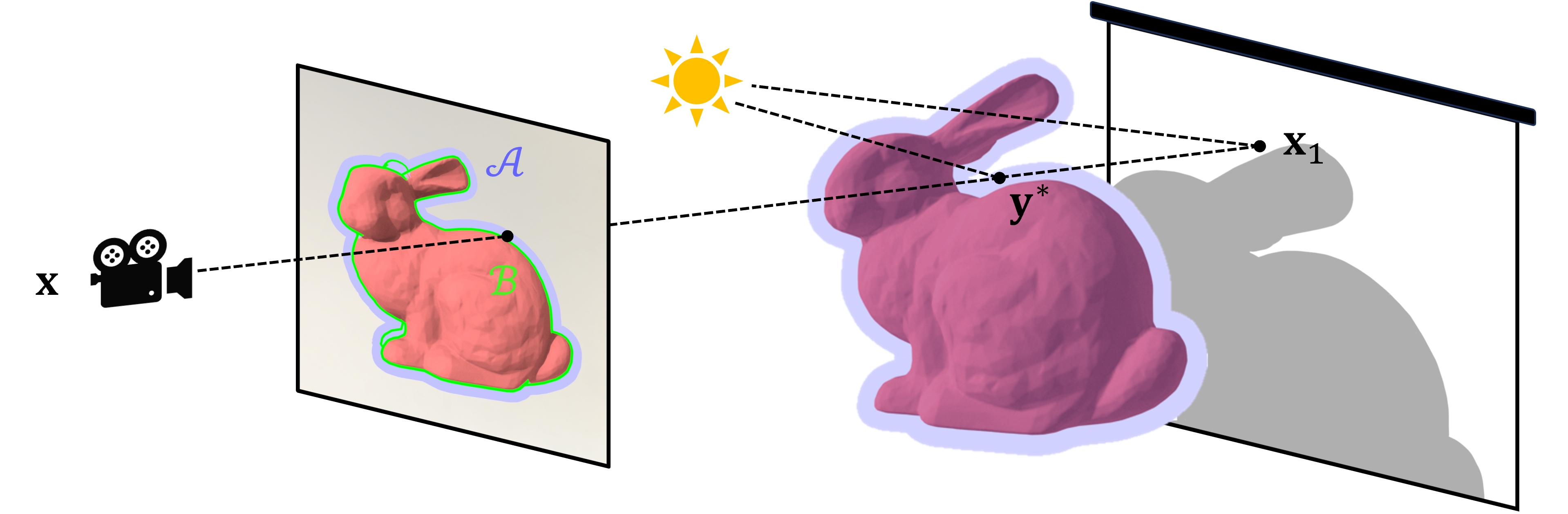
Figure 2. Method Overview. Our method relaxes the visibility boundary $\mathcal{B}$ (green) to a thin band, which we call the relaxed boundary $\mathcal{A}$ (blue). This corresponds to relaxing the surfaces to thin volumes (blue) for sampling discontinuities but retaining surface representations and physically based for forward rendering. We then take the difference between the shading at $\mathbf{y}^{*}$ and the next ray intersection point $\mathbf{x}_{1}$ to estimate the boundary integral.

3. Method

3.1. Preliminaries: Differentiating the Rendering Equation

The rendering equation states that the outgoing radiance $L_{o}$ at a point $\mathbf{x}$ in direction $\omega$ is

(1) $$L_{o}(\mathbf{x},\omega)=L_{e}(\mathbf{x},\omega)+\int_{\mathcal{S}^{2}}f_{s}(\mathbf{x},\omega^{\prime},\omega)L_{i}^{\perp}(\mathbf{x},\omega^{\prime})~{}d\sigma(\omega^{\prime}),$$

where $\omega\in\mathcal{S}^{2}$ is a vector on the unit sphere, $L_{e}$ models emission, $d\sigma$ denotes the solid angle measure, $f_{s}$ is the BSDF, and $L_{i}^{\perp}(\mathbf{x},\omega^{\prime})=L_{o}(\operatorname{\textbf{r}}(\mathbf{x},\omega^{\prime}),-\omega^{\prime})\lvert\langle\omega^{\prime},\mathbf{n}(\mathbf{x})\rangle\rvert$, where $\mathbf{r}$ is the ray intersection function. We assume that $L_{e}$ and $f_{s}$ are smooth so that discontinuities in the integrand only arise due to visibility changes at object boundaries. In the following, we abbreviate the above to

(2) $$I=\int_{\mathcal{S}^{2}}f(\omega)~{}d\sigma(\omega).$$

Our goal is to compute the derivative $\partial I/\partial\theta$ with respect to a scene parameter $\theta$ that potentially influences the placement of discontinuities. Previous work (Zhang et al., 2020; Bangaru et al., 2020) observed that this derivative can be expressed as a sum of two integrals:

(3) $$\frac{\partial I}{\partial\theta}=\int_{\mathcal{S}^{2}}\frac{\partial f(\omega)}{\partial\theta}~{}d\sigma(\omega)+\int_{\mathcal{B}}v^{\perp}(\omega)\Delta f(\omega)~{}d\tau(\omega).$$

These two terms are the interior and boundary integrals. In the latter term, $d\tau(\omega)$ denotes the arclength measure along $\mathcal{B}\subset\mathcal{S}^{2}$, the set of visibility-induced discontinuities observed at $\mathbf{x}$. Each direction $\omega\in\mathcal{B}$ on such a boundary is associated with a distant silhouette point that we label $\mathbf{x}^{*}$. The function $\Delta f(\omega)$ equals the step change in incident radiance across this oriented boundary.

The Signed Distance Function $\operatorname{SDF}:\mathbb{R}^{3}\to\mathbb{R}$ describes the distance of a point $\mathbf{x}$ to the implicit surface $\operatorname{SDF}^{-1}(0)$. This definition over the entire scene space enables us to define a normal field $\mathbf{n}(\mathbf{x})\coloneqq\nabla\operatorname{SDF}(\mathbf{x})/\|\nabla\operatorname{SDF}(\mathbf{x})\|$ that smoothly extends to positions $\mathbf{x}\in\mathbb{R}^{3}$ in the neighborhood of the surface. The normal velocity $\mathbf{v}(\mathbf{x})\coloneqq d\mathbf{x}/d\theta$ is defined as the change of the surface at $\mathbf{x}$ along its normal with respect to a perturbation of $\theta$. It equals the derivative of the following normal-aligned vector field (Stam and Schmidt, 2011):

(4) $$\mathbf{v}(\mathbf{x})=-\frac{\partial}{\partial\theta}\operatorname{SDF}(\mathbf{x})\cdot\frac{\nabla\operatorname{SDF}(\mathbf{x})}{\|\nabla\operatorname{SDF}(\mathbf{x})\|^{2}}.$$

The scalar normal velocity $\mathbf{v}^{\perp}(\mathbf{x})$ is a key quantity that measures the projection of this velocity $\mathbf{v}(\mathbf{x})$ onto the normal $\mathbf{n}$:

(5) $$\mathbf{v}^{\perp}(\mathbf{x}):=\langle\mathbf{v}(\mathbf{x}),\mathbf{n}(\mathbf{x})\rangle.$$

Each of these terms has its spherical projection. The velocity of a direction $\omega\in\mathcal{S}^{2}$ is denoted $v(\omega)\coloneqq d\omega/d\theta$. For $\omega\in\mathcal{B}$, we can further define the boundary normal $n(\omega)\in T_{\omega}\mathcal{S}^{2}$ to be the outpointing unit vector perpendicular to $\mathcal{B}$. The scalar normal velocity is then $v^{\perp}(\omega)\coloneqq\langle v(\omega),n(\omega)\rangle$. Note that we use bold notation for variables in $\mathbb{R}^{3}$ and italic for corresponding variables on $\mathcal{S}^{2}$.

To relate the spatial scalar normal velocity with its spherical projection, we observe that $\omega\in\mathcal{B}$ and its corresponding silhouette point $\mathbf{x}^{*}$ satisfies

(6) $$\mathbf{x}^{*}=\mathbf{x}+\|\mathbf{x}^{*}-\mathbf{x}\|~{}\omega.$$

Taking its derivative with respect to $\theta$ we have

(7) $$\mathbf{v}(\mathbf{x}^{*})=\frac{\partial}{\partial\theta}\|\mathbf{x}^{*}-\mathbf{x}\|\cdot\omega+\|\mathbf{x}^{*}-\mathbf{x}\|\,v(\omega).$$

Taking an inner product with respect to $n(\omega)$ on both sides yields

(8) $$\mathbf{v}^{\perp}(\mathbf{x}^{*})=\|\mathbf{x}^{*}-\mathbf{x}\|~{}v^{\perp}(\omega).$$

That is, the normal motion on the unit sphere is inversely proportional to the distance between $\mathbf{x}$ and $\mathbf{x}^{*}$ (Figure 3).

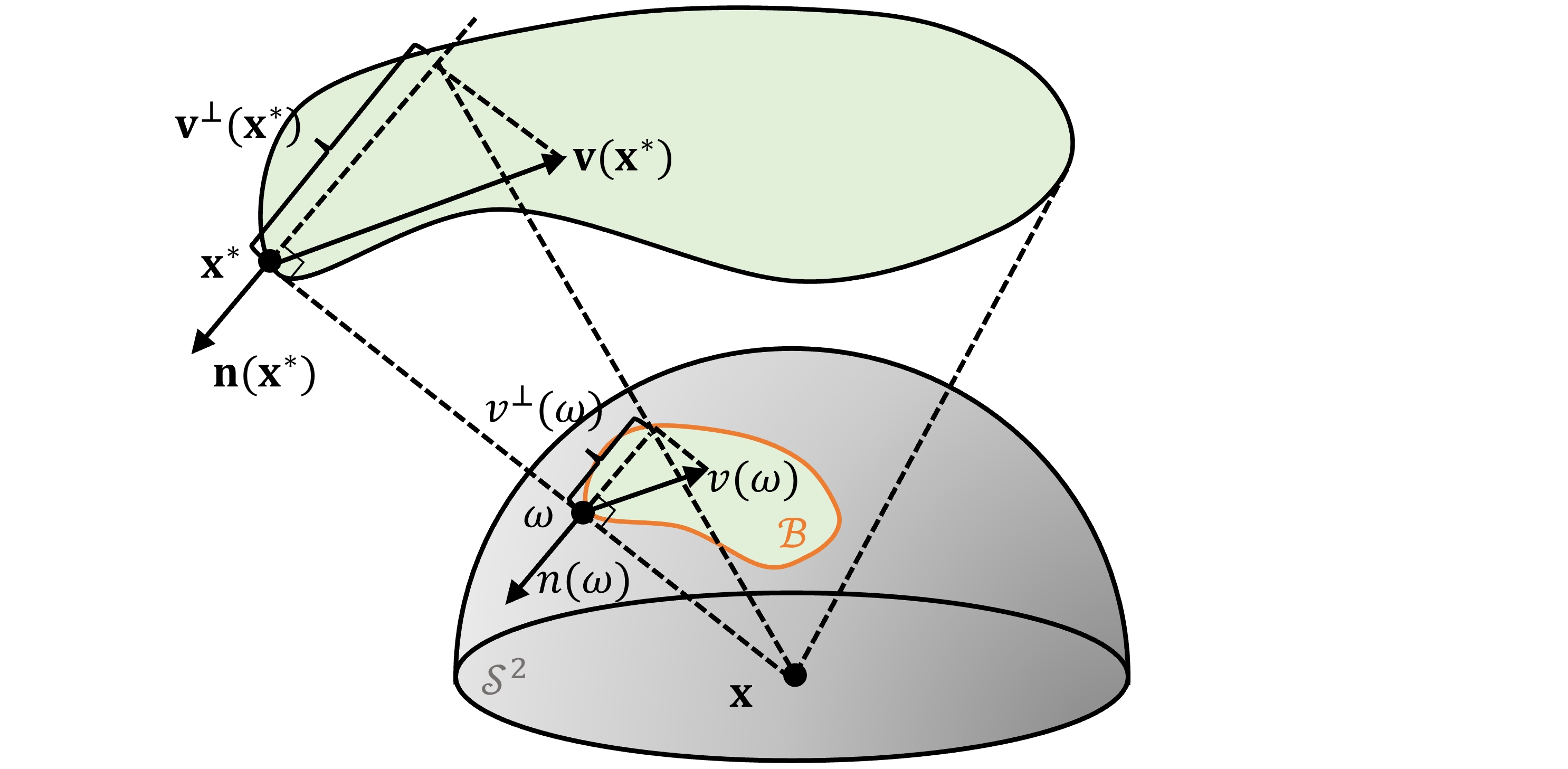
Figure 3. Normal velocity. Each direction $\omega$ in the visibility boundary $\mathcal{B}$ corresponds to a distant silhouette point $\mathbf{x}^{*}$, where the associated ray grazes an occluder. The dot products of the velocity and the normal give the normal velocities in each space, which are inversely proportional to $||\mathbf{x}-\mathbf{x}^{*}||$.

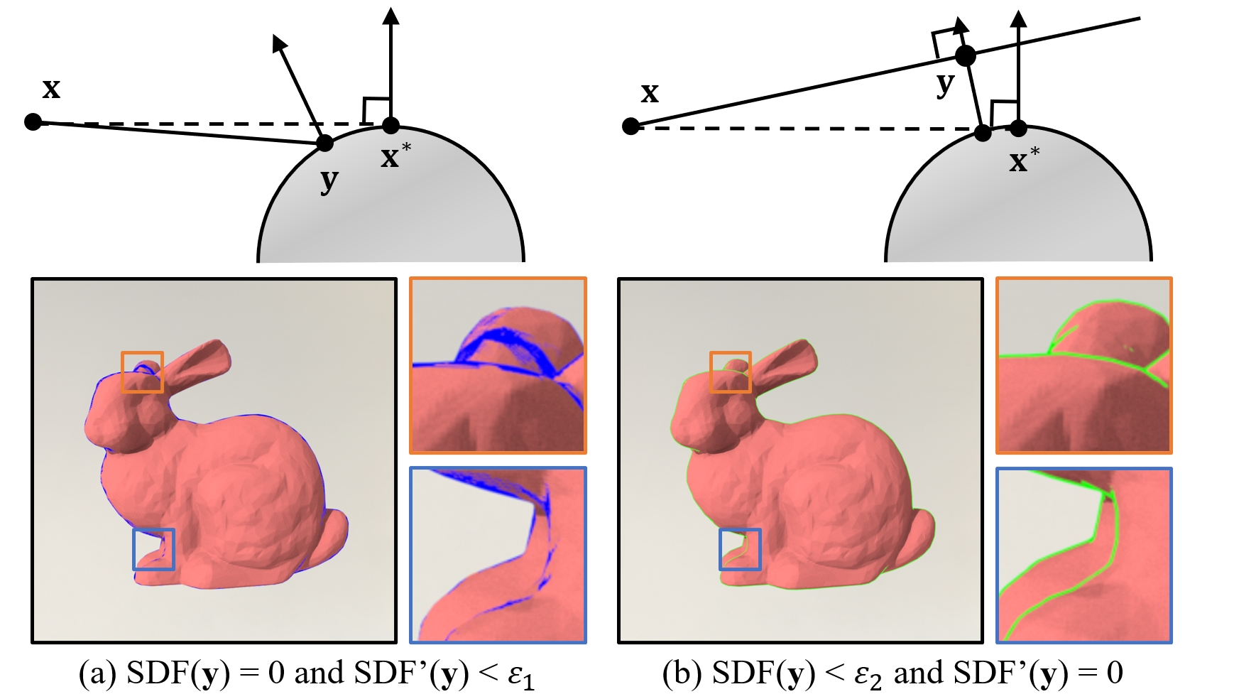
Figure 4. Relaxation. We color image plane samples whose corresponding $\mathbf{y}$s satisfy the relaxation conditions blue/green to visualize the sampling of the silhouette after relaxation. (a) Relaxing the directional derivative condition leads to rays that intersect with the surface almost tangentially. (b) Relaxing the SDF condition leads to rays that graze the surface with no intersection. Here we set $\varepsilon_{1}=0.2$ and $\varepsilon_{2}=0.002$. Even with a much smaller threshold, relaxing the SDF condition leads to uniform samples around the silhouette and will not miss parts of the silhouette.

3.2. Boundary Relaxation

Defining relaxtion

A silhouette point $\mathbf{x}^{*}$ necessarily satisfy

(9) $$\operatorname{SDF}(\mathbf{x}^{*})=0\text{ and }\operatorname{SDF^{\prime}\!}(\mathbf{x}^{*})=0$$

where $\operatorname{SDF^{\prime}\!}(\mathbf{x})$ denotes the directional derivative of $\operatorname{SDF}(\mathbf{x})$ along the ray direction at $\mathbf{x}$ (Bangaru et al., 2020; Gargallo et al., 2007). $\operatorname{SDF}(\mathbf{x}^{*})=0$ requires $\mathbf{x}^{*}$ to be on the surface, while $\operatorname{SDF^{\prime}\!}(\mathbf{x}^{*})=0$ says that $\mathbf{x}^{*}$ is a local SDF minimum along the ray. ($\mathbf{x}^{*}$ cannot be a local maximum since $\operatorname{SDF}$ is non-negative for any points on a valid path segment.) In other words, a silhouette point corresponds to a ray that tangentially intersects with a surface.

Since directly sampling the lower-dimensional silhouette is difficult, a natural idea is to relax the conditions and use nearby rays to approximate the silhouette. In Figure 4, we compare between relaxing different conditions. If we relax the $\operatorname{SDF^{\prime}\!}$ condition, we will obtain rays that almost tangentially intersect with a surface. If we relax the $\operatorname{SDF}$ condition, we will obtain rays that graze the surface with no intersection. Although relaxing $\operatorname{SDF^{\prime}\!}$ seems to give ray intersection points that resemble silhouette points, they are in practice equally hard to sample and sensitive to the curvature at the silhouette. In fact, several recent methods in this direction need to take a large relaxation (sometimes the entire surface) and then take an extra step to walk ray intersection points to the silhouette (Zhang et al., 2022a, 2023). On the other hand, if we want to use these relaxed points to directly approximate the boundary integral, it is more desirable to relax the condition on $\operatorname{SDF}$ to

(10) $$0<\operatorname{SDF}(\mathbf{y}^{*})<\varepsilon\text{ and }\operatorname{SDF^{\prime}\!}(\mathbf{y}^{*})=0$$

for some small $\varepsilon>0$. We call $\varepsilon$ the SDF threshold. We call $\mathbf{y}^{*}$ a relaxed silhouette point. We call the set of directions $\gamma$ that correspond to these relaxed silhouette points the relaxed boundary $\mathcal{A}$. Intuitively, $\mathcal{A}$ is a thin band on the unit sphere on one side of $\mathcal{B}$.

Properties of relaxation

Under this definition, there is a natural extension of the boundary integrand from the visibility boundary $\mathcal{B}$ to the relaxed boundary $\mathcal{A}$. Given some direction $\gamma\in\mathcal{A}$ and its corresponding relaxed silhouette point $\mathbf{y}^{*}$, the trick is to see $\mathbf{y}^{*}$ as a silhouette point of the $\lambda$-level set, where $\lambda=\operatorname{SDF}(\mathbf{y}^{*})$ (Figure 5). In this way, we can apply Equation 8 to talk about the scalar normal velocity of $\gamma$, and $\Delta f(\gamma)$ should be the difference of $f(\gamma)$ between missing and intersecting with the $\lambda$-level set.

Given some $\omega\in\mathcal{B}$, we also want to know the set of $\gamma\in\mathcal{A}$ that $\omega$ relaxes to. One natural thought is to extend $\omega$ along its normal direction $n(\omega)$. This would correspond to extending $\mathbf{x}^{*}$ along the normal direction $\mathbf{n}(\mathbf{x}^{*})$ until the relaxed silhouette point $\mathbf{y}^{*}$ along the ray achieves maximum relaxation $\operatorname{SDF}(\mathbf{y}^{*})=\varepsilon$. Since $n(\omega)$ is identical to $\mathbf{n}(\mathbf{x}^{*})$ and $\varepsilon$ is very small, this extension approximately gives us a segment along $\mathbf{n}(\mathbf{x}^{*})$ of length $\varepsilon$ and, scaled by the distance, a segment along $n(\omega)$ of length

(11) $$l(\omega)=\varepsilon/r$$

where $r\coloneqq\|\mathbf{x}^{*}-\mathbf{x}\|$. We call $l(\omega)$ the width of the band. This approximation by a small segment along the tangential direction is then a first-order approximation.

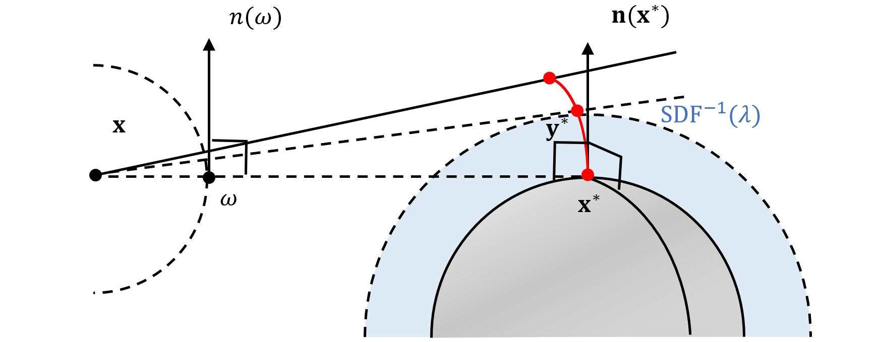
Figure 5. Relaxed silhouette point. Extending along the normal of a silhouette point $\mathbf{x}^{*}$ gives a set of relaxed silhouette points $\mathbf{y}^{*}$ (red curve) that can be approximated to first order by a line segment. A relaxed silhouette point $\mathbf{y}^{*}$ can be seen as a silhouette point of the $\lambda$-level set, where $\lambda=\operatorname{SDF}(\mathbf{y}^{*})$.

3.3. Estimating the Boundary Integral

Now that we know how to relax the lower-dimensional visibility boundary $\mathcal{B}$ to the relaxed boundary $\mathcal{A}$, it remains to ask how can we integrate over $\mathcal{A}$ to estimate the boundary integral

(12) $$I_{\mathcal{B}}=\int_{\mathcal{B}}v^{\perp}(\omega)\Delta f(\omega)~{}d\tau(\omega)$$

Given how normal extension relates silhouette points and relaxed silhouette points, a good starting point is to weigh the integrand by the width of the band

(13) $$I_{\mathcal{B}}\approx I_{\mathcal{A}}=\int_{\mathcal{A}}\frac{1}{l(\omega)}\cdot v^{\perp}(\omega)\Delta f(\omega)~{}d\sigma(\omega).$$

As discussed above, the integrand is well-defined as we can see it as the silhouette point of the $\lambda$-level set. Of course, this will only work if the integrand is continuous near the visibility boundary, which is true as long as the path segment is not tangential to multiple surfaces, which we assume is rare, and the surface BRDF is a continuous function of both position and direction. In general, it is not uncommon to regularize the appearance by spatial displacements (Fridovich-Keil and Yu et al., 2022; Rosu and Behnke, 2023).

Finally, substituting Equation 8 and 11 into Equation 13 we come to the central result of this paper, which we call the relaxed boundary integral:

(14) $$I_{\mathcal{A}} =\int_{\mathcal{A}}\frac{r}{\varepsilon}\cdot\frac{1}{r}\mathbf{v}^{\perp}(\mathbf{y}^{*})\Delta f(\omega)~{}d\sigma(\omega)$$

(15) $$=\frac{1}{\varepsilon}\int_{\mathcal{A}}\mathbf{v}^{\perp}(\mathbf{y}^{*})\Delta f(\omega)~{}d\sigma(\omega)$$

(16) $$=\frac{1}{\varepsilon}\int_{\mathcal{S}^{2}}\mathbf{v}^{\perp}(\mathbf{y}^{*})\Delta f(\omega)\mathbbm{1}_{\mathcal{A}}(\omega)~{}d\sigma(\omega).$$

A few remarks on the implications of this new integral: First, the relaxed boundary integral brings the integral domain from a lower-dimensional curve back to the entire unit sphere. This means that we can now re-use the samples for forward rendering to estimate the boundary integral, without additional projection, guiding, or data structures to help sample the silhouette. It follows that many importance sampling strategies used to estimate the forward rendering integrand $f(\omega)$ can now also benefit the estimate of $\Delta f(\omega)$. Second, the relaxed boundary integral requires minimal additional machinery. Apart from the scalar normal velocity $\mathbf{v}^{\perp}(\mathbf{y}^{*})$ and the difference term $\Delta f(\omega)$ inherited from the original boundary integral, we only need to check if a direction is inside the relaxed boundary $\mathbbm{1}_{\mathcal{A}}(\omega)$, i.e., whether there a point satisfying Equation 10 when tracing a ray along this direction. This boils down to simply solving the minimal SDF point along the ray (see Section 4).

Function Render():

      // normal path tracing

      $\omega_{1}$ = sample a direction

      $\mathbf{x}_{1}=\operatorname{\textbf{r}}(o=\mathbf{x},d=\omega_{1})$ // ray intersection

      $\omega_{2}$ = sample a second direction

      $\mathbf{x}_{2}=\operatorname{\textbf{r}}(o=\mathbf{x}_{1},d=\omega_{2})$

      $L$ = evaluate the radiance of path $(\mathbf{x},\mathbf{x}_{1},\mathbf{x}_{2})$

      // differentiable rendering

      if there exists $\mathbf{y}^{*}\in\overline{\mathbf{x}\mathbf{x}_{1}}$ then

           $\omega_{3}$ = sample a direction // resample

           $\mathbf{x}_{3}=\operatorname{\textbf{r}}(o=\mathbf{x}_{1},d=\omega_{3})$

           $L_{2}$ = evaluate the radiance of path $(\mathbf{x},\mathbf{y}^{*},\mathbf{x}_{3})$

           $\mathbf{n}(\mathbf{y}^{*}),\mathbf{v}(\mathbf{y}^{*})$ = evaluate the normal and velocity at $\mathbf{y}^{*}$

           $dL=\partial L/\partial\theta+\langle\mathbf{n}(\mathbf{y}^{*}),\mathbf{v}(\mathbf{y}^{*})\rangle(L_{2}-L)/\varepsilon$

           else if there exists $\mathbf{y}^{*}\in\overline{\mathbf{x}_{1}\mathbf{x}_{2}}$ then

                $\mathbf{n}(\mathbf{y}^{*}),\mathbf{v}(\mathbf{y}^{*})$ = evaluate the normal and velocity at $\mathbf{y}^{*}$

                $dL=\partial L/\partial\theta+\langle\mathbf{n}(\mathbf{y}^{*}),\mathbf{v}(\mathbf{y}^{*})\rangle(-L)/\varepsilon$

                else

                     $dL=\partial L/\partial\theta$ // interior only

                     end if

                    return $L$, $dL$

                    

                    

                    

ALGORITHM 1 Differentiable Renderer

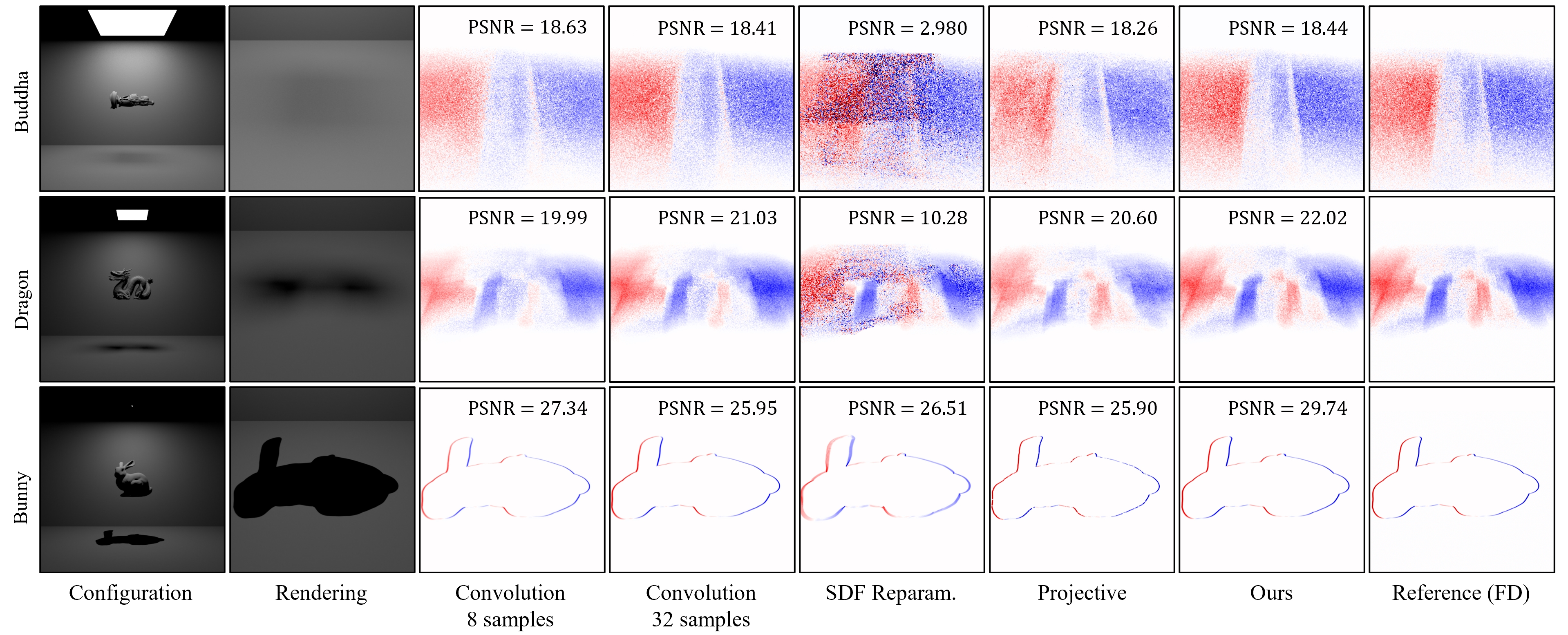
Figure 6. Forward derivative. We use forward-mode differentiation to compute the derivative of the rendered image with respect to a translation in the $x$ axis. We test different shapes under different sizes of square area light and compare with SDF convolution (Bangaru et al., 2020), SDF Reparameterization (Vicini et al., 2022), and mesh Projective Sampling (Zhang et al., 2023). For all tests we use a direct integrator with $512\times 512$ resolution and $1024$ spp.

4. Implementation

Solving relaxed silhouette point

While sampling the silhouette is difficult, sampling relaxed silhouette points is much easier. During sphere tracing, we can compute the directional derivative of the intermediate steps and, together with the SDF value, check if they are close to being a relaxed silhouette point. Specifically, if in the previous step the directional derivative is negative and at this step the derivative becomes positive, then this would be a signal that we are near a local minimum. Among all such intermediate steps, we choose the one with the smallest SDF value as our initial guess and run the bisection method for $12$ iterations to pinpoint the relaxed silhouette point.

Estimating relaxed boundary integral

In algorithm 1, we give the pseudo code for the direct integrator that we use for all our experiments. In addition to normal path tracing, if there exists a relaxed silhouette point $\mathbf{y}^{*}$ during the primary sphere tracing process, we need to re-evaluate the shading at $\mathbf{y}^{*}$. Taking its difference with the shading at $\mathbf{x}_{1}$ gives us the delta difference term. For secondary rays, note one side of the visibility boundary is always occluded, so we no longer need to evaluate the shading at the relaxed silhouette point. We estimate the interior integral in Equation 3 using automatic differentiation except for the ray intersection process, whose derivatives are computed analytically after the sphere tracing process in the same way as in (Vicini et al., 2022; Bangaru et al., 2022).

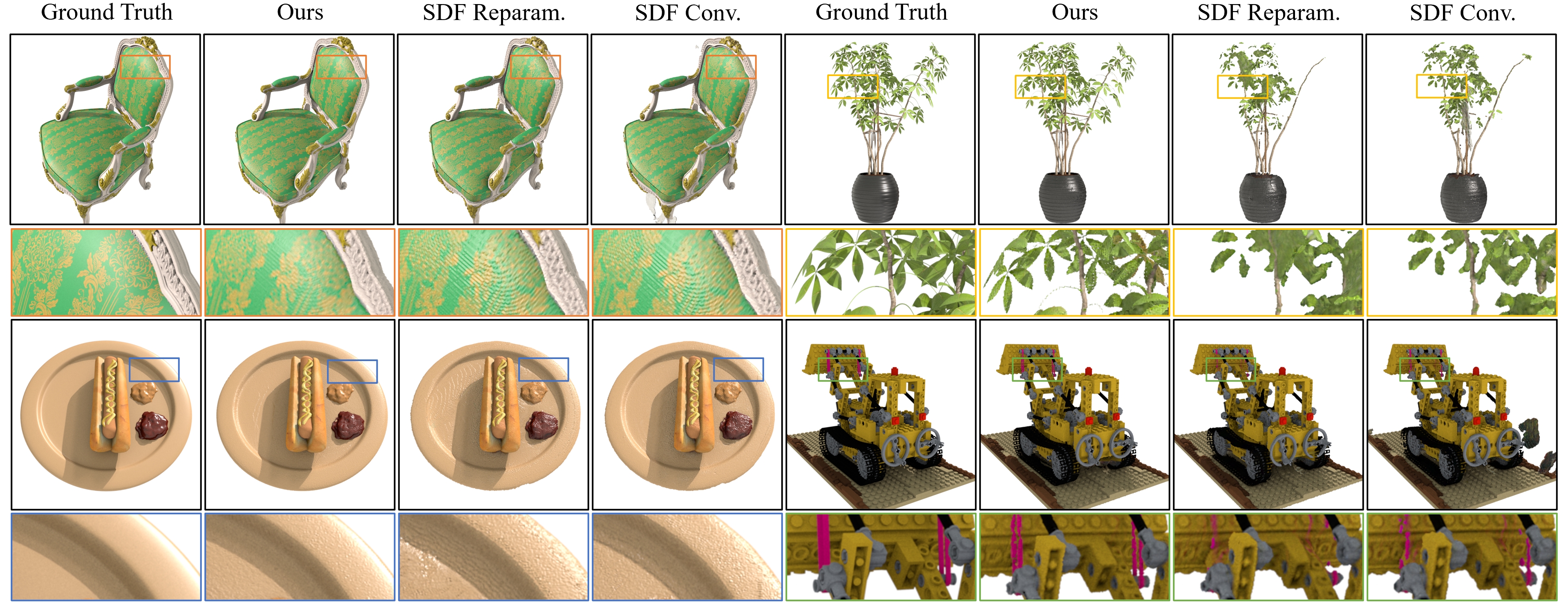
Figure 7. Side-by-side comparison. We compare the final inverse rendering of SDF Convolution (8 auxiliary spp), SDF Reparameterization, and our method using the same optimization setup: in total we run $5000$ iterations optimizing $50$ views; in each iteration, we optimize a batch of $5$ views, rendered with $512\times 512$ resolution and $64$ spp. In all test cases, our method results in comparable or more accurate reconstructions.

	Novel Views			Relighting (High)			Relighting (Low)			Chamfer L1	Time
	PSNR$\uparrow$	SSIM$\uparrow$	LPIPS$\downarrow$	PSNR$\uparrow$	SSIM$\uparrow$	LPIPS$\downarrow$	PSNR$\uparrow$	SSIM$\uparrow$	LPIPS$\downarrow$	Distance$\downarrow$	per step
SDF Conv.	29.583	0.9361	0.0856	21.119	0.9205	0.0917	26.759	0.9140	0.099	0.0080	10.85s
SDF Reparam.	33.141	0.9509	0.0586	26.092	0.9379	0.0616	29.039	0.9290	0.0744	0.0073	7.08s
SDF Reparam. (hqq)	29.621	0.9302	0.0943	22.262	0.9138	0.0996	30.385	0.9317	0.0723	0.0122	5.00s
Ours (trilinear)	37.550	0.9812	0.0216	31.340	0.9722	0.0194	31.618	0.9574	0.0372	0.0052	2.23s
Ours (cubic)	37.466	0.9800	0.0234	31.744	0.9729	0.0200	32.189	0.9582	0.0375	0.0047	4.03s

Table 1. Quantative measurements. We measure quantitatively the performance of different methods on synthetic Chair, Lego, Hotdog, Ficus, and Drum. For 2D measurements, we test novel view rendering and relighting on a high-contrast and a low-contrast environment map. For 3D measurements, we test the Chamfer L1 distance using random sample points on the ground truth mesh. We use the same optimization setup as in Figure 7 and additionally run SDF Reparameterization using their released hqq setup. Since previous methods require cubic interpolation of the SDF grid, we further test our method on both trilinear and cubic interpolation for better reference.

5. results

We implemented our differentiable direct integrator using the Mitsuba3 (Jakob et al., 2022) Python package. Our implementation runs on CUDA and LLVM backends, and the results in this section were obtained using the CUDA backend on an NVIDIA RTX 3090.

5.1. Validation

Forward derivatives

We validate our method by computing the forward derivative of the rendered image with respect to a single translation parameter. Since our method focuses on estimating the boundary integral, we place an object under a top area light and above a bottom plane and set the camera to look at the cast shadow of the object onto the bottom plane. In this way, all gradients come from the boundary integral. For reference, we use finite difference (FD) with a step size of $10^{-4}$. We also compare our results with SDF Convolution (Bangaru et al., 2020), SDF reparameterization, and mesh projective sampling (Zhang et al., 2023). In Figure 6, we can see that our method results in the highest PSNR under different sizes of area lights.

Inverse rendering

We further test our differentiable renderer on end-to-end inverse rendering tasks. Note our focus is on showing the effectiveness of our differentiable renderer on downstream applications. We intentionally use a conservative setup and do not push for state-of-the-art performance.

In all our reconstructions, we use environment maps for lighting and perspective cameras distributed on the unit hemisphere. We restrict the SDF to be within the unit cube and use either diffuse or principled BSDF as our material. We use voxel grids to represent the SDF, albedo, roughness, and metallic components of the scene. For optimization, we initialize with a sphere and run an Adam optimizer (Kingma and Ba, 2015) with a learning rate of $10^{-2}$. We adopt a coarse-to-fine optimization scheme that upscales the grid resolution by $2$ each time. We predetermined the upscale iterations by giving enough iterations during each resolution. Within each iteration, we compute the L1 loss between a batch of reference images and rendered images. To regularize the SDF to satisfy the eikonal constraint, we redistance the SDF after every iteration using the same fast sweeping method implementation of Vicini et. al. (Vicini et al., 2022).

In Figure 10, we demonstrate the optimization process on a variety of shapes. The high-genus Voronoi Bunny showcases that we can handle complex geometry with frequent boundaries. Subsequently, we jointly optimize the geometry and the material of Lego, Chair, Hotdog, Ficus, and Drum for more complete inverse rendering. We take the original Blender models of the NeRF Synthetic dataset (Mildenhall et al., 2020) and adapt them to modified Mitsuba versions. Finally, to emphasize the physically-based nature of our differentiable renderer, we reconstruct the Logo by only looking at its cast shadow on four planes. We intentionally design the lighting condition so that the shadows largely overlap with each other, adding difficulty to the reconstruction.

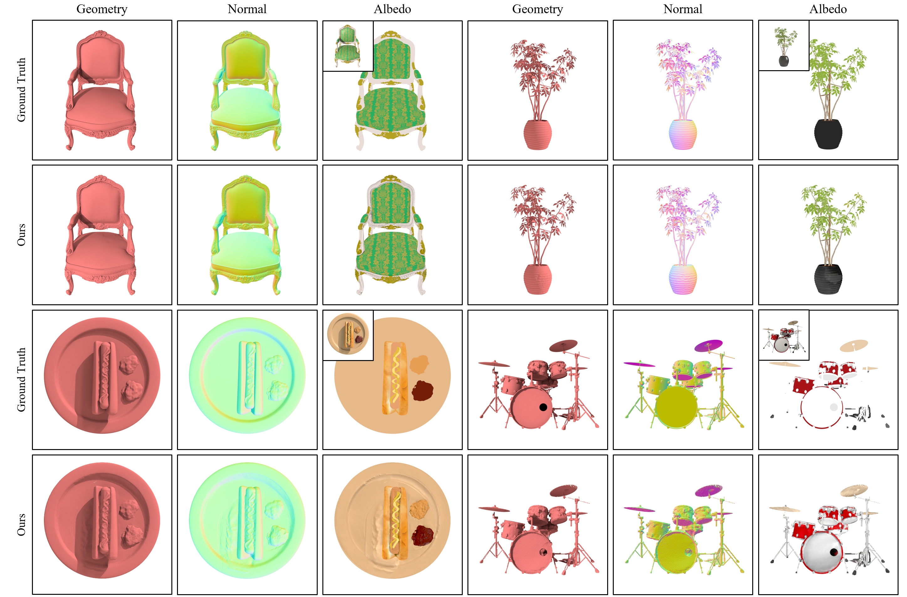
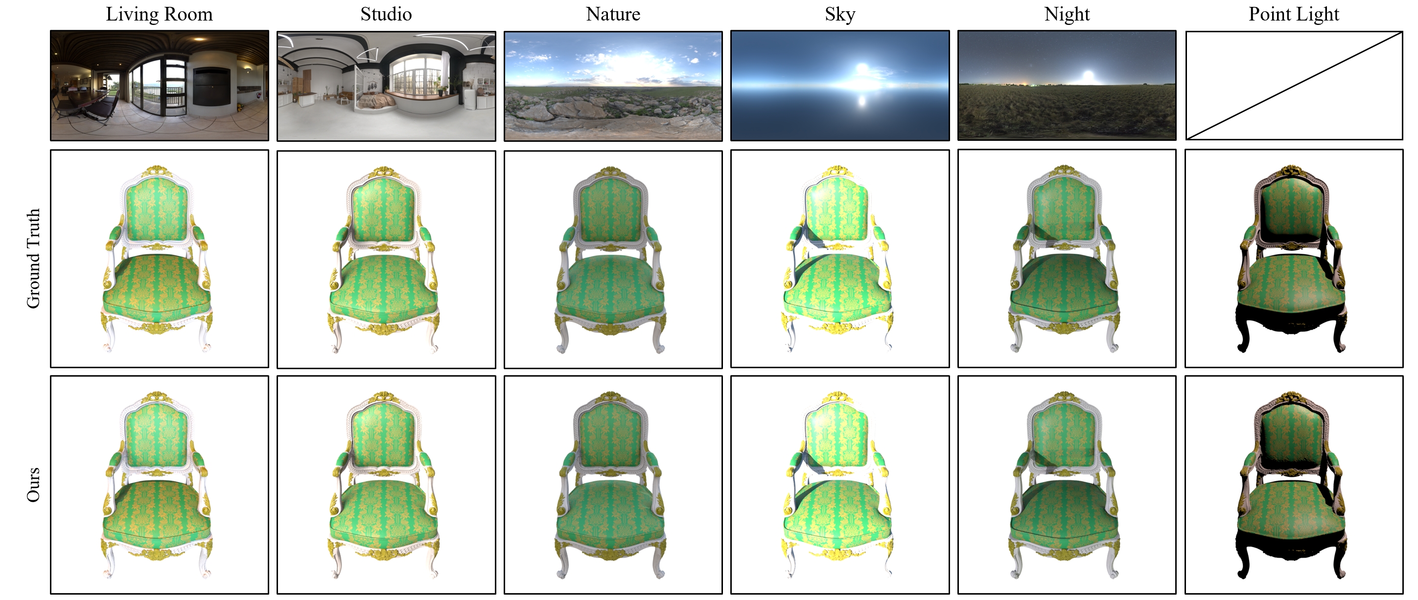
Figure 11. Inverse rendering and relighting. The physically-based nature of our differentiable renderer enables joint optimization of geometry/material and hence easy relighting. Here we visualize the geometry, normal, and albedo of our final inverse rendering and the relighting under various lighting conditions. Note how we can largely disentangle shading effects from the albedo (in comparison with the top right rendering).

When it comes to inverse rendering, physically based differentiable renderers can easily support a wide range of materials and the disentanglement of geometry and material. In Figure 11, we visualize the geometry, normal, and albedo of our final inverse rendering results, as well as the relighting of the Chair under various lighting conditions. In general, we can correctly separate the geometry and material from the complex shading effects, such as the case shadow on the Chiar and the dense self-occlusions of the Ficus.

In Figure 7, we show a side-by-side comparison between SDF Convolution, SDF Reparameterization, and our method. In Table 1, we quantitatively measure the performance of different methods. For all tests on all shapes, we achieve comparable or superior results than previous methods. We think that sufficient sampling of the silhouette enables us to reconstruct fine structures, such as the stem of the Ficus and the belt on the Lego. This also helps reduce the gradient variance to achieve smoother surfaces on the Chair and Hotdog. Gradient variance is also important for improving robustness: extreme gradients could lead to too large optimization steps and hence irremediable divergence, as seen in the Chair and Lego reconstruction using SDF Convolution.

5.2. Abalation Study

The SDF threshold $\varepsilon$ is an important hyperparameter that controls how much we relax the visibility boundary. As $\varepsilon$ increases, we smooth out the boundary more and the bias increases. However, it is also not desirable to keep decreasing $\varepsilon$. A higher $\varepsilon$ enhances the possibility of sampling relaxed silhouette points, so the gradients have less variance (Figure 8). We refer to this phenomenon as the bias-variance tradeoff of $\varepsilon$. In all our reconstructions, where the target object is within a unit cube, we set $\varepsilon=10^{-4}$ to achieve the best of both worlds.

In addition to setting an optimal $\varepsilon$ for optimizations inside the unit cube, we would also want to know the feasible range of $\varepsilon$. This would be particularly important if we want our differentiable renderer to work on large scenes, where the distances of different objects to the camera can differ drastically. In Figure 9, we use the same shadow optimization setup of Logo as in Figure 10, which helps roll out the influence of the interior integral. It turns out that our differentiable renderer works quite robustly with different scales of $\varepsilon$. In all cases, our differentiable render succeeded in reconstructing the overall geometry. When $\varepsilon=10^{-2}$, too much blurring of the silhouette causes tiny floaters. When $\varepsilon=10^{-6}$, insufficient sampling of the silhouette causes the optimization to not fully converge.

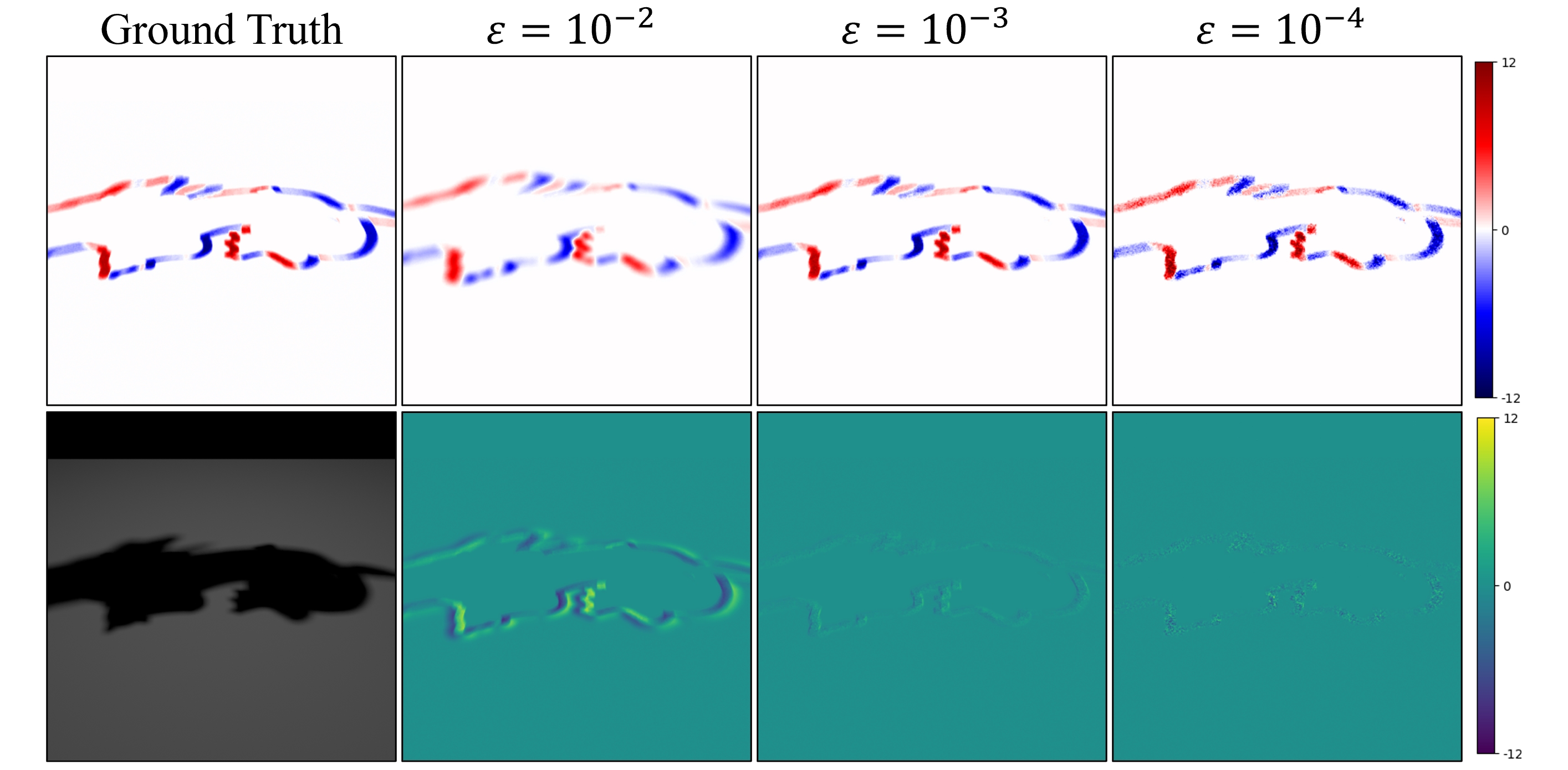
Figure 8. Bias-variance tradeoff. We show the effect of the SDF threshold on the gradients. This first row shows the reference and our forward derivatives, and the second row shows the rendered image and the difference between our forward derivatives and the reference. As $\varepsilon$ gets lower, the gradients become noisier, but at the same time only Monte Carlo noise is observed in the difference. Here we compute our forward derivatives using $256$ spp.

5.3. Limitations

Bias

The approximation of the silhouette through relaxed silhouette points is essentially biased. However, embracing nonzero bias, in turn, enables us to achieve architectural simplicity and efficient discontinuity sampling. We show through a series of experiments that the bias is well-controlled and would not interfere with the downstream applications of our differentiable renderer.

Tuning SDF threshold

The optimal choice of the SDF threshold $\varepsilon$ might depend on concretely how far the objects are to the camera, which then might require tuning of $\varepsilon$. For this reason, we show that our method is not sensitive to $\varepsilon$ and supports a wide range of feasible $\varepsilon$. Users of our differentiable renderer should only need to tune the order of $\varepsilon$.

Solving relaxed silhouette point

Our relaxation scheme specifically asks for points within a certain distance to the surface. This means that we need to support the query of the distance of an arbitrary point to the surface, and hence we choose SDF as our surface representation. At the same time, this also means that our relaxed boundary integral can be extended to other representations, as long as there exists an efficient way to satisfy this query.

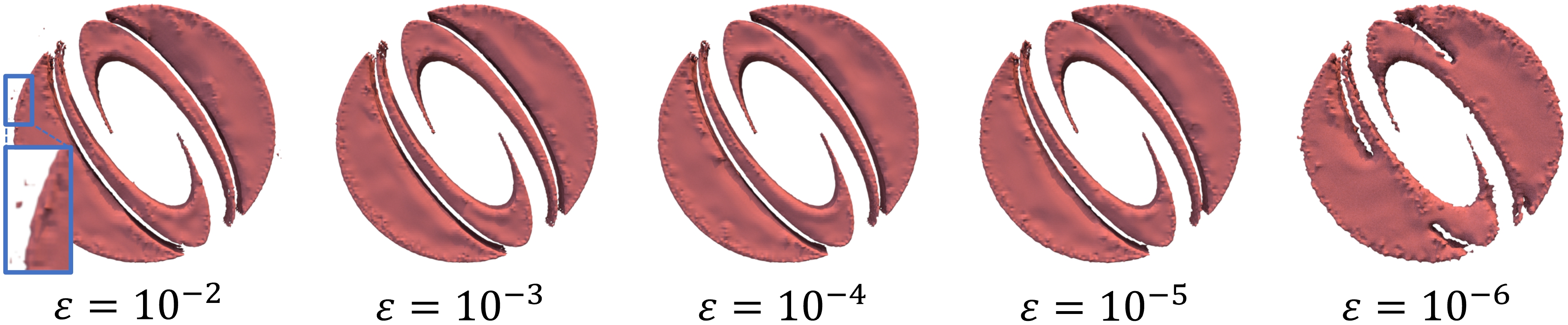
Figure 9. Effect of $\varepsilon$. Our differentiable renderer works on a wide range of $\varepsilon$. However, too large $\varepsilon$ blurs the silhouette too much and causes floaters, while too little $\varepsilon$ leads to insufficient sampling of the silhouette and causes slower convergence.

6. Conclusion

We present a novel differentiable rendering method of SDFs that is simple, robust, accurate, and efficient. Our relaxed boundary integral provides a new perspective to solving the long-standing silhouette sampling problem: through proper relaxation of the silhouette, we are able to use nearby Monte Carlo samples to directly approximate it. We test our differentiable renderer in downstream inverse rendering applications and achieve comparable or superior performance to previous methods.

For future work, one direction is to extend the relaxed boundary integral to support other shape representations. In addition, the constant $1/\varepsilon$ factor in the relaxed boundary integral can be seen as a uniform weighting of all relaxed silhouette points. Investigating better weighting schemes to reduce bias would be another interesting open question.

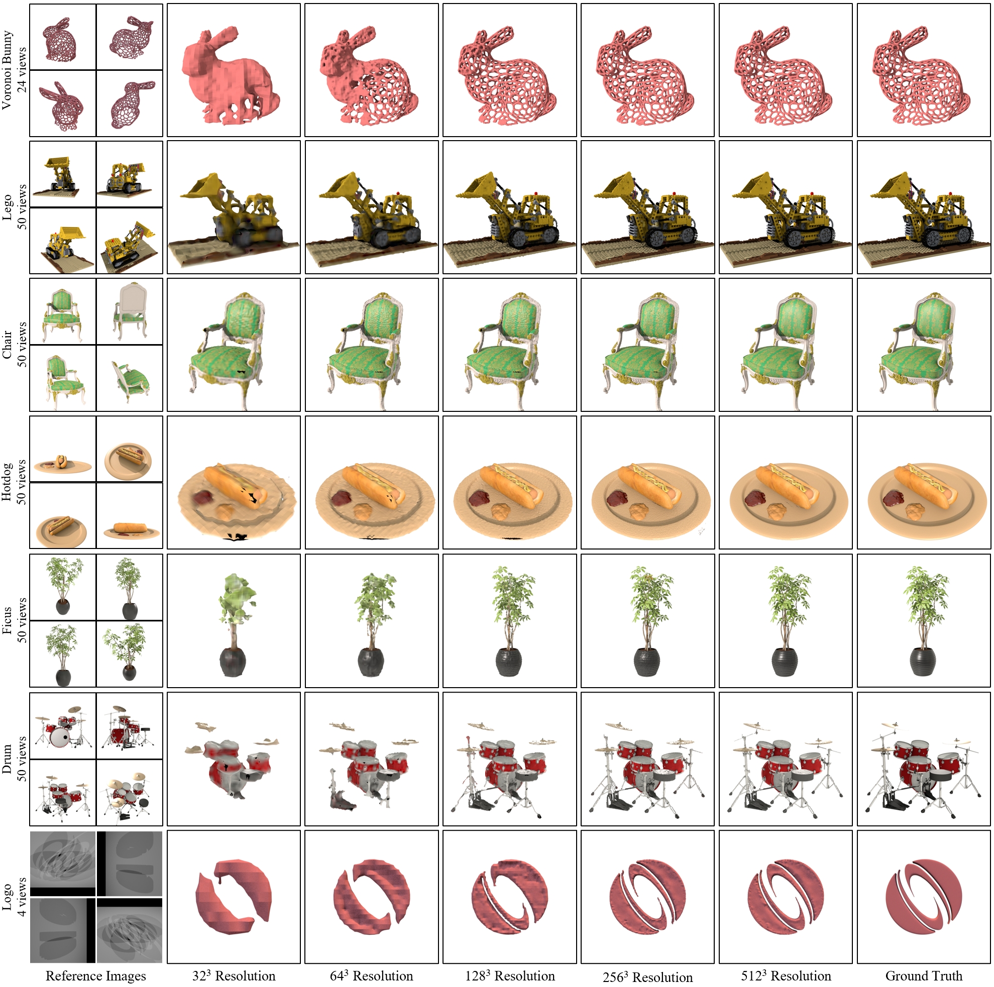
Figure 10. Optimization Process. We demonstrate the optimization process on a variety of shapes. For Voronoi Bunny, we only optimize the geometry. For Lego, we assume known diffuse material and jointly optimize the SDF and the albedo. For Chair, Hotdog, and Ficus, we optimize the SDF and a principled material (albedo and roughness). For Drum, we also add a metallic component. For Logo, we optimize the geometry by looking only at its cast shadow onto fixed walls. Voronoi Bunny from (Mehta et al., 2022). Lego $\copyright$Heinzelnisse. Drum $\copyright$bryanajones. Logo from (Vicini et al., 2022).

References

- (1)
- Bangaru et al. (2022) Sai Bangaru, Michael Gharbi, Tzu-Mao Li, Fujun Luan, Kalyan Sunkavalli, Milos Hasan, Sai Bi, Zexiang Xu, Gilbert Bernstein, and Fredo Durand. 2022. Differentiable Rendering of Neural SDFs through Reparameterization. In ACM SIGGRAPH Asia 2022 Conference Proceedings (Daegu, Republic of Korea) (SIGGRAPH Asia ’22). Association for Computing Machinery, New York, NY, USA, Article 22, 9 pages. https://doi.org/10.1145/3550469.3555397
- Bangaru et al. (2020) Sai Bangaru, Tzu-Mao Li, and Frédo Durand. 2020. Unbiased Warped-Area Sampling for Differentiable Rendering. ACM Trans. Graph. 39, 6 (2020), 245:1–245:18.
- Cole et al. (2021) Forrester Cole, Kyle Genova, Avneesh Sud, Daniel Vlasic, and Zhoutong Zhang. 2021. Differentiable surface rendering via non-differentiable sampling. In Proceedings of the IEEE/CVF International Conference on Computer Vision. 6088–6097.
- Fridovich-Keil and Yu et al. (2022) Fridovich-Keil and Yu, Matthew Tancik, Qinhong Chen, Benjamin Recht, and Angjoo Kanazawa. 2022. Plenoxels: Radiance Fields without Neural Networks. In CVPR.
- Gargallo et al. (2007) Pau Gargallo, Emmanuel Prados, and Peter Sturm. 2007. Minimizing the Reprojection Error in Surface Reconstruction from Images. In 2007 IEEE 11th International Conference on Computer Vision. 1–8. https://doi.org/10.1109/ICCV.2007.4409003
- Hazineh et al. (2022) Dean S. Hazineh, Soon Wei Daniel Lim, Zhujun Shi, Federico Capasso, Todd Zickler, and Qi Guo. 2022. D-Flat: A Differentiable Flat-Optics Framework for End-to-End Metasurface Visual Sensor Design. arXiv:2207.14780 [physics.optics]
- Jakob et al. (2022) Wenzel Jakob, Sébastien Speierer, Nicolas Roussel, Merlin Nimier-David, Delio Vicini, Tizian Zeltner, Baptiste Nicolet, Miguel Crespo, Vincent Leroy, and Ziyi Zhang. 2022. Mitsuba 3 renderer. https://mitsuba-renderer.org.
- Kang et al. (2022) Wu Kang, Fu Xiao-Ming, Renjie Chen, and Ligang Liu. 2022. Survey on computational 3D visual optical art design. Visual computing for industry, biomedicine, and art 5 (12 2022), 31. https://doi.org/10.1186/s42492-022-00126-z
- Kerbl et al. (2023) Bernhard Kerbl, Georgios Kopanas, Thomas Leimkühler, and George Drettakis. 2023. 3D Gaussian Splatting for Real-Time Radiance Field Rendering. ACM Transactions on Graphics 42, 4 (July 2023). https://repo-sam.inria.fr/fungraph/3d-gaussian-splatting/
- Kingma and Ba (2015) Diederik Kingma and Jimmy Ba. 2015. Adam: A Method for Stochastic Optimization. In International Conference on Learning Representations (ICLR). San Diega, CA, USA.
- Laine et al. (2020) Samuli Laine, Janne Hellsten, Tero Karras, Yeongho Seol, Jaakko Lehtinen, and Timo Aila. 2020. Modular Primitives for High-Performance Differentiable Rendering. ACM Transactions on Graphics 39, 6 (2020).
- Li et al. (2018) Tzu-Mao Li, Miika Aittala, Frédo Durand, and Jaakko Lehtinen. 2018. Differentiable Monte Carlo Ray Tracing through Edge Sampling. ACM Trans. Graph. (Proc. SIGGRAPH Asia) 37, 6 (2018), 222:1–222:11.
- Li et al. (2023) Zhaoshuo Li, Thomas Müller, Alex Evans, Russell H Taylor, Mathias Unberath, Ming-Yu Liu, and Chen-Hsuan Lin. 2023. Neuralangelo: High-Fidelity Neural Surface Reconstruction. In IEEE Conference on Computer Vision and Pattern Recognition (CVPR).
- Lin et al. (2023) Chen-Hsuan Lin, Jun Gao, Luming Tang, Towaki Takikawa, Xiaohui Zeng, Xun Huang, Karsten Kreis, Sanja Fidler, Ming-Yu Liu, and Tsung-Yi Lin. 2023. Magic3D: High-Resolution Text-to-3D Content Creation. In IEEE Conference on Computer Vision and Pattern Recognition (CVPR).
- Liu et al. (2019) Shichen Liu, Tianye Li, Weikai Chen, and Hao Li. 2019. Soft Rasterizer: A Differentiable Renderer for Image-based 3D Reasoning. The IEEE International Conference on Computer Vision (ICCV) (Oct 2019).
- Liu et al. (2020) Shaohui Liu, Yinda Zhang, Songyou Peng, Boxin Shi, Marc Pollefeys, and Zhaopeng Cui. 2020. Dist: Rendering deep implicit signed distance function with differentiable sphere tracing. In Proceedings of the IEEE/CVF Conference on Computer Vision and Pattern Recognition. 2019–2028.
- Loper and Black (2014) Matthew M Loper and Michael J Black. 2014. OpenDR: An approximate differentiable renderer. In Computer Vision–ECCV 2014: 13th European Conference, Zurich, Switzerland, September 6-12, 2014, Proceedings, Part VII 13. Springer, 154–169.
- Loubet et al. (2019) Guillaume Loubet, Nicolas Holzschuch, and Wenzel Jakob. 2019. Reparameterizing Discontinuous Integrands for Differentiable Rendering. Transactions on Graphics (Proceedings of SIGGRAPH Asia) 38, 6 (Dec. 2019). https://doi.org/10.1145/3355089.3356510
- Mehta et al. (2022) Ishit Mehta, Manmohan Chandraker, and Ravi Ramamoorthi. 2022. A Level Set Theory for Neural Implicit Evolution under Explicit Flows. arXiv preprint arXiv:2204.07159 (2022).
- Mildenhall et al. (2020) Ben Mildenhall, Pratul P. Srinivasan, Matthew Tancik, Jonathan T. Barron, Ravi Ramamoorthi, and Ren Ng. 2020. NeRF: Representing Scenes as Neural Radiance Fields for View Synthesis. In ECCV.
- Rakotosaona et al. (2023) Marie-Julie Rakotosaona, Fabian Manhardt, Diego Martin Arroyo, Michael Niemeyer, Abhijit Kundu, and Federico Tombari. 2023. NeRFMeshing: Distilling Neural Radiance Fields into Geometrically-Accurate 3D Meshes. In International Conference on 3D Vision (3DV).
- Rosu and Behnke (2023) Radu Alexandru Rosu and Sven Behnke. 2023. PermutoSDF: Fast Multi-View Reconstruction with Implicit Surfaces using Permutohedral Lattices. In IEEE/CVF Conference on Computer Vision and Pattern Recognition (CVPR).
- Stam and Schmidt (2011) Jos Stam and Ryan Schmidt. 2011. On the velocity of an implicit surface. ACM Trans. Graph. 30, 3, Article 21 (may 2011), 7 pages. https://doi.org/10.1145/1966394.1966400
- Sun et al. (2023) Cheng Sun, Guangyan Cai, Zhengqin Li, Kai Yan, Cheng Zhang, Carl Marshall, Jia-Bin Huang, Shuang Zhao, and Zhao Dong. 2023. Neural-PBIR Reconstruction of Shape, Material, and Illumination. arxiv (2023).
- Tang et al. (2022) Jiaxiang Tang, Hang Zhou, Xiaokang Chen, Tianshu Hu, Errui Ding, Jingdong Wang, and Gang Zeng. 2022. Delicate Textured Mesh Recovery from NeRF via Adaptive Surface Refinement. arXiv preprint arXiv:2303.02091 (2022).
- Verbin et al. (2023) Dor Verbin, Ben Mildenhall, Peter Hedman, Jonathan T. Barron, Todd Zickler, and Pratul P. Srinivasan. 2023. Eclipse: Disambiguating Illumination and Materials using Unintended Shadows. arXiv (2023).
- Vicini et al. (2022) Delio Vicini, Sébastien Speierer, and Wenzel Jakob. 2022. Differentiable Signed Distance Function Rendering. Transactions on Graphics (Proceedings of SIGGRAPH) 41, 4 (July 2022), 125:1–125:18. https://doi.org/10.1145/3528223.3530139
- Wang et al. (2021) Peng Wang, Lingjie Liu, Yuan Liu, Christian Theobalt, Taku Komura, and Wenping Wang. 2021. NeuS: Learning Neural Implicit Surfaces by Volume Rendering for Multi-view Reconstruction. NeurIPS (2021).
- Yariv et al. (2021) Lior Yariv, Jiatao Gu, Yoni Kasten, and Yaron Lipman. 2021. Volume rendering of neural implicit surfaces. In Thirty-Fifth Conference on Neural Information Processing Systems.
- Yariv et al. (2023) Lior Yariv, Peter Hedman, Christian Reiser, Dor Verbin, Pratul P. Srinivasan, Richard Szeliski, Jonathan T. Barron, and Ben Mildenhall. 2023. BakedSDF: Meshing Neural SDFs for Real-Time View Synthesis. arXiv (2023).
- Yariv et al. (2020) Lior Yariv, Yoni Kasten, Dror Moran, Meirav Galun, Matan Atzmon, Basri Ronen, and Yaron Lipman. 2020. Multiview Neural Surface Reconstruction by Disentangling Geometry and Appearance. Advances in Neural Information Processing Systems 33 (2020).
- Zhang et al. (2020) Cheng Zhang, Bailey Miller, Kai Yan, Ioannis Gkioulekas, and Shuang Zhao. 2020. Path-Space Differentiable Rendering. ACM Trans. Graph. 39, 4 (2020), 143:1–143:19.
- Zhang et al. (2022a) Kai Zhang, Fujun Luan, Zhengqi Li, and Noah Snavely. 2022a. IRON: Inverse Rendering by Optimizing Neural SDFs and Materials from Photometric Images. In IEEE Conf. Comput. Vis. Pattern Recog.
- Zhang et al. (2021) Kai Zhang, Fujun Luan, Qianqian Wang, Kavita Bala, and Noah Snavely. 2021. PhySG: Inverse Rendering with Spherical Gaussians for Physics-based Material Editing and Relighting. In The IEEE/CVF Conference on Computer Vision and Pattern Recognition (CVPR).
- Zhang et al. (2022b) Yuanqing Zhang, Jiaming Sun, Xingyi He, Huan Fu, Rongfei Jia, and Xiaowei Zhou. 2022b. Modeling Indirect Illumination for Inverse Rendering. In CVPR.
- Zhang et al. (2023) Ziyi Zhang, Nicolas Roussel, and Wenzel Jakob. 2023. Projective Sampling for Differentiable Rendering of Geometry. Transactions on Graphics (Proceedings of SIGGRAPH Asia) 42, 6 (Dec. 2023). https://doi.org/10.1145/3618385