A Generalized Difference-in-Differences Estimator for Unbiased Estimation of Desired Estimands from Staggered Adoption and Stepped-Wedge Settings
Abstract
Staggered treatment adoption arises in the evaluation of policy impact and implementation in a variety of settings. This occurs in both randomized stepped-wedge trials and non-randomized quasi-experimental designs using causal inference methods based on difference-in-differences analysis. In both settings, it is crucial to carefully consider the target estimand and possible treatment effect heterogeneities in order to estimate the effect without bias and in an interpretable fashion. This paper proposes a novel non-parametric approach to this estimation for either setting. By constructing an estimator using two-by-two difference-in-difference comparisons as building blocks with arbitrary weights, the investigator can select weights to target the desired estimand in an unbiased manner under assumed treatment effect homogeneity, and minimize the variance under an assumed working covariance structure. This provides desirable bias properties with a relatively small sacrifice in variance and power by using the comparisons efficiently. The method is demonstrated on toy examples to show the process, as well as in the re-analysis of a stepped wedge trial on the impact of novel tuberculosis diagnostic tools. A full algorithm with R code is provided to implement this method. The proposed method allows for high flexibility and clear targeting of desired effects, providing one solution to the bias-variance-generalizability tradeoff.
Keywords: Bias-variance tradeoff, causal inference, cluster-randomized trials, non-parametric estimation, permutation inference, quasi-experiments
1 Introduction
Staggered treatment adoption occurs in a wide variety of settings, including both observational and randomized contexts. In observational and quasi-experimental studies, panel data methods are commonly used to analyze the effect of a policy implementation or an exogenous shock. Stepped-wedge cluster-randomized trials have also become a common approach for the analysis of health, education, or other social policies, especially with a phased or gradual implementation. Across settings, the analysis of the data generated from staggered treatment settings requires careful consideration of the desired estimand, assumptions about the treatment effect, consideration of heterogeneity across units, time periods, and treatment regimens, and appropriate consideration of variance and correlation.
This complexity has led to the development of a wide array of methods, commonly found in the econometrics literature surrounding panel data, difference-in-differences (DID), and staggered treatment adoption and in the biostatistics literature surrounding stepped-wedge trials (SWTs). Key developments in SWTs include approaches to interpret the targeted estimand (see, e.g., Twisk et al. (2016)), design-based considerations (see, e.g., Matthews & Forbes (2017) and Li et al. (2023)), robust inference (see, e.g., Wang & De Gruttola (2017), Hughes et al. (2020), Maleyeff et al. (2023)), and a variety of analytic approaches, discussed below. While development in both areas is still very much ongoing, recent reviews of the staggered adoption literature can be found in, among others, Baker et al. (2022), de Chaisemartin & D’Haultfœuille (2023), Roth et al. (2023), and Borusyak et al. (2024).
What these new developments generally share is an acknowledgment of the need for careful selection of the target estimand and modeling of the treatment effect in order to estimate that estimand without bias. In the stepped-wedge setting, this is often done using a parametric or semi-parametric model for the treatment effect that can account for heterogeneity as in Hooper et al. (2016), Nickless et al. (2018), Kenny et al. (2022), Maleyeff et al. (2023), and Lee & Cheung (2024). It can, however, also be done using appropriate weighting of non-parametric estimators like those proposed by Thompson et al. (2018) and Kennedy‐Shaffer et al. (2020). In the staggered treatment adoption setting, approaches to address the bias that can arise in two-way fixed-effects models (see, e.g., Goodman-Bacon (2021) and Imai & Kim (2021)) have included adjusting the interpretation based on the identifying assumptions as in Athey & Imbens (2022), specifying “dynamic” (time-varying) treatment effects as in Sun & Abraham (2021), and restricting or combining with specified weights effect estimators targeting specific group-time effects as in Callaway & Sant’Anna (2021) and de Chaisemartin & D’Haultfœuille (2020). Lindner & McConnell (2021) highlight the relationship between these approaches, noting a similarity between the approaches of weighting specific effects in the DID and SWT settings.
This paper introduces a generalized estimator that can target a variety of estimands specified by investigators under different sets of assumptions about treatment effect homogeneity. This class of estimators is constructed by taking weighted averages of simple two-by-two DID estimators, and finding the minimum-variance such weighting that targets the desired estimand. This allows one approach to be used across different assumption settings and different target estimands; it further allows different a priori variance assumptions to be considered and, if the assumption is correct, minimizes the corresponding variance of the estimator. This approach also eases interpretability by identifying the weights on the estimators as well as the weights on the individual observations and permits sensitivity analysis by assessing the estimand and relative efficiency under different settings.
Section 2 of this paper describes the approach to constructing the estimator and its properties, with the full algorithm in Section 2.8. Section 3 provides a toy example to illuminate the algorithm in a few simple settings. Section 4 re-analyzes data from a SWT by Trajman et al. (2015) using this method. Section 5 comments on the advantages and limitations of the method, as well as future areas for research.
2 Methods
2.1 Notation
Consider a setting with periods () and units of analysis (), which may be clusters or individual study units, for a total of observations. Denote by the outcome (or average outcome) in unit in period and by the indicator of whether unit was treated/exposed in period (these are used interchangeably without, with a preference for “treated” for simplicity). Let be the time period in which unit was first treated. The staggered adoption assumption is made that once treated, a unit remains treated for the duration of the study. Note that de Chaisemartin & D’Haultfœuille (2020) consider more general settings with identifying assumptions that do not require staggered adoption; generalizations of the following methods to those settings may be feasible but are not considered here. Note also that there may be multiple units in the same sequence, referring to a pattern of treatment (under the staggered adoption assumption, this is fully specified by ).
Without loss of generality, the unit indices are ordered from the earliest treatment adopter to the latest. That is, if , then . Units with the same adoption time may be ordered in any way, as long as the ordering remains consistent throughout the notation.
2.2 Two-by-two DID estimators
For every pair of units and pair of periods , there is a two-by-two DID estimator:
| (1) |
Without loss of generality, consider only such estimators where and . Note that swapping the order of either pair of indices multiplies the estimator by . There are a total of such estimators.
These two-by-two DID estimators can be partitioned into six mutually exclusive categories based on the treatment pattern of both units. Under the staggered treatment assumption, since , each cluster can either be untreated in both periods, treated in both periods, or untreated in period and treated in period . Moreover, since , so if unit is untreated in any period, unit must be as well. This leaves six possible combinations of treatment patterns, summarized in Table 1, along with the number in each category.
| Type | Description | Criteria | Number |
|---|---|---|---|
| 1 | Both always-untreated | ||
| 2 | Switch vs. always-untreated | ||
| 3 | Always-treated vs. always-untreated | ||
| 4 | Both switch | ||
| 5 | Always-treated vs. switch | ||
| 6 | Both always-treated |
2.3 Expected value of two-by-two DID estimators
This paper focuses on additive treatment effects, and define the effect of treatment in period on unit , which first adopted treatment in period , by :
| (2) |
where is the potential outcome for unit in period if the unit is first treated in period and is the potential outcome for unit in period if the unit is first treated after period or never treated. Note that multiplicative treatment effects can be considered by using a log transformation on the outcome. If the assumptions hold on the multiplicative scale, the estimator can then be computed using the log-transformed outcomes as the values. This has been discussed in staggered adoption settings (see, e.g., Kahn-Lang & Lang (2020) and Goodman-Bacon & Marcus (2020)) and in SWT settings (see, e.g., Kennedy‐Shaffer et al. (2020) and Kennedy-Shaffer & Lipsitch (2020)). To ensure consistency, the following no-spillover and no-anticipation assumptions are also needed; versions of these are common in both the staggered adoption and SWT literatures.
Assumption 1
For all , and are independent of for any and any .
Assumption 2
For all , .
From the definitions, then, the expectation of each two-by-two DID estimator can be found as follows.
This expectation can be simplified under a further parallel trends assumption.
Assumption 3
For any and , .
Note that this aligns with one version of the parallel (or common) trends assumption used in the staggered adoption literature (see, e.g., Cunningham (2021), p. 435), but other forms and statements of it exist as well. This can be implied by randomization of the treatment adoption sequences, as in the SWT case, as that would imply exchangeability of outcomes which necessarily implies parallel trends.
Further simplification of this expectation depends on assumptions about the heterogeneity of the treatment effects by unit, time-on-treatment (i.e., exposure time), and period (i.e., calendar time). Many assumption settings are feasible; this paper considers the following five and defines a simplified treatment effect notation for each.
Assumption S 1
No additional assumptions: the treatment effect may vary by unit, exposure time, and/or calendar time. The treatment effect is denoted by in period for unit in its th treated period. That is, for all where .
Assumption S 2
Unit homogeneity: the treatment effect may vary by exposure time and/or calendar time, but does not vary by units in the same treatment adoption sequence. The treatment effect is denoted by in period for a unit in its th treated period. That is, for all where .
Assumption S 3
Unit and calendar-time homogeneity: the treatment effect may vary only by exposure time. The treatment effect is denoted by for a unit in its th treated period. That is, for all where .
Assumption S 4
Unit and exposure-time homogeneity: the treatment effect may vary only by calendar time. The treatment effect is denoted by in period . That is, for all where .
Assumption S 5
Full homogeneity: the treatment effect does not vary by unit, exposure time, or calendar time. The treatment effect is denoted by . That is, for all where .
Under these assumptions, the expected value given by Corollary 1.1 can be simplified for each type of two-by-two DID estimator. The results are given in Table 2.
| Type | Assumption S 1 | S 2 | S 3 | S 4 | S 5 |
|---|---|---|---|---|---|
| 1 | |||||
| 2 | |||||
| 3 | |||||
| 4 | |||||
| 5 | |||||
| 6 |
2.4 Overall estimator form
I propose a class of estimators constructed by a weighted sum of the two-by-two DID estimators as follows:
| (3) |
with no general restrictions on the weights . Letting:
be the -vector of two-by-two DID estimators ordered by unit , unit , period , period , respectively, and be the corresponding vector of weights, the overall estimator can be written as:
| (4) |
Further, define as the -vector of observed outcomes ordered by unit and period , respectively. Finally, let be the matrix such that . Note that each row of corresponds to a unique two-by-two DID estimator and includes two entries of 1, two entries of -1, with remaining entries all 0. An algorithm to generate for any and is given in Appendix A.
If the weight vector is independent of the outcomes , then:
| (5) |
This can be simplified under any assumption setting using the results shown in Table 2.
2.5 Unbiased estimation of target estimand
For any assumption setting, denote the vector of all unique treatment effects by , with a superscript to clarify the assumption setting if desired. For concreteness, order the treatment effects by cluster , period , and exposure time , respectively, when necessary. Let be the desired estimand, which must be a linear combination of the unique treatment effects in . Then for some vector of weights on the unique treatment effects. For example, a vector with all zero entries except for a 1 in one entry would pick out a single unique treatment effect, and a vector with equal entries summing to 1 would average over all unique treatment effects. In addition to averages of certain effects, could also be a difference between two treatment effects, or a more complicated linear combination, as desired.
Furthermore, define as the matrix such that under the specified assumption setting. Since each under Assumptions 1–3 and a specified assumption setting is a linear combination of up to four unique treatment effects, such a matrix exists, with all entries either 0, 1, or -1.
Theorem 2
For any assumption setting and vector of unique treatment effects and any target estimand , is an unbiased estimator of if .
Proof. Let with satisfying . Then:
as desired.
The existence of a solution and, if one exists, the dimension of the space of solutions can be assessed through rank conditions.
Theorem 3
Let , , , and be as defined previously. Then the following are true about the set of estimators of the form that are unbiased for under the assumption setting:
-
•
If , then there are no estimators of this form that are unbiased for .
-
•
If , then there is a unique estimator of this form that is unbiased for , defined by the unique that solves .
-
•
If , then there are infinitely many estimators of this form that are unbiased for . The dimension of unique such estimators is .
Proof. The proof relies on the linear algebra results on non-homogeneous systems of linear equations and the rank-nullity theorem (George & Ajayakumar (2024), pp. 41 and 89, respectively), as well as the following two lemmata. The full proofs of the theorem and lemmata, are given in Appendix B.
Lemma 4
Let and be as defined previously. Then .
Lemma 5
Let be as defined previously for a setting with units and periods. Then .
2.6 Minimum variance estimator
For settings where there are many unbiased estimators of this form, the investigator would like to select the one with the lowest variance. Again, treating the weights as fixed (i.e., independent of the outcomes), the variance of the estimator for any is given by:
| (6) |
The conversion from the vector of two-by-two DID estimators to the outcome vector is used here since the structure of the correlation among different two-by-two DID estimators is not trivial. In general, will not be known a priori. For the design and selection of the weights, then, a working covariance matrix can be used, denoted by . The “working” variance of the estimator is then estimated for a given by:
| (7) |
Denote by the weight vector that minimizes under the constraint .
Note that the variance can then be estimated in the design phase a priori using . Since is selected among weights that give unbiased estimation regardless of , misspecification of results only in reduced efficiency, not bias. Moreover, even for variance minimization, the working covariance structure does not need to be specified exactly, only up to a constant factor. The features of that are necessary for the selection of the weights are the correlation within (and, if applicable, between) units across periods and the relative variances of the units and, if applicable, time periods. The working variance matrix can be written as follows:
| (8) |
where is the working correlation matrix and is the vector of (relative) variances of the individual observations. If the units are independent, then —and thus —will be block-diagonal, with non-zero entries only for the within-unit covariances only. Several common structures could then be specified for the within-unit covariances:
-
•
Independence: assuming independence of observations would require to be the identity matrix. This would generate a diagonal , where the diagonal entries indicate the relative variances of the different time periods and units.
-
•
Exchangeable/compound symmetric: assuming compound symmetry in the within-unit correlation would require to be a block-diagonal matrix, with the non-zero off-diagonal entries all equal to the intra-unit (intra-cluster) correlation coefficient, .
-
•
Auto-regressive, AR(1): assuming auto-regressive correlation of order 1 would require to be block-diagonal with non-zero off-diagonal entries equal to the first-order correlation, , raised to a power equal to the difference between the two periods.
If the units moreover are exchangeable (e.g., clusters prior to randomization in a SWT), then all of the blocks will be equivalent to one another. More complex variance structures can be implied by specific outcome models as well (see, e.g., Hooper et al. (2016); Kasza, Hemming, Hooper, Matthews & Forbes (2019)).
2.7 Estimation and inference
The estimator is then given by:
| (9) |
Inference can proceed using an appropriate plug-in estimator in Equation 6:
| (10) |
Alternatively, inference can proceed using permutation inference (akin to randomization tests in the SWT case as in Wang & De Gruttola (2017), Thompson et al. (2018), and Kennedy‐Shaffer et al. (2020), or placebo tests in the staggered adoption case as in Hagemann (2019), MacKinnon & Webb (2020), Shaikh & Toulis (2021), and Roth & Sant’Anna (2023)).
2.8 Algorithm for construction of estimator
In summary, the estimator can be constructed for any setting by the following process.
-
1.
Based on the number of periods and the number of units , identify the matrix that converts the observations to the two-by-two DID estimators . Note that for consistency, the units should be numbered from the earliest treatment adopter to the latest.
-
2.
Determine the assumption setting (i.e., types of treatment heterogeneity permitted) and the target estimand .
-
3.
Based on the assumption setting and the treatment adoption sequences, identify the vector of unique treatment effects and the matrix such that . Identify the vector such that .
-
4.
Find the space of vectors such that and, if relevant, restrict to the set of weights that give unique estimators.
-
5.
Determine an appropriate working covariance matrix using subject-matter knowledge, pilot study data, or an assumed outcome model. Note that this only needs to be specified up to a constant scalar factor.
-
6.
Find the weight vector among the unbiased solutions that minimizes the working variance .
-
7.
Once observed data are obtained, the estimator is then given by .
-
8.
The estimated variance can then be found by , using a plug-in estimator . Alternatively, permutation-based inference can be conducted.
See http://github.com/leekshaffer/GenDID for R code implementing this algorithm.
3 Toy Example
To illustrate the algorithm and the approach described herein, consider first a setting with units and periods. The first unit adopts the treatment starting in the second period and the second unit adopts the treatment starting in the third period (i.e., and ). There are thus three two-by-two DID estimators:
The matrix relating the vector of estimators to the vector of outcomes is given by:
| (11) |
which has rank 2.
I consider several different assumption settings.
3.1 Assumption (5): Homogeneity
Assuming full treatment effect homogeneity, there is a single treatment effect () and the expectation of the estimators is given by:
| (12) |
There is only one target estimand of natural interest here so , yielding . The ranks of and are both 1. By Theorem 3, then, the space of unique estimators of this form is one-dimensional. The solution space to is the space of vectors of the form for any real values . One dimension is reduced, however, when right-multiplied by , which yields:
which only depends on the single free parameter . A few special cases can be seen for specific values of :
- •
-
•
If , then the estimator uses only the comparison of unit two adopting the treatment while unit one is always treated; and
-
•
If , then the estimator is “centrosymmetrized” as described by Bowden et al. (2021), using both of the switches equally, equivalent to the horizontal row-column estimator proposed by Matthews & Forbes (2017) or the “crossover” estimator CO-3 that uses always-treated units as controls in Kennedy‐Shaffer et al. (2020).
Note that the purely vertical estimator described by Matthews & Forbes (2017) and Thompson et al. (2018) cannot be constructed as a weighted average of the two-by-two DID estimators.
If we assume independent and homoskedastic observations, then we can use , the six-by-six identity matrix. The constrained minimization of the variance, then, gives the solution and the estimator . Note that this corresponds to the “centrosymmetrized” estimator from Bowden et al. (2021) which, as proven therein, has the minimum variance under these assumptions. The same estimator minimizes the variance under a working correlation assumption that is compound symmetric or AR(1), regardless of the correlation value, as long as it is exchangeable and independent across units.
3.2 Assumption (4): Calendar-Time Heterogeneity
If there is treatment effect heterogeneity only by calendar-time, then there are two unique treatment effects and , where is the effect of treatment in period . Now, . Since the last column only has zero entries, it is impossible to estimate . This occurs since no DID comparisons here compare a treated and untreated unit in period 3. Formally, any that does not have a 0 as the second entry will yield . There is a one-dimensional space of unbiased estimators of , however, given by weight vectors of the form for real values ; these are similar to those in the previous subsection, but excluding .
3.3 Assumption (3): Exposure-Time Heterogeneity
If there is treatment effect only by exposure-time (or time-on-treatment), then there are two unique treatment effects and , where is the effect of treatment in the th treatment period. Now, . This is a full-rank matrix, so any linear combination of can be estimated without bias. Since , all solutions are unique (in terms of weights on the observations and thus the estimator itself).
Letting , so that , the simple average of the two treatment effects, unbiased estimators have weights of the form , which gives observation weights . In other words, all unbiased estimators of this form are equivalent to .
Letting , so that , the first treated period effect, unbiased estimators have weights of the form , which gives observation weights . In other words, all unbiased estimates of this form are equivalent to . Again, this is equivalent to the “crossover” estimator CO-1 from Kennedy‐Shaffer et al. (2020), which cannot be centrosymmetrized according to Bowden et al. (2021) because there is treatment effect heterogeneity. Similarly, Goodman-Bacon (2021) clarifies that the comparison of the switching unit 2 to the always-treated unit 1 between periods 2 and 3 is not unbiased for the first-period effect.
Note that the results in this assumption setting do not depend on a working covariance matrix, since the space of unbiased solutions is of dimension zero. In general, this will only occur with few clusters and/or few assumed homogeneities.
4 Data Example: Stepped Wedge Trial
To illustrate the uses of this approach, consider the stepped wedge trial conducted in 2012 and reported by Durovni et al. (2014) and Trajman et al. (2015). I use the outcomes reported by Trajman et al. (2015), assessing the impact on treatment outcomes for patients diagnosed with tuberculosis. Under the control condition, patients were diagnosed by sputum smear examination, while under the intervention condition patients were diagnosed with the XpertMTB/RIF test, hypothesized to be faster and more sensitive in confirming diagnosis and, in particular, diagnosing rifampicin-resistant tuberculosis.
This study randomized fourteen clusters into seven treatment sequences, with observations in eight months. The first sequence, consisting of two clusters, began the intervention in the second month; each subsequent month, two more clusters began the intervention (Durovni et al. (2014)). The patient outcomes—unsuccessful treatment of the patient (i.e., any outcome other than “cure and treatment completion without evidence of failure” (Trajman et al. (2015))—were retrieved using the Brazilian national tuberculosis information system over one year after diagnosis.
The original analysis found an insignificant reduction in this composite outcome: an odds ratio of 0.93 with a 95% confidence interval of 0.79–1.08 (Trajman et al. (2015)). Accounting for time trends in the analyses, however, re-analysis by Thompson et al. (2018) using the purely vertical non-parametric within-period method found a significant reduction in these events: an odds ratio of 0.78 with a p-value of 0.02. Similarly significant results were found by Kennedy‐Shaffer et al. (2020) using the crossover method, which estimated an odds ratio of 0.703 with a permutation-based p-value of 0.046. These results indicate the possible impact that different methods of accounting for time trends and treatment heterogeneity can have.
I re-analyze these data using several versions of the generalized DID estimator presented here. I first consider four estimators providing summary treatment effects:
-
•
, the estimate under treatment effect homogeneity (assumption S5);
-
•
, the average period-specific treatment effect across months 2–7 of the trial under calendar-time heterogeneity (assumption S4);
-
•
, the average time-on-treatment effect across exposure times 1–7 under exposure-time heterogeneity (assumption S3); and
-
•
, the average across all identifiable calendar- and exposure-time combinations of the trial under calendar- and exposure-time heterogeneity (assumption S2).
Note that the period-specific treatment effects in month 8 (the last month of the study) are not identifiable since all clusters were in the treated condition at that point. These clusters do contribute to estimation of and , however, under assumptions S5 and S3, as those assumptions allow us to borrow information across different calendar times in estimating common treatment effects. The odds ratio estimates and permutation-test p-values (using 1000 permutations) are shown in Table 3. All results shown were calculated using an exchangeable (within-cluster) variance structure with intracluster correlation coefficient as estimated by Thompson et al. (2018). Results with independent and auto-regressive variance structures are quite similar and shown in Appendix C.
| Odds Ratio | Risk Difference | ||||
|---|---|---|---|---|---|
| Assumption | Estimator | Estimate | P-Value | Estimate | P-Value |
| S5 | 0.771 | 0.009 | -7.35% | 0.015 | |
| S4 | 0.784 | 0.031 | -6.81% | 0.052 | |
| S3 | 0.828 | 0.397 | -5.57% | 0.423 | |
| S2 | 0.801 | 0.160 | -6.11% | 0.243 | |
Using the (scaled) variance calculated using Equation 7 also allows a comparison of the relative efficiency of these estimators, even without a specific variance estimate. Under this exchangeable variance structure, the relative efficiencies are 1.05, 2.76, and 1.77, comparing the S4, S3, and S2 estimators, respectively, to the S5 estimator . This quantifies the variance trade-off that occurs in order to gain the robustness to bias and target a specified estimand under different forms of heterogeneity.
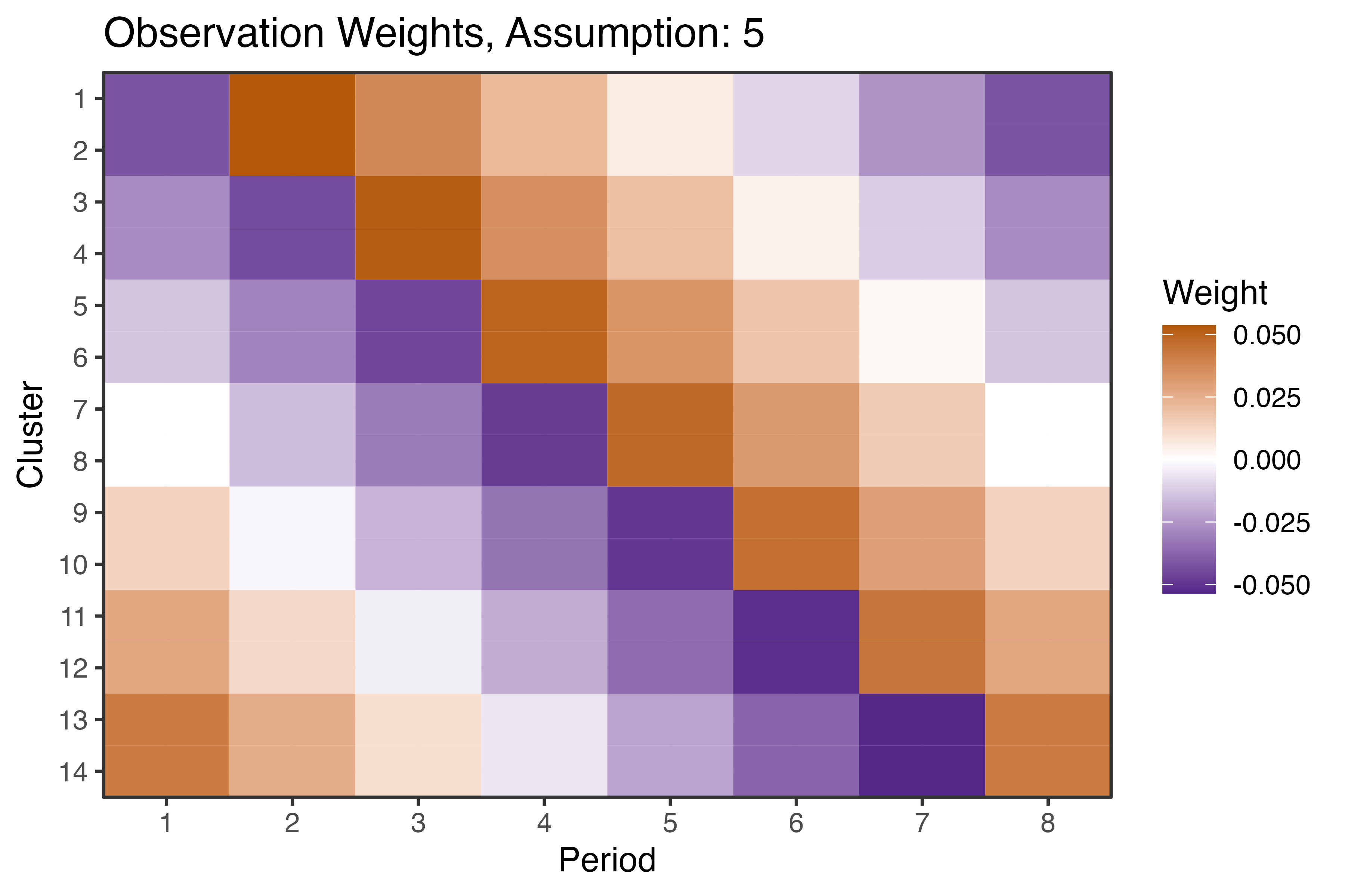
To understand the form of the estimator, we can also examine the weights it gives to each observation (note: the weights to each two-by-two DID estimator are also available, but less interpretable as many different weight vectors can yield the same weights on the observations). The weights for the estimator , again using an exchangeable variance structure, are shown in the heat map in Figure 1. Note that the clusters are ordered by the sequence of treatment adoption, and pairs of clusters (e.g., 1 and 2) have nearly identical weights because they are in the same sequence and assumed to be exchangeable. These weights can be compared to the information content of specific cells under different heterogeneity and correlation assumptions as proposed by Kasza & Forbes (2019) and Kasza, Taljaard & Forbes (2019). Note heurestically that in this case, the largest (in magnitude) weights are near the diagonal, followed by the top-right and bottom-left cells, which are also the highest information-content cells as shown in Figure 4 of Kasza & Forbes (2019).
This method provides flexibility to investigate more specific treatment effects in the heterogeneous settings as well. Considering calendar-time effects under assumption S4, for example, one can estimate the treatment effect in each of months 2 through 7, . For additional robustness against exposure-time heterogeneity, one can also estimate month-specific treatment effects under assumption S2 by averaging across exposure times within each of those months: for all . The estimation and permutation test results on both the multiplicative (odds ratio) and additive (risk difference) scales are shown in Table 4. These results can be compared to the results in Table 2 of Thompson et al. (2018), which reports period-specific risk differences estimated using the purely vertical non-parametric within-period estimator (note that those are labelled by treatment periods, one less than the corresponding month numbers given here). Differences between the methods arise as the results presented here use horizontal information as well, but target the same estimand. Note that no p-values are adjusted for multiple testing.
| Odds Ratio | Risk Difference | |||||||
|---|---|---|---|---|---|---|---|---|
| Assumption S4 | Assumption S2 | Assumption S4 | Assumption S2 | |||||
| Month | Estimate | P-Value | Estimate | P-Value | Estimate | P-Value | Estimate | P-Value |
| 2 | 0.903 | 0.721 | 0.808 | 0.411 | -2.38% | 0.821 | -4.01% | 0.540 |
| 3 | 0.758 | 0.341 | 0.810 | 0.504 | -3.97% | 0.496 | -1.73% | 0.795 |
| 4 | 0.683 | 0.012 | 0.736 | 0.044 | -11.64% | 0.100 | -8.65% | 0.080 |
| 5 | 0.832 | 0.190 | 0.902 | 0.611 | -6.19% | 0.147 | -3.24% | 0.603 |
| 6 | 0.716 | 0.062 | 0.750 | 0.182 | -10.93% | 0.038 | -9.02% | 0.173 |
| 7 | 0.835 | 0.514 | 0.812 | 0.511 | -5.75% | 0.634 | -6.15% | 0.616 |
5 Discussion
The proposed method provides a highly flexible and adaptable approach to analyzing stepped wedge and staggered adoption settings. In particular, it allows the investigator to specify a target estimand that is any linear combination of unique treatment effects and guarantees unbiasedness under the standard assumptions and the particular treatment effect heterogeneity assumptions specified. Among this class of unbiased estimators, the investigator can then identify the one with the lowest variance for an assumed working covariance structure. Analogous to the working correlation matrix used in generalized estimating equations (Zeger & Liang (1986)), this working covariance structure need not be correctly specified to maintain unbiased estimation. A misspecified structure, however, may lead to suboptimal variance and reduced power to detect an effect.
The composition of the estimator from two-by-two DID estimators allows both intuitive connections to methods commonly used in econometrics and quantitative social science for quasi-experimental data as well as assumptions that are familiar to those stepped in that literature. In addition, it allows clear formulation of the treatment effect heterogeneity assumptions that are made rather than those assumptions arising implicitly through a linear regression formulation. By specifying the variance assumption separately, it also removes the need for a correct joint specification of the mean and variance models and allows those assumptions (for the working structure) to be formulated independently of the treatment effect assumptions. These approaches also allow for ease of sensitivity analysis, as the expectation can be found using Equation 5 using a specified weight vector under any other assumption setting. This, along with the potential to assess relative efficiency under the working covariance structure as shown in the example, allows the bias-variance tradeoff to be made explicit, and investigators can consider the appropriate generalizability and interpretation of their target estimands.
In the example re-analyzing the data collected by Trajman et al. (2015), I demonstrated the use of this method for a variety of target estimands in a SWT. Results largely align with those of existing non-parametric estimators, which already had been shown to have desirable bias and inference properties (Thompson et al. (2018); Kennedy‐Shaffer et al. (2020)). In nearly comparable situations, like the assumption of a homogeneous effect compared to the inverse-variance weighted average vertical approach (Thompson et al. (2018)) or either crossover-type estimator (Kennedy‐Shaffer et al. (2020)), this approach had a lower p-value, which may indicate increased power to detect the effect. In addition, many other estimates are tractable using this approach, allowing for flexible pre-specified or exploratory analysis of treatment effect heterogeneity.
Although simulation and testing in other settings are still necessary to determine overall operating characteristics of these estimators, it is reasonable that they are more powerful under homogeneity assumptions than purely vertical approaches since they use horizontal comparisons and than pure crossover approaches since they use information from other comparisons with expectation zero. In addition, the fact that the method generally highly weights cells with high information content (Kasza & Forbes (2019); Kasza, Taljaard & Forbes (2019)) and respects centrosymmetry under appropriate assumptions (Bowden et al. (2021)) indicates efficient use of the observed data. However, their performance compared to regression-based approaches (e.g., Hooper et al. (2016); de Chaisemartin & D’Haultfœuille (2020); Sun & Abraham (2021); Lindner & McConnell (2021); Kenny et al. (2022); Maleyeff et al. (2023); Lee & Cheung (2024)) and existing robust estimators (e.g., Hughes et al. (2020); Callaway & Sant’Anna (2021); Roth & Sant’Anna (2023); Borusyak et al. (2024)) remains to be determined. In particular, future study should determine when this approach provides equivalent estimators to any of those approaches (in particular, those proposed by Sun & Abraham (2021) and Lindner & McConnell (2021)) and under what settings it shows more or less desirable operating characteristics to the others.
Additional future work should consider identifying other approaches to inference, including the possibility of closed-form variance estimators under certain variance assumptions. Identifying appropriate plug-in estimators for use in Equation 10, their robustness to misspecification of the working covariance structure, and the asymptotic distribution would be key, as has been done for mixed effects models with misspecification (see, e.g., Voldal et al. (2022)). This would allow for more targeted design of experiments when analysis will proceed using these methods. Understanding likely covariance structures, especially given planned or conducted approaches for sampling of units (see, e.g., Hooper (2021)), would improve selection of as well. Additionally, modifications of this method to accommodate adjustment for covariates would be useful for non-randomized staggered adoption settings where parallel trends holds only conditionally (see, e.g., Callaway & Sant’Anna (2021); Roth et al. (2023)) and SWTs with restricted, stratified, or matched randomization (see, e.g., Copas et al. (2015)).
Both stepped wedge and staggered adoption settings are common study designs with important roles to play in assessing a variety of policies and implementation approaches; for example, both have been proposed as useful tools for rapid policy evaluation in the COVID-19 pandemic or similar settings (see, e.g., Goodman-Bacon & Marcus (2020); Bell et al. (2021); Cowger et al. (2022); Kennedy-Shaffer (2024)). They each, however, have statistical intricacies that should be carefully considered in the design and analysis (see, e.g., Baker et al. (2022); Nevins et al. (2023)). The generalized DID estimator proposed here has desirable bias and variance properties and interpretability that enable its use across many such settings and desired treatment effect estimands.
Data Availability Statement
All code used for this manuscript is available at https://github.com/leekshaffer/GenDID. Included there is a simulated data set based on this data example. Access policies for the original data set can be found at Trajman et al. (2015), https://doi.org/10.1371/journal.pone.0123252. The author wishes to thank Prof. Anete Trajman for making the data available to the author for re-analysis and Prof. Jennifer Thompson for helpful discussions regarding the data.
References
- (1)
-
Athey & Imbens (2022)
Athey, S. & Imbens, G. W. (2022),
‘Design-based analysis in difference-in-differences settings with staggered
adoption’, Journal of Econometrics 226(1), 62–79.
https://doi.org/10.1016/j.jeconom.2020.10.012 -
Baker et al. (2022)
Baker, A. C., Larcker, D. F. & Wang, C. C. (2022), ‘How much should we trust staggered
difference-in-differences estimates?’, Journal of Financial Economics
144(2), 370–395.
https://doi.org/10.1016/j.jfineco.2022.01.004 -
Bell et al. (2021)
Bell, K. J. L., Glasziou, P., Stanaway, F., Bossuyt, P. & Irwig, L.
(2021), ‘Equity and evidence during vaccine
rollout: stepped wedge cluster randomised trials could help’, BMJ 372, n435.
https://doi.org/10.1136/bmj.n435 -
Borusyak et al. (2024)
Borusyak, K., Jaravel, X. & Spiess, J. (2024), ‘Revisiting event study designs: Robust and
efficient estimation’.
arXiv:2108.12419 [econ].
http://arxiv.org/abs/2108.12419 -
Bowden et al. (2021)
Bowden, R., Forbes, A. B. & Kasza, J. (2021), ‘On the centrosymmetry of treatment effect estimators
for stepped wedge and related cluster randomized trial designs’, Statistics & Probability Letters 172, 109022.
https://doi.org/10.1016/j.spl.2020.109022 -
Callaway & Sant’Anna (2021)
Callaway, B. & Sant’Anna, P. H. (2021), ‘Difference-in-differences with multiple time
periods’, Journal of Econometrics 225(2), 200–230.
https://doi.org/10.1016/j.jeconom.2020.12.001 -
Copas et al. (2015)
Copas, A. J., Lewis, J. J., Thompson, J. A., Davey, C., Baio, G. & Hargreaves, J. R. (2015), ‘Designing a
stepped wedge trial: three main designs, carry-over effects and randomisation
approaches’, Trials 16(1), 352.
https://doi.org/10.1186/s13063-015-0842-7 -
Cowger et al. (2022)
Cowger, T. L., Murray, E. J., Clarke, J., Bassett, M. T., Ojikutu, B. O.,
Sánchez, S. M., Linos, N. & Hall, K. T. (2022), ‘Lifting universal masking in schools — Covid-19
incidence among students and staff’, New England Journal of Medicine
387(21), 1935–1946.
https://doi.org/10.1056/NEJMoa2211029 - Cunningham (2021) Cunningham, S. (2021), Causal Inference: The Mixtape, Yale University Press, New Haven, CT.
-
de Chaisemartin & D’Haultfœuille (2020)
de Chaisemartin, C. & D’Haultfœuille, X. (2020), ‘Two-way fixed effects estimators with heterogeneous
treatment effects’, American Economic Review 110(9), 2964–2996.
https://doi.org/10.1257/aer.20181169 -
de Chaisemartin & D’Haultfœuille (2023)
de Chaisemartin, C. & D’Haultfœuille, X. (2023), ‘Two-way fixed effects and differences-in-differences
with heterogeneous treatment effects: a survey’, The Econometrics
Journal 26(3), C1–C30.
https://doi.org/10.1093/ectj/utac017 -
Durovni et al. (2014)
Durovni, B., Saraceni, V., Van Den Hof, S., Trajman, A., Cordeiro-Santos, M.,
Cavalcante, S., Menezes, A. & Cobelens, F. (2014), ‘Impact of replacing smear microscopy with Xpert
MTB/RIF for diagnosing tuberculosis in Brazil: A stepped-wedge
cluster-randomized trial’, PLoS Medicine 11(12), e1001766.
https://doi.org/10.1371/journal.pmed.1001766 - George & Ajayakumar (2024) George, R. K. & Ajayakumar, A. (2024), A Course in Linear Algebra, Springer, Singapore.
-
Goodman-Bacon (2021)
Goodman-Bacon, A. (2021),
‘Difference-in-differences with variation in treatment timing’, Journal
of Econometrics 225(2), 254–277.
https://doi.org/10.1016/j.jeconom.2021.03.014 -
Goodman-Bacon & Marcus (2020)
Goodman-Bacon, A. & Marcus, J. (2020), ‘Using difference-in-differences to identify causal
effects of COVID-19 policies’, Survey Research Methods 14(2), 153–158.
https://doi.org/10.18148/SRM/2020.V14I2.7723 -
Hagemann (2019)
Hagemann, A. (2019), ‘Placebo inference on
treatment effects when the number of clusters is small’, Journal of
Econometrics 213(1), 190–209.
https://doi.org/10.1016/j.jeconom.2019.04.011 -
Hooper (2021)
Hooper, R. (2021), ‘Key concepts in clinical
epidemiology: Stepped wedge trials’, Journal of Clinical Epidemiology
137, 159–162.
https://linkinghub.elsevier.com/retrieve/pii/S0895435621001190 -
Hooper et al. (2016)
Hooper, R., Teerenstra, S., De Hoop, E. & Eldridge, S.
(2016), ‘Sample size calculation for stepped
wedge and other longitudinal cluster randomised trials: Sample size
calculation for stepped wedge trials’, Statistics in Medicine 35(26), 4718–4728.
https://doi.org/10.1002/sim.7028 -
Hughes et al. (2020)
Hughes, J. P., Heagerty, P. J., Xia, F. & Ren, Y. (2020), ‘Robust inference for the stepped wedge design’, Biometrics 76(1), 119–130.
https://doi.org/10.1111/biom.13106 -
Imai & Kim (2021)
Imai, K. & Kim, I. S. (2021), ‘On
the use of two-way fixed effects regression models for causal inference with
panel data’, Political Analysis 29(3), 405–415.
https://doi.org/10.1017/pan.2020.33 -
Kahn-Lang & Lang (2020)
Kahn-Lang, A. & Lang, K. (2020),
‘The promise and pitfalls of differences-in-differences: Reflections on
16 and Pregnant and other applications’, Journal of Business
& Economic Statistics 38(3), 613–620.
https://doi.org/10.1080/07350015.2018.1546591 -
Kasza & Forbes (2019)
Kasza, J. & Forbes, A. B. (2019),
‘Information content of cluster–period cells in stepped wedge trials’, Biometrics 75(1), 144–152.
https://doi.org/10.1111/biom.12959 -
Kasza, Hemming, Hooper, Matthews & Forbes (2019)
Kasza, J., Hemming, K., Hooper, R., Matthews, J. & Forbes, A.
(2019), ‘Impact of non-uniform correlation
structure on sample size and power in multiple-period cluster randomised
trials’, Statistical Methods in Medical Research 28(3), 703–716.
https://doi.org/10.1177/0962280217734981 -
Kasza, Taljaard & Forbes (2019)
Kasza, J., Taljaard, M. & Forbes, A. B. (2019), ‘Information content of stepped‐wedge designs when
treatment effect heterogeneity and/or implementation periods are present’,
Statistics in Medicine 38(23), 4686–4701.
https://doi.org/10.1002/sim.8327 -
Kennedy-Shaffer (2024)
Kennedy-Shaffer, L. (2024),
‘Quasi-experimental methods for pharmacoepidemiology:
difference-in-differences and synthetic control methods with case studies for
vaccine evaluation’, American Journal of Epidemiology
(10.1093/aje/kwae019).
https://doi.org/10.1093/aje/kwae019 -
Kennedy-Shaffer & Lipsitch (2020)
Kennedy-Shaffer, L. & Lipsitch, M. (2020), ‘Statistical properties of stepped wedge
cluster-randomized trials in infectious disease outbreaks’, American
Journal of Epidemiology 189(11), 1324–1332.
https://doi.org/10.1093/aje/kwaa141 -
Kennedy‐Shaffer et al. (2020)
Kennedy‐Shaffer, L., De Gruttola, V. & Lipsitch, M.
(2020), ‘Novel methods for the analysis of
stepped wedge cluster randomized trials’, Statistics in Medicine 39(7), 815–844.
https://doi.org/10.1002/sim.8451 -
Kenny et al. (2022)
Kenny, A., Voldal, E. C., Xia, F., Heagerty, P. J. & Hughes, J. P.
(2022), ‘Analysis of stepped wedge cluster
randomized trials in the presence of a time‐varying treatment effect’, Statistics in Medicine 41(22), 4311–4339.
https://doi.org/10.1002/sim.9511 -
Lee & Cheung (2024)
Lee, K. M. & Cheung, Y. B. (2024),
‘Cluster randomized trial designs for modeling time‐varying intervention
effects’, Statistics in Medicine 43(1), 49–60.
https://doi.org/10.1002/sim.9941 -
Li et al. (2023)
Li, F., Chen, X., Tian, Z., Wang, R. & Heagerty, P. J.
(2023), ‘Planning stepped wedge cluster
randomized trials to detect treatment effect heterogeneity’, Statistics
in Medicine (10.1002/sim.9990).
https://doi.org/10.1002/sim.9990 -
Lindner & McConnell (2021)
Lindner, S. & McConnell, K. J. (2021), ‘Heterogeneous treatment effects and bias in the
analysis of the stepped wedge design’, Health Services and Outcomes
Research Methodology 21(4), 419–438.
https://doi.org/10.1007/s10742-021-00244-w -
MacKinnon & Webb (2020)
MacKinnon, J. G. & Webb, M. D. (2020), ‘Randomization inference for
difference-in-differences with few treated clusters’, Journal of
Econometrics 218(2), 435–450.
https://doi.org/10.1016/j.jeconom.2020.04.024 -
Maleyeff et al. (2023)
Maleyeff, L., Li, F., Haneuse, S. & Wang, R. (2023), ‘Assessing exposure-time treatment effect
heterogeneity in stepped-wedge cluster randomized trials’, Biometrics
79(3), 2551–2564.
https://doi.org/10.1111/biom.13803 -
Matthews & Forbes (2017)
Matthews, J. N. S. & Forbes, A. B. (2017), ‘Stepped wedge designs: Insights from a design of
experiments perspective’, Statistics in Medicine 36(24), 3772–3790.
https://doi.org/10.1002/sim.7403 -
Nevins et al. (2023)
Nevins, P., Ryan, M., Davis-Plourde, K., Ouyang, Y., Pereira Macedo, J. A.,
Meng, C., Tong, G., Wang, X., Ortiz-Reyes, L., Caille, A., Li, F.
& Taljaard, M. (2023),
‘Adherence to key recommendations for design and analysis of stepped-wedge
cluster randomized trials: A review of trials published 2016–2022’, Clinical Trials (10.1177/17407745231208397).
https://doi.org/10.1177/17407745231208397 -
Nickless et al. (2018)
Nickless, A., Voysey, M., Geddes, J., Yu, L.-M. & Fanshawe, T. R.
(2018), ‘Mixed effects approach to the
analysis of the stepped wedge cluster randomised trial—Investigating the
confounding effect of time through simulation’, PLOS ONE 13(12), e0208876.
https://doi.org/10.1371/journal.pone.0208876 -
Roth et al. (2023)
Roth, J., Sant’Anna, P. H., Bilinski, A. & Poe, J.
(2023), ‘What’s trending in
difference-in-differences? A synthesis of the recent econometrics
literature’, Journal of Econometrics 235(2), 2218–2244.
https://doi.org/10.1016/j.jeconom.2023.03.008 -
Roth & Sant’Anna (2023)
Roth, J. & Sant’Anna, P. H. C. (2023), ‘Efficient estimation for staggered rollout designs’,
Journal of Political Economy Microeconomics 1(4), 669–709.
https://doi.org/10.1086/726581 -
Shaikh & Toulis (2021)
Shaikh, A. M. & Toulis, P. (2021),
‘Randomization tests in observational studies With staggered adoption of
treatment’, Journal of the American Statistical Association 116(536), 1835–1848.
https://doi.org/10.1080/01621459.2021.1974458 -
Sun & Abraham (2021)
Sun, L. & Abraham, S. (2021),
‘Estimating dynamic treatment effects in event studies with heterogeneous
treatment effects’, Journal of Econometrics 225(2), 175–199.
https://doi.org/10.1016/j.jeconom.2020.09.006 -
Thompson et al. (2018)
Thompson, J., Davey, C., Fielding, K., Hargreaves, J. & Hayes, R.
(2018), ‘Robust analysis of stepped wedge
trials using cluster‐level summaries within periods’, Statistics in
Medicine 37(16), 2487–2500.
https://doi.org/10.1002/sim.7668 -
Trajman et al. (2015)
Trajman, A., Durovni, B., Saraceni, V., Menezes, A., Cordeiro-Santos, M.,
Cobelens, F. & Van Den Hof, S. (2015), ‘Impact on patients’ treatment outcomes of
XpertMTB/RIF implementation for the diagnosis of tuberculosis:
Follow-up of a stepped-wedge randomized clinical trial’, PLOS ONE
10(4), e0123252.
https://doi.org/10.1371/journal.pone.0123252 -
Twisk et al. (2016)
Twisk, J., Hoogendijk, E., Zwijsen, S. & De Boer, M.
(2016), ‘Different methods to analyze
stepped wedge trial designs revealed different aspects of intervention
effects’, Journal of Clinical Epidemiology 72, 75–83.
https://doi.org/10.1016/j.jclinepi.2015.11.004 -
Voldal et al. (2022)
Voldal, E. C., Xia, F., Kenny, A., Heagerty, P. J. & Hughes, J. P.
(2022), ‘Model misspecification in stepped
wedge trials: Random effects for time or treatment’, Statistics in
Medicine 41(10), 1751–1766.
https://doi.org/10.1002/sim.9326 -
Wang & De Gruttola (2017)
Wang, R. & De Gruttola, V. (2017), ‘The use of permutation tests for the analysis of parallel and
stepped‐wedge cluster‐randomized trials’, Statistics in Medicine
36(18), 2831–2843.
https://doi.org/10.1002/sim.7329 -
Zeger & Liang (1986)
Zeger, S. L. & Liang, K.-Y. (1986), ‘Longitudinal data analysis for discrete and continuous outcomes’, Biometrics 42(1), 121–130.
https://doi.org/10.2307/2531248
APPENDICES
Appendix A Determining the Matrix of DID Estimators
For any integer , define as the matrix where:
where is the column vector of 1’s and is the identity matrix.
Now define for a setting with time periods as the matrix given by:
where is the column vector of 0’s.
Finally, define for a setting with time periods and clusters as the matrix given by:
where is the matrix of 0’s. Note that, in the above representation, each row represents rows. In each of these, columns are from matrices, while the other are from two copies of the matrix.
This is the matrix that, when multiplied (on the right) by the column vector of outcomes , gives the column vector of two-by-two DID estimators . In particular, will be found on the following row number of the vector :
Conversely, row in the vector , for , corresponds to the two-by-two DID estimator where the indices are given by the following algorithm:
-
1.
Let and
-
2.
Let be the minimum such that . Then and .
-
3.
Let be the minimum such that . Then and .
Each row can then be associated with the corresponding . From the values of and , along with and , the type (from 1–6) of this two-by-two DID estimator can then be determined. And its expectation under the desired assumption setting can be determined as well. Thus, the column vector and associated matrix can be constructed in terms of the estimands possible for the assumption setting.
Appendix B Proofs of Key Lemmata and Theorems
B.1 Lemmata for Proof of Theorem 3
Lemma 4 Let and be as defined previously. Then .
Proof. Let ; that is, . Then for any . Since this is true for any , it must be true in expectation, so . For this to be true for any vector of treatment effects, then, and . So , as desired.
Lemma 5 Let be as defined previously for a setting with units and periods. Then .
Proof. For any , , let be the row of corresponding to (i.e., ). has the value 1 in the columns corresponding to and , -1 in the columns corresponding to and , and 0 in all other columns.
Consider the matrix composed of only the rows of the form of , where and . This is a matrix. Any row can be expressed as a linear combination of the rows of as follows:
Thus, . Moreover, the rows of are linearly independent, since each row of the form is the unique row of that form to have a non-zero entry in the column corresponding to . So . Since is a real matrix, as well.
B.2 Proof of Theorem 3
Theorem 3 Let , , , and be as defined previously. Then the following are true about the set of estimators of the form that are unbiased for under the assumption setting:
-
•
If , then there are no estimators of this form that are unbiased for .
-
•
If , then there is a unique estimator of this form that is unbiased for , defined by the unique that solves .
-
•
If , then there are infinitely many estimators of this form that are unbiased for . The dimension of unique such estimators is .
Proof. By results on non-homogeneous systems of linear equations (also known as the Rouché-Capelli Theorem; see George & Ajayakumar (2024), p. 41) on the equation , there are two possibilities:
-
•
If , then there are no solutions.
-
•
If , then there is a solution to the system, and the affine space of solutions has dimension , since is of dimension , where is the number of unique treatment effects.
If , then, there is a single unique solution , which corresponds to a single unique estimator of the desired form that is unbiased for .
If , there are infinitely many solutions . Two distinct solutions , however, may correspond to the same estimator , since different weightings of the two-by-two DID estimators may result in the same weightings of the underlying observations.
Let be a solution to . Any other solution to can be expressed as , where . The vector space of has dimension , corresponding to the dimension of the affine space as found above. By Lemma 4, , and so can be written as the direct sum of , where is defined as the orthogonal complement of within . So we can further express . However, if . Hence, for any and any , , and so the estimators and defined by the weight vectors and are equal for all . Thus, the only unique estimators (in terms of the underlying observations) are given by the subspace .
Appendix C Supplementary Results
| Exchangeable, | AR(1), | ||||||
|---|---|---|---|---|---|---|---|
| Independence | |||||||
| Assumption | Estimator | Estimate | P-Value | Estimate | P-Value | Estimate | P-Value |
| S5 | 0.771 | 0.014 | 0.771 | 0.009 | 0.772 | 0.012 | |
| S4 | 0.784 | 0.024 | 0.784 | 0.031 | 0.785 | 0.029 | |
| S3 | 0.828 | 0.391 | 0.828 | 0.397 | 0.827 | 0.364 | |
| S2 | 0.801 | 0.168 | 0.801 | 0.160 | 0.802 | 0.160 | |
| Exchangeable, | AR(1), | ||||||
|---|---|---|---|---|---|---|---|
| Independence | |||||||
| Assumption | Estimator | Estimate | P-Value | Estimate | P-Value | Estimate | P-Value |
| S5 | -7.35% | 0.020 | -7.35% | 0.015 | -7.33% | 0.024 | |
| S4 | -6.81% | 0.039 | -6.81% | 0.052 | -6.78% | 0.045 | |
| S3 | -5.57% | 0.430 | -5.57% | 0.423 | -5.58% | 0.411 | |
| S2 | -6.11% | 0.240 | -6.11% | 0.243 | -6.09% | 0.230 | |