Addressing Misspecification in Simulation-based Inference through Data-driven Calibration

Abstract

Driven by steady progress in generative modeling, simulation-based inference (SBI) has enabled inference over stochastic simulators. However, recent work has demonstrated that model misspecification can harm SBI’s reliability. This work introduces robust posterior estimation (ROPE), a framework that overcomes model misspecification with a small real-world calibration set of ground truth parameter measurements. We formalize the misspecification gap as the solution of an optimal transport problem between learned representations of real-world and simulated observations. Assuming the prior distribution over the parameters of interest is known and well-specified, our method offers a controllable balance between calibrated uncertainty and informative inference under all possible misspecifications of the simulator. Our empirical results on four synthetic tasks and two real-world problems demonstrate that ROPE outperforms baselines and consistently returns informative and calibrated credible intervals.

1 Introduction

Many fields of science and engineering have shifted in recent years from modeling real-world phenomena through a few equations to relying instead on highly complex computer simulations. While this shift has increased model versatility and the ability to explain complex phenomena, it has also necessitated the development of new statistical inference methods. In particular, state-of-the-art simulation-based inference (SBI, Cranmer et al.,, 2020) algorithms leverage neural networks to learn surrogate models of the likelihood (Papamakarios et al.,, 2019), likelihood ratio (Hermans et al.,, 2020), or posterior distribution (Papamakarios and Murray,, 2016), from which one can extract confidence or credible intervals over the parameters of interest given an observation. While SBI has proven helpful when the simulator is a faithful description of the studied phenomenon, e.g., for scientific applications (Delaunoy et al.,, 2020; Brehmer,, 2021; Lückmann,, 2022; Linhart et al.,, 2022; Hashemi et al.,, 2022; Tolley et al.,, 2023; Avecilla et al.,, 2022), recent work has highlighted the unreliability of SBI methods under model misspecification (Cannon et al.,, 2022; Rodrigues et al.,, 2022).

Misspecification in SBI.

A model is a simplified description of a real-world phenomenon that allows reasoning about its properties. Thus, model misspecification arises in a context where the validity of simplifying assumptions cannot be totally verified. In the Bayesian inference literature (Walker,, 2013), a statistical model $p(\mathbf{x}_{s}\mid\theta)$ that relates a parameter of interest $\theta\in\Theta$ to a conditional distribution over simulated observations $\mathbf{x}_{s}$ is said to be misspecified if the true data generating process $p^{\star}(\mathbf{x}_{o})$ of the real observations $\mathbf{x}_{o}\sim p^{\star}(\mathbf{x}_{o})$ does not fall within the family of distributions defined by the model, i.e. $\nexists\theta\in\Theta:p^{\star}(\mathbf{x}_{o})=p(\mathbf{x}_{o}\mid\theta)$. Based on this definition, Ward et al., (2022); Huang et al., (2023) have investigated solutions to improve the robustness of existing SBI algorithms to misspecified models. Here, we depart slightly from this definition of misspecification and instead tailor it to Bayesian uncertainty quantification, in particular, the prediction of credible regions on the parameter $\theta$ given an observation $\mathbf{x}_{o}$. We assume real-world data are sampled i.i.d. from the distribution $p^{\star}(\mathbf{x}_{o}):=\int p(\theta)p^{\star}(\mathbf{x}_{o}\mid\theta)d\theta$, where $p(\theta)$ is a known prior over the parameter we aim to infer and $p^{\star}(\mathbf{x}_{o}\mid\theta)$ is an unknown process approximated by a simulator that generates simulations $\mathbf{x}_{s}\sim p(\mathbf{x}_{s}\mid\theta)$ given a parameter $\theta$. We say the simulator is misspecified if there exists at least an observation $\mathbf{x}_{o}$ for which the simulator posterior $p(\theta\mid\mathbf{x}_{o})\neq p^{\star}(\theta\mid\mathbf{x}_{o})$, where $p^{\star}(\theta\mid\mathbf{x}_{o}):=\frac{p(\theta)p^{\star}(\mathbf{x}_{o}\mid\theta)}{p^{\star}(\mathbf{x}_{o})}$. Notably, our definition can be interpreted as a generalized definition of miss-calibration and encompasses the definition of misspecification used in the Bayesian inference literature as a special case. While such miss-calibration often arises in practical settings where the simulator does not faithfully model some aspects of the true generating process, current SBI algorithms and their robust version may fail drastically.

Addressing Misspecification with a Calibration Set

In this work, we address model misspecification through a calibration set consisting of only a few pairs of real-world observations and their corresponding ground-truth labels. At first glance, having access to a calibration set may seem like an assumption that limits the applicability of such an approach. On the contrary, we argue that for any real-world task where the output of the inference is itself to be trusted, e.g., to monitor a parameter in a critical process, we will likely have access to a calibration set as obtained, for example, through a more costly procedure or measurement device. Indeed, unless we can confidently place additional assumptions on the form of the misspecification–a difficult task, since it is by definition unknown–the only way to validate the inference directly is through a validation set consisting of real-world observations and their ground-truth labels. If such a set exists, we can take a few observations to form our calibration set.

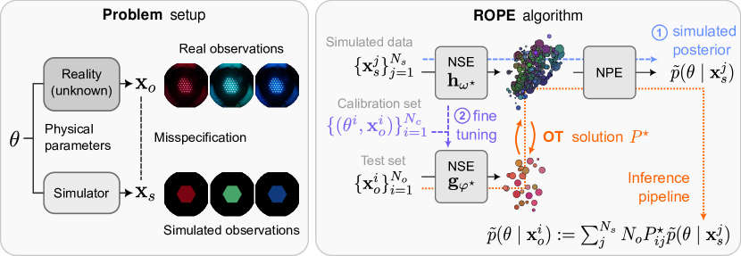
Figure 1: (left) Problem setup: we consider a real-world process which depends on some physical parameters $\theta$. Given real observations $\mathbf{x}_{o}$ of the process, our goal is to provide uncertainty quantification on the underlying parameters $\theta$. To help us, we have access to a misspecified simulator that takes parameters $\theta$ as input and produces simulated observations $\mathbf{x}_{s}$. (right) A visualization of ROPE. The training consists of two steps: (1) We approximate the posterior given the simulated data using NPE, resulting in the NSE $\mathbf{h}_{\omega^{\star}}$. (2) Using the calibration set, we fine-tune $\mathbf{h}_{\omega^{\star}}$ into $\mathbf{g}_{\varphi^{\star}}$ using the objective (7). At test time, we solve the OT problem between the representations $\{\mathbf{h}_{\omega^{\star}}(\mathbf{x}_{s}^{j})\}_{j=1}^{N_{s}}$ and $\{\mathbf{g}_{\varphi^{\star}}(\mathbf{x}_{o}^{i})\}_{i=1}^{N_{o}}$, resulting in our estimated posterior (6): the average of simulations’ posteriors weighted by the OT solution $P^{\star}$. See 21 for more details.

Our Contributions.

We introduce robust posterior estimation (ROPE), an algorithm that overcomes model misspecification to provide accurate uncertainty quantification for the parameters of stochastic and non-differentiable simulators. To achieve this, ROPE relies on (1) a correctly defined prior, and (2) having access to a small, real-world calibration set of paired parameters and observations. The algorithm extends neural posterior estimation Papamakarios and Murray, (2016) with optimal transport (OT, Peyré et al.,, 2017; Villani et al.,, 2009) to model the misspecification as an OT coupling between simulated and real-world data. We evaluate the performance of the algorithm on existing benchmarks from the SBI literature, and introduce four new benchmarks, of which two are synthetic and two come from real physical systems for which both labeled data and simulators are available. To the best of our knowledge, the latter constitute the first real-world benchmarks for SBI under misspecified models. We also perform experiments to explore the effect different calibration set sizes have on the performance of the algorithm, together with ablation studies to understand the impact of each of its components.

2 Background & Notations

In this section, we provide a short review of SBI and OT, as our method is at the intersection of these two fields. We start with some more fundamental definitions. We consider a simulator, implemented as a computer program $S:\mathbb{R}^{K}\times[0,1]\rightarrow\mathbb{R}^{D}$, that takes in physical parameters $\theta\in\Theta\subseteq\mathbb{R}^{K}$ and a random seed $\varepsilon\in[0,1]$ to generate measurements $\mathbf{x}_{s}\in\mathcal{X}_{s}\subseteq\mathbb{R}^{D}$. The simulator is a simplified version of a real and unknown generative process $p^{\star}(\mathbf{x}_{o})$ that produces real-world observations $\mathbf{x}_{o}\in\mathcal{X}_{o}\subseteq\mathbb{R}^{D}$. We assume this process depends on parameters with the same physical meaning as the ones of the simulator and thus use the same notation $\theta$. Our goal is to estimate a well-calibrated and informative posterior distribution $p(\theta\mid\mathbf{x}^{i}_{o})$ for each observation in the test set $\mathbf{x}^{i}_{o}\in\mathcal{D}$, which reduces uncertainty compared to the prior distribution. As a remark, the most informative and calibrated posterior is the Bayesian posterior $p^{\star}(\theta\mid\mathbf{x}_{o})$ that corresponds to true generative process $p^{\star}(\mathbf{x}_{o}):=\int p^{\star}(\mathbf{x}_{o}\mid\theta)p(\theta)\text{d}\theta$. To achieve our goal, we have access to (a) the misspecified simulator $S$ that embeds domain knowledge and approximates $p^{\star}(\mathbf{x}_{o}\mid\theta)$, (b) a small calibration set of labeled real-world observations $\mathcal{C}:=\{(\theta^{i},\mathbf{x}_{o}^{i})\}_{i=1}^{N_{c}}$, which enables data-driven correction of the simulator’s misspecification, and (c) a test set $\mathcal{D}:=\{\mathbf{x}_{o}^{i}\}_{i=1}^{N_{o}}$ of real-world observations arising from $p^{\star}(\mathbf{x}_{o})$ for which we want to estimate the posterior.

2.1 Simulation-based Inference (SBI)

Applying statistical inference to simulators is challenged by the absence of a tractable likelihood function (Cranmer et al.,, 2020). As a solution, SBI algorithms leverage modern machine learning methods to tackle inference in this likelihood-free setting (Lueckmann et al.,, 2021; Delaunoy et al.,, 2021; Glöckler et al.,, 2022). Among SBI algorithms, neural posterior estimation NPE (Papamakarios and Murray,, 2016; Lueckmann et al.,, 2017) is a broadly applicable method that trains a conditional density estimator of $p(\theta\mid\mathbf{x}_{s})$ from a dataset of parameter-simulation pairs. In this paper, we focus on making NPE robust to model misspecification.

NPE usually parametrizes the posterior with a neural conditional density estimator (NCDE), which is composed of (1) a neural statistic estimator (NSE), denoted by $\mathbf{h}_{\omega}:\mathcal{X}_{s}\rightarrow\mathbb{R}^{l}$, that compresses observations into $l\text{-dimensional}$ representations and, (2) a normalizing flow (NF, Papamakarios et al.,, 2021; Tabak and Vanden-Eijnden,, 2010) that parameterizes the posterior density as $p_{\phi}(\theta\mid\mathbf{h}_{\omega}(\mathbf{x}_{s}))$. The parameters $\phi$ and $\omega$ of the NCDE are trained with stochastic gradient ascent on the expected log-posterior probability, solving the following optimization problem

$$\phi^{\star},\omega^{\star}= \arg\max_{\phi,\omega}\mathbb{E}_{\begin{subarray}{c}\theta\sim p(\theta)\\ \varepsilon\sim\mathcal{U}[0,1]\end{subarray}}\left[\log p_{\phi}(\theta\mid\mathbf{h}_{\omega}(S(\theta,\varepsilon)))\right],$$ (1)

where $p(\theta)$ denotes a prior distribution over the parameters $\theta$.

Under the assumption that the class of functions represented by the NCDE contains the true posterior, solving (1) leads to a perfect surrogate $p_{\phi^{\star}}(\theta\mid\mathbf{h}_{\omega^{\star}}(\mathbf{x}_{s}))$ of the true posterior $p(\theta\mid\mathbf{x}_{s})$. In that case, $\theta\perp\mathbf{x}_{s}\mid\mathbf{h}_{\omega^{\star}}(\mathbf{x}_{s})$, that is, the NSE $\mathbf{h}_{\omega^{\star}}$ is a sufficient statistic of $\mathbf{x}_{s}$ for the parameter $\theta$. In practice, we approach perfect training by generating a sufficiently large number of pairs $(\theta,\mathbf{x}_{s})$ and doing a search on the NCDE’s architecture and training hyperparameters. As we will see in Section 3, NPE and the sufficiency of the NSE are at the root of our algorithm. To simplify notation, we denote the NCDE learned with NPE as $\tilde{p}(\theta\mid\mathbf{x}_{s})$

2.2 Optimal Transport (OT)

As detailed in Section 3, our algorithm models the misspecification between simulations and real-world observations as an OT coupling. In particular, let $p(\mathbf{x}_{o})$ and $p(\mathbf{x}_{s})$ be two continuous probability measures in $\mathcal{X}_{o}$ and $\mathcal{X}_{s}$, respectively, and consider a cost function $c:\mathcal{X}_{o}\times\mathcal{X}_{s}\rightarrow\mathbb{R}$ that assigns a cost to each pair $(\mathbf{x}_{o},\mathbf{x}_{s})\in\mathcal{X}_{o}\times\mathcal{X}_{s}$. Then, we wish to find the OT coupling

$$\pi^{\star}=\arg\min_{\pi\in\Pi}\mathbb{E}_{\pi}[c(\mathbf{x}_{o},\mathbf{x}_{s})],$$ (2)

where $\Pi$ is the set of joint probability measures on $\mathcal{X}_{o}\times\mathcal{X}_{s}$ whose marginals are $p(\mathbf{x}_{o})$ and $p(\mathbf{x}_{s})$.

In our setting, we only have access to a limited number $N_{o}$ of real-world observations $\{\mathbf{x}_{o}^{i}\}_{i=1}^{N_{o}}$, which we assume result from an unknown generative $p^{\star}(\mathbf{x}_{o})=\int p^{\star}(\mathbf{x}_{o}\mid\theta)p(\theta)\text{d}\theta$. Thus, we solve the discrete and entropy-regularized version of (2). Namely, given a set $\{\mathbf{x}_{s}^{j}\}_{j=1}^{N_{s}}$ of simulated observations, we search for the doubly stochastic transport matrix $P^{\star}$, in the polytope of transport couplings $\mathcal{B}\!:=\{P\in\mathbb{R}^{N_{o}\times N_{s}}_{+}:P\mathbf{1}_{N_{s}}=\mathbf{1}_{N_{o}}/N_{o},P^{T}\mathbf{1}_{N_{o}}=\mathbf{1}_{N_{s}}/N_{s}\},$ that solves

$$P^{\star}=\arg\min_{P\in\mathcal{B}}\sum_{ij}^{N_{o}\times N_{s}}P_{ij}\left(c(\mathbf{x}_{o}^{i},\mathbf{x}_{s}^{j})+\gamma\log P_{ij}\right),$$ (3)

where $\gamma>0$ can be seen as a hyperparameter that encourages entropic transport matrices. The entropy-regularized transport problem can be solved with the Sinkhorn algorithm (Cuturi,, 2013), which is a fixed-point iteration algorithm with an efficient GPU implementation. In our experiments, we rely on the OTT (Cuturi et al.,, 2022) implementation of Sinkhorn, which returns the transport coupling $P^{\star}$ given the cost matrix $C:C_{ij}=c(\mathbf{x}_{o}^{i},\mathbf{x}_{s}^{j})$ and the entropic regularization factor $\gamma$.

3 Modeling Misspecification with OT

We approach the problem of misspecification as a modeling task rather than seeing it as an issue of the inference algorithm. As our main modeling assumption, we assume that

$$\mathbf{x}_{o}\perp\theta\mid\mathbf{x}_{s},$$ (4)

that is, given the simulated observations $\mathbf{x}_{s}$, the real observations $\mathbf{x}_{o}$ contain no additional information about the parameters $\theta$.

While this assumption allows us to express the misspecification independently from $\theta$, it might be violated in practice, as is the case for the two real physical systems we study in section 4. Due to the construction of our algorithm, violations do not prevent obtaining calibrated and informative posterior distributions. However, the assumption may limit uncertainty reduction by preventing our method from exploiting any signal in the real data beyond what is specified by the simulator. This can be a limiting factor for highly misspecified simulators, but if the simulator encodes phenomena that the practitioner believes are invariant across different application environments, the assumption can also prevent shortcut learning from the calibration data and benefit the generalization of the method. In Appendix A, we evaluate the method on real out-of-distribution data and demonstrate this property.

The OT coupling in (2) fulfills the definition of a joint distribution in $\mathcal{X}_{o}\times\mathcal{X}_{s}$, and together with our modelling assumption (4), we can express the posterior distribution for real-world observations as

$$p(\theta\mid\mathbf{x}_{o})=\int p(\theta\mid\mathbf{x}_{s})\pi^{\star}(\mathbf{x}_{s}\mid\mathbf{x}_{o})d\mathbf{x}_{s},$$ (5)

where the simulation posterior $p(\theta\mid\mathbf{x}_{s})$ can be approximated arbitrarily well with NPE (Papamakarios and Murray,, 2016), as NFs are universal density estimators of continuous distributions (Wehenkel and Louppe,, 2019).

Motivated by the factorization in (5), our algorithm computes a transport matrix $P^{\star}$ between the test set $\mathcal{D}$ and a set $\{\mathbf{x}^{j}_{s}\}_{j=1}^{N_{s}}$ of $N_{s}$ simulations generated by running the simulator on parameters from the prior $\theta^{j}\sim p(\theta)$. Thus, approximating (5), we estimate the posterior for real-world observations as a mixture of posteriors $\tilde{p}$ obtained with NPE, that is,

$$\tilde{p}(\theta\mid\mathbf{x}_{o}^{i}):=\sum_{j}^{N_{s}}\alpha_{ij}\tilde{p}(\theta\mid\mathbf{x}^{j}_{s}),\text{ where }\alpha_{ij}=N_{o}P^{\star}_{ij}.$$ (6)

An interesting property of defining ROPE as in $\eqref{eq:real_posterior_def}$ is that, by design, the marginal posterior distribution over the test set, i.e., $\tilde{p}(\theta):=\int\tilde{p}(\theta\mid\mathbf{x}_{o})p^{\star}(\mathbf{x}_{o})\text{d}\mathbf{x}_{o}$, converges to the prior distribution as the number of simulated observations $N_{s}$ approaches infinity, as expected from a well-estimated posterior distribution. A proof and further discussion of this self-calibration property is given in Appendix B.

3.1 Defining the OT Cost Function

In our context, an ideal coupling would assign simulations to real-world observations generated from the same parameter. Hence, we can express the corresponding ideal cost as $c(\mathbf{x}_{o},\mathbf{x}_{s})=c(\mathbf{h}_{o}(\mathbf{x}_{o}),\mathbf{h}_{s}(\mathbf{x}_{s}))$, where $\mathbf{h}_{o}$ and $\mathbf{h}_{s}$ are any sufficient statistics for $\theta$ given $\mathbf{x}_{o}$ and $\mathbf{x}_{s}$, respectively.

As discussed in Appendix G, we can learn an approximated minimal sufficient statistic $\mathbf{h}_{\omega^{\star}}$ for the simulated observations with NPE. Furthermore, as the simulator carries information about the true generative process and the calibration set is too small to learn a representation from real-world data only, it is reasonable to learn a sufficient statistic $\mathbf{h}_{o}$ for the real observations by fine-tuning $\mathbf{h}_{\omega^{\star}}$. Denoting this new neural network as $\mathbf{g}_{\varphi}:\mathcal{X}_{o}\rightarrow\mathbb{R}^{l}$, the fine-tuning objective reads:

$$\mathcal{L}(\mathcal{C}):=\sum_{i=1}^{N_{c}}\lvert\mathbf{g}_{\varphi}(\mathbf{x}_{o}^{i})-\mathbb{E}_{\varepsilon\sim\mathcal{U}[0,1]}[\mathbf{h}_{\omega^{\star}}\left(S(\theta^{i},\varepsilon)\right)]\rvert_{2},$$ (7)

where the expectation is approximated via a Monte-Carlo approximation. The training of $\mathbf{g}$ starts from the weights $\omega^{\star}$ and optimizes (7) with gradient descent. Optimizing (7) enforces, at least on the calibration set, that $\mathbf{g}$ and $\mathbf{h}$ are close in L2 norm when they correspond to the same parameter. Thus, we define the OT cost as $c(\mathbf{x}_{o},\mathbf{x}_{s}):=\lvert\mathbf{g}_{\varphi^{\star}}(\mathbf{x}_{o}^{i})-\mathbf{h}_{\omega^{\star}}(\mathbf{x}_{s})\rvert_{2}$

, where $\mathbf{g}_{\varphi^{\star}}$ is the NSE obtained after fine-tuning (7). Figure 1 depicts the main training and inference steps of ROPE.

3.2 Entropy’s Magic

The entropic regularization of OT not only enables fast computation of the transport coupling but also provides an effective control mechanism to balance the calibration of the posterior with its informativeness. Indeed, for small entropic regularization, the estimated posteriors have low entropy and may be overconfident, as they are sparse mixtures of a few simulation posteriors $\tilde{p}(\theta\mid\mathbf{x}_{s}^{j})$. In contrast, for large values of $\gamma$ in (3), the coupling matrix becomes uniform and the corresponding posteriors tend to the prior, as $p(\theta\mid\mathbf{x}_{o})\approx\frac{1}{N_{s}}\sum_{j}^{N_{s}}\tilde{p}(\theta\mid\mathbf{x}_{s}^{j})$ is a Monte-Carlo approximation of $\mathbb{E}_{p(\mathbf{x}_{s})}[\tilde{p}(\theta\mid\mathbf{x}_{s})]\approx p(\theta)$. Thus, the practitioner should optimize the hyper-parameter $\gamma$ to find the right trade-off between calibration, favored by higher $\gamma$, and informativeness, favored by lower $\gamma$, of the estimated posterior distributions.

4 Experiments

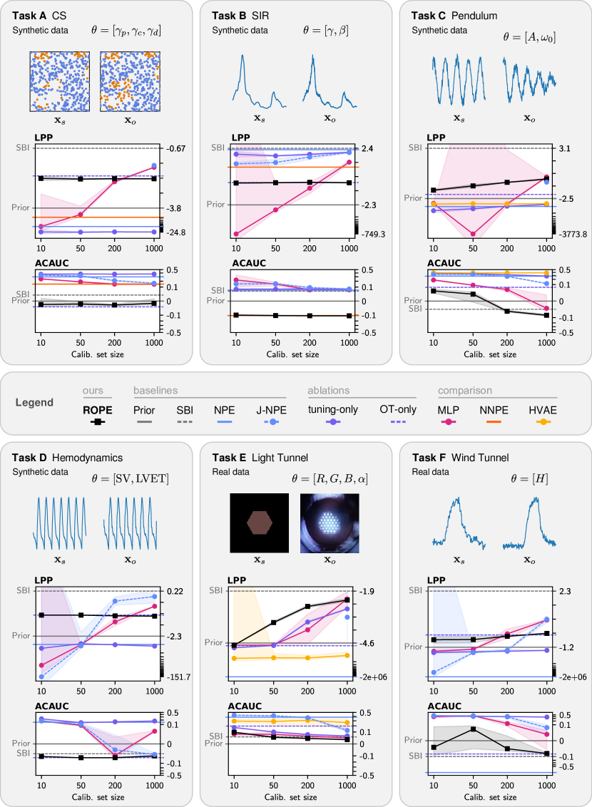
Figure 2: Results for our method (ROPE) and the competing baselines on six benchmark tasks. For each task, we show an example of the real observations ($\mathbf{x}_{o}$) and the observations produced by the misspecified simulator ($\mathbf{x}_{s}$). We show each method’s LPP and ACAUC metrics, as computed on a labeled test set of size 2000. We report the average metrics and $\pm 1$ std. deviation over three random draws of the test set and additional sources of randomness. In some instances, e.g., tasks A and E, the likelihood of J-NPE can be $-\infty$ and is not plotted. For readability of the LPP metric, we use a linear scale between the SBI and the Prior and a logarithmic scale for values below that.

Our experiments aim to (1) empirically validate the discussion in Section 3.2, and (2) illustrate settings in which our algorithm enables uncertainty quantification under model misspecification and small calibration datasets. The experiments comprise two existing benchmarks from the SBI literature, two synthetic benchmarks, and two new benchmarks from real physical systems for which both labeled data and simulators are available. To the best of our knowledge, the latter constitute the first real-world benchmarks for SBI under misspecified models. Altogether, the benchmarks represent various types of misspecification and parameter and observation space. We briefly describe each task and provide examples of real vs. simulated observations in Figure 2. Further details about the complete setup can be found in Appendix D.

Task A (synthetic): CS.

We reproduce the cancer and stromal cell development benchmark from Ward et al., (2022). The simulator emulates the development of cancer and stromal cells in a 2D environment as a function of three Poisson rate parameters $(\lambda_{c},\lambda_{p},\lambda_{d})$. The observations are vectors composed of the number of cancer and stromal cells and the mean and maximum distance between stromal cells and their nearest cancer cell. Synthetic misspecification is introduced by removing cancer cells that are too close to their generating parent.

Task B (synthetic): SIR.

We also use the stochastic epidemic model from Ward et al., (2022), which describes epidemic dynamics through the infection rate $\beta$ and recovery rate $\gamma$. Each observation is a vector composed of the mean, median, and maximum number of infections, the day of occurrence of the maximum number of infections, the day at which half the total number of infections was reached, and the mean auto-correlation (lag 1) of the infections. Misspecification is a delay in weekend infection counts, of which $5\%$ are added to the count of the following Monday.

Task C (synthetic): Pendulum.

The damped pendulum is a common benchmark to assess hybrid learning algorithms (Wehenkel et al.,, 2022), which jointly exploit domain knowledge and real-world data. The simulator generates the horizontal position of a friction-less pendulum given its fundamental frequency $\omega_{0}\in\mathbb{R}^{+}$ and amplitude $A\in\mathbb{R}^{+}$. Randomness enters the simulator through a random phase shift and white measurement noise. As misspecified “real-world” data, we simulate observations from a damped pendulum that takes friction into account.

Task D (synthetic): Hemodynamics.

Following Wehenkel et al., (2023), we define the task of inferring the stroke volume (SV) and the left ventricular ejection time (LVET) from normalized arterial pressure waveforms. The simulator is a PDE solver (Melis,, 2017) that produces an $8$-second time-series $\mathbf{x}_{s}$ sampled at $125$Hz. As synthetic misspecification, the simulator assumes all arteries have constant length, whereas this parameter varies in the “real-world” data.

Task E (real): Light Tunnel.

We employ one of the light tunnel datasets from Gamella et al., (2024). The tunnel is an elongated chamber with a controllable light source at one end, two linear polarizers mounted on rotating frames, and a camera. Our task consists of predicting the color setting of the light source ($(R,G,B)\in[0,255]^{3}$) and the dimming effect of the polarizers $\alpha\in[0,1]$ from the captured images. The simulator takes the parameters $\theta:=[R,G,B,\alpha]$ and produces an image consisting of a hexagon roughly the size of the light source, with a color equal to $[\alpha R,\alpha G,\alpha B]$.

Task F (real): Wind Tunnel.

We employ one of the wind tunnel datasets from Gamella et al., (2024). The tunnel is a chamber with two controllable fans that push air through it, and barometers that measure air pressure at different locations. A hatch controls the area of an additional opening to the outside. The dataset is a collection of pressure curves that result from applying a short impulse to the intake fan power and measuring the change in air pressure inside the tunnel. Our inference task consists of predicting the hatch position, $\theta:=H\in[0,45]$ given a pressure curve. As a simulator model, we adapt the physical model given in Gamella et al., (2024, Model C3, Appendix D).

Metrics

We consider two different metrics to assess whether ROPE provides reliable and useful uncertainty quantification. First, given a labeled test set $\{(\theta^{i},\mathbf{x}^{i}_{o})\}_{i=1}^{N}$, we compute the log-posterior probability (LPP) as

$$\text{LPP}:=\frac{1}{N}\sum_{i=1}^{N}\log\tilde{p}(\theta^{i}\mid\mathbf{x}_{o}^{i})\approx\mathbb{E}_{\begin{subarray}{c}p(\theta)\\ p(\mathbf{x}_{o}\mid\theta)\end{subarray}}\left[\log\tilde{p}(\mathbf{x}_{o}\mid\theta)\right].$$ (8)

The LPP is an empirical estimation of the expected cross entropy between the true and estimated posterior; thus, for an infinite test set, it is only maximized by the true posterior. LPP characterizes the entropy reduction on the estimation of $\theta$ achieved by a posterior estimator $\tilde{p}$ when given one observation, on average, over the test set. Second, the average coverage AUC (ACAUC) indicates the average calibration of $K$ 1D credible intervals extracted from the estimated posteriors, i.e.,

$$\text{ACAUC}:=\frac{1}{KN}\sum_{j=1}^{K}\sum_{i=1}^{N}\int_{0}^{1}\alpha-\mathbf{1}[\theta^{i}_{j}\in\Theta_{\tilde{p}(\theta_{j}\mid\mathbf{x}_{o}^{i})}(\alpha)]\text{d}\alpha,$$ (9)

where $\Theta_{\tilde{p}(\theta_{j}\mid\mathbf{x}_{o}^{i})}(\alpha)$ denotes the credible interval for the $\text{j}^{\text{th}}$ dimension of the parameter $\theta$ at level $\alpha$. Its value is positive (negative) if, on average over different credible levels, parameter dimensionality, and observations, the corresponding credible intervals are overconfident (underconfident). The ACAUC of a perfectly specified prior distribution is zero. The integral can be efficiently approximated, as described in Appendix F. For all experiments, we compute the LPP and ACAUC on labeled test set containing $2000$ pairs $(\theta,\mathbf{x}_{o})$.

Baselines

As a sanity check, we compare the performance of ROPE against four reference baselines: the prior $p(\theta)$, which amounts to the lower bound on the LPP for any calibrated posterior estimator; the SBI posterior on the simulated examples which, under the independence assumption $\mathbf{x}_{o}\perp\theta\mid\mathbf{x}_{s}$, is an upper bound on the LPP for ROPE; (NPE) a posterior estimator fitted to the simulated data and applied to the real data; and (J-NPE) a posterior estimator trained jointly on the pooled simulated and real observations. The latter two baselines represent some first approaches that a practitioner may consider. Additionally, we compare the performance of ROPE to MLP, which trains a neural network that predicts the mean and log-variance of a Gaussian posterior distribution by maximizing the calibration set log-likelihood. For the CS and SIR benchmarks, we additionally run Noisy NPE (NNPE, Ward et al.,, 2022), which improves the robustness of NPE by introducing a Spike and Slab error model on simulated data statistics. We do not run NNPE on tasks C-F, as this would be unfair for NNPE whose noise model is designed for low-dimensional statistics, as opposed to the temporal and spatial data considered in tasks C-F. Extending NNPE to such settings is out of the scope of our experiments. We also run the hybrid learning method HVAE (Takeishi and Kalousis,, 2021), which constitutes a strong baseline when the simulator can be made deterministic (tasks C and E) but is not directly applicable when the simulator is not differentiable. More details about each method and the experimental setup can be found in Appendix D.

4.1 Results

ROPE achieves robust posterior estimation for all tasks.

In Figure 2, we compare the performance of ROPE (with $\gamma=0.5$) against baselines for the $6$ tasks we consider. For all tasks, even with minimal calibration budgets, ROPE is the only method that consistently returns well-calibrated, or sometimes slightly under-confident, posterior estimation while significantly reducing uncertainty compared to the prior distribution. As the size of the calibration set increases, we see the adaptability of J-NPE and MLP as their performance improves and aligns with or outperforms ROPE. This adaptability is an expected behavior in IID settings, where real-world data eventually allows finding the minimizer of empirical risk among a class of predictors. However, on task E, where posteriors are complex conditional distributions—whose entropy increases with darker images and contain non-trivial dependencies between parameters—ROPE remains the best approach, even with a calibration set containing more than $1000$ examples. As an outlier, we observe that NPE trained on simulated data achieves the best results for the SIR benchmark (Task B), indicating that the misspecification of this benchmark is not a challenging test case for existing SBI methods. Finally, as interpreting a numerical gap in LPP metrics can be difficult, we complement these numerical results with visual corner plots for the two real-world experiments in Figure 3 and for all tasks in subsection E.1.

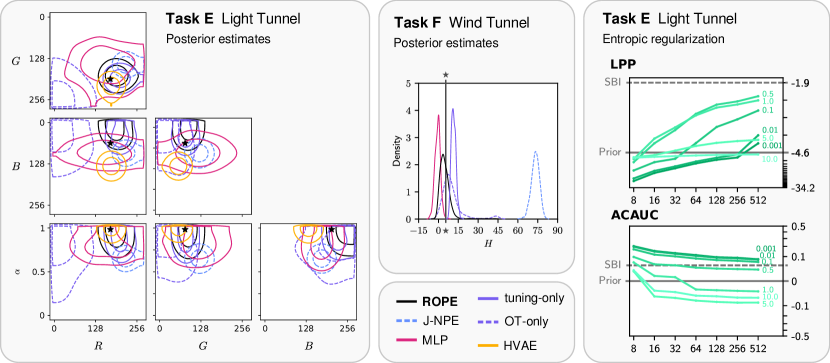
Figure 3: (left) Credible intervals of the posterior estimates at levels $65\%$ and $90\%$, for a single test sample from the light-tunnel task. The black stars denote the true value of the parameter. (center) Posterior estimates for a single test sample from the wind-tunnel task, where the true parameter is denoted by a vertical black line. (right) Effect of $\gamma$ on the LPP and ACAUC scores of ROPE on the light-tunnel task for different sizes of the calibration set. The value of $\gamma$ is shown by each curve. For reference, we plot the metrics achieved by the SBI posterior and prior distribution on simulated data.

Ablation study.

Our algorithm combines two steps with distinct roles: (1) a fine-tuning step, which improves the generalization domain of the NSE, and (2) an OT step, aiming to model the misspecification as a stochastic mapping between simulations and observations. To better understand their respective contribution to the performance of ROPE, we look at two ablated versions of our algorithm: tuning-only which appends the fine-tuned NSE to the NF trained on simulated data $p_{\phi^{\star}}$ and directly applies it to the real observations without an OT step; and OT-only, which directly performs OT with L2-norm in the original NSE space $c(\mathbf{x}_{o},\mathbf{x}_{s})=\lvert\mathbf{h}_{\omega^{\star}}(\mathbf{x}_{o})-\mathbf{h}_{\omega^{\star}}(\mathbf{x}_{s})\rvert_{2}$. In Figure 2, we observe that tuning-only’s result are poor except for Task B, for which misspecification is negligible. In contrast, for tasks A, D, and F, OT-only exhibits performance on par with ROPE. Nevertheless, ROPE can significantly outperform OT-only, such as in tasks C and E where the misspecification is significant. We conclude that the OT step is crucial and fine-tuning is sometimes necessary—we recommend that practitioners first evaluate OT-only’s performance and optimize the value of $\gamma$ before using a subset of the real-world data for fine-tuning.

Effect of entropic regularization.

In Figure 3, we study the effect of entropic regularization by varying the regularization parameter $\gamma$. For all values of $\gamma$, excluding $\gamma\geq 5$, we observe that both LPP and calibration consistently improve with the calibration set size. For large values of $\gamma$, the entropic regularization dominates and pushes toward a uniform mapping, resulting in posteriors that approximate the prior distribution, as highlighted in subsection 3.2. In these cases, the LPP barely changes with the calibration set size. These empirical results are consistent with the theoretical discussion in subsection 3.2. Furthermore, it is notable that the value of $\gamma$ does not excessively influence ROPE’s performance. As a recommendation for practitioners, our empirical evaluation suggests that values between $0.1$ and $1$ provide well-calibrated and precise credible intervals.

5 Discussion

While our experiments have demonstrated that ROPE enables reliable uncertainty quantification from misspecified simulator, our method and setup has certain shortcomings that we now discuss.

Prior misspecification.

While the importance of correct prior specification vanishes as the number of observations or sharpness of the likelihood function increases for well-specified likelihood models, the implications of violating it may severely damage ROPE’s performance because of the OT matching between simulated and real-world observations. As a possible solution, unbalanced OT (Séjourné et al.,, 2019; Fatras et al.,, 2021) relaxes the mass conservation constraint and could be an elegant solution to couple a subset of the simulations to the real-world data.

Curse of dimensionality.

The dimensionality of $\theta$ may impact two critical parts of ROPE. First, with each additional parameter $\theta[K+1]$, the NSE must encode up to $K$ dependence between $\theta[K+1]$ and other dimensions $\theta[1:K]$ given $\mathbf{x}_{o}$. While generating more simulations can address the curse of dimensionality in the simulation space, fine-tuning on a small calibration may not suffice anymore to cope with misspecification. Second, the dimensionality of the manifold on which the simulated and real-world observations are projected with the NSE grows and finding a meaningful matching between the two populations may require larger sample sizes. A potential solution is to focus marginal or 2D posterior distributions and ignore higher-dimensional dependencies in $p(\theta\mid\mathbf{x}_{o})$. Nevertheless, extending ROPE to such settings certainly opens new questions, e.g., on the development of better fine-tuning strategies that can leverage partial calibration sets where labels can be incomplete.

Other extensions.

Similarly to incomplete labels, certain applications have only access to noisy labels measured with a well-modeled, but noisy, measurement process. Further developing the fine-tuning stage to exploit such noisy labels would be necessary to make an approach similar to ROPE applicable. As another direction, leveraging inductive bias embedded into the neural network architecture of neural OT and the ability to better cope with large test set appears as a promising direction to amortize the mapping between simulation and real-world data. We believe following ROPE’s strategy of modeling misspecification in SBI as an OT coupling opens up several directions to cope with more specific problem setup.

Conclusion

In this paper, we have argued that model misspecification in simulation-based is a modeling issue that requires real-world labeled data to be solved. Under this premise, we have introduced ROPE, an algorithm that jointly exploits a small calibration set and optimal transport to extend neural posterior estimation for misspecified simulators. Our experiments on diverse benchmarks, demonstrate ROPE’s ability to estimate well-calibrated and informative posterior distributions for various simulators and real-world examples. As a conclusion, ROPE is a simple method that practitioners can use to predict calibrated posterior over the parameter of misspecified simulator on real-world data.

Broader Impact

This paper presents a framework and an algorithm to address model misspecification in simulation-based inference (SBI). SBI is predominantly applied in scientific fields where complex simulators of physical phenomena are available, such as astronomy, particle physics, or climate modeling. A priori, this circumscribes the application of our algorithm to highly specialized scientific domains in the natural sciences, precluding issues such as fairness or privacy. However, its application to the scientific domain is not exempt from societal or ethical implications, particularly when computer simulations may inform research or policy decisions. In this regard, we find some properties of the algorithm particularly promising, such as uncertainty quantification and the limitation of not drawing conclusions beyond the given expert model. However, much more work is needed to deeply understand the reliability of these properties and how they are affected by violations of the core assumptions, such as a well-specified prior. Such work should precede any sort of over-selling to practitioners about the benefits of the algorithm. Rather, we see our work as an academic contribution towards a more broad and successful application of SBI techniques; success in this endeavor, as for the establishment of any scientific tool, will require an iterative dialogue between the scientists who develop the methodology and those who use it.

Appendix A Robustness to distribution shifts

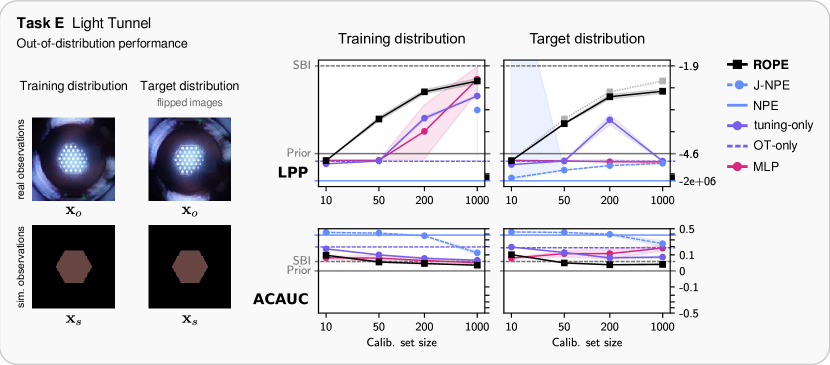
Figure 4: Out-of-distribution performance of ROPE and some baselines. We train ROPE and other baselines on the same light-tunnel data as in task E (training distribution), but apply it to test sets originating from a target distribution where the real-world images are flipped vertically. We compare the performance on test sets from both distributions, showing the LPP and ACAUC scores for each method. For comparison, in the right plot we show again the LPP curve (light gray, dotted) attained by ROPE under the training distribution. The performance of ROPE is barely affected as it cannot exploit any signal in the real images ($\mathbf{x}_{o}$) beyond what is encoded in the simulator, and the simulator output ($\mathbf{x}_{s}$) is invariant to the transformation we consider. Because NPE is not trained on real observations, its performance, although poor, also remains virtually unchanged. On the other hand, the performance of MLP and J-NPE drops in the target distribution, as these methods are not limited in what information they can exploit from the real observations on which they are trained, potentially learning shortcuts that are not present in the target distribution. This results demonstrate that if the simulator embeds the right invariances, our modeling assumption $\mathbf{x}_{o}\perp\theta\mid\mathbf{x}_{s}$ can be favorable to out-of-distribution generalization.

Appendix B Self-calibration Property

We say ROPE is self-calibrating because, by design, the posterior distribution marginalized over observations tends to the prior as the number of simulation increases, that is,

$$\int\tilde{p}(\theta\mid\mathbf{x}_{o})p(\mathbf{x}_{o})=p(\theta).$$ (10)

This property is also called marginal calibration as it is a necessary condition for a posterior estimation method to be calibrated. Considering NPE, $\tilde{p}(\theta\mid\mathbf{x}_{s})$, is marginally calibrated and observations $\mathbf{x}_{o}$ are generated from the assumed prior, that is sampled from an unknown distribution $p(\mathbf{x}_{o})=\int p(\mathbf{x}_{o}\mid\theta)p(\theta)$, we can show ROPE is marginally calibrated. Indeed, considering the Monte-Carlo approximation of the marginalized posterior distribution over the test set $\mathcal{D}_{o}:=\{\mathbf{x}_{o}\}_{i=1}^{N_{o}}$, we have,

$$\int\tilde{p}(\theta\mid\mathbf{x}_{o})p(\mathbf{x}_{o}) \approx\frac{1}{N_{o}}\sum_{i=1}^{N_{o}}\tilde{p}(\theta\mid\mathbf{x}_{o})$$ (11)

$$=\frac{1}{N_{o}}\sum_{i=1}^{N_{o}}\sum_{j=1}^{N_{s}}N_{o}P^{\star}_{ij}\tilde{p}(\theta\mid\mathbf{x}_{s}^{j})$$ (12)

$$=\sum_{j=1}^{N_{s}}\left[\sum_{i=1}^{N_{o}}P^{\star}_{ij}\right]\tilde{p}(\theta\mid\mathbf{x}_{s}^{j})$$ (13)

$$=\frac{1}{N_{s}}\sum_{j=1}^{N_{s}}\tilde{p}(\theta\mid\mathbf{x}_{s}^{j})$$ (14)

$$\approx p(\theta),$$ (15)

where we use the definition of the transport matrix to get $\sum_{i=1}^{N_{o}}P^{\star}_{ij}=\frac{1}{N_{s}}$. The last approximation tends to be exact as the number of simulations increases, if the NPE is marginally calibrated.

Appendix C ROPE Algorithm

Algorithm 1 Posterior Inference using Robust Neural Posterior Estimation (ROPE)

  Input: Simulator $S(\theta,\varepsilon)$, prior distribution $p(\theta)$, calibration set $\mathcal{C}=\{(\mathbf{x}_{o}^{i},\theta^{i})\}_{i=1}^{N_{c}}$, test set $\mathcal{D}=\{\mathbf{x}_{o}^{i}\}_{i=1}^{N_{o}}$

  Output: $\tilde{p}(\theta\mid\mathbf{x}_{o})\forall\mathbf{x}^{i}_{o}\in\mathcal{D}$

  Step 1: Neural Posterior Estimation (NPE)

  Train neural network $\mathbf{h}_{\omega}$ and conditional normalizing flow $p(\theta\mid\cdot)$ using NPE:

$$\tilde{p},\omega^{\star}= \arg\max_{p,\omega}\mathbb{E}_{\begin{subarray}{c}\theta\sim\pi(\theta)\\ \varepsilon\sim\mathcal{U}[0,1]\end{subarray}}\left[\log p(\theta\mid\mathbf{h}_{\omega}(S(\theta,\epsilon)))\right]$$

  Step 2: Fine-tune sufficient statistics $\mathbf{h}_{\omega^{\star}}$ on the Calibration Set

  $\mathbf{g}_{\psi}:=\text{COPY}(\mathbf{h}_{\omega^{\star}})$

  $\mathcal{C}_{train},\mathcal{C}_{val}=\text{RandomSplit}(\mathcal{C},\frac{1}{5})$

  $\text{best}_{val}=\infty$

  for $N_{\text{iter}}$ do

     $\psi\leftarrow\psi-\alpha\nabla_{\psi}\left[\sum_{(\theta,\mathbf{x}_{o})\in\mathcal{C}_{train}}\lvert\mathbf{g}_{\psi}(\mathbf{x}_{o})-\mathbb{E}_{\varepsilon}[\mathbf{h}_{\omega^{\star}}(S(\theta,\varepsilon))]\rvert_{2}\right]$

     $\text{cur}_{val}=\sum_{(\theta,\mathbf{x}_{o})\in\mathcal{C}_{val}}\lvert\mathbf{g}_{\psi}(\mathbf{x}_{o})-\mathbb{E}_{\varepsilon}[\mathbf{h}_{\omega^{\star}}(S(\theta,\varepsilon))]\rvert_{2}$

     if $\text{cur}_{val}<\text{best}_{val}$ then

        $\text{best}_{val}=\text{cur}_{val}$

        $\psi^{\star}=\psi$

     end if

  end for

  Step 3: Generate Simulations for Test Set ($N_{s}=N_{o}$)

  $\mathcal{S}=\{\mathbf{x}_{s}^{j}\}_{j=1}^{N_{s}},$where $\mathbf{x}_{s}^{j}\sim S(\theta^{j},\varepsilon)\quad\theta^{j}\sim\pi(\theta)\quad\varepsilon\sim\mathcal{U}[0,1]$

  Step 4: Entropic-regularized OT

$$P^{\star}= \arg\min_{P\in\mathcal{B}}\sum_{ij}^{N_{o}\times N_{s}}P_{ij}\left(\lvert f_{\omega^{\star}}(\mathbf{x}_{s}^{j})-g_{\psi^{\star}}(\mathbf{x}_{o}^{i})\rvert+\gamma\log P_{ij}\right)$$

  Step 5: Compute Posterior Distributions

$$p(\theta|\mathbf{x}_{o}^{i}):=\sum_{j=1}^{N_{s}}P^{\star}_{ij}\tilde{p}\left(\theta\mid\mathbf{h}_{\omega^{\star}}(\mathbf{x}_{s}^{j})\right)$$

  Return $\tilde{p}(\theta|\mathbf{x}_{o}^{i})\quad\forall\mathbf{x}_{o}^{i}\in\mathcal{D}$

Appendix D Experimental Setup

In this section, we provide more details on our experiments. For completeness, we provide details on the neural architectures and training hyperparameters. However, we encourage the reader interested in reproducing our experiments to examine our code directly (a link to the code will be made available in the public version of the paper).

For all methods training on calibration set we keep always keep $20\%$ of the calibration to monitor validation performance and we select the best model based on this metric.

For the MLP we use the same architecture as the NSE for all our experiments and optimize its parameters on the calibration set with Adam and a learning rate equal to $0.0003$, we select the best model based on the LPP attributed to the validation subset of the calibration set.

D.1 Task A: CS & Task B: SIR

We refer the reader to Ward et al., (2022) for more details about the simulator and prior distribution. We use the exact same setting as theirs.

Neural architecture & Training Hyperparameters

For all methods we use the same backbone MLP as the NSE with ReLU activations and layers composed of $[4K,16K,16K,12K,3K]$ neurons, where $K$ is the dimensionality of $\theta$. The NF is a 1-step UMNN-MAF (Wehenkel and Louppe,, 2019) with $[100,100,100]$ neurons for both the autoregressive conditioner and normalizer. For NNPE, we train the UMNN-MAF on simulations poluted by Spike and Slab errors. We train models with Adam and a learning rate equal to $0.0005$ and all other parameters set to default. We optimize the SBI model for $10^{6}$ gradient steps and select the best model on random validation sets containing $10^{5}$ simulations.

D.2 Task C: Pendulum

Description

The first task is inspired from the damped pendulum benchmark commonly used to assess hybrid learning algorithms. Given a $2$D physical parameter $\theta:=[\omega_{0},A]$, where $\omega_{0}\in\mathbb{R}^{+}$ denotes the fundamental frequency and $A\in\mathbb{R}^{+}$ the amplitude of a friction-less pendulum, the simulator generates the horizontal position of the pendulum at $200$ discrete times during uniformly sampled in a $10$ seconds interval as

$$\mathbf{x}_{s}:=[\theta(t=0),\dots,\theta(t=10s)]\in\mathbb{R}^{200}$$

$$\text{ where }\theta(t)=A\cos(\omega_{0}t+\varphi)\quad\varphi\sim\mathbb{U}(-\pi,\pi).$$ (16)

The relationship between the parameters and the simulation is thus stochastic as $\varphi$ accounts for an unknown phase shift when the measurements start. We generate real-world observations synthetically by replacing $\theta(t)$ from (16) by

$$\tilde{\theta}(t)=e^{\alpha t}A\cos(\omega_{0}t+\varphi)\quad\varphi\sim\mathbb{U}[-\pi,\pi]\quad\alpha\sim\mathbb{U}[0,1],$$

where $\alpha$ represents the effect of friction. We also add Gaussian noise on both simulated and real-world data to represent the inaccuracy of a sensor measuring the pendulum’s position. The prior distribution is a product of uniform distribution, $p(\theta:=[\omega_{0},A])=\mathcal{U}[0,3]\times\mathcal{U}[0.5,10]$.

Neural architecture & Training Hyperparameters

Neural Posterior Estimator.

The NSE is a 1D convolutional neural network, with the architecture described in Algorithm 2.

Algorithm 2 Convolutional Neural Network for Tasks A and D.

1:  $\text{Conv1d}(1,16,3,1,\text{dilation}=2,\text{padding}=1)$

2:  $\text{ReLU}()$

3:  $\text{Conv1d}(16,64,3,2,\text{dilation}=2,\text{padding}=1)$

4:  $\text{ReLU}()$

5:  $\text{AvgPool1d}(3,1)$

6:  $\text{Conv1d}(64,128,3,1,\text{dilation}=2,\text{padding}=1)$

7:  $\text{ReLU}()$

8:  $\text{Conv1d}(128,128,3,2,\text{dilation}=2,\text{padding}=1)$

9:  $\text{ReLU}()$

10:  $\text{AvgPool1d}(3,1)$

11:  $\text{Conv1d}(128,128,3,1,\text{dilation}=2,\text{padding}=1)$

12:  $\text{ReLU}()$

13:  $\text{Conv1d}(128,128,3,2,\text{dilation}=2,\text{padding}=1)$

14:  $\text{ReLU}()$

15:  $\text{AvgPool1d}(3,1)$

16:  $\text{Conv1d}(128,128,3,1,\text{dilation}=2,\text{padding}=1)$

17:  $\text{ReLU}()$

18:  $\text{Flatten}()$

19:  $\text{Linear}(2048,512)$

20:  $\text{ReLU}()$

21:  $\text{Linear}(512,128)$

22:  $\text{ReLU}()$

23:  $\text{Linear}(128,32)$

24:  $\text{ReLU}()$

25:  $\text{Linear}(32,10)$

The NCDE is a one-step discrete normalizing flow with an autoregressive conditioner and a UMNN (Wehenkel and Louppe,, 2019) as the normalizer. The autoregressive conditioner is a MADE with ReLU activation and $3$ layers of $100$ neurons that output a $10$ dimensional vector to the UMNN. The UMNN has an integrand net with $3$ layers of $100$ neurons with ReLU activations. For training the NPE, we use a batch size of $100$ and a learning factor equal to 1e-4. NPE is trained until convergence. Other parameters are set to default values and should marginally impact the NPE obtained.

ROPE NSE.

We have selected the best NPE based on the validation set with $10000$ examples generated with the simulator. The NPE is fixed to one best-of-all model. We fine-tune the NCDE with a learning rate equal to 1e-5 for $5000$ gradient steps on $80\%$ the full calibration set. We use a 1-sample Monte Carlo estimate of the expectation in (7).

J-NPE

To train J-NPE, we simply randomly use a batch composed of $50\%$ of simulated pairs $(\theta,\mathbf{x}_{s})$ and of $50\%$ $(\theta,\mathbf{x}_{o})$ from the calibration set. We use the same architecture and hyper-parameters as the SBI NPE. The best model is selected based on the best training set performance. We do $50$ epochs with $50000$ simulated examples for each epoch. The batch size is $100$.

HVAE

For the HVAE, we re-use the NPE model as the physics encoder and replace the decoder with a deterministic version of the simulator, thus removing the Gaussian noise on a random phase shift. In addition, we follow the approach of Takeishi and Kalousis, (2021) and have 1) a real-world encoder that maps $\mathbf{x}_{o}$ to $\mathbf{z}_{a}$, 2) a reality-to-physics encoder, and 3) a physics-to-reality decoder. The real-world encoder has the same architecture as the NSE of the NPE and outputs the mean and log-variance of a $5$D latent vector $\mathbf{z}_{a}$. The reality-to-physics and physics-to-reality also have the same architectures and are two conditional 1D U-Net with neural network architecture described in Algorithm 3.

Algorithm 3 UNet1D Architecture

1:  $\text{Unet1D}:$

2:   $\text{Encoder1D}:$

3:    $\text{Block}(\text{in\_channels}=1,\text{out\_channels}=64)$

4:    $\text{Block}(\text{in\_channels}=64,\text{out\_channels}=128)$

5:    $\text{Block}(\text{in\_channels}=128,\text{out\_channels}=256)$

6:    $\text{Block}(\text{in\_channels}=256,\text{out\_channels}=512)$

7:    $\text{Block}(\text{in\_channels}=512,\text{out\_channels}=1024)$

8:    $\text{MaxPool1d}(2)$

9:   $\text{Decoder1D}:$

10:    $\text{ConvTranspose1d}(1024+5,512,2,\text{stride}=2)$

11:    $\text{Block}(\text{in\_channels}=1024,\text{out\_channels}=512)$

12:    $\text{ConvTranspose1d}(512,256,2,\text{stride}=2)$

13:    $\text{Block}(\text{in\_channels}=512,\text{out\_channels}=256)$

14:    $\text{ConvTranspose1d}(256,128,2,\text{stride}=2)$

15:    $\text{Block}(\text{in\_channels}=256,\text{out\_channels}=128)$

16:    $\text{ConvTranspose1d}(128,64,2,\text{stride}=2)$

17:    $\text{Block}(\text{in\_channels}=128,\text{out\_channels}=64)$

18:    $\text{ConvTranspose1d}(64,1,2,\text{stride}=2)$

19:    $\text{Block}(\text{in\_channels}=64,\text{out\_channels}=1)$

20:    $\text{Conv1d}(64,1,1)$

Algorithm 4 Block1D(in_channels, out_channels)

1:  Conv1d(in_channels, out_channels, kernel_size=3, padding=1)

2:  ReLU()

3:  Conv1d(out_channels, out_channels, kernel_size=3, padding=1)

4:  ReLU()

Algorithm 5 $2$D Convolutional Neural Network

1:  Conv2d(3, 64, 3, 2, dilation=1), ReLU()

2:  Conv2d(64, 128, 3, 2, dilation=1), ReLU()

3:  MaxPool2d(3)

4:  Conv2d(128, 128, 3, 2, dilation=1), ReLU()

5:  Conv2d(128, 64, 1, 1, dilation=1), ReLU()

6:  Conv2d(64, 3, 1, 1, dilation=1), ReLU()

7:  Flatten()

8:  Linear(27, 100), ReLU()

9:  Linear(100, 20)

To train the HVAE, we freeze the parameters of the NPE and optimizes the ELBO as well as a calibration loss that evaluates the likelihood assigned to the true physical parameters. All distributions are parameterized by Gaussian with mean and log-variance predicted by the neural networks. We do not use any additional losses as we expect constraining NPE and using the calibration set should already provide the necessary support to use the physics in a meaningful way. The HVAE is trained on the $2000$ test examples as it is the only real-world data, calibration set aside, that we have access to. We use a batch size equal to $100$ and a learning rate equal to 1e-3. We believe obtaining a better HVAE is possible. However, we emphasize the complexity of setting up a good HVAE for the only purpose of statistical inference over parameters.

Datasets

For this task, we can generate samples $(\theta,\mathbf{x}_{s})$ on the fly to train the NPE. The calibration and test sets are also generated randomly by sampling from the prior distribution and using the damped pendulum simulator.

D.3 Task D: Hemodynamics

Description

Inspired by Wehenkel et al., (2023), we define the task of inferring important cardiovascular parameters from normalized arterial pressure waveforms measured at the radial artery. The simulator uses many physiological parameters that modulates the heart function, physical properties of the $116$ main arterial segments, and behavior of the vascular beds. Our inference concerns two parameters of the heart function, $\theta:=[\text{SV},\text{LVET}]$, the stroke volume (SV) is the amount pumped out from the left ventricle over the heart beat modeled, and the left ventricular ejection time (LVET) is the time interval between opening and closure of the aortic valve. Other parameters, such as the heart rate or arteries’ stiffness, are considered as nuisance effects and are randomly sampled from a realistic population distribution. An additional source of randomness is added by modeling measurement errors with a white Gaussian noise and randomizing the starting recording time with respect to the cardiac cycle. The simulator produces $8$-second timeseries $\mathbf{x}_{t}\in\mathbb{R}^{1000}$ sampled at $125Hz$. As synthetic misspecification, the simulator assumes all arteries have the same length over the population considered, whereas "real-world" data are artificially generated by also varying the length of arteries and account for the effect of human’s height. The simulator is based on the openBF PDE solver (Melis,, 2017) specialized for hemodynamics, which is not differentiable and takes approximately one minute to simulate one sample on a standard CPU. This synthetic tasks represent a common scenario in which a simulator, although faithful to the effect of certain parameters, misses additional degrees of freedom that exists for the real-world data.

Neural architecture & Training Hyperparameters

Algorithm 6 CNN Architecture for Task C.

1:  Conv1d(1, 16, 3, 1, dilation=2, padding=1), ReLU()

2:  Conv1d(16, 64, 3, 2, dilation=2, padding=1), ReLU()

3:  AvgPool1d(4, 2)

4:  Conv1d(64, 128, 3, 1, dilation=2, padding=1), ReLU()

5:  Conv1d(128, 128, 3, 2, dilation=2, padding=1), ReLU()

6:  AvgPool1d(4, 2)

7:  Conv1d(128, 128, 3, 1, dilation=2, padding=1), ReLU()

8:  Conv1d(128, 128, 3, 2, dilation=2, padding=1), ReLU()

9:  AvgPool1d(4, 1)

10:  Conv1d(128, 128, 3, 1, dilation=2, padding=1), ReLU()

11:  Flatten()

12:  Linear(1024, 512), ReLU()

13:  Linear(512, 128), ReLU()

14:  Linear(128, 32), ReLU()

15:  Linear(32, 5)

Neural Posterior Estimator.

The NSE is the 1D convolutional neural network described in Algorithm 6. The NCDE is a $5$-step discrete normalizing flow with an autoregressive conditioner and affine normalizers. Each of the $5$ autoregressive conditioners is a MADE with ReLU activations and $4$ layers of $300$ neurons that output $4$ dimensional vectors used to parameterize the affine transformations. For training the NPE, we use a batch size of $100$ and a learning factor equal to 5e-4. NPE is trained until convergence. Other parameters are set to default values and should marginally impact the NPE obtained.

ROPE NSE.

We have selected the best NPE based on the validation set with $2000$ examples generated with the simulator. The NPE is fixed to one best-of-all model. We fine-tune the NCDE with a learning rate equal to 1e-5 for $2000$ gradient steps on $80\%$ of calibration set. We use a 1-sample Monte Carlo estimate of the expectation in (7).

J-NPE

To train J-NPE, we simply randomly use a batch composed of $50\%$ of simulated pairs $(\theta,\mathbf{x}_{s})$ and of $50\%$ $(\theta,\mathbf{x}_{o})$ from the calibration set. We use the same architecture and hyper-parameters as the SBI NPE. The best model is selected based on the best training set performance. We do $50$ epochs with $6000$ simulated examples for each epoch. The batch size is $100$.

HVAE

There is no HVAE for this experiment as the simulator is non-differentiable.

Datasets

For this task, we cannot generate samples $(\theta,\mathbf{x}_{s})$ on the fly to train the NPE. For the purpose of this experiment, we have generated $10000$ simulations and real-world observations. Our fine-tuning strategy approximates (7) by finding the simulations with the closest parameter value.

D.4 Task E: Light Tunnel

Description

We use one of the light-tunnel datasets from the causal chamber project (Gamella et al.,, 2024, causalchamber.org). In particular, we use the data from the ap_1.8_iso_500.0_ss_0.005 experiment in the lt_camera_v0 dataset. The light tunnel is an elongated chamber with a controllable light source at one end, two linear polarizers mounted on rotating frames, and a camera that takes images of the light source through the polarizers. We refer the reader to Gamella et al., (2024, Figure 2) for a complete schematic. Our task consists of predicting the color setting of the light source ($(R,G,B)\in[0,255]^{3}$) and the dimming effect of the linear polarizers $\alpha\in[0,1]$ from the captured images. As a misspecified simulator of the image-generating process, we adopt the simple model described in Gamella et al., (2024, Model F1, Appendix D). A Python implementation is available through the causalchamber package (models.model_f1); visit causalchamber.org for more details. As input, the simulator takes the parameters $\theta:=[R,G,B,\alpha]$ and produces an image consisting of a hexagon roughly the size of the light source, with an RGB color vector equal to $[\alpha R,\alpha G,\alpha B]$. The factor $\alpha:=\cos^{2}(\theta_{1}-\theta_{2})$, where $\theta_{1},\theta_{2}$ denote the angles of the two polarizers, corresponds to Malus’ law (e.g. , Collett,, 2005), which models the dimming effect of the polarizers as a function of their relative angle. Besides the obvious misspecification with respect to image realism (see Figure 2), the model ignores other important physical aspects, such as the spectral response of the camera sensor or the non-uniform effect of the polarizers on the different colors—more details can be found in Gamella et al., (2024, Appendix D.IV.2.2). The prior is uniform over colors and polarizer angles, which leads to a non-uniform prior over the dimming effect $\alpha$.

Neural architecture & Training Hyperparameters

Neural Posterior Estimator.

The NSE is the 2D convolutional neural network described by Algorithm 5.

The NCDE is also a one-step discrete normalizing flow with an autoregressive conditioner and a UMNN (Wehenkel and Louppe,, 2019) as the normalizer. The autoregressive conditioner is a MADE with ReLU activation and $3$ layers of $500$ neurons that outputs a $10$ dimensional vector to the UMNN. The UMNN has an integrand net with $4$ layers of $150$ neurons with ReLU activations. For training the NPE, we use a batch size of $100$ and a learning factor equal to 5e-4. NPE is trained until convergence. Other parameters are set to default values and should marginally impact the NPE obtained.

ROPE NSE.

We have selected the best NPE based on the validation set with $10000$ examples generated with the simulator. The NPE is fixed to one best-of-all model. We fine-tune the NCDE with a learning rate equal to 1e-4 for $2000$ gradient steps on on $80\%$ of the calibration set. We use a 1-sample Monte Carlo estimate of the expectation in (7).

J-NPE

To train J-NPE, we simply randomly use a batch composed of $50\%$ of simulated pairs $(\theta,\mathbf{x}_{s})$ and of $50\%$ $(\theta,\mathbf{x}_{o})$ from the calibration set. We use the same architecture and hyper-parameters as the SBI NPE. The best model is selected based on the best training set performance. We do $50$ epochs with $1000$ simulated examples for each epoch. Simulations are generated randomly for each batch by sampling the prior and simulating for the corresponding parameters. The batch size is $100$.

HVAE

For the HVAE, we re-use the NPE model as the physics encoder and use the simulator as is as it is differentiable without additional effort. In addition, we follow the approach of Takeishi and Kalousis, (2021) and have 1) a real-world encoder that maps $\mathbf{x}_{o}$ to $\mathbf{z}_{a}$, 2) a reality-to-physics encoder, and 3) a physics-to-reality decoder. The real-world encoder has the same architecture as the NSE of the NPE and outputs the mean and log-variance of a $5$D latent vector $\mathbf{z}_{a}$. The reality-to-physics and physics-to-reality also have the same architectures and are two conditional 2D U-Net with the architecture described by Algorithm 7.

Algorithm 7 2D UNet

1:  Encoder2D:

2:   Block2D(in_channels=3, out_channels=64)

3:   Block2D(in_channels=64, out_channels=128)

4:   Block2D(in_channels=128, out_channels=256)

5:   Block2D(in_channels=256, out_channels=512)

6:   Block2D(in_channels=512, out_channels=1024)

7:   MaxPool2d(2)

8:  Decoder2D:

9:   ConvTranspose2d(1024 + 5, 512, 2, stride=2)

10:   Block2D(in_channels=1024, out_channels=512)

11:   ConvTranspose2d(512, 256, 2, stride=2)

12:   Block2D(in_channels=512, out_channels=256)

13:   ConvTranspose2d(256, 128, 2, stride=2)

14:   Block2D(in_channels=256, out_channels=128)

15:   ConvTranspose2d(128, 64, 2, stride=2)

16:   Block2D(in_channels=128, out_channels=64)

17:   ConvTranspose2d(64, 1, 2, stride=2)

18:   Block2D(in_channels=64, out_channels=1)

19:   Conv2d(64, 1, 1)

Algorithm 8 Block2D(in_channels, out_channels)

1:  Conv2d(in_channels, out_channels, kernel_size=3, padding=1, bias=False)

2:  BatchNorm2d(num_features=out_channels)

3:  ReLU(inplace=True)

4:  Conv2d(out_channels, out_channels, kernel_size=3, padding=1, bias=False)

5:  BatchNorm2d(num_features=out_channels)

6:  ReLU(inplace=True)

To train the HVAE, we freeze the parameters of the NPE and optimizes the ELBO as well as a calibration loss that evaluates the likelihood assigned to the true physical parameters. All distributions are parameterized by Gaussian with mean and log-variance predicted by the neural networks. We do not use any additional losses as we expect constraining NPE and using the calibration set should already provide the necessary support to use the physics in a meaningful way. The HVAE is trained on the $2000$ test examples as it is the only real-world data, calibration set aside, that we have access to. We use a batch size equal to $100$ and a learning rate equal to 1e-3. We believe obtaining a better HVAE is possible. However, we emphasize the complexity of setting up a good HVAE for the only purpose of statistical inference over parameters.

Datasets

For this task, we can generate samples $(\theta,\mathbf{x}_{s})$ on the fly to train the NPE. However, the calibration and test sets are real-world data. We ensure there is not overlap between calibration and test set. The is no randomization and the test set is constant for all experiments, the calibration set are also fixed for a given calibration set size.

D.5 Task F: Wind Tunnel

Description

We use one of the wind-tunnel datasets from the causal chamber project (Gamella et al.,, 2024, causalchamber.org). In particular, we use the data from the load_out_0.5_osr_downwind_4 experiment in the wt_intake_impulse_v1 dataset. The tunnel is a chamber with two controllable fans that push air through it and barometers that measure air pressure at different locations. A hatch precisely controls the area of an additional opening to the outside (see Gamella et al.,, 2024, Figure 2). The data is a collection of pressure curves that result from applying a short impulse to the intake fan load and measuring the change in air pressure using one of the barometers inside the tunnel. Our inference task consists of predicting the hatch position, $\theta:=[H]\in[0,45]$ given a pressure curve (see Figure 2). As a simulator model, we combine the models A2 and C3 described in Gamella et al., (2024, Appendix D); we numerically solve the ODE in model A2, and add stochastic components to simulate the sensor noise and the unknown time point at which the impulse is applied. This results in the simulator being neither differentiable nor deterministic. A Python implementation of the complete simulator is available in the causalchamber package (models.simulator_a2_c3); visit causalchamber.org for more details. Misspecification arises from the many simplifying assumptions needed to model the complex dynamics of the airflow inside the tunnel—more details can be found in Gamella et al., (2024, Appendix D.IV.1.2).

Neural Posterior Estimator.

The NSE and NCDE have the same 1D convolutional neural network as for Task A. For training the NPE, we use a batch size of $100$ and a learning factor equal to 5e-4. NPE is trained until convergence. Other parameters are set to default values and should marginally impact the NPE obtained.

ROPE NSE.

We have selected the best NPE based on the validation set with $10000$ examples generated with the simulator. The NPE is fixed to one best-of-all model. We fine-tune the NCDE with a learning rate equal to 1e-4 for $20000$ gradient steps on on $80\%$ of the calibration set. We use a 1-sample Monte Carlo estimate of the expectation in (7).

J-NPE.

To train J-NPE, we simply randomly use a batch composed of $50\%$ of simulated pairs $(\theta,\mathbf{x}_{s})$ and of $50\%$ $(\theta,\mathbf{x}_{o})$ from the calibration set. We use the same architecture and hyper-parameters as the SBI NPE. The best model is selected based on the best training set performance. We do $50$ epochs with $10000$ simulated examples for each epoch. The batch size is $100$.

HVAE.

There is no HVAE for this experiment as the simulator is non-differentiable.

Datasets

For this task, although slightly slower than Task A and B, we can generate samples $(\theta,\mathbf{x}_{s})$ on the fly to train the NPE. However, the calibration and test sets are real-world data. We ensure no overlap between the two sets for all calibration set sizes. All sets are fixed for all experiments.

Appendix E Additional results

E.1 Corner plots

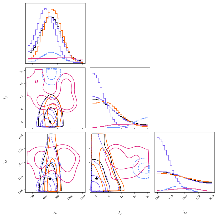
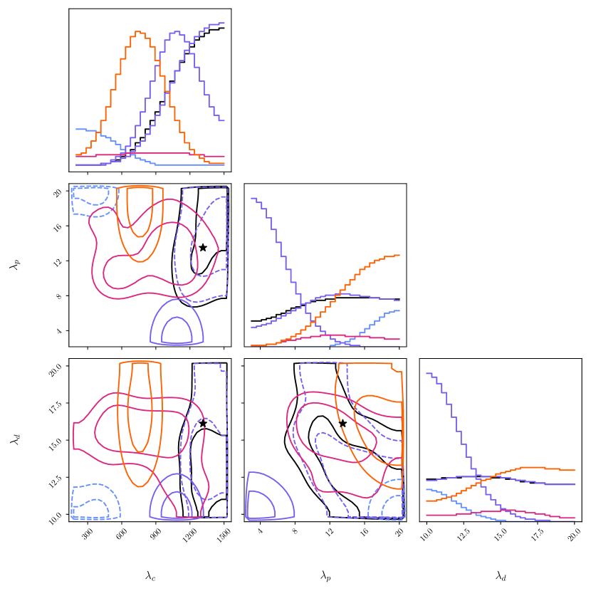
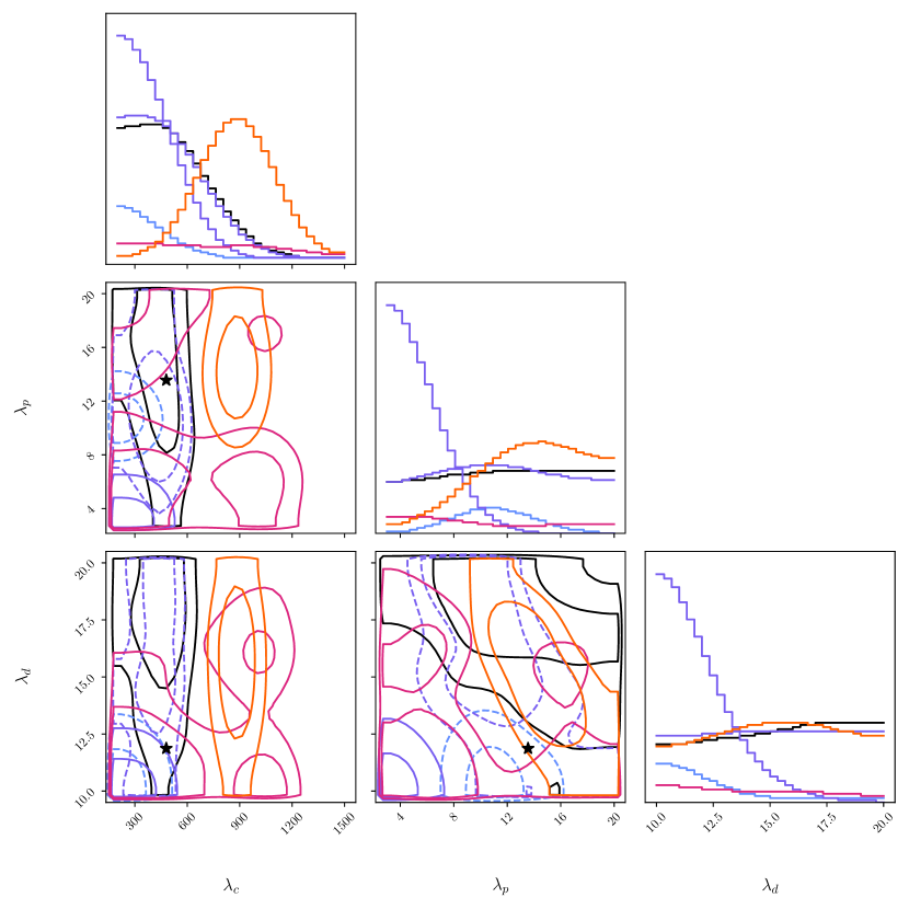
Figure 5: Three corner plots for task A with a calibration set with $50$ samples.

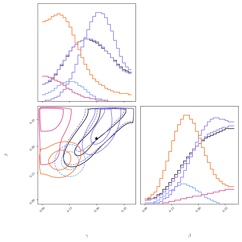
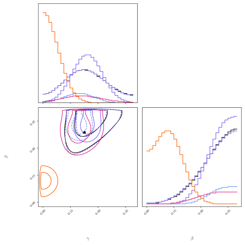
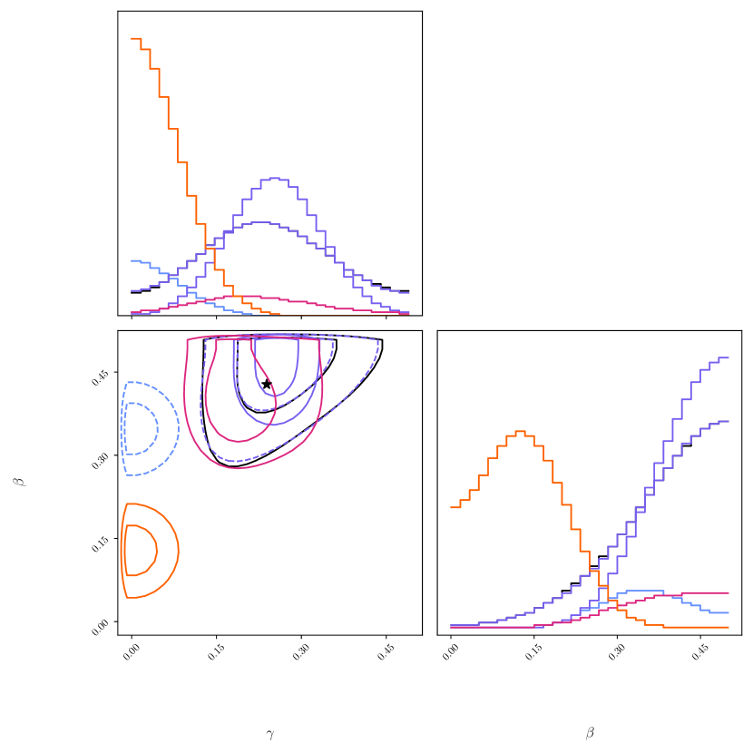
Figure 6: Three corner plots for task B with a calibration set with $50$ samples.

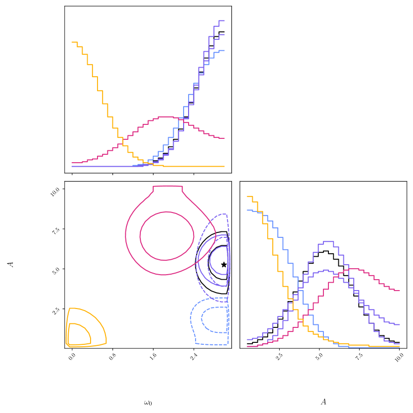
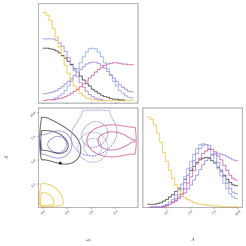
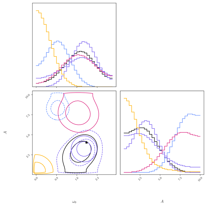
Figure 7: Three corner plots for task C with a calibration set with $50$ samples.

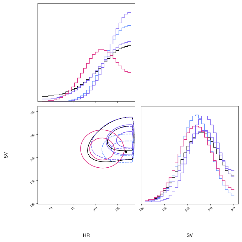
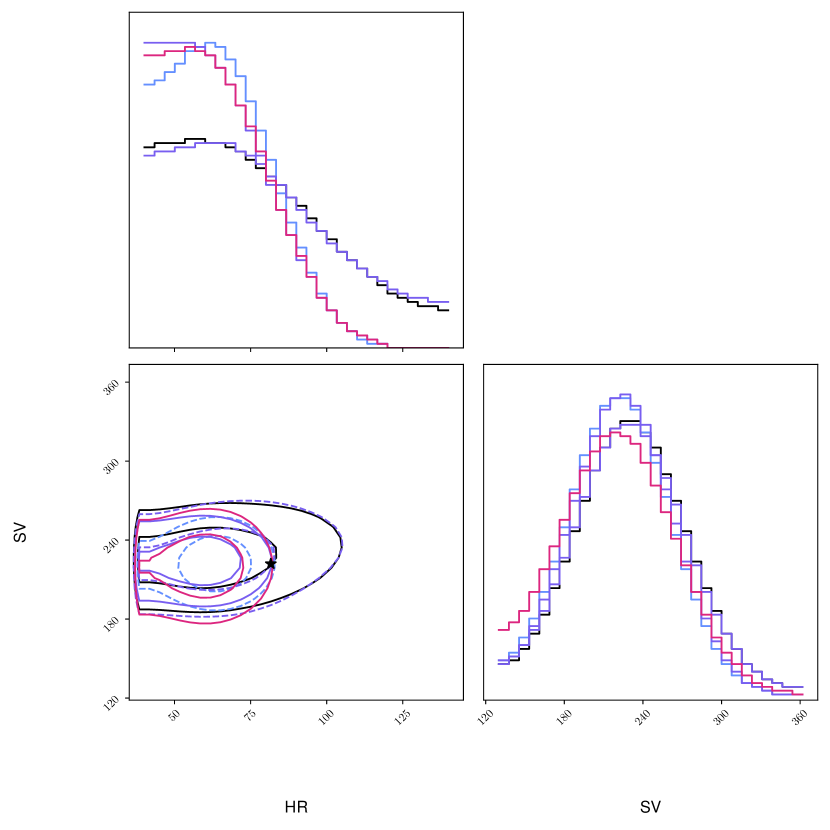
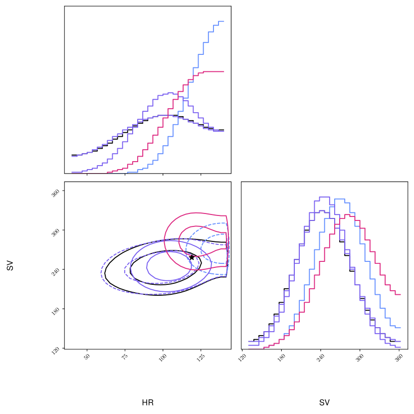
Figure 8: Three corner plots for task D with a calibration set with $50$ samples.

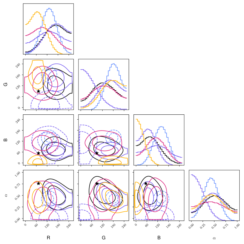
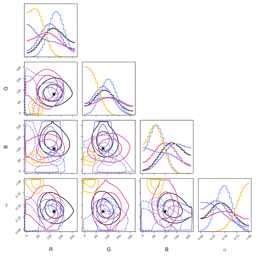
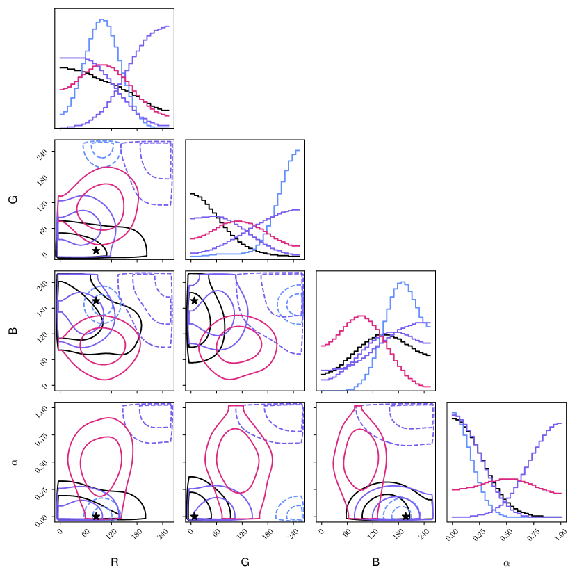
Figure 9: Three corner plots for task E with a calibration set with $50$ samples.

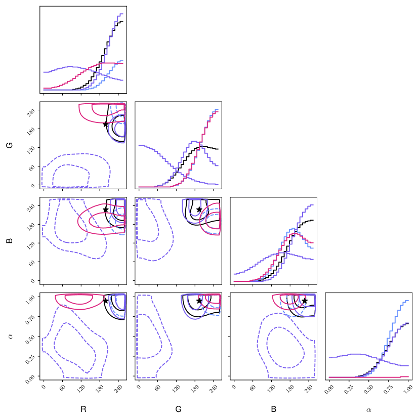
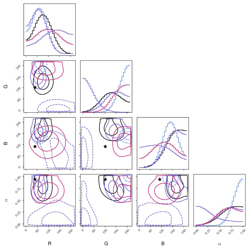
Figure 10: Three corner plots for task E with distribution shift with a calibration set with $50$ samples.

E.2 Calibration plots

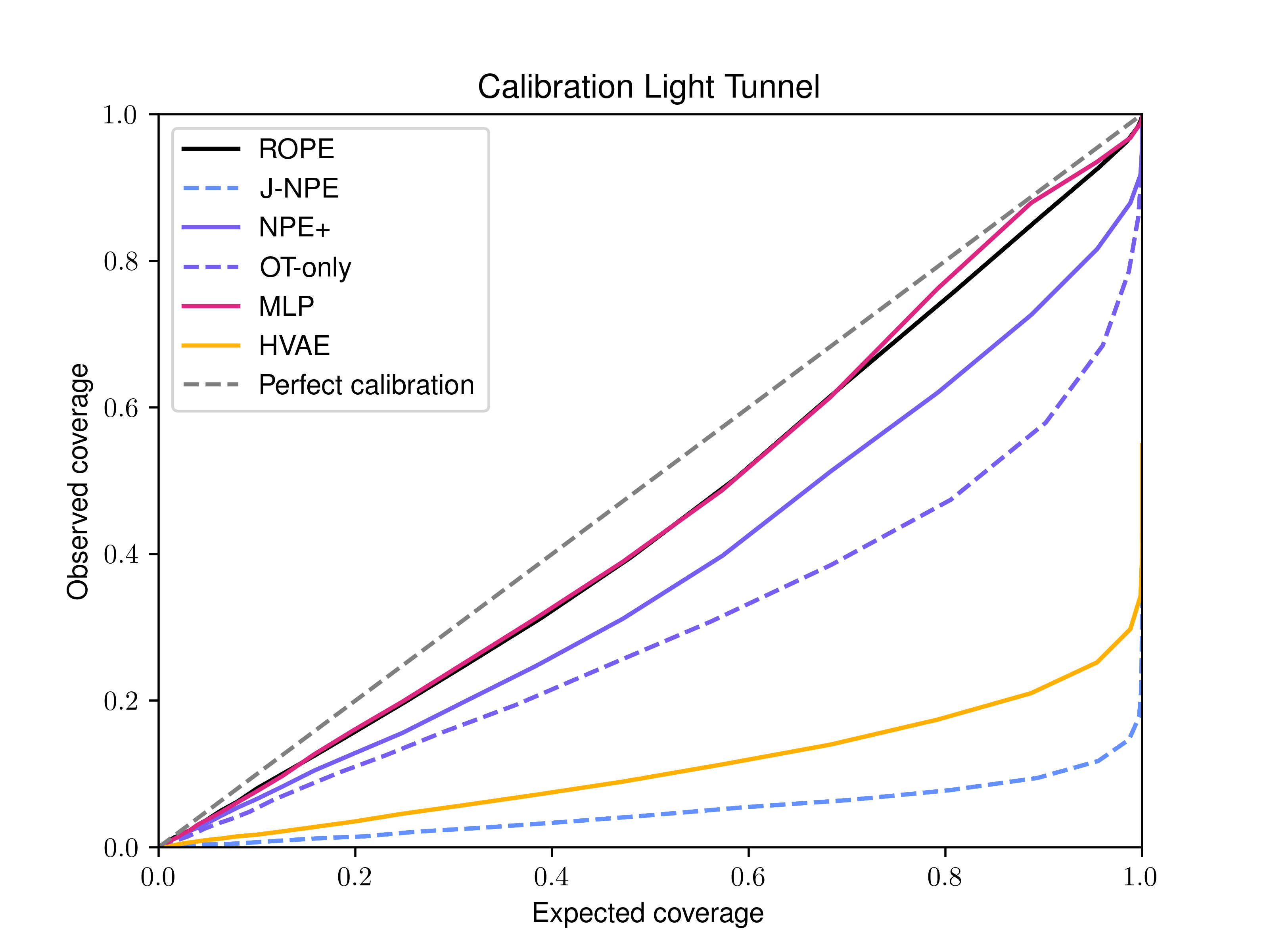
(a)

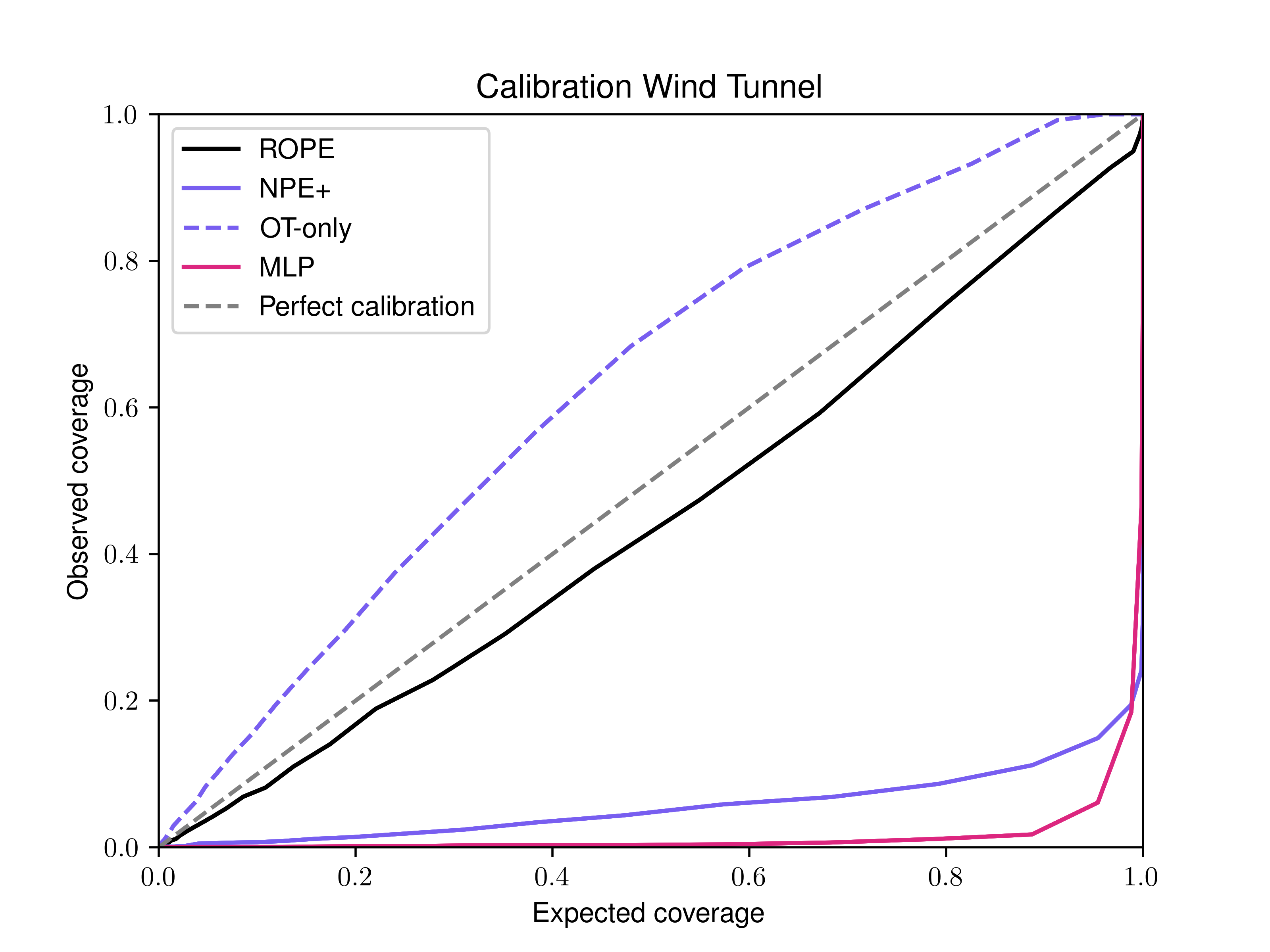
(b)

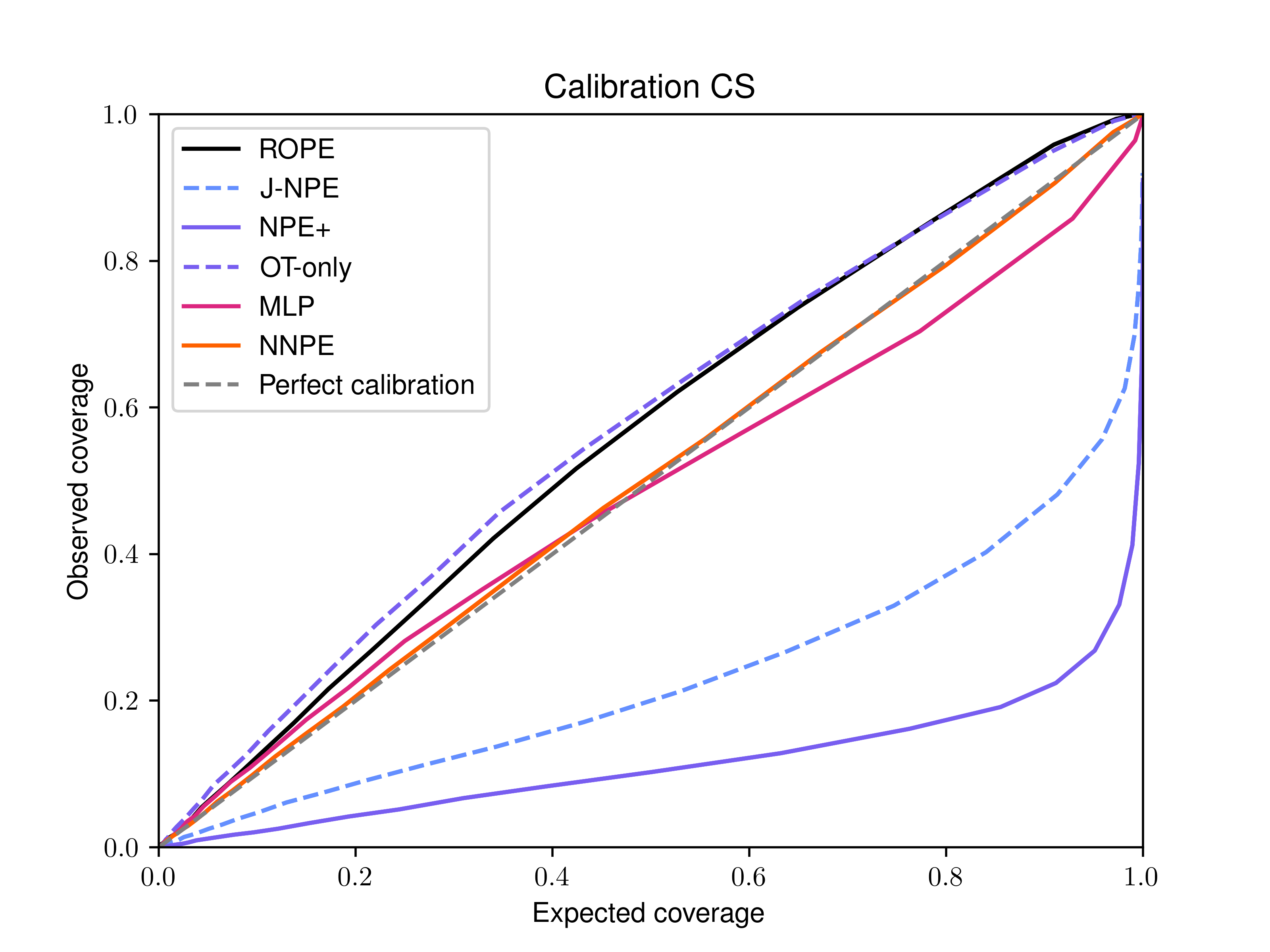
(c)

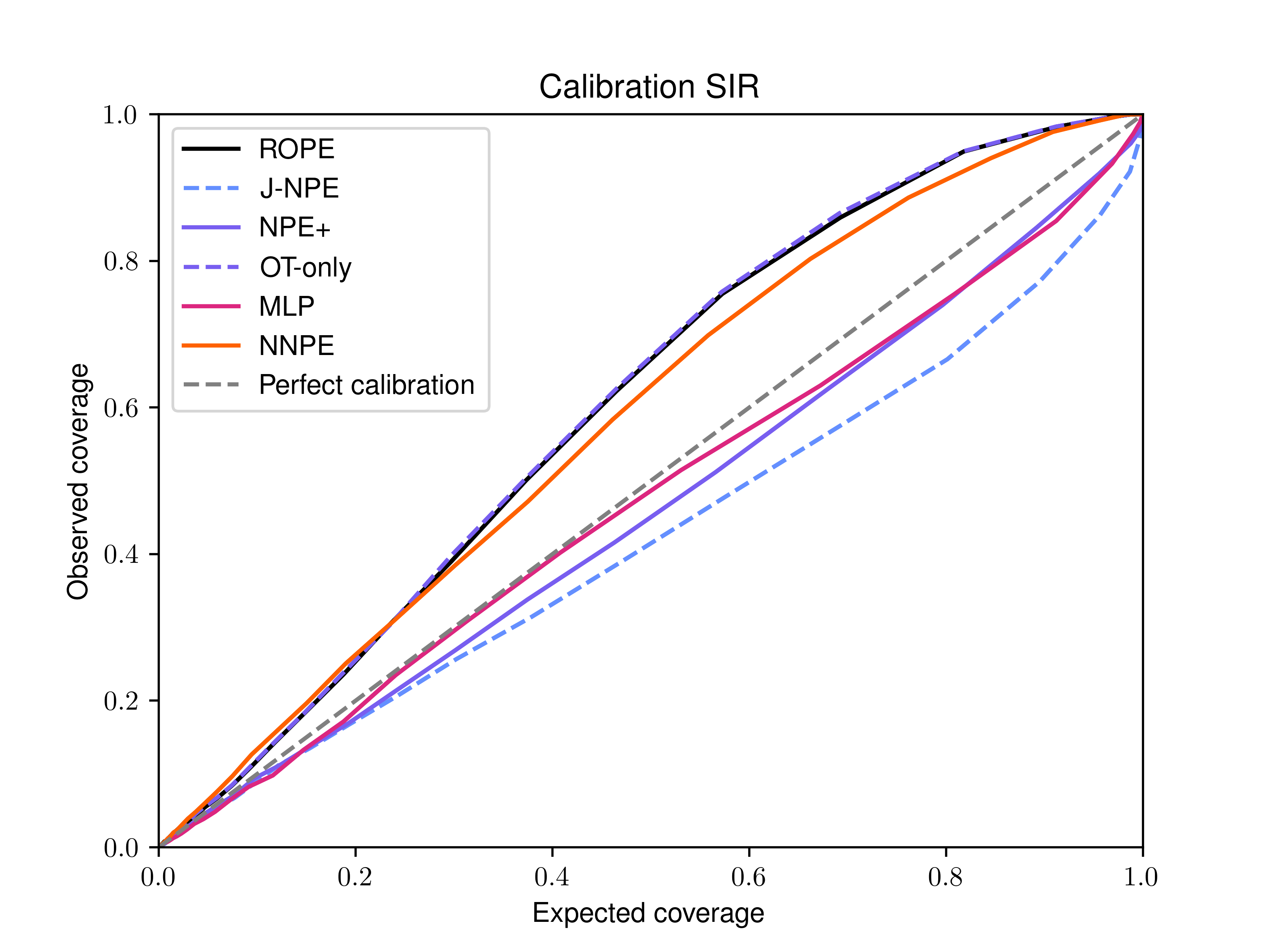
(d)

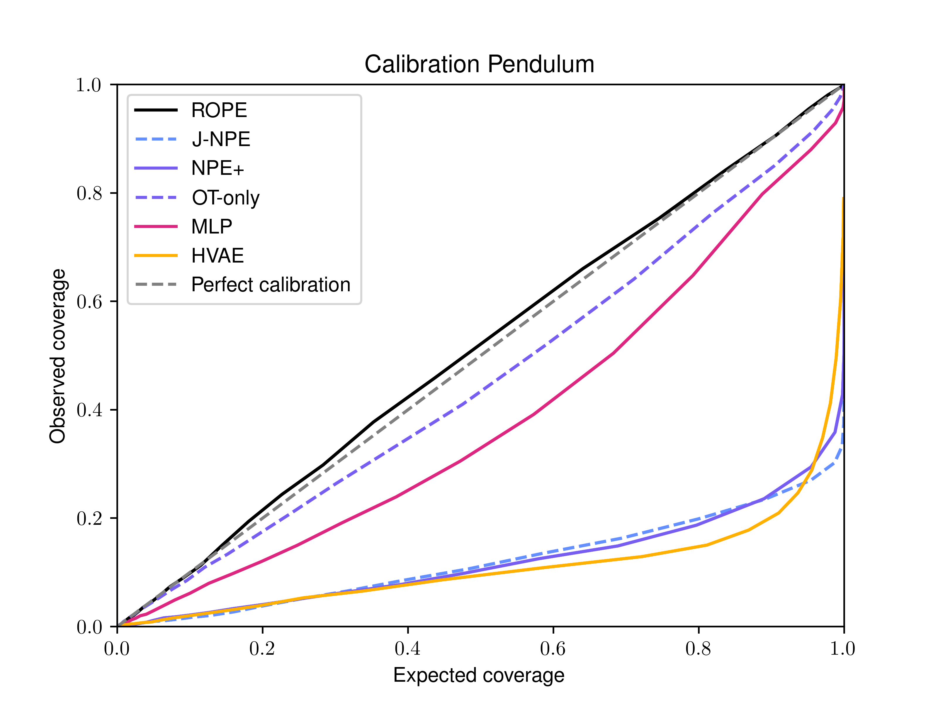
(e)

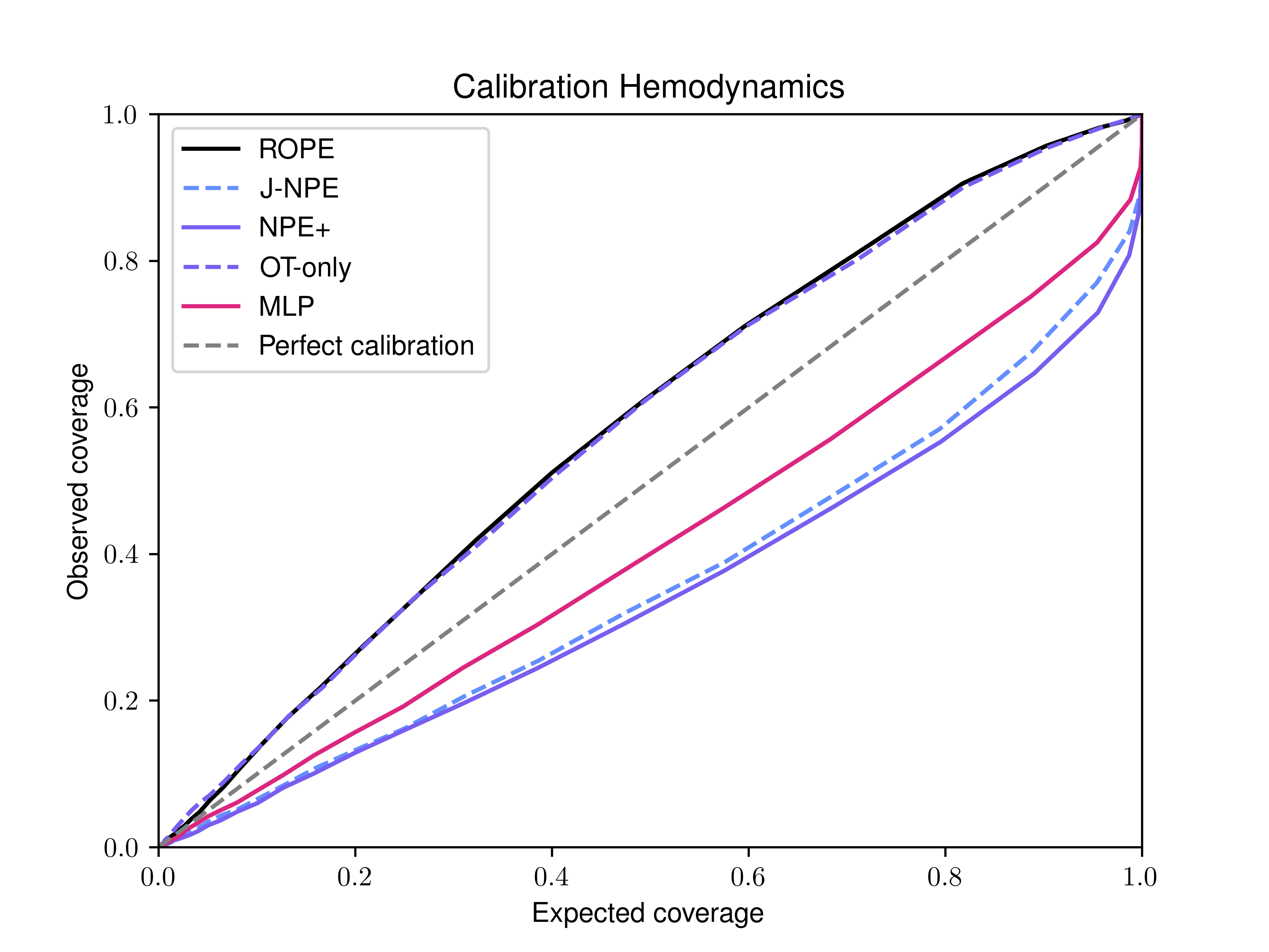
(f)

Figure 11: Calibration plots of the different methods on the 6 benchmarks, the coverage at each level is the average of the coverage of the marginal distributions. Each color indicates a different algorithm and the opacity is proportional to the size of the calibration set which ranges from $10$ to $1000$. We observe that ROPE and OT-only are consistently well calibrated for.

Appendix F Computing ACAUC

Algorithm 9 Statistical Calibration of Posterior Distribution

Input: Dataset of pairs $\mathcal{D}=\{(\theta^{i},\mathbf{x}^{i})\}$, Posterior estimator $\tilde{p}(\theta\mid\mathbf{x})$, Number of samples $N$.
Output: ACAUC

1:  $\text{AVG\_CALIBRATION}=0$

2:  for $k\in\{1,\dots,K\}$) do

3:     Initialize an empty list CredLevels

4:     for $(\theta^{i},\mathbf{x}^{i})\in\mathcal{D}$ do

5:        Initialize an empty list Samples

6:        for $j=1$ to $M$ do

7:           Sample $\theta^{j}$ from $\tilde{p}(\theta\mid\mathbf{x}^{i})$

8:           Append $\theta^{j}$ to Samples

9:        end for

10:        Sort Samples

11:        Compute the rank (position in ascending order) $r$ of $\theta$ in Samples

12:        Set $\text{CredLevels}=\frac{r}{N}$

13:        Append CredLevel to CredLevels

14:     end for

15:     Sort CredLevels

16:     $\text{CALIBRATION}=\sum_{i=1}^{N}\text{CredLevels}[i]-\frac{i}{N}$

17:     $\text{AVG\_CALIBRATION}=\text{AVG\_CALIBRATION}+\frac{\text{CALIBRATION}}{K}$

18:  end for

Return: AVG_CALIBRATION

Appendix G Learning Minimal Sufficient Statistics with Neural Posterior Estimation

We now discuss why NPE may learn a minimal sufficient statistic. First, under a sufficiently large validation set, NPE’s objective function is only optimal on the validation set if NPE models the true posterior as defined implicitly by the prior $p(\theta)$ and the likelihood corresponding to the simulator $S$. This consistency has been proven in (Papamakarios and Murray,, 2016) and is the motivation to use such an objective when estimating density. Second, some normalizing flows, such as autoregressive UMNN flows (Wehenkel and Louppe,, 2019), are universal approximators of continuous densities. In addition, neural networks are also universal function approximators. As such, we can claim that it is always possible to parameterize the NCDE $p_{\theta}(\theta\mid\mathbf{h}_{\omega}(\mathbf{x}))$ such that the class of functions its parameters represent contains the true posterior. We directly observe that $\mathbf{x}$ is only used by the NCDE through $\mathbf{h}_{\omega}(\mathbf{x})$. Thus, under perfect training $p_{\theta^{\star}}(\theta\mid\mathbf{h}_{\omega^{\star}}(\mathbf{x}))=p(\theta\mid\mathbf{x})$ and $\mathbf{h}_{\omega^{\star}}(\mathbf{x})$ is a sufficient statistic for $\theta$ given $\mathbf{x}$ under the simulator’s model.

Without additional constraint, we cannot claim anything about the minimality of $\mathbf{h}_{\omega^{\star}}(\mathbf{x})$. Nevertheless, we can enforce the neural network $\mathbf{h}_{\omega^{\star}}(\mathbf{x})$ has an information bottleneck and thus reduces the information carried. In practice, we ensure the output dimension of $\mathbf{h}_{\omega^{\star}}(\mathbf{x})$ and the NCDE achieves optimal performance on the test set. Recalling that, in the context of SBI, we can generate as many samples as needed and obtain estimators that closely approach the simulation’s posterior and a minimal sufficient statistic.

References

- Avecilla et al., (2022) Avecilla, G., Chuong, J. N., Li, F., Sherlock, G., Gresham, D., and Ram, Y. (2022). Neural networks enable efficient and accurate simulation-based inference of evolutionary parameters from adaptation dynamics. PLoS biology, 20(5):e3001633.
- Brehmer, (2021) Brehmer, J. (2021). Simulation-based inference in particle physics. Nature Reviews Physics, 3(5):305–305.
- Cannon et al., (2022) Cannon, P., Ward, D., and Schmon, S. M. (2022). Investigating the impact of model misspecification in neural simulation-based inference. arXiv preprint arXiv:2209.01845.
- Collett, (2005) Collett, E. (2005). Field guide to polarization. International society for optics and photonics.
- Cranmer et al., (2020) Cranmer, K., Brehmer, J., and Louppe, G. (2020). The frontier of simulation-based inference. Proceedings of the National Academy of Sciences, 117(48):30055–30062.
- Cuturi, (2013) Cuturi, M. (2013). Sinkhorn distances: Lightspeed computation of optimal transport. Advances in neural information processing systems, 26.
- Cuturi et al., (2022) Cuturi, M., Meng-Papaxanthos, L., Tian, Y., Bunne, C., Davis, G., and Teboul, O. (2022). Optimal transport tools (ott): A jax toolbox for all things wasserstein. arXiv preprint arXiv:2201.12324.
- Delaunoy et al., (2021) Delaunoy, A., Hermans, J., Rozet, F., Wehenkel, A., and Louppe, G. (2021). Towards reliable simulation-based inference with balanced neural ratio estimation. In Advances in Neural Information Processing Systems 2022.
- Delaunoy et al., (2020) Delaunoy, A., Wehenkel, A., Hinderer, T., Nissanke, S., Weniger, C., Williamson, A., and Louppe, G. (2020). Lightning-fast gravitational wave parameter inference through neural amortization. In Machine Learning and the Physical Sciences. Workshop at the 34th Conference on Neural Information Processing Systems (NeurIPS).
- Fatras et al., (2021) Fatras, K., Séjourné, T., Flamary, R., and Courty, N. (2021). Unbalanced minibatch optimal transport; applications to domain adaptation. In International Conference on Machine Learning, pages 3186–3197. PMLR.
- Gamella et al., (2024) Gamella, J. L., Bühlmann, P., and Peters, J. (2024). The causal chambers: Real physical systems as a testbed for AI methodology. arXiv preprint arXiv:2404.11341.
- Glöckler et al., (2022) Glöckler, M., Deistler, M., and Macke, J. H. (2022). Variational methods for simulation-based inference. In International Conference on Learning Representations 2022.
- Hashemi et al., (2022) Hashemi, M., Vattikonda, A. N., Jha, J., Sip, V., Woodman, M. M., Bartolomei, F., and Jirsa, V. K. (2022). Simulation-based inference for whole-brain network modeling of epilepsy using deep neural density estimators. medRxiv, pages 2022–06.
- Hermans et al., (2020) Hermans, J., Begy, V., and Louppe, G. (2020). Likelihood-free mcmc with amortized approximate ratio estimators. In International conference on machine learning, pages 4239–4248. PMLR.
- Huang et al., (2023) Huang, D., Bharti, A., Souza, A., Acerbi, L., and Kaski, S. (2023). Learning robust statistics for simulation-based inference under model misspecification. arXiv preprint arXiv:2305.15871.
- Linhart et al., (2022) Linhart, J., Rodrigues, P. L. C., Moreau, T., Louppe, G., and Gramfort, A. (2022). Neural posterior estimation of hierarchical models in neuroscience. In GRETSI 2022-XXVIIIème Colloque Francophone de Traitement du Signal et des Images.
- Lückmann, (2022) Lückmann, J.-M. (2022). Simulation-Based Inference for Neuroscience and Beyond. PhD thesis, Universität Tübingen.
- Lueckmann et al., (2021) Lueckmann, J.-M., Boelts, J., Greenberg, D., Goncalves, P., and Macke, J. (2021). Benchmarking simulation-based inference. In International Conference on Artificial Intelligence and Statistics, pages 343–351. PMLR.
- Lueckmann et al., (2017) Lueckmann, J.-M., Goncalves, P. J., Bassetto, G., Öcal, K., Nonnenmacher, M., and Macke, J. H. (2017). Flexible statistical inference for mechanistic models of neural dynamics. Advances in neural information processing systems, 30.
- Melis, (2017) Melis, A. (2017). Gaussian process emulators for 1d vascular models.
- Papamakarios and Murray, (2016) Papamakarios, G. and Murray, I. (2016). Fast -free inference of simulation models with bayesian conditional density estimation. Advances in neural information processing systems, 29.
- Papamakarios et al., (2021) Papamakarios, G., Nalisnick, E., Rezende, D. J., Mohamed, S., and Lakshminarayanan, B. (2021). Normalizing flows for probabilistic modeling and inference. The Journal of Machine Learning Research, 22(1):2617–2680.
- Papamakarios et al., (2019) Papamakarios, G., Sterratt, D., and Murray, I. (2019). Sequential neural likelihood: Fast likelihood-free inference with autoregressive flows. In The 22nd International Conference on Artificial Intelligence and Statistics, pages 837–848. PMLR.
- Peyré et al., (2017) Peyré, G., Cuturi, M., et al. (2017). Computational optimal transport. Center for Research in Economics and Statistics Working Papers.
- Rodrigues et al., (2022) Rodrigues, P. L., Statify, I., Arbel, M. N., Thoth, I., Forbes, F., and Mairal, J. (2022). Investigating model misspecification in simulation-based inference.
- Séjourné et al., (2019) Séjourné, T., Feydy, J., Vialard, F.-X., Trouvé, A., and Peyré, G. (2019). Sinkhorn divergences for unbalanced optimal transport. arXiv preprint arXiv:1910.12958.
- Tabak and Vanden-Eijnden, (2010) Tabak, E. G. and Vanden-Eijnden, E. (2010). Density estimation by dual ascent of the log-likelihood. Communications in Mathematical Sciences, 8(1):217–233.
- Takeishi and Kalousis, (2021) Takeishi, N. and Kalousis, A. (2021). Physics-integrated variational autoencoders for robust and interpretable generative modeling. Advances in Neural Information Processing Systems, 34:14809–14821.
- Tolley et al., (2023) Tolley, N., Rodrigues, P. L., Gramfort, A., and Jones, S. R. (2023). Methods and considerations for estimating parameters in biophysically detailed neural models with simulation based inference. bioRxiv, pages 2023–04.
- Villani et al., (2009) Villani, C. et al. (2009). Optimal transport: old and new, volume 338. Springer.
- Walker, (2013) Walker, S. G. (2013). Bayesian inference with misspecified models. Journal of statistical planning and inference, 143(10):1621–1633.
- Ward et al., (2022) Ward, D., Cannon, P., Beaumont, M., Fasiolo, M., and Schmon, S. (2022). Robust neural posterior estimation and statistical model criticism. Advances in Neural Information Processing Systems, 35:33845–33859.
- Wehenkel et al., (2022) Wehenkel, A., Behrmann, J., Hsu, H., Sapiro, G., Louppe, G., and Jacobsen, J.-H. (2022). Robust hybrid learning with expert augmentation. Transaction on Machine Learning Research.
- Wehenkel et al., (2023) Wehenkel, A., Behrmann, J., Miller, A. C., Sapiro, G., Sener, O., Cuturi, M., and Jacobsen, J.-H. (2023). Simulation-based inference for cardiovascular models. arXiv preprint arXiv:2307.13918.
- Wehenkel and Louppe, (2019) Wehenkel, A. and Louppe, G. (2019). Unconstrained monotonic neural networks. Advances in neural information processing systems, 32.