Beyond Scaling Laws: Understanding Transformer Performance with Associative Memory
Abstract
Increasing the size of a Transformer model does not always lead to enhanced performance. This phenomenon cannot be explained by the empirical scaling laws. Furthermore, improved generalization ability occurs as the model memorizes the training samples. We present a theoretical framework that sheds light on the memorization process and performance dynamics of transformer-based language models. We model the behavior of Transformers with associative memories using Hopfield networks, such that each transformer block effectively conducts an approximate nearest-neighbor search. Based on this, we design an energy function analogous to that in the modern continuous Hopfield network which provides an insightful explanation for the attention mechanism. Using the majorization-minimization technique, we construct a global energy function that captures the layered architecture of the Transformer. Under specific conditions, we show that the minimum achievable cross-entropy loss is bounded from below by a constant approximately equal to 1. We substantiate our theoretical results by conducting experiments with GPT-2 on various data sizes, as well as training vanilla Transformers on a dataset of 2M tokens.
1 Introduction
Transformer-based neural networks have exhibited powerful capabilities in accomplishing a myriad of tasks such as text generation, editing, and question-answering. These models are rooted in the Transformer architecture (Vaswani et al., 2017) which employs the self-attention mechanisms to capture the context in which words appear, resulting in superior ability to handle long-range dependencies and improved training efficiency. In many cases, models with more parameters result in better performance measured by perplexity (Kaplan et al., 2020), as well as in the accuracies of end tasks (Khandelwal et al., 2019; Rae et al., 2021; Chowdhery et al., 2023). As a result, larger and larger models are being developed in the industry. Recent models (Smith et al., 2022) can reach up to 530 billion parameters, trained on hundreds of billions of tokens with more than 10K GPUs.
Nevertheless, it is not always the case that bigger models result in better performance. For example, the 2B model MiniCPM (Hu et al., 2024) exhibits comparable capabilities to larger language models, such as Llama2-7B (Touvron et al., 2023), Mistral-7B (Jiang et al., 2023), Gemma-7B (Banks and Warkentin, 2024), and Llama-13B (Touvron et al., 2023). Moreover, as computational resources for training larger models increase, the size of available high-quality data may not keep pace. It has been documented that the generalization abilities of a range of models increase with the number of parameters and decrease when the number of training samples increases (Belkin et al., 2019; Nakkiran et al., 2021; d’Ascoli et al., 2020), indicating that generalization occurs beyond the memorization of training samples in over-parameterized neural networks (Power et al., 2022). Therefore, it is crucial to understand the convergence dynamics of training loss during memorization, both in relation to the model size and the dataset at hand. There has been an increasing interest in the empirical scaling laws under constraints on the training dataset size (Muennighoff et al., 2024). Let denote the number of the parameters of the model and denote the size of the dataset. Extensive experiments have led to the conclusion of the following empirical scaling laws (Kaplan et al., 2020) in terms of the model performance measured by the test cross-entropy loss on held-out data:
| (1) |
where are constants. Unfortunately, this scaling law does not explain why in many cases smaller models perform better.
In this paper, we focus on the theoretical aspects of the dependencies between the achievable performance, indicated by the pre-training loss, for transformer-based models, and the model and data sizes during memorization. It has been observed that a family of large language models tends to rely on knowledge memorized during training (Hsia et al., 2024), and the larger the models, the more they tend to encode the training data and organize the memory according to the similarity of textual context (Carlini et al., 2022; Tirumala et al., 2022). Therefore, we model the behavior of the Transformer layers with associative memory, which associates an input with a stored pattern, and inference aims to retrieve the related memories. A model for associative memory, known as the Hopfield network, was originally developed to retrieve stored binary-valued patterns based on part of the content (Amari, 1972; Hopfield, 1982). Recently, the classical Hopfield network has been generalized to data with continuous values. The generalized model, the Modern Continuous Hopfield Network (MCHN), has been shown to exhibit equivalence to the attention mechanism (Ramsauer et al., 2020). With MCHN, the network can store well-separated data points with a size exponential in the embedding dimension. However, the MCHN only explains an individual Transformer layer and relies heavily on regularization.
Transformer-based models consist of a stack of homogeneous layers. The attention and feed-forward layers contribute to the majority of the parameters and are also the key components of the attention mechanism. It has been shown that the feed-forward layers can be interpreted as persistent memory vectors, and the weights of the attention and feed-forward sub-layers can be merged into a new all-attention layer without compromising the model’s performance (Sukhbaatar et al., 2019). This augmentation enables a unified view that integrates the feed-forward layers into the attention layers, thereby significantly facilitating our analysis. Furthermore, the layered structure of the transformer networks induces a sequential optimization, reminiscent of the majorization-minimization (MM) technique (Ortega and Rheinboldt, 1970; Sun et al., 2016), which has been extensively utilized across domains such as signal processing and machine learning. Using the MM framework, we construct a global energy function tailored for the layered structure of the transformer network.
Our model provides a theoretical framework for analyzing the performance of transformer-based language models as they memorize training samples. Large language models only manifest capabilities for certain downstream tasks once the training loss reaches a specific threshold (Du et al., 2024). In practice, the training of large language models is terminated when the loss curves plateau. On the one hand, the validation loss offers valuable insights for budgetary considerations; it has been observed that even after training on up to 2T tokens, some models have yet to exhibit signs of saturation (Touvron et al., 2023). On the other hand, early stopping can potentially compromise the model’s generalization capabilities (Murty et al., 2023). On the other hand, implementing early stopping can potentially compromise the generalization capabilities of the models (Murty et al., 2023). We conduct a series of experiments utilizing GPT-2 across a spectrum of data sizes, concurrently training vanilla Transformer models on a dataset comprising 2M tokens. The experimental outcomes substantiate our theoretical results. We believe this work offers valuable theoretical perspectives on the optimal cross-entropy loss, which can inform and enhance decision-making regarding model training.
2 Related Work
Scaling laws
As discussed in the introduction, we have seen consistent empirical evidence that the performance of models increases as both the size of the models and the volume of training data scale up (Kaplan et al., 2020; Khandelwal et al., 2019; Rae et al., 2021; Chowdhery et al., 2023). Intensive experiments have also been conducted to explore neural scaling laws under various conditions, including constraints on computational budget (Hoffmann et al., 2022b), data (Muennighoff et al., 2024), and instances of over-training (Gadre et al., 2024). In these analyses, a decomposition of the expected risk is utilized, leading to the following fit:
| (2) |
For Chinchilla models, the fitted parameters are (Hoffmann et al., 2022a)
A line of research concerns the generalization of over-parameterized neural networks (Belkin et al., 2019; Nakkiran et al., 2021; Power et al., 2022). Recent experiments show that over-trained transformers exhibits inverted U-shaped scaling behavior (Murty et al., 2023), which cannot be explained by the empirical scaling laws.
Energy-based models
Energy-based models, motivated by statistical physics, have become a fundamental modeling tool in various fields of machine learning over the past few decades (LeCun et al., 2006). The central idea is to model the neural network through a parameterized probability density function for and to express the distribution in terms of a learnable energy function whose parameters correspond to the model’s parameters as
Here, is the normalizing constant known as the partition function.
Hopfield models
Classical Hopfield networks (Amari, 1972; Hopfield, 1982) were introduced as paradigmatic examples of associative memory. The network’s update dynamics define an energy function, whose fixed points correspond to the stored memories. An important indicator is the number of patterns that the model can memorize, known as the network’s storage capacity. Modifications to the energy function (Krotov and Hopfield, 2016; Demircigil et al., 2017) result in higher storage capacities (see Table 1 in Appendix A). The original model operates on binary variables. The modern continuous Hopfield network (MCHN) (Ramsauer et al., 2020) generalizes the Hopfield model to the continuous domain, making it an appealing tool for understanding the attention mechanism in Transformers, which also take vector embeddings in the real domain as inputs. Given an input (e.g., a prompt), the Hopfield layer retrieves a memory by converging to a local minimum of the energy landscape, and the update rule has a nice correspondence to the query-key-value mechanism in attention. Krotov (2021) proposes a Hierarchical Associative Memory (HAM) model that enables the description of the neural network with a global energy function, as opposed to energy functions for individual layers.
3 Model
We consider tokenized training samples where each element is a sequence of tokens whose length is bounded by a number Let be the set of held-out validation samples. The preprocessing of the dataset is described in Appendix D. The size of the dataset is proportional to the number of samples such that Let be the embedding dimension of the tokens, so each input sequence has dimensions. Let be the total number of parameters, most of which are attributed to the attention layers and the feed-forward layers. Then for some constant (see Appendix D). We use a generic distance metric in the Euclidean space.
3.1 Associative memories
We consider models trained with a causal language modeling objective. Given an input sequence of tokens the -layer Transformer outputs a distribution over the next token The transformer models are trained by maximizing the log-probability of the correct token given After training, the model develops the ability to generate desired content, such as predicting the correct continuations. Thus, the sequences can be viewed as patterns, as in the setting of associative memories, where stored patterns (e.g., sequences) can be retrieved using partial contents of the patterns. The tokenized patterns consist of a subset of the training samples based on the following observation.
Observation 1
The models tend to memorize the patterns of the training data.
Empirical studies on large language models have shown that the larger the models are, the more they tend to memorize training data (Carlini et al., 2022; Tirumala et al., 2022). This memorization allows the models to learn important patterns, such as world knowledge (Hsia et al., 2024), individual words (Chang and Bergen, 2022), and linguistic structure (Chang and Bergen, 2024). Therefore, we make the following assumption regarding memorization.
Assumption 1
After saturation, the model memorizes the training samples as patterns where for
To be economical with notations, we use to directly address the patterns By memorizing the samples, we mean that the patterns are stored within the model and can be retrieved when provided with an adequate prompt. Specifically, we follow the definitions in (Ramsauer et al., 2020) for stored and retrieved patterns.
Definition 1
For every pattern denote by an -ball such that The pattern is said to be stored if there exists a single fixed point to which all points converge, and for Such is said to be associated to the pattern and we denote The pattern is said to be retrieved if the converged point is -close to the fixed point
We also assume that the small set of held-out test samples exhibits the same patterns as those in the training set. In practice, the test samples are randomly selected from the same dataset as the training samples, preserving the distribution.
Assumption 2
Every element in the set of patterns associated with the test data is within for some Therefore, we assume
3.2 Transformer blocks
Transformers (Vaswani et al., 2017) are made of a stack of homogeneous layers, where each consists of a multi-head attention sub-layer, a feed-forward sub-layer, an add-norm operation with a skip connection, and layer normalization. As an example of a typical Transformer, the GPT-2 architecture is discussed in Appendix D. The multi-head attention and feed-forward (FF) layers account for most of the parameters in the model.
Attention mechanism
The attention mechanism arguably contributes most to the overall performance of the transformer models. The attention mechanism takes three matrices and as inputs that can be interpreted as keys, queries, and values. Setting facilitates the inclusion of residual connections. In a single update, an attention matrix is obtained using the update rule
Feed-forward layers
The FF layers take up almost two third of the model’s parameters. It has been shown that the FF layers operate essentially as key-value memories (Geva et al., 2020) such that where are parameter matrices and is a non-linear activation function such as ReLU. In fact, the FF layers can be merged into the attention without degrading the Transformer’s performance (Sukhbaatar et al., 2019). Thus, we have the following observation.
Observation 2
The attention layer and the feed-forward layer can be conceptually integrated into a unified transformer layer.
The attention layers and the FF layers contribute to the majority of the model’s parameters, such that the number of parameters is proportional to the square of the embedding dimension. The ratio depends on the number of layers and the hidden dimensions of the transformer blocks. In the current work, we do not consider other modifications such as lateral connections, skip-layer connections, or other compressive modules such as (Xiong et al., 2023; Fei et al., 2023; Munkhdalai et al., 2024).
4 A New Energy Function
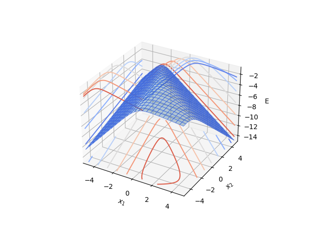
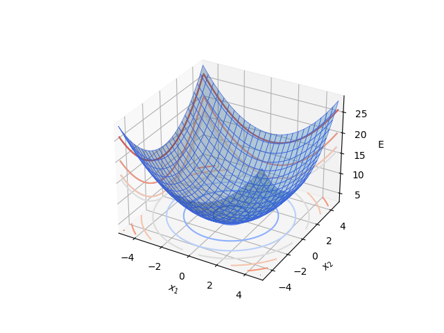
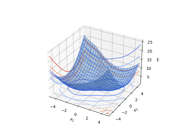
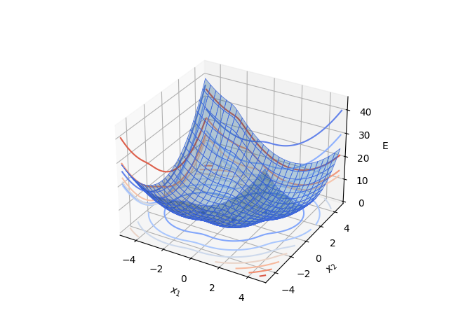
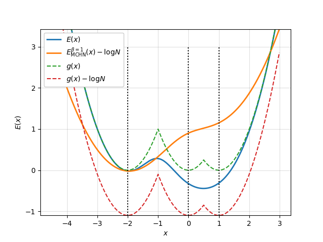
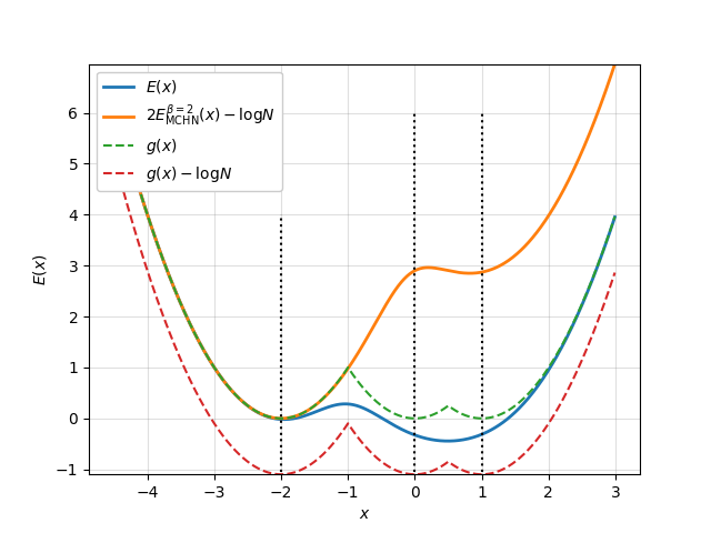
We first introduce a new energy function that does not rely on additional regularization terms. We then adapt this function to the layered transformer blocks using the majorization-minimization technique. For reference, related energy functions for Hopfield networks are listed in Table 1 within Appendix A. In particular, the energy function for the modern continuous Hopfield network (Ramsauer et al., 2020) is
Notice that the negative LogSumExp function was adapted from (Demircigil et al., 2017). However, in the continuous domain, the negative LogSumExp function is not convex, which makes it a less suitable candidate for the energy function. The MCHN energy then adds regularization terms to create a convex energy function. These regularization terms involve both the max norm of the input and the number of patterns.
Instead of designing different regularization terms, we define a new energy function through an auxiliary function
| (3) |
which functions as a nearest neighbor search over the the set of patterns So it holds that with if and only if According to Assumption 1, the model has memorized all the patterns; thus, the inference corresponds to a search algorithm based on some distance In the sequel, we use the squared Euclidean 2-norm for simplicity, although other norms could be used in general.
We consider a new energy function which also takes the form of LogSumExp. It is worth noting that the softmax function is the gradient of the LogSumExp function. By summing up the negative distance between and each stored pattern, the function assigns smaller values to points near the patterns. Our proposed energy function is
| (4) |
By replacing the dot product in the MCHN energy with a distance metric, achieves the same goal without additional regularization. As shown in Figures 1(a) and 1(b), as an extension of (Demircigil et al., 2017), the negative LogSumExp is not convex in the real domain, so regularization terms are applied. Figures 1(d) and 1(c) show that the landscape of the proposed energy resembles that of the MCHN energy. In (Ramsauer et al., 2020), it is shown that induces stationary points near the stored patterns. Here, the proposed function serves as a smooth surrogate of the desired function in Eq. (3), therefore also demonstrates the retrieval ability.
Proposition 1
Given the proposed energy satisfies
The proof of Proposition 1 is due to Lemma 3 and is postponed to Appendix B. Furthermore, we show that is close to the MCHN energy.
Proposition 2
Let we have
The proof is given in Appendix B. Fig. 1 provides visualizations of the two propositions using one-dimensional patterns. The following result follows directly from the above inequalities.
Proposition 3
Since the proposed energy and the MCHN energy both approximate the search for the nearest pattern (desired stationary point), according to Theorem 4 in (Ramsauer et al., 2020), in each transformer layer, the probability density of the transformer layer, corresponding to the retrieval, is
where is the normalizing factor and is as defined in Definition 1. We assume that is centered at the -th pattern. We make the following assumption on the samples in order to study the memorization. In practice, this requires the training dataset to be of very good quality.
Assumption 3
The patterns in are well-separated, i.e.,
Under Assumption 3, the energy function, confined in can be replaced by the nearest neighbor search So we can make the following claim.
Claim 1
Suppose the patterns are well-separated, then the probability density is
| (5) |
4.1 The layered structure
Previous Hopfield models could only handle a single hidden layer, whereas Transformers often consist of a stack of homogeneous blocks of attention and FF layers. To model the multi-layered structure of Transformers, we employ a technique known as majorization-minimization (MM) (Ortega and Rheinboldt, 1970; Sun et al., 2016), which aims to accelerate optimization using surrogate convex functions. We argue that the layered structure serves the same purpose when the patterns memorized by all layers encompass the set of training samples.
We divide the set of samples into where Then, the energy function for each layer can be written as
Denote by the embedding vector input into the first transformer layer and the output of the -th layer for Let be the energy function associated with the Hopfield model of the -th layer, then the sequential structure of the transformer network is achieved by forwarding the output to the -th layer as input, i.e.,
| (6) | ||||
where the retrieved fix point attractor in the -th layer is -close to in for some Such sequential optimization step is equivalent to the MM technique where every minimization step locally approximates the objective function. In particular, Eq. (6) corresponds to the surrogate function Eq. in (Sun et al., 2016). Therefore, we define a global energy function
| (7) |
is continuous but not convex. As opposed to the HAM (Krotov, 2021), the global energy function is not a linear combination of the component energies. According to Lemma 3, we have
| (8) |
So
as in Eq. in (Sun et al., 2016). The probability density function corresponding to the layered transformer network can then be written as
| (9) |
where denotes the model’s parameters and is the normalizing constant.
Remark 1
If the model is severely over-parameterized, the energy function can approximate the energy of the sample distribution well and is not confined to the form expressed in Eq. (9).
5 Cross-Entropy Loss
We now proceed to analyze the loss of Transformer networks. The cross-entropy loss, which measures the difference between predicted probabilities and actual labels, is commonly used for training Transformer models. The attention mechanism includes a softmax operation that outputs a probability distribution In practice, the final softmax output is then fed into a task-specific layer for downstream tasks, such as predictions and classifications. Thus, we compare the last softmax output of the transformer blocks with the target distribution.
We demonstrate that the cross-entropy loss can be formulated using the log partition function of the model’s distribution, which reflects how the attention weights are allocated based on the patterns. Let us consider the cross-entropy loss on the test dataset Generally, the cross-entropy loss is the negative log-likelihood computed over a mini-batch. Since we are considering un-batched validation samples, the loss is normalized by the size
According to Eq. (8), there exist a layer such that is close to i.e.,
| (10) |
for some such that We further assume that is constant. Under Assumption 1, the target distribution, which encodes all the patterns in , is given by
where is the Dirac delta function such that and is the probability mass assigned to pattern for Suppose the data points are homogeneous, i.e., then and the corresponding test samples induces the distribution
| (11) |
We have the following result regarding the cross-entropy loss.
Proposition 4
Let be the cross-entropy loss of the above model, then
where
The proof is deferred to Appendix C.1. Note that the empirically obtained loss function Eq. (2) for the Chinchilla model converges to as and which substantiates our theory that with minimum obtained when
Remark 2
The cross-entropy can be written as
When the model is severely over-parameterized, the energy function can well approximate the energy of the sample distribution. In this case, the minimal cross-entropy equals the entropy of the training samples.
Next, we take a closer look at the layer partition function. We have
| (12) |
where is due to Appendix C.2, is the radius of According to Lemma 5, we have
where
is the hyper-volume of the -dimensional ball of radius Note that the volume of the unit ball in higher dimensions decreases fast with respect to the increase in dimensionality. The gamma function can be approximated using Stirling’s approximation for large values of its argument. Applying Stirling’s approximation to the gamma function in the denominator of the volume formula for large , we get:
For to have a volume of , the radius must be approximately asymptotically. Bringing to Eq. (5), we get
| (13) |
In Section 3, we argue that
Therefore, for to reach we need
In Table 2 in Appendix A, we compare the reported cross-entropy loss of various transformer-based models in the literature. Usually, a family of models ranging in a variety of sizes is reported, and we select the largest ones. We observe that similar cross-entropy loss is achieved across a wide range of architectural shapes (including depth, width, attention heads, FF dimensions, and context lengths). Nevertheless, the losses all satisfy
Remark 3
We remark that some models add auxiliary regularization terms such as the z-loss (Chowdhery et al., 2023; Yang et al., 2023) during their training. In these cases, the scaling laws should take into consideration the additional terms. Also, modifications to the transformer blocks, such as additional layer normalization may contribute to the lower bound of the cross-entropy.
6 Empirical Results
We explore the hypothesis regarding the radius in Section 5 using a pre-trained GPT-2 medium model. Additionally, we train various GPT-2 small models and vanilla Transformer models to analyze their cross-entropy losses.
6.1 Empirical evaluation of the radius
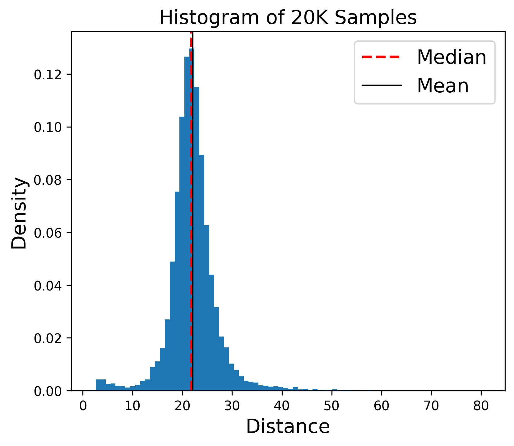
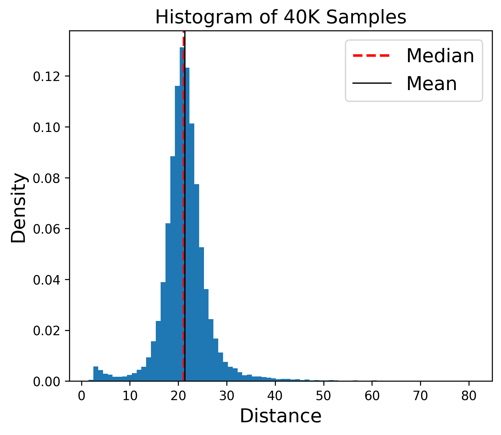
We evaluate the radius in of a pre-trained GPT-2 medium model. We use the 24-layer pre-trained GPT-2 model (Radford et al., 2019)111available at https://github.com/openai/gpt-2. The medium size model has 355M parameters. The model is pre-trained with a causal language modeling objective (next sentence prediction) on a very large (40 GB) text corpus extracted from web pages. The hidden dimension
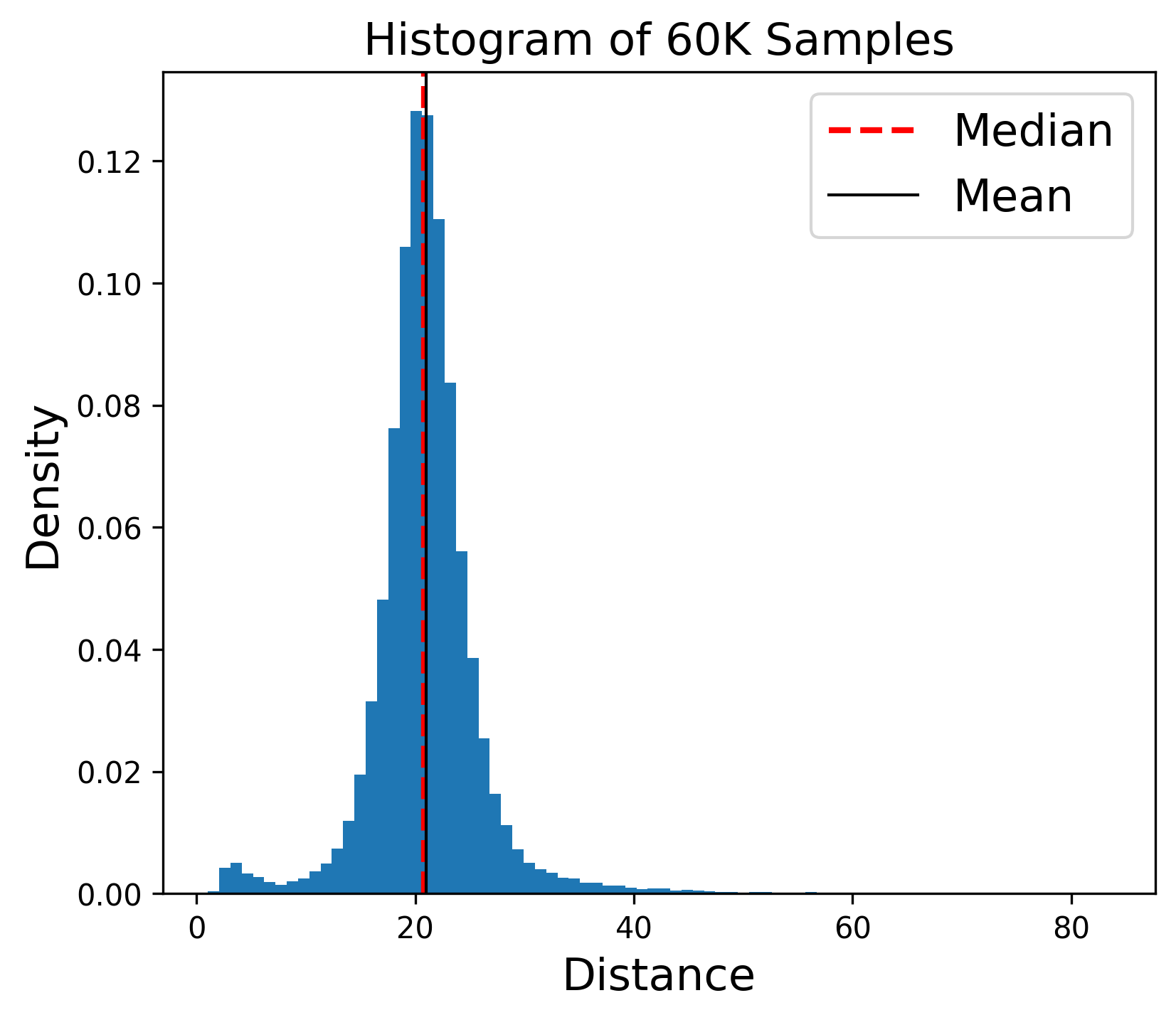
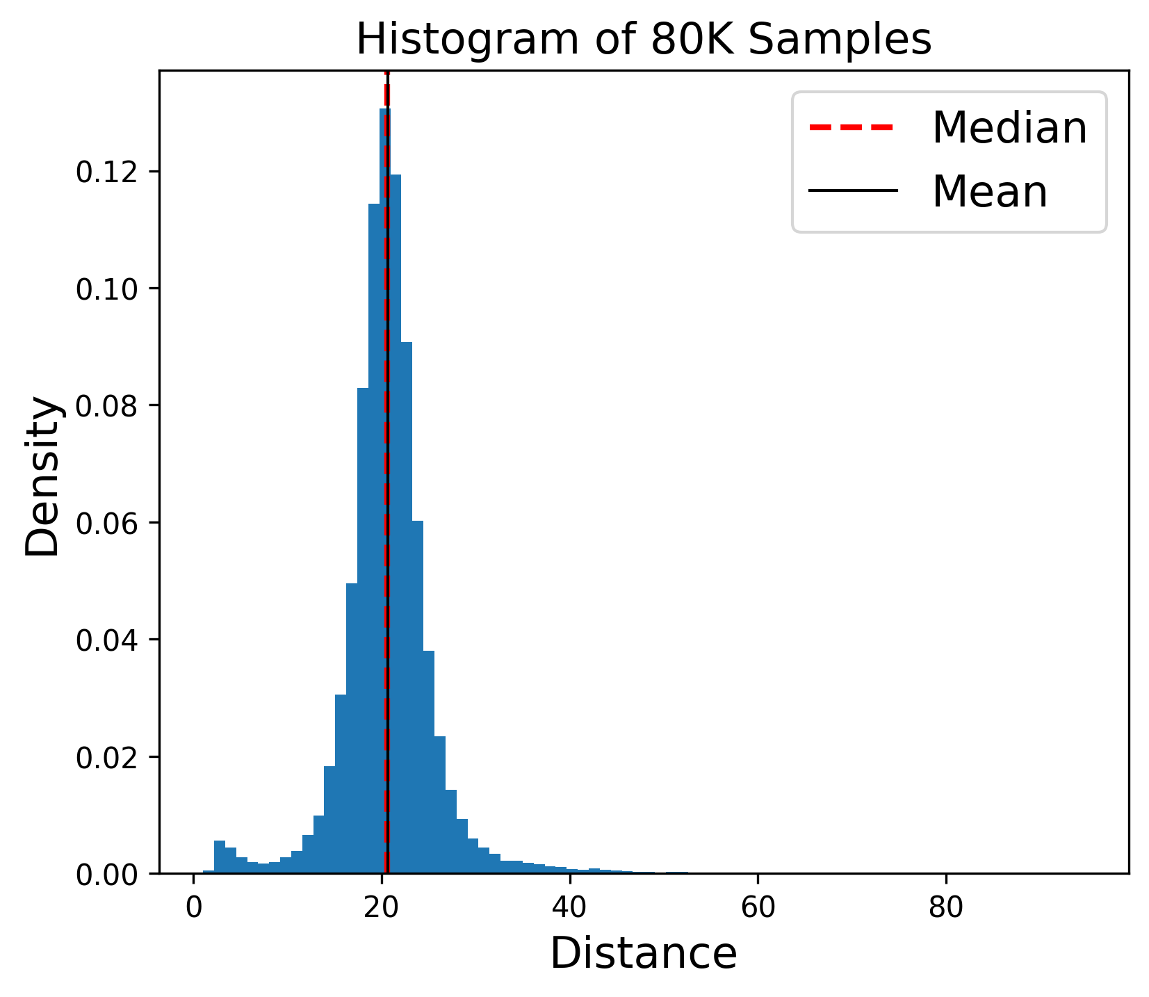
We test the model on the OpenWebText (Gokaslan and Cohen, 2019) dataset which is a reproduction of the WebText dataset used for training the GPT-2 model. The dataset contains 9B tokens from 8,013,769 documents. We randomly sample K chunks of tokens from the dataset. These cover approximately of the documents and constitute approximately of the tokens used for training. For each sample chunk, we record the activation vector of the last layer for prediction of the next token. Since the GPT-2 model is causal, the activation depends on all activations of earlier sequences. As discussed above, each vector should be close to a stored pattern We find the distance between each activation vector and its nearest neighbor in terms of the norm. In Fig. 2, we plot the histogram of the nearest neighbor distances for these output activations using and of the output vectors. In all these cases, the mean and median are approximately 20, so that a typical of pattern has radius This corroborates our theory in Eq. (13) in Section 5, according to which the radius is of order Note that the activation is only collected for of the documents, the estimated radius may be greater than actual one in the model.
6.2 Training GPT-2
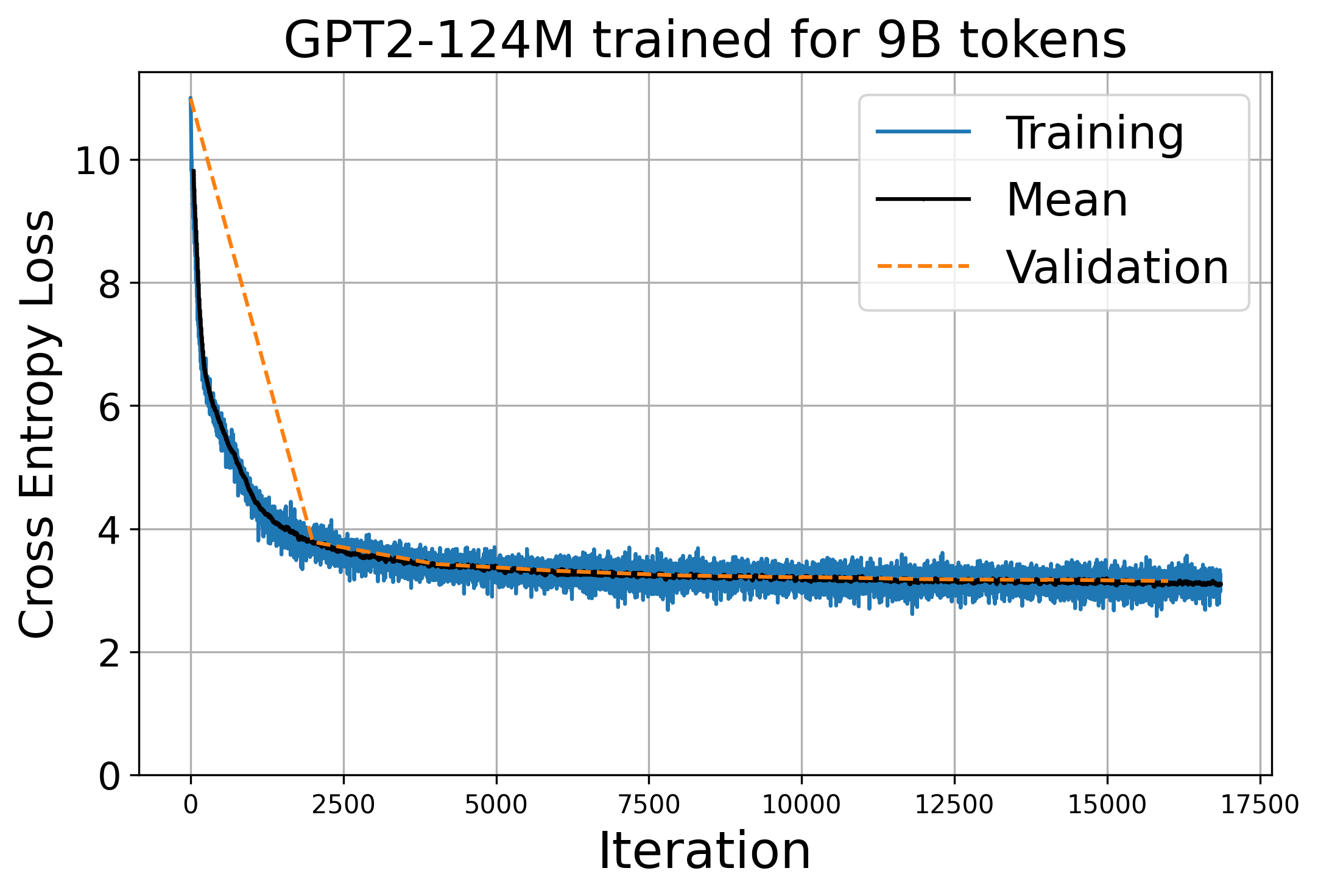
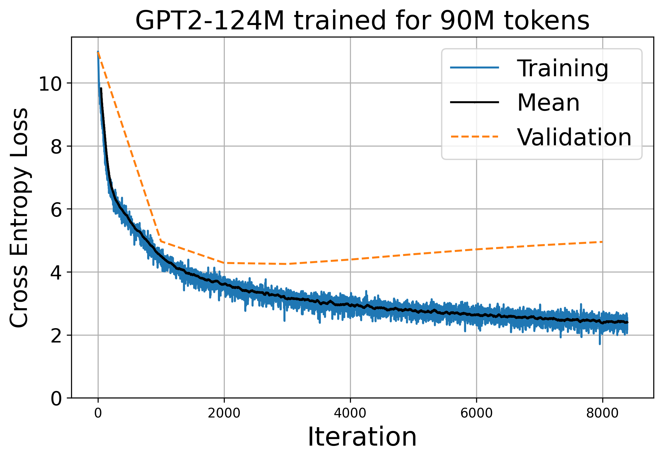
We train a 12-layer transformer language model with the GPT-2 small tokenizer and architecture () on the publicly available OpenWebText dataset (Gokaslan and Cohen, 2019), a reproduction of the WebText dataset used for training the original GPT-2 model, which contains 9B tokens from 8,013,769 documents
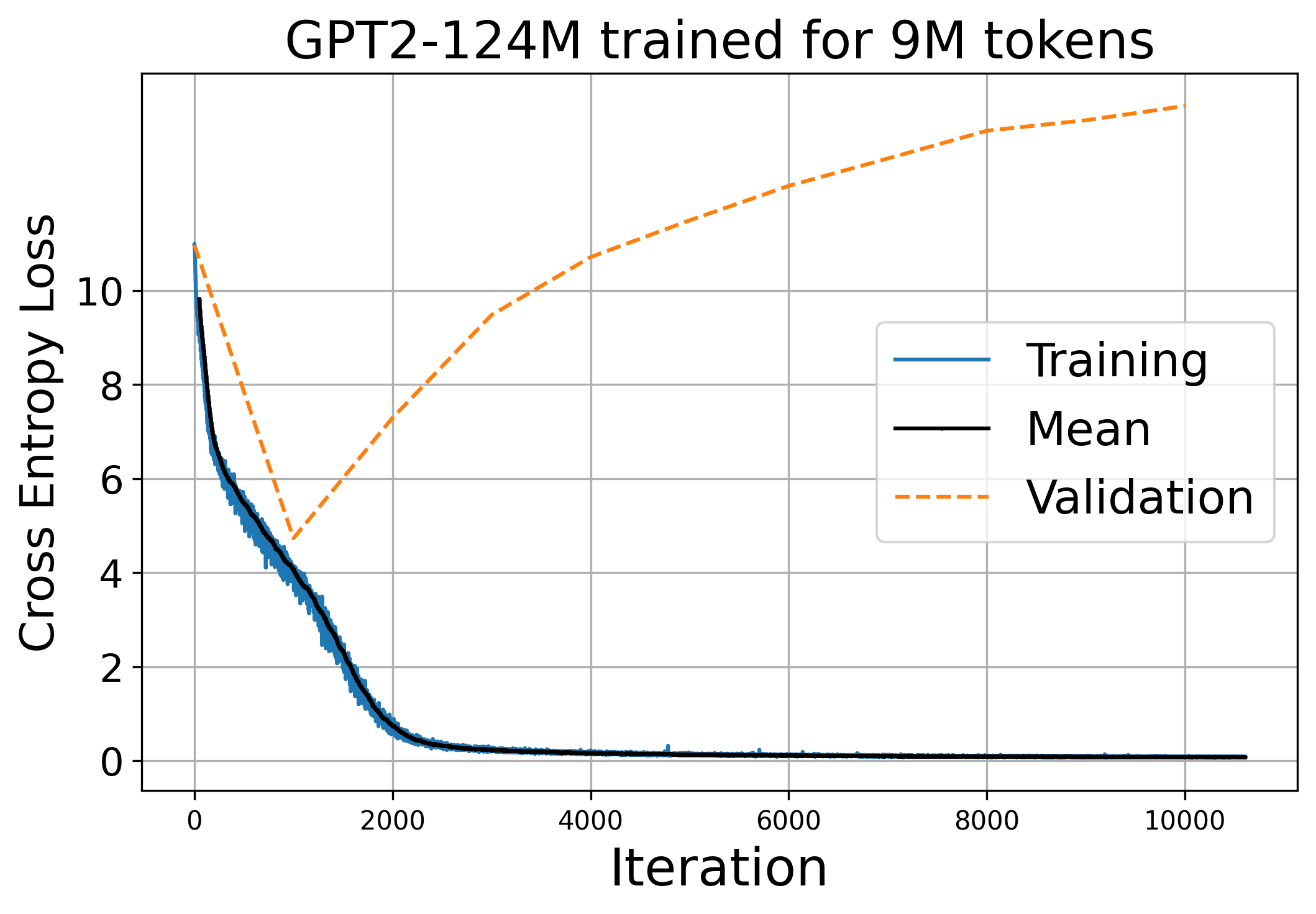
We train three models using different amount of data. We create subsets containing the first (90M) and (9M) of the OpenWebText data, and then train over a typical training time. For all the settings, we split the dataset into a training set and a smaller test set. We use a batch-size of 12 on the training set and evaluate the cross-entropy loss on the test set. The training and test cross-entropy losses are reported in Fig. 3. The training with (9M) of the OpenWebText data clearly experiences over-fitting, and the training loss vanishes over iterations. This is because the training samples are not well-separated so the energy of the model reduces to the summation of some delta functions and no longer satisfies Eq. (5). When training with 90M tokens and 9B tokens, the training cross-entropy losses are both above 2. Since the model size is about the order when trained on 90M tokens, the model can achieve similar training loss and validation loss compared to the setting with 9B tokens.
6.3 Training Vanilla Transformers
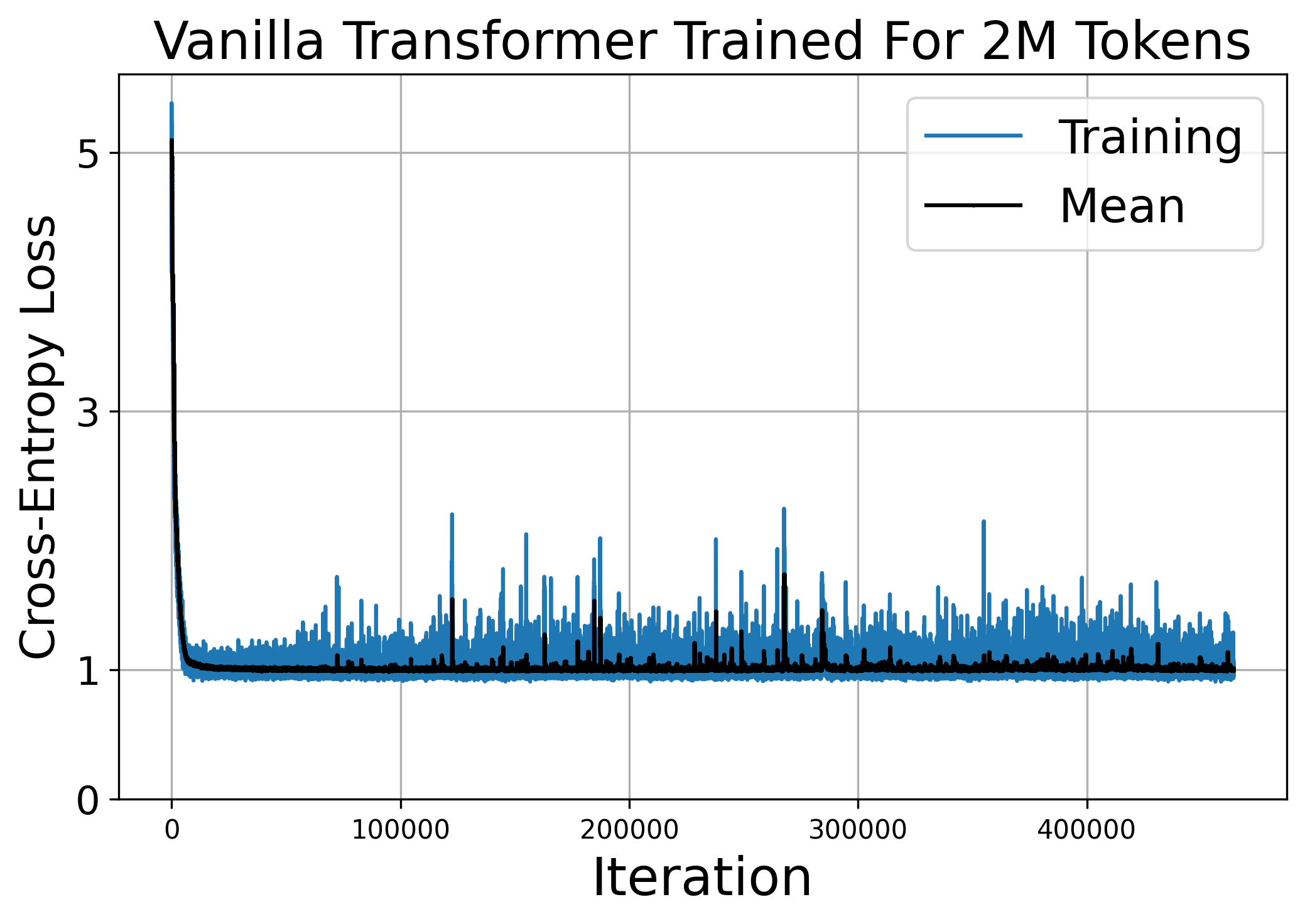
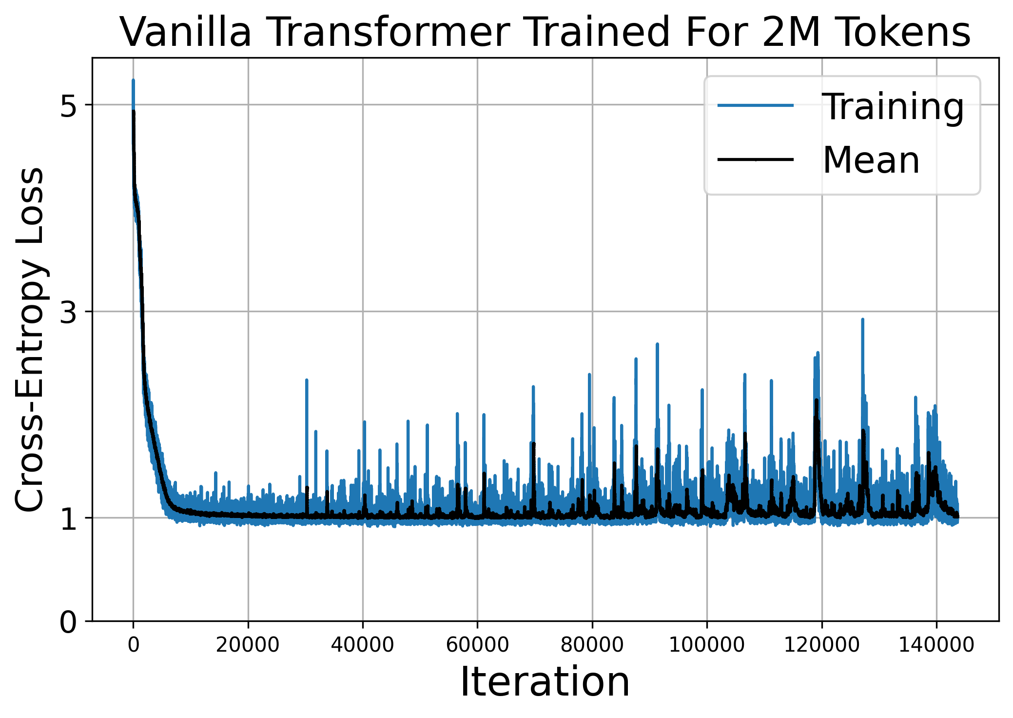
We next train vanilla transformer models using a small amount of high-quality data. The of Question-Formation dataset, proposed by McCoy et al. (2020), consists of pairs of English sentences in declarative formation and their corresponding question formation. The dataset contains M tokens. The sentences are context-free with a vocabulary size of 68 words, and the task is to convert declarative sentences into questions.
We follow the settings in (Murty et al., 2023) to train two vanilla Transformers () with layers and layers respectively. We use a batch size of 8 and tie the input and output matrices as done in (Press and Wolf, 2017). The training losses are shown in Fig. 4, where the losses stabilize at a value of around 1 as predicted in Proposition 4.
7 Conclusion
We model transformer-based networks with associative memory and study the cross-entropy loss with respect to model and data sizes. By proposing a new energy function in Eq. 5, which does not rely on additional regularization terms as is common in modern continuous Hopfield networks, we demonstrate that the proposed energy function corresponds to a nearest neighbor search across patterns memorized during training. We then construct a global energy function for the layered structure of the transformer models using the majorization-minimization technique.
In practice, we have observed that the majority of transformer models tend to achieve a cross-entropy loss of approximately 2.2. The optimal balance between model and data sizes, however, is often determined by the collective expertise of practitioners. Additionally, the performance of these models can be compromised by both early and delayed stopping.
We believe the current paper represents an important step towards understanding the convergence and generalization behaviors of large transformer models. It provides insights into the theoretically optimal cross-entropy loss, which can inform both budgetary planning and model termination strategies.
Acknowledgments
The author thanks Dr. Yongqi Xu for stimulating discussions and practical assistance with the experiments.
Appendix A Deferred Tables
| Reference | Domain | Energy | Capacity |
|---|---|---|---|
| Hopfield (1982) | |||
| Krotov and Hopfield (2016) | |||
| Demircigil et al. (2017) | |||
| Ramsauer et al. (2020) | |||
| Model | Model Size | Data Size | Reference | |
|---|---|---|---|---|
| Transformer | B | B | (Kaplan et al., 2020) | |
| Chinchilla | B | T | (Hoffmann et al., 2022a) | |
| PaLM 2 | B | B | (Anil et al., 2023) | |
| GPT-2 | B | B | (Muennighoff et al., 2024) | |
| MiniCPM | B | B | (Hu et al., 2024) |
Appendix B Some Properties of the Energy Functions
We introduce some useful properties of the LogSumExp function defined below. This is particularly useful because The softmax function, widely utilized in the Transformer models, is the gradient of the LogSumExp function. As shown in (Grathwohl et al., 2019), the LogSumExp corresponds to the energy function of the a classifier.
Lemma 1
is convex.
Proof
Lemma 2
Suppose then we have
Proof Taking log on each side of the inequality
yields the results.
Consequently, we have the following smooth approximation for the min function.
Lemma 3
Suppose then we have
Lemma 4
For we have
where
Proof Let
According to the mean value theorem, such that
So
B.1 Proof of Proposition 2
Appendix C Deferred Proofs from Section 5
C.1 Proof of Proposition 4
C.2
Let denote the -ball with radius centered at be the hyper-volume of the -dimensional unit sphere,
be the (incomplete) gamma functions. Then
Lemma 5
The incomplete gamma function satisfies
Proof For we have
Integrating from 0 to on each side yields the result.
Theorem C.1 (Stirling’s approximation)
For any complex the Stirling’s approximation gives that
For large
Appendix D Transformer Details: Using GPT-2 as an Example
The original GPT-2 model was trained on a 40GB large dataset called WebText that is made of data derived from outbound links from Reddit. The model is trained on the next sentence prediction (NSP) task in a self-supervised manner. A pre-trained tokenizer can be applied to convert the text into tokens using a fixed vocabulary. A max token length (e.g., ) is set, so during training, if the number of tokens is greater than the documents will be truncated. The model is trained causally, which means that the prediction for the next token only depends on the inputs from earlier tokens. The model was trained with a global batch size of 512, and the test perplexity still improves if given more training time.
GPT-2 uses a byte-level version of Byte Pair Encoding (BPE), and the vocabulary size is . The hidden dimension for the medium size model is . So the input sequence is of dimension. These sequences are passed through the model. For the medium size model, these include 24 transformer encoder blocks with 1024 hidden units and 16 self-attention heads (i.e., ). The number of parameters in the multi-head attention layer is The number of parameters in the dense weights and layer normalization is and the number of parameters in the feed-forward weight matrices and bias is with As we can observe, the multi-head attention and feed-forward layers account for most of the parameters in the model, and with some constant in this case.
The loss used for the GPT-2 model is the log-probability of a dataset divided by the number of canonical units (e.g., a character, a byte, a word), which is equivalent to the cross-entropy loss. The cross-entropy loss is commonly used to measure the divergence between the predicted probabilities and the true labels. For the NSP task, the model is trained to predict the next token in a sequence based on the context of the previous tokens. So the cross-entropy is taken between the predicted probabilities of the token and the labels’ probabilities for all tokens in the vocabulary, i.e.,
Another commonly used loss is the perplexity, which is equivalent to the exponentiated version of the cross-entropy.
References
- Amari (1972) S.-I. Amari. Learning patterns and pattern sequences by self-organizing nets of threshold elements. IEEE Transactions on Computers, 100(11):1197–1206, 1972.
- Anil et al. (2023) R. Anil, A. M. Dai, O. Firat, M. Johnson, D. Lepikhin, A. Passos, S. Shakeri, E. Taropa, P. Bailey, Z. Chen, et al. Palm 2 technical report. arXiv preprint arXiv:2305.10403, 2023.
- Banks and Warkentin (2024) T. W. J. Banks and T. Warkentin. Gemma: Introducing new state-of-the-art open models, 2024.
- Belkin et al. (2019) M. Belkin, D. Hsu, S. Ma, and S. Mandal. Reconciling modern machine-learning practice and the classical bias–variance trade-off. Proceedings of the National Academy of Sciences, 116(32):15849–15854, 2019.
- Carlini et al. (2022) N. Carlini, D. Ippolito, M. Jagielski, K. Lee, F. Tramer, and C. Zhang. Quantifying memorization across neural language models. In The Eleventh International Conference on Learning Representations, 2022.
- Chang and Bergen (2022) T. A. Chang and B. K. Bergen. Word acquisition in neural language models. Transactions of the Association for Computational Linguistics, 10:1–16, 2022.
- Chang and Bergen (2024) T. A. Chang and B. K. Bergen. Language model behavior: A comprehensive survey. Computational Linguistics, pages 1–58, 2024.
- Chowdhery et al. (2023) A. Chowdhery, S. Narang, J. Devlin, M. Bosma, G. Mishra, A. Roberts, P. Barham, H. W. Chung, C. Sutton, S. Gehrmann, et al. Palm: Scaling language modeling with pathways. Journal of Machine Learning Research, 24(240):1–113, 2023.
- d’Ascoli et al. (2020) S. d’Ascoli, L. Sagun, and G. Biroli. Triple descent and the two kinds of overfitting: Where & why do they appear? Advances in Neural Information Processing Systems, 33:3058–3069, 2020.
- Demircigil et al. (2017) M. Demircigil, J. Heusel, M. Löwe, S. Upgang, and F. Vermet. On a model of associative memory with huge storage capacity. Journal of Statistical Physics, 168:288–299, 2017.
- Du et al. (2024) Z. Du, A. Zeng, Y. Dong, and J. Tang. Understanding emergent abilities of language models from the loss perspective. arXiv preprint arXiv:2403.15796, 2024.
- Fei et al. (2023) W. Fei, X. Niu, P. Zhou, L. Hou, B. Bai, L. Deng, and W. Han. Extending context window of large language models via semantic compression. arXiv preprint arXiv:2312.09571, 2023.
- Gadre et al. (2024) S. Y. Gadre, G. Smyrnis, V. Shankar, S. Gururangan, M. Wortsman, R. Shao, J. Mercat, A. Fang, J. Li, S. Keh, et al. Language models scale reliably with over-training and on downstream tasks. arXiv preprint arXiv:2403.08540, 2024.
- Geva et al. (2020) M. Geva, R. Schuster, J. Berant, and O. Levy. Transformer feed-forward layers are key-value memories. arXiv preprint arXiv:2012.14913, 2020.
- Gokaslan and Cohen (2019) A. Gokaslan and V. Cohen. Openwebtext corpus. http://Skylion007.github.io/OpenWebTextCorpus, 2019.
- Grathwohl et al. (2019) W. Grathwohl, K.-C. Wang, J.-H. Jacobsen, D. Duvenaud, M. Norouzi, and K. Swersky. Your classifier is secretly an energy based model and you should treat it like one. In International Conference on Learning Representations, 2019.
- Hoffmann et al. (2022a) J. Hoffmann, S. Borgeaud, A. Mensch, E. Buchatskaya, T. Cai, E. Rutherford, D. d. L. Casas, L. A. Hendricks, J. Welbl, A. Clark, et al. Training compute-optimal large language models. arXiv preprint arXiv:2203.15556, 2022a.
- Hoffmann et al. (2022b) J. Hoffmann, S. Borgeaud, A. Mensch, E. Buchatskaya, T. Cai, E. Rutherford, D. de Las Casas, L. A. Hendricks, J. Welbl, A. Clark, et al. An empirical analysis of compute-optimal large language model training. Advances in Neural Information Processing Systems, 35:30016–30030, 2022b.
- Hopfield (1982) J. J. Hopfield. Neural networks and physical systems with emergent collective computational abilities. Proceedings of the National Academy of Sciences, 79(8):2554–2558, 1982.
- Hsia et al. (2024) J. Hsia, A. Shaikh, Z. Wang, and G. Neubig. Ragged: Towards informed design of retrieval augmented generation systems. arXiv preprint arXiv:2403.09040, 2024.
- Hu et al. (2024) S. Hu, Y. Tu, X. Han, C. He, G. Cui, X. Long, Z. Zheng, Y. Fang, Y. Huang, W. Zhao, et al. Minicpm: Unveiling the potential of small language models with scalable training strategies. arXiv preprint arXiv:2404.06395, 2024.
- Jiang et al. (2023) A. Q. Jiang, A. Sablayrolles, A. Mensch, C. Bamford, D. S. Chaplot, D. d. l. Casas, F. Bressand, G. Lengyel, G. Lample, L. Saulnier, et al. Mistral 7b. arXiv preprint arXiv:2310.06825, 2023.
- Kaplan et al. (2020) J. Kaplan, S. McCandlish, T. Henighan, T. B. Brown, B. Chess, R. Child, S. Gray, A. Radford, J. Wu, and D. Amodei. Scaling laws for neural language models. arXiv preprint arXiv:2001.08361, 2020.
- Khandelwal et al. (2019) U. Khandelwal, O. Levy, D. Jurafsky, L. Zettlemoyer, and M. Lewis. Generalization through memorization: Nearest neighbor language models. arXiv preprint arXiv:1911.00172, 2019.
- Krotov (2021) D. Krotov. Hierarchical associative memory. arXiv preprint arXiv:2107.06446, 2021.
- Krotov and Hopfield (2016) D. Krotov and J. J. Hopfield. Dense associative memory for pattern recognition. Advances in Neural Information Processing Systems, 29, 2016.
- LeCun et al. (2006) Y. LeCun, S. Chopra, R. Hadsell, M. Ranzato, and F. Huang. A tutorial on energy-based learning. Predicting Structured Data, 1(0), 2006.
- McCoy et al. (2020) R. T. McCoy, R. Frank, and T. Linzen. Does syntax need to grow on trees? sources of hierarchical inductive bias in sequence-to-sequence networks. Transactions of the Association for Computational Linguistics, 8:125–140, 2020.
- Muennighoff et al. (2024) N. Muennighoff, A. Rush, B. Barak, T. Le Scao, N. Tazi, A. Piktus, S. Pyysalo, T. Wolf, and C. A. Raffel. Scaling data-constrained language models. Advances in Neural Information Processing Systems, 36, 2024.
- Munkhdalai et al. (2024) T. Munkhdalai, M. Faruqui, and S. Gopal. Leave no context behind: Efficient infinite context transformers with infini-attention. arXiv preprint arXiv:2404.07143, 2024.
- Murty et al. (2023) S. Murty, P. Sharma, J. Andreas, and C. D. Manning. Grokking of hierarchical structure in vanilla transformers. arXiv preprint arXiv:2305.18741, 2023.
- Nakkiran et al. (2021) P. Nakkiran, G. Kaplun, Y. Bansal, T. Yang, B. Barak, and I. Sutskever. Deep double descent: Where bigger models and more data hurt. Journal of Statistical Mechanics: Theory and Experiment, 2021(12):124003, 2021.
- Ortega and Rheinboldt (1970) J. Ortega and W. Rheinboldt. Iterative Solution of Nonlinear Equations in Several Variables, volume 30. SIAM, 1970.
- Power et al. (2022) A. Power, Y. Burda, H. Edwards, I. Babuschkin, and V. Misra. Grokking: Generalization beyond overfitting on small algorithmic datasets. arXiv preprint arXiv:2201.02177, 2022.
- Press and Wolf (2017) O. Press and L. Wolf. Using the output embedding to improve language models. In Proceedings of the 15th Conference of the European Chapter of the Association for Computational Linguistics: Volume 2, Short Papers, pages 157–163, 2017.
- Radford et al. (2019) A. Radford, J. Wu, R. Child, D. Luan, D. Amodei, and I. Sutskever. Language models are unsupervised multitask learners. 2019.
- Rae et al. (2021) J. W. Rae, S. Borgeaud, T. Cai, K. Millican, J. Hoffmann, F. Song, J. Aslanides, S. Henderson, R. Ring, S. Young, et al. Scaling language models: Methods, analysis & insights from training gopher. arXiv preprint arXiv:2112.11446, 2021.
- Ramsauer et al. (2020) H. Ramsauer, B. Schäfl, J. Lehner, P. Seidl, M. Widrich, L. Gruber, M. Holzleitner, T. Adler, D. Kreil, M. K. Kopp, et al. Hopfield networks is all you need. In International Conference on Learning Representations, 2020.
- Smith et al. (2022) S. Smith, M. Patwary, B. Norick, P. LeGresley, S. Rajbhandari, J. Casper, Z. Liu, S. Prabhumoye, G. Zerveas, V. Korthikanti, et al. Using deepspeed and megatron to train megatron-turing NLG 530b, a large-scale generative language model. arXiv preprint arXiv:2201.11990, 2022.
- Sukhbaatar et al. (2019) S. Sukhbaatar, E. Grave, G. Lample, H. Jegou, and A. Joulin. Augmenting self-attention with persistent memory. arXiv preprint arXiv:1907.01470, 2019.
- Sun et al. (2016) Y. Sun, P. Babu, and D. P. Palomar. Majorization-minimization algorithms in signal processing, communications, and machine learning. IEEE Transactions on Signal Processing, 65(3):794–816, 2016.
- Tirumala et al. (2022) K. Tirumala, A. Markosyan, L. Zettlemoyer, and A. Aghajanyan. Memorization without overfitting: Analyzing the training dynamics of large language models. Advances in Neural Information Processing Systems, 35:38274–38290, 2022.
- Touvron et al. (2023) H. Touvron, L. Martin, K. Stone, P. Albert, A. Almahairi, Y. Babaei, N. Bashlykov, S. Batra, P. Bhargava, S. Bhosale, et al. Llama 2: Open foundation and fine-tuned chat models. arXiv preprint arXiv:2307.09288, 2023.
- Vaswani et al. (2017) A. Vaswani, N. Shazeer, N. Parmar, J. Uszkoreit, L. Jones, A. N. Gomez, Ł. Kaiser, and I. Polosukhin. Attention is all you need. Advances in neural information processing systems, 30, 2017.
- Xiong et al. (2023) W. Xiong, J. Liu, I. Molybog, H. Zhang, P. Bhargava, R. Hou, L. Martin, R. Rungta, K. A. Sankararaman, B. Oguz, et al. Effective long-context scaling of foundation models. arXiv preprint arXiv:2309.16039, 2023.
- Yang et al. (2023) A. Yang, B. Xiao, B. Wang, B. Zhang, C. Bian, C. Yin, C. Lv, D. Pan, D. Wang, D. Yan, et al. Baichuan 2: Open large-scale language models. arXiv preprint arXiv:2309.10305, 2023.