The physical mechanism behind magnetic field alignment in interstellar clouds

Abstract

Context. A tight correlation between interstellar clouds contours and their local magnetic field orientation has been widely observed. However, the physical mechanisms responsible for this correlation remain unclear.

Aims. We investigate the alignment mechanism between the magnetic field and interstellar clouds.

Methods. We perform three- and two-dimensional MHD simulations of warm gas streams in the thermally-bistable atomic interstellar medium (ISM) colliding with velocities of the order of the velocity dispersion in the ISM. In these simulations, we follow the evolution of magnetic field lines, identify and elucidate the physical processes causing their evolution.

Results. The collision produces a fast MHD shock, and a condensation front roughly one cooling length behind it, on each side of the collision front. A cold dense layer forms behind the condensation front, onto which the gas settles, decelerating smoothly. We find that the magnetic field lines, initially oriented parallel to the flow direction, are perturbed by the fast MHD shock, across which the magnetic field fluctuations parallel to the shock front are amplified. The downstream perturbations of the magnetic field lines are further amplified by the compressive downstream velocity gradient between the shock and the condensation front caused by the settlement of the gas onto the dense layer. This mechanism causes the magnetic field to become increasingly parallel to the dense layer, and the development of a shear flow around the latter. Furthermore, the bending-mode perturbations on the dense layer are amplified by the non-linear thin-shell instability (NTSI), stretching the density structures formed by the thermal instability, and rendering them parallel to the bent field lines. By extension, we suggest that a tidal stretching velocity gradient such as that produced in gas infalling into a self-gravitating structure must straighten the field lines along the accretion flow, orienting them perpendicular to the density structures. We also find that the upstream superalfvénic regime transitions to a transalfvénic regime between the shock and the condensation front, and then to a subalfvénic regime inside the condensations. Finally, in two-dimensional simulations with a curved collision front, the presence of the magnetic field inhibits the generation of turbulence by the shear around the dense layer.

Conclusions. Our results provide a feasible physical mechanism for the observed transition from parallel to perpendicular relative orientation of the magnetic field and the density structures as the density structures become increasingly dominated by self-gravity.

1 Introduction

Studying the role of magnetic fields in the formation and evolution of atomic and molecular clouds (MCs) has been an important research topic for both observational and theoretical astronomy. Magnetic fields are thought to be an important ingredient in the dynamics of the ISM, providing a possible support mechanism against gravitational collapse, and guiding the gas flow in the surroundings of filamentary structures, among many other effects. In addition, a tight correlation between the orientation of the magnetic field and cold atomic clouds (CACs) has been identified in the last decade. For example, Clark et al. (2015) found that the plane of the sky magnetic field, measured using polarized thermal dust emission, is aligned with atomic hydrogen structures detected with HI emission and Clark et al. (2014) also observed a similar alignment in HI fibers, which are thin long dense structures identified in HI emission using the Rolling Hough transform. In addition, Planck Collaboration et al. (2016a) found that the plane of the sky magnetic field, detected using polarized thermal dust emission, is aligned with molecular structures traced by dust, and Planck Collaboration et al. (2016b) found that the relative orientation of the projected magnetic field and dust filaments changes from parallel to perpendicular when sampling higher density regions in nearby MCs. Skalidis et al. (2022) studied the role of the magnetic field in the transition between $\mathrm{H{I}-H_{2}}$ using multiple tracers to investigate the gas properties of Ursa Minor. They found that turbulence is transalfvénic and that the gas probably accumulates along magnetic field lines and generates overdensities where molecular gas can form.

However, the origin of these alignments remains unclear, as most of the observational evidence refers to spatial and orientation correlations without a clear understanding of the causality involved. Therefore, it is crucial to understand the interplay between the precursors of molecular clouds (MCs) and magnetic fields. Since CACs are thought to constitute the primordial place for the early stages of the evolution of molecular clouds and, eventually, star-forming regions (e.g., Koyama & Inutsuka, 2002; Audit & Hennebelle, 2005; Vázquez-Semadeni et al., 2006; Heitsch et al., 2006; Heiner et al., 2015; Seifried et al., 2017), understanding the alignment mechanism of magnetic field lines in CACs is relevant to elucidate the role of magnetic fields in the formation of MCs and star formation.

To study this correlation statistically, Soler et al. (2013) proposed the histogram of relative orientations (HRO) and found that the relative orientation of the magnetic field and isodensity contours changes from parallel to perpendicular in a high magnetization ($\beta=0.1$) computer-simulated cloud. This change of orientation was studied in Soler & Hennebelle (2017) with an analytic approach where the authors found the parallel or anti-parallel ($\phi=0^{\circ},180^{\circ}$) and perpendicular ($\phi=90^{\circ}$) configurations are equilibrium points. Therefore, they argue, the system tends to evolve to these $\phi$ values.

More recently, Seifried et al. (2020) investigated the relative orientation of magnetic field and three- and two-dimensional projected structures using synthetic dust polarization maps. They found that the magnetic field changes its orientation from parallel to perpendicular at $n\approx 10^{2}-10^{3}\mbox{\,cm}^{-3}$ in regions where the mass-to-flux ratio has values close to or below 1. In addition, they found that projection effects due to the relative orientation between the cloud and the observer affect the measurements.

The relative orientation of the magnetic field alignment with CACs is, arguably, intrinsically related to the formation mechanism of CACs. The formation of cold atomic clouds (CACs) by colliding flows with pure hydrodynamic was studied in Heitsch et al. (2006), where the authors performed simulations of colliding warm neutral gas streams, including the multi-phase nature of the ISM and not considering gravity nor magnetic fields. They discussed three important instabilities that might play a role in the formation of CACs: the thermal instability (TI), the Kelvin-Helmholtz instability (KHI), and the non-linear thin-shell instability (NTSI). They concluded that these instabilities break up the coherent flows, seeding small-scale density perturbations necessary for gravitational collapse and thus star formation.

Hennebelle (2013) studied the formation of non-self-gravitating CACs in the ISM. This author focused on finding the mechanism responsible for the elongation of CACs and concluded that the clouds are generated by the stretching induced by turbulence because they are aligned with the strain. Moreover, the author also found that the Lorentz force confines CACs. Inoue & Inutsuka (2016), in agreement with the previous work, found that the strain is also the origin of the magnetic field alignment with fibers in HI clouds formed in a shock-compressed layer using simulations resembling the local bubble. More recently, Gazol & Villagran (2021) studied the morphology of CACs in forced magnetized and hydrodynamical simulations, finding that the presence of the magnetic field increases the probability of filamentary CACs.

A consequence of the supersonic gas streams forming CACs is the formation of shocks. Shocks form wherever there are supersonic velocity differences between two nearby regions. Since the velocity dispersions in the neutral ISM are supersonic, shocks are ubiquitous in the ISM, which, in general, produce density fluctuations of various amplitudes.

The formation of CACs out of the warm neutral medium (WNM) in the Galactic ISM requires strong cooling in addition to the presence of shocks. Such cooling often causes TI (Field, 1965; Pikel’Ner, 1968; Field et al., 1969), and in general produces large density jumps without the need for very strongly supersonic flows (Vázquez-Semadeni et al., 1996, 2006).

In the presence of supersonic flows and cooling, simulations show that shocked unstable gas, in transition between the WNM and the CNM, lies between the shock front and the condensation layer and that the separation among them is due to the cooling time necessary to produce the condensation resulting from TI. (e.g., Vázquez-Semadeni et al., 2006).

In this paper, we focus on studying the alignment of magnetic fields and filamentary CACs by following the simultaneous evolution of magnetic field lines. This approach allows us to understand the physical processes responsible and the role they play in the alignment of magnetic fields with density structures.

The paper is organized as follows. We describe the simulations used in this article in Section 2. In section 4, we show and explain the evolution of the 3D magnetic field lines that yield the alignment of CACs with their local magnetic field. We discuss the implications of our results in Section 5. Finally, in section 6, we present the summary and conclusions.

2 Cold atomic cloud simulations

We have performed 2D and 3D numerical simulations of cold atomic clouds formed by the collision of warm atomic gas flowing along the $x$-axis, and colliding at the center of the computational domain. The simulations were performed using the adaptive mesh refinement (AMR) code Flash version 4.5 (Fryxell et al., 2000; Dubey et al., 2008, 2009), and the ideal MHD multi-wave HLL-type solver (Waagan et al., 2011). Since our goal is to study the alignment of the magnetic field with CACs before self-gravity becomes dominant, neither self-gravity nor any external gravitational potential is included in these simulations. These simulations consider inflow boundary conditions in the $x$ direction, and periodic boundary conditions in the other directions. The initial conditions for both kinds of simulations consist of gas in thermal equilibrium with temperature $T_{0}=5006.25\,{}^{\circ}\mbox{K}$, implying a sound speed $c_{\rm s,0}=7.36\ \mbox{\,km s}^{-1}$ for a mean particle mass of $1.27m_{\rm H}$, and an atomic hydrogen number density $n_{H,0}=1\mbox{\,cm}^{-3}$. For the 3D simulation, the box size of the simulation is $L=64\mbox{\,pc}$ and the highest resolution is 0.03125  pc. The gas inside a cylinder of radius $R=16\mbox{\,pc}$, length $\ell=64\mbox{\,pc}$, and centered in the middle of the computational domain, has a velocity $u_{0}=\pm 14.7\mbox{\,km s}^{-1}$ along the $x$ direction, with the positive and negative values applying to the left and right of the $x=0$ plane, respectively.

For the 2D simulation, the box size is $L=20\mbox{\,pc}$ with a uniform grid and 512 cells per dimension, resulting in a resolution of 0.039  pc, and the main difference is that the collision front in this simulation has a sinusoidal shape, in order to trigger the nonlinear thin-shell instability (NTSI) described in Vishniac (1994). This interface is accomplished by requiring that simulation points with $x<3.0\sin(\frac{8\pi y}{20})\mbox{\,pc}$ and $x>3.0\sin(\frac{8\pi y}{20})\mbox{\,pc}$ have a velocity $u_{0}=\pm 14.7\mbox{\,km s}^{-1}$ respectively. In addition, for the 3D simulation, we add to each velocity component a pseudo-random velocity fluctuation obtained from a Gaussian distribution with zero mean and a standard deviation of $2.85\mbox{\,km s}^{-1}$. These initial conditions imply an initial Mach number of $M_{\rm s}\approx 2.0$ for both the 2D and 3D simulations. Furthermore, both simulations incorporate the multi-phase nature of the interstellar medium by including the net cooling function provided in Koyama & Inutsuka (2002).

The initial magnetic field is $B_{0}=3\,\mu\mbox{G}$ along the $x$-axis, implying an initial Alfvén speed of $6.54\mbox{\,km s}^{-1}$ and an inflow Alfvénic Mach number of $M_{\rm A}\approx\ 2.25$. The magnetization of this simulation results in a plasma $\beta$ of

$$\beta\equiv\frac{P_{\rm th}}{P_{\rm mag}}=\frac{2c_{\rm s}^{2}}{u_{\rm A}^{2}}=2.54.$$ (1)

Note that $\beta$ is formally defined as the ratio of the thermal and magnetic pressures, which introduces the factor of 2 in the numerator. However, this additional factor is often omitted in the literature.

Therefore, the initial condition of this simulation is supersonic, superalfvénic, and with intermediate magnetization. In Figure 1, we show face-on and edge-on column densities of the resulting evolution after $5\mbox{\,Myr}$. In the following discussion, the highlighted white region located in $x\in[-3.0,3.0]\ \mbox{\,pc}$, $y\in[-1.0,3.0]\ \mbox{\,pc}$, and $z\in[2.3,6.3]\ \mbox{\,pc}$ will be referred to as R1, whose three-dimensional density structure and magnetic field lines are shown in Figure 2, in which the shock fronts are visible as shaded vertical sheets. We note that the magnetic field lines start to bend at the shock fronts. Additionally, the magnetic field has become almost perpendicular to its original orientation ($x$-axis) in some regions.

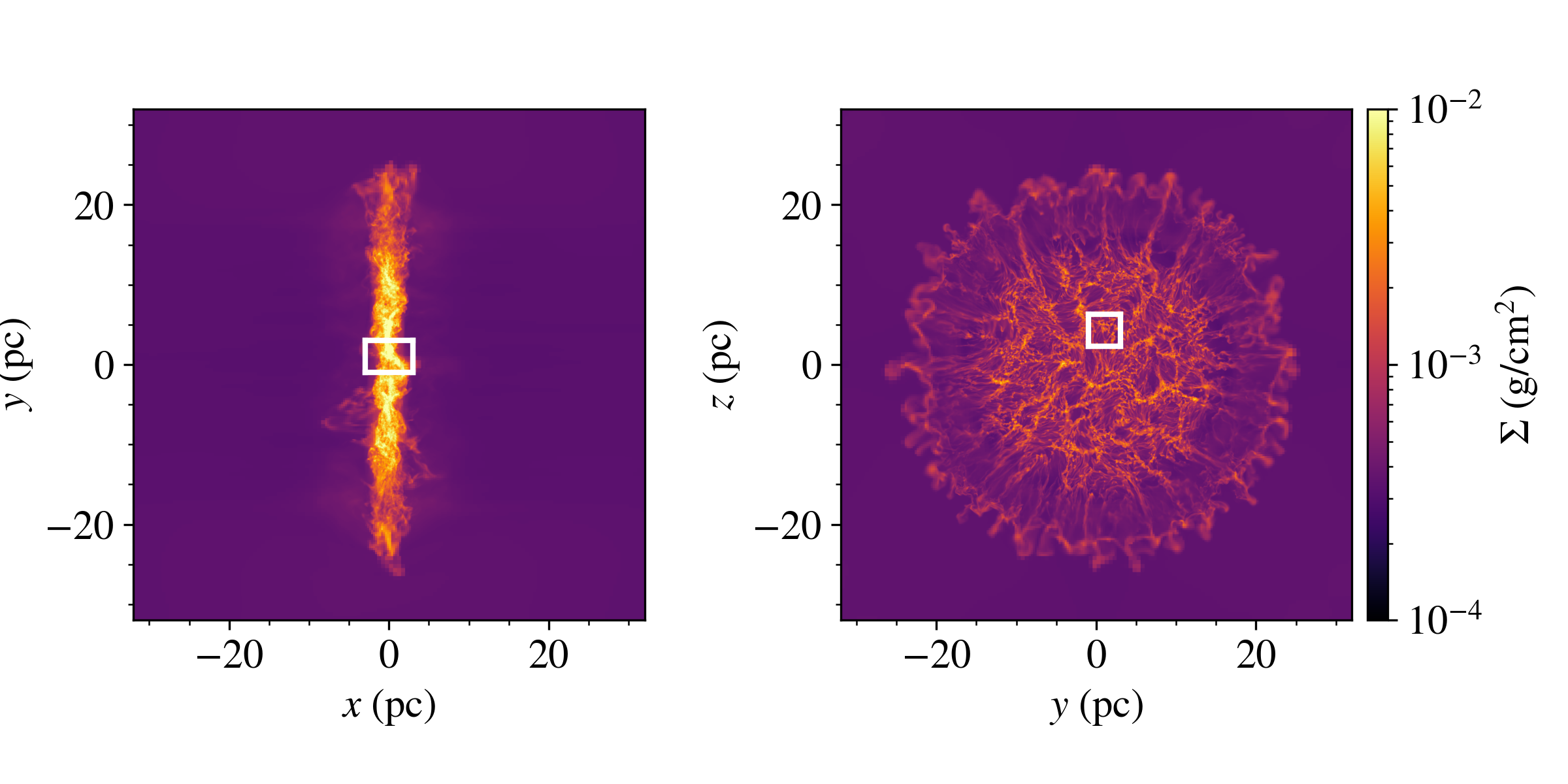
Figure 1: Column density of the cold atomic cloud’s simulation at $5\mbox{\,Myr}$. The highlighted region (R1) is examined in 3D in order to show the magnetic field and density morphology.

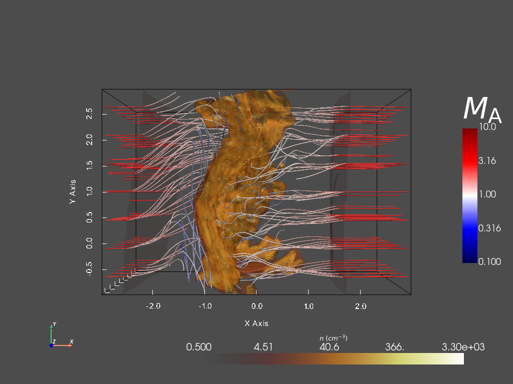
Figure 2: The density structure and magnetic field lines of the region R1 are shown after 5 Myr of evolution. The magnetic field lines are colored by the Alfvénic Mach number. Note that at this evolution time, magnetic field lines are almost perpendicular to their original orientation along the $x$ axis and the change from superalfvénic to transalfvénic of magnetic field lines across the shock. The dark-shaded regions at both sides of the center are the shock fronts where magnetic field lines start to bend. We provide an animation showing the evolution of this region as supplementary material.

3 Alignment of magnetic field lines with cold atomic clouds

To quantify the alignment of magnetic field lines, we use the histogram of relative orientations (HRO; Soler et al. 2013), which is a statistical tool to measure the angle ($\phi$) between the magnetic field and the density gradient of structures in the ISM, over number density intervals relevant to the multi-phase nature of CACs. These intervals comprise the densities of the post-shock warm neutral medium ($n\in[3,10]\ \rm{cm^{-3}}$), the low-density cold neutral gas ($n\in[10,3\times 10^{1}]\ \rm{cm^{-3}}$), the medium-density cold neutral gas ($n\in[3\times 10^{1},10^{2}]\ \rm{cm^{-3}}$), the high-density neutral gas ($n\in[10^{2},3\times 10^{2}]\ \rm{cm^{-3}}$), and the density range of the central region ($n\in[3\times 10^{2},10^{3}]\ \rm{cm^{-3}}$). We show the resulting HRO in the left panel of Figure 3 in terms of $\cos\phi$. Thus, when $\cos\phi=0$, the magnetic field is parallel to the density isocontours, while, when $\cos\phi=\pm 1$, the magnetic field is perpendicular to the density isocontours. We keep this convention to compare to the three-dimensional HRO diagram presented in Soler et al. (2013). We can see that the HRO for all density intervals peaks at $\cos(\phi)=0$; in other words, the magnetic field tends to be parallel to the density structures throughout the density range we investigate.

In order to quantify the HRO, Soler et al. (2013) introduced the shape parameter $\zeta$ defined as

$$\zeta\equiv\frac{A_{c}-A_{e}}{A_{c}+A_{e}},$$ (2)

where $A_{c}$ is the central area under the HRO diagram located between $\phi\in[75.52^{\circ},104.48^{\circ}]$, corresponding to mostly parallel magnetic field, while $A_{e}$ is the area under the HRO in the range $\phi\in[0^{\circ},41.41^{\circ}]\cup[138.59^{\circ},180^{\circ}]$, corresponding to mostly perpendicular field. Thus for a given density interval, if $0<\zeta<1$, the magnetic field lines are parallel to the density gradients, while if $-1<\zeta<0$, the magnetic field is perpendicular to the density gradients. Finally, $\zeta$ close to zero happens when there is no clear tendency in the alignment.

In the bottom panel of Figure 3, we plot $\zeta$ for the simulation in the density ranges defined above, showing that the magnetic field becomes increasingly parallel to the density gradient as the density increases up to $3\times 10^{2}\mbox{\,cm}^{-3}$, and then the degree of parallel alignment decreases for the last interval.

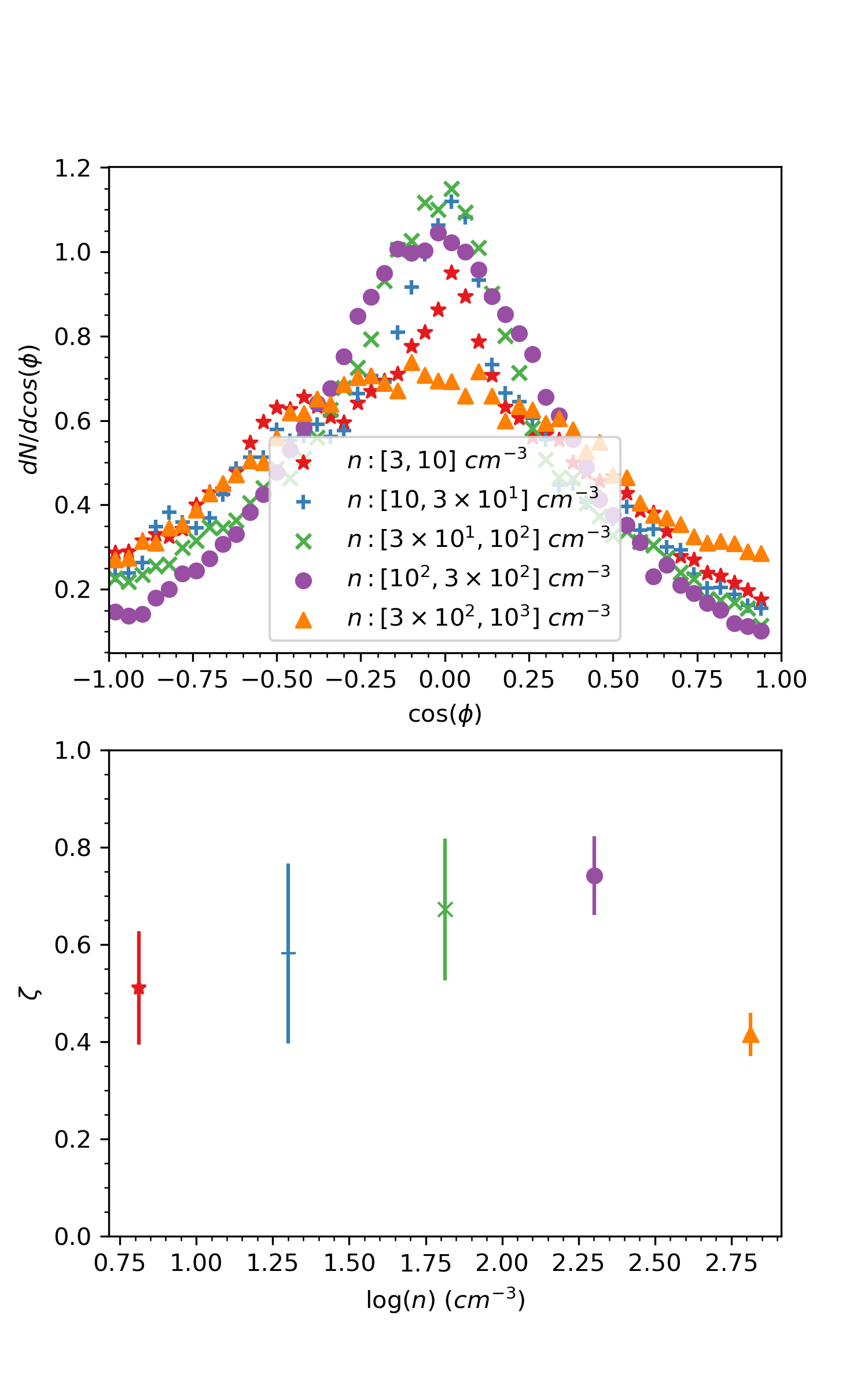
Figure 3: Top: HRO diagram for four different number density intervals. Bottom: shape parameter (see eq. 4.3) versus number density. As we can see in this figure, the magnetic field is increasingly parallel for the first three intervals, but there is a change in the trend for the last interval.

The trend of the shape parameter shown in Figure 6 of Soler et al. (2013) indicates that the alignment of the magnetic field and isodensity contours becomes less parallel as the density increases. In that work, the authors sample density values $n\in[1.6\times 10^{2},3.16\times 10^{6}]\ \mbox{\,cm}^{3}$ in isothermal simulations of cold molecular gas. In contrast, since we are interested in understanding how this correlation arises as the cloud is assembled, our simulation starts with warm atomic gas leading to density structures with $n\in[6\times 10^{-1},2.2\times 10^{3}]\ \mbox{\,cm}^{3}$. Therefore, the obtained HRO shape parameter in Figure 3 complements the one obtained by Soler et al. (2013), as it corresponds to gas that can be considered the precursor of a molecular cloud. Specifically, the HRO and shape parameter obtained in Figure 3 shows an increase in the degree of parallel alignment for the first four density intervals, while for the last one, we can appreciate a change of this tendency towards a non-preferential orientation, which corresponds to the lowest density interval in the results of Soler et al. (2013).

In Figure 4, we show the density structures between the four highest density intervals used to obtain the HRO and shape parameter of Figure 3. It can be seen from this figure that the magnetic field (black arrows) tends to be parallel to the density structures for the four density intervals. However, for the highest density interval, the magnetic field does not follow this general trend in some regions, leading to the observed change in the shape parameter.

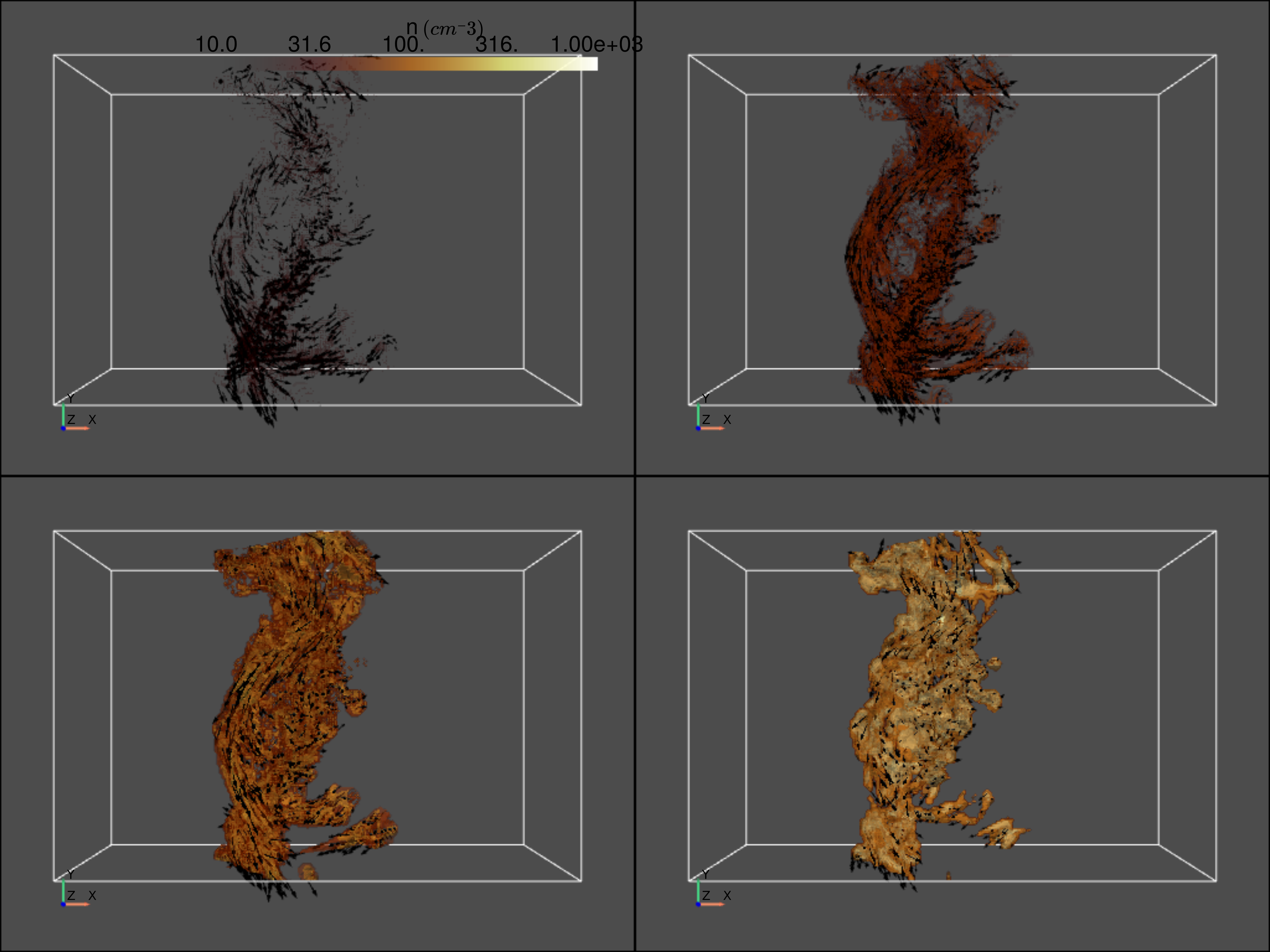
Figure 4: Regions used to compute the HRO diagram and the shape parameter shown in Figure 3. The yellow surfaces are density isocountours and the dark arrows represent the magnetic field. The top left panel corresponds to gas with density $n\in[10,30]\ \mbox{\,cm}^{-3}$, the top right panel $n\in[30,100]\ \mbox{\,cm}^{-3}$, the bottom left $n\in[100,300]\ \mbox{\,cm}^{-3}$, and the bottom right $n\in[300,1000]\ \mbox{\,cm}^{-3}$. It can be seen that, for the four density intervals shown here, the magnetic field is noticeably parallel to the density structures. However, the magnetic field shows a deviation from this trend for the highest density interval in the bottom right panel. We provide animations showing these regions as complementary material.

4 Magnetic field line evolution

To understand the alignment of the magnetic field with CACs shown in the previous section, we followed the evolution of the magnetic field lines. The resulting configuration of the three-dimensional density structures and magnetic field lines of Region R1 after 5 Myr of evolution is shown in Figure 2, where we can see the shock fronts at each side of the central condensation region. The magnetic field lines start bending at these shock fronts along their way from the center of the computational domain.

As can be seen in the provided animation (Fig. 2), the magnetic field lines change their direction from being nearly parallel to the $x$-axis at early times to being mostly perpendicular to it after $5\mbox{\,Myr}$ in the neighborhood of the dense layer. In this section, we investigate how this occurs.

4.1 Magnetic field amplification by MHD shocks

As seen in Figure 2, and considering the shock front located at the right of the condensation layer, we see that the angle between the upstream magnetic field and the normal to the shock front satisfies $\theta\approx 0$ for all the magnetic lines shown. The small variations of $\theta$ around zero are due to the fact that the shock front is not a plane when it moves away from the central region because of the fluctuations added to the inflow velocity in the simulation setup.

Following Delmont & Keppens (2011), the fast magnetosonic speed $u_{f}$ is defined as:

$$\centering u_{f}^{2}=\frac{1}{2}\left(c_{s}^{2}+u_{\rm{A}}^{2}+\sqrt{(c_{s}^{2}+u_{\rm{A}}^{2})^{2}-4u_{\rm{A,n}}^{2}c_{s}^{2}}\right),\@add@centering$$ (3)

where $u_{A}$ is the Alfvén speed and $u_{A,n}$ is its component normal to the shock front. Defining $u_{n}$ as the flow speed normal to the shock, the flow is referred to as superfast when $|u_{n}|>u_{f}$. Since $u_{A,n}\approx u_{A}$ and $u_{n}\approx u_{0}$ for the preshock flow in the three-dimensional simulation described in Section 2, it can be seen from equation (3) that this flow is superfast. The downstream flow, just after the shock front, becomes transalfvénic as we can see from Figure 2. Therefore the relation $u_{f}>|u_{n}|>u_{A,n}$, which characterizes a subfast flow, is satisfied downstream.

Such MHD shock, going from a superfast to a subfast flow, is called a fast MHD shock (Delmont & Keppens, 2011), whose main feature is that it refracts the magnetic field away from the shock normal due to the amplification of the magnetic field component parallel to the shock front. This amplification is given by

$$B_{\parallel,2}=\frac{r_{\rho}B_{\parallel,1}(M_{A,1}^{2}-\cos^{2}\theta)}{M_{A,1}^{2}-r_{\rho}\cos^{2}\theta},$$ (4)

where $B_{\parallel,1}=B_{1}\sin\theta$ and $B_{\parallel,2}$ are the upstream and downstream magnetic field components parallel to the shock front, $r_{\rho}=\rho_{2}/\rho_{1}$ is the ratio of the downstream ($\rho_{2}$) and upstream ($\rho_{1}$) densities, $M_{A,1}$ is the Alfvénic Mach number of the upstream gas, and $\theta$ is the angle between the vector normal to the front-shock and the upstream magnetic field $\bm{B}_{1}$. Since this amplification depends on the angle $\theta$, the fluctuating curvature of the shock front at different positions yields the inhomogeneous downstream magnetic field pattern when the shock front travels away from the central region, early in the evolution times (see Figure 2).

4.2 Line bending analysis

To understand how magnetic field lines change their original direction in the post-shock region, we consider the induction equation in ideal MHD,

$$\frac{\partial\bm{B}}{\partial t}=-\bm{B}\nabla\cdot\bm{u}-(\bm{u}\cdot\nabla)\bm{B}+(\bm{B}\cdot\nabla)\bm{u}.$$ (5)

4.2.1 Line bending by a compressive flow

This analysis takes place after the magnetic field component parallel to the shock front is amplified by the fast MHD shock, i.e., in a region containing cooling and thermally unstable gas. After the amplification, magnetic field lines adopt the shape represented in Figure 5, where the magnetic field component parallel to the shock front, $B_{y}$, has been amplified, and the magnetic field component perpendicular to the shock front $B_{x}$ stays constant, in agreement with the jump condition for the magnetic field.

Furthermore, we assume that the flow speed decreases along $x$ in the post-shock region; i.e., $u_{x}=u_{x}(x)$ and $\partial u_{x}/\partial x<0$, which represents the compression caused by the cooling of the gas as it travels downstream. Finally, we disregard the downstream component of the velocity parallel to the shock front, $u_{y}$ and $u_{z}$, to analyze the effect of the compression alone.

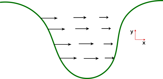
Figure 5: Initial line bending model. The magnetic field is represented by the green line, while the velocity field is represented by the black arrows.

To validate these assumptions, in Figure 6 we plot the relevant physical quantities at time $t=0.7\mbox{\,Myr}$ along a ray parallel to the $x$ axis passing through a region in which this amplification becomes large at later evolutionary times. In the top panel, the shock front and condensed region are clearly visible in the gas density profile. The middle panel shows that, in addition to the discontinuity at the shocks, the inflow velocity $u_{x}$ smoothly decreases downstream from the shock, in sync with the density increase. Also, $u_{y},\ u_{z}\approx 0$, in agreement with our assumptions. Finally, in the bottom panel, we see that the fluctuation of $B_{x}$ remains within $\lesssim 20\%$ of its mean value, so it is negligible to the first order.

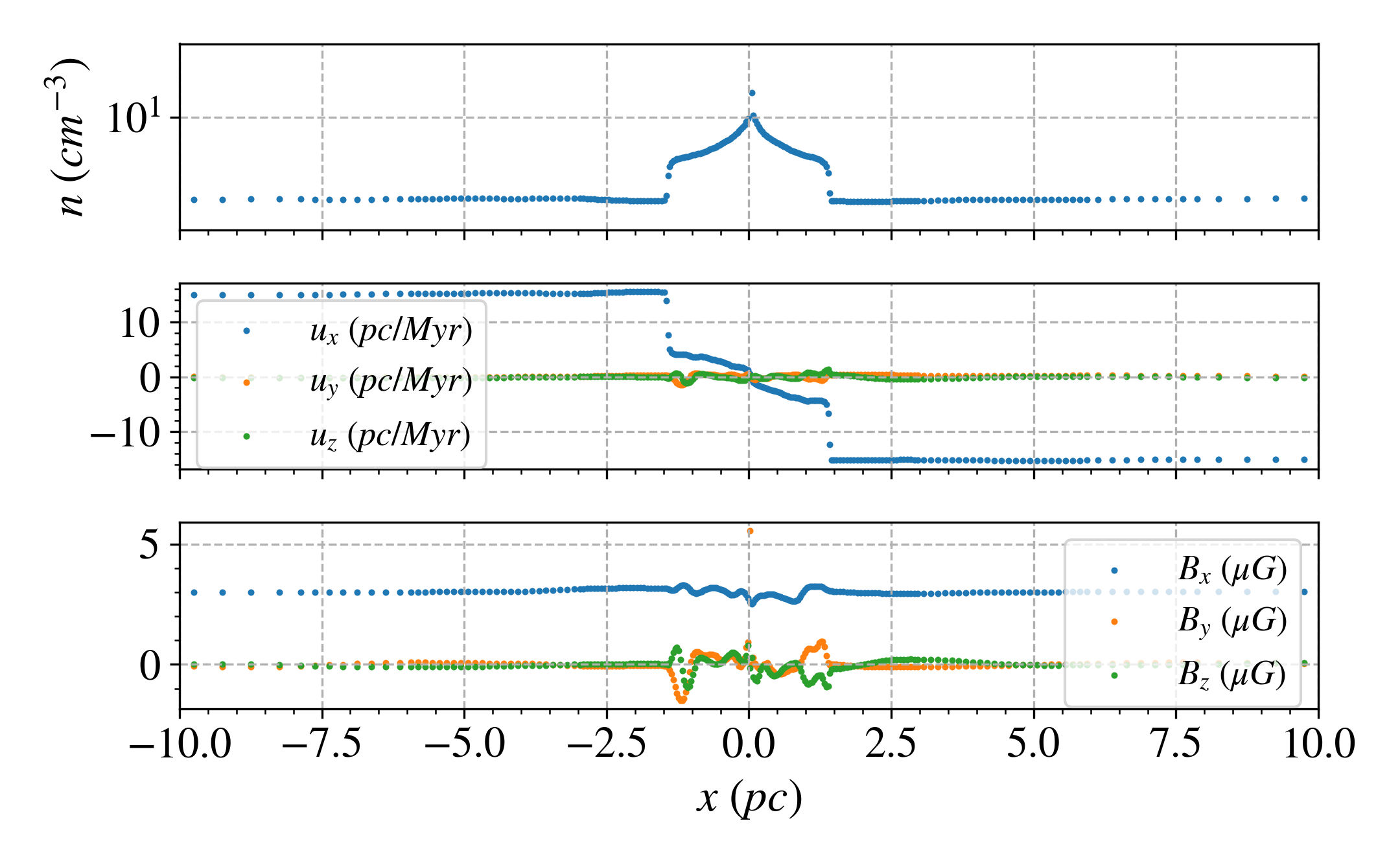
Figure 6: Number density (top), velocities (middle), and magnetic fields components (bottom) along a ray parallel to the $x$ axis at time $t=0.7$ Myr. It can be seen that the profile of these quantities agrees with the assumptions made for the line bending analysis.

Therefore, the assumptions $B_{y}=B_{y}(x)$, $B_{x}=C$, where $C$ is a constant, $u_{x}=u_{x}(x)$, with $\partial u_{x}/\partial x<0$, $u_{y},u_{z}\rightarrow 0$, and solving for the $B_{y}$ component, reduce equation (5) to

$$\centering\frac{\partial B_{y}}{\partial t}=-B_{y}\frac{\partial u_{x}}{\partial x}-u_{x}\frac{\partial B_{y}}{\partial x}.\@add@centering$$ (6)

This equation can also be written in Lagrangian form as

$$\centering\frac{dB_{y}}{dt}=-B_{y}\frac{\partial u_{x}}{\partial x}.\@add@centering$$ (7)

Thus, since $\partial u_{x}/\partial x<0$, eq. (7) implies that $dB_{y}/dt$ has the same sign as $B_{y}$, and therefore the magnetic field component $B_{y}$ is always amplified by the downstream compressive velocity gradient. This amplification results in the magnetic field aligning to the condensation plane where CACs form.

4.2.2 Line bending at curved interfaces

Another possible mechanism for aligning the magnetic field with the density structures occurs when the collision interface is curved rather than flat, as, for example, in the case of the NTSI (Vishniac, 1994). To investigate this, we also ran two-dimensional simulations with the same initial conditions and physics as the three-dimensional simulation described in Section 2 but with a curved collision interface, obtained by adding a sinusoidal displacement perturbation (a “bending mode” perturbation). In the left panel of Figure 7, we show a very early stage of this simulation. In this case, the obliqueness of the interface implies the existence of a component of the incoming flow tangential to it, while the perpendicular component is reduced across the shock. This causes the flow to change direction at the interface, being now oblique to the original magnetic field direction. Being transalfvénic, this oblique post-shock flow can begin bending the field lines. The situation is symmetric on both sides of the layer, thus generating a shearing velocity field with opposite directions at opposite sides due to the different concavity of the collision interface. This generates an “S” shape of the magnetic field lines across the shocked layer. A later stage of this simulation is shown in the right panel of Figure 7, showing that the flow tends to be subalfvénic in the condensed regions.

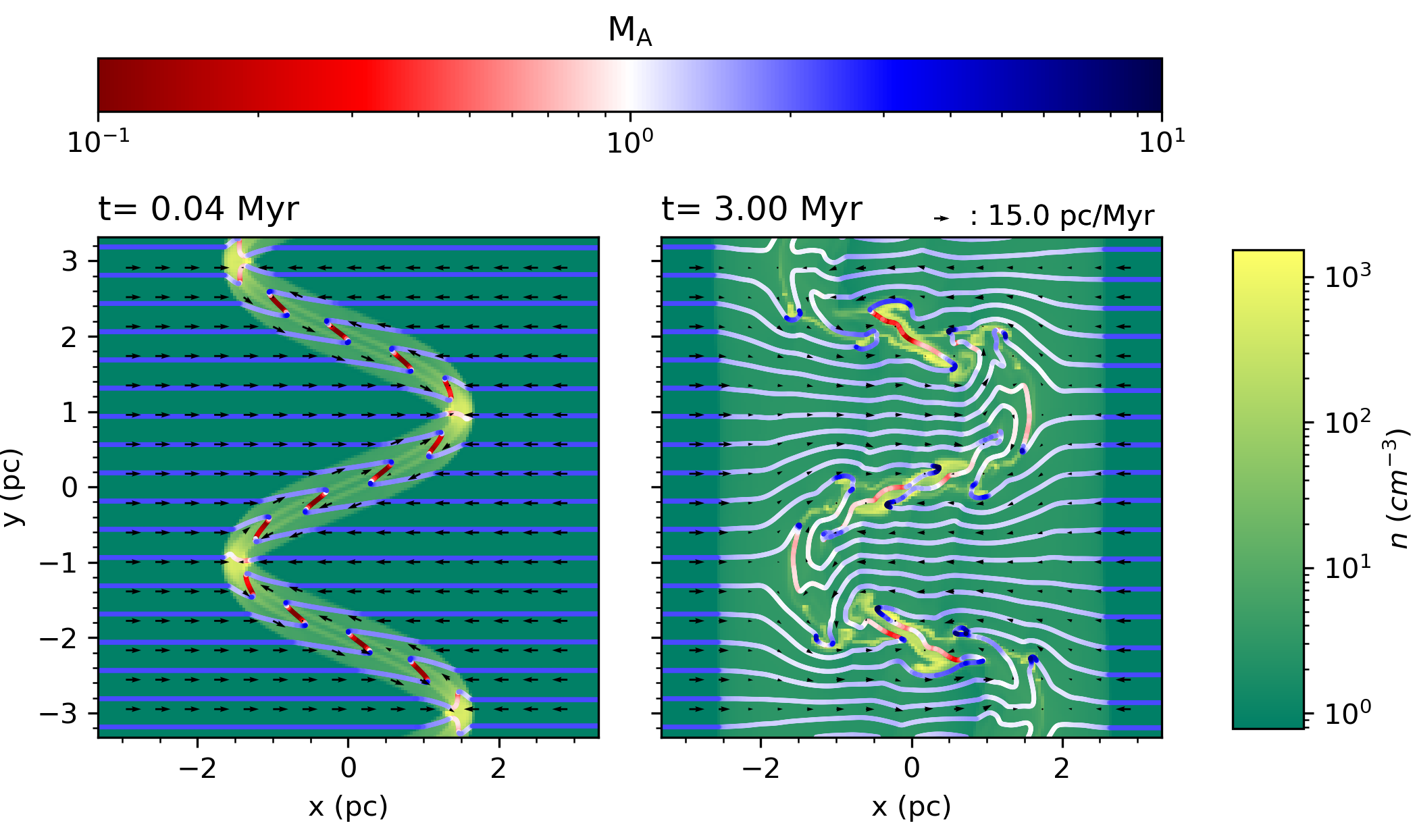
Figure 7: Two-dimensional simulation of warn atomic colliding flows with a curvilinear collision interface at 0.04 Myr (left panel) and 3.0 Myr (right panel). The two color bars represent the number density and the Alfvénic Mach number.

For this collision interface, the line-bending analysis differs from that described in Section 4.2. In this case, we will have a velocity field like the one represented in Figure 8, where the left panel represents an unperturbed downstream magnetic field line and the right panel represents a perturbed one. In the left panel, we consider a local system of coordinates centered at the point where the $u_{y}$ is maximum. The magnetic field line is represented in green, the $x$-axis is parallel to the field line, the $y$-axis is perpendicular to it, and the velocity field is represented by black arrows.

Figure 8: Line bending model for the colliding flows with curvilinear collision interface. The left panel represents the initial state and the right one the evolution according to the analytical model given by equation (8). In this sketch, the black arrows are the velocity field.

Thus, initially, $B_{y}=0$ and $B_{x}=C$, where $C$ is a constant. Then, considering $u_{x}$, $u_{z}\rightarrow 0$, and $u_{y}=u_{y}(x)$, we obtain, from equation (5),

$$\frac{\partial{B_{y}}}{\partial t}=B_{x}\frac{\partial u_{y}}{\partial x}.$$ (8)

We can then consider the previous equation in three different regions in the left panel of Fig. 8: First, in the region $x\in[x_{1},0]$, we have $\partial u_{y}/\partial x\ >\ 0$, and so $\partial B_{y}/\partial t\ >\ 0$. Second, in the region $x\in[0,x_{2}]$, we see that $\partial u_{y}/\partial x\ <\ 0$, and therefore $\partial B_{y}/\partial t\ <\ 0$. Finally, in the region $x\in[x_{2},x_{3}]$, $\partial u_{y}/\partial x\ >\ 0$, thus $\partial B_{y}/\partial t\ >\ 0$.

Therefore, for these three regions, the sign of $\partial B_{y}/\partial t$ explains the deformation of the magnetic field line having an ”S” shape morphology where each convex part aligns the direction of the flow (See Figures 7 (left panel) and 8).

5 Discussion

5.1 The role of the pre-condensation shock in the alignment of the magnetic field

As we have seen from the three-dimensional simulation, magnetic field lines change their orientation at the shock front due to the effect of the fast MHD shock. The passage of the shock front yields an irregular amplification of the parallel component to it, which results in the early downstream shocked magnetic field line pattern. Afterward, magnetic field lines are dragged and folded by the downstream decelerating gas.

In this work, we do not vary the relative orientation between the upstream magnetic field and the shock front of the system in the initial condition. However, there is a small range of angles between them due to the departure of the shock front from a perfectly flat plane due to the velocity fluctuations. The influence of the initial angle between the magnetic field and the shock front has been studied in Inoue & Inutsuka (2016), who found that the number of CACs or fibers oriented perpendicular to the magnetic field increases with the orientation angle of the upstream magnetic field and the shock front for simulations without an initial velocity dispersion. However, when an initial velocity dispersion is included, the authors find that fibers tend to be oriented in the direction of the local magnetic field. For this reason, they conclude that the formation mechanism of fibers and their alignment with the local magnetic field is the turbulent shear strain, which was also identified as the reason for the elongation of filamentary CACs by Hennebelle (2013).

It is important to mention that the role of MHD shocks in the evolution of magnetic field lines that yield the final correlation has not been explored before. In this work, we identified that a fast MHD shock produces magnetic field fluctuations that get amplified between the shock front and condensation layer.

5.2 The role of the velocity gradient in aligning the field and density structures. The case of gravitationally-driven cloud formation

Soler & Hennebelle (2017) proposed that the relative orientations between the magnetic field and density structures $\phi=90^{\circ}$ and $\phi=0^{\circ}$ might be equilibrium points. However, the reason for that is unknown. In this work, we identified that it is the action of a fast MHD shock and the compressive velocity resulting from the gas settlement onto the dense layer that leads to $\phi=90^{\circ}$.

Since we have focused on non-gravitational CACs, we have not numerically explored how $\phi$ becomes $0^{\circ}$. However, a discussion similar to that in Section 4.2.1 leads us to speculate that the $\phi=0^{\circ}$ configuration may arise in the presence of a stretching velocity field, as it would be the case of the tidal flow into the gravitational well of a strongly self-gravitating cloud. In this case, $x$ would be the direction of the flow and $B_{y}$ is a magnetic field perturbation perpendicular to that direction. Therefore, equation (7) for a positive velocity gradient implies that $dB_{y}/dt$ has the opposite sign to $B_{y}$, straightening the field lines. Thus, we suggest that the induction equation in the presence of a compressive or stretching velocity field leads to the $\phi=0,90^{\circ}$ equilibrium configurations found by Soler & Hennebelle (2017), justifying their speculation that they may be attractors. This also suggests a mechanism for the parallel alignment of the magnetic field to non-self-gravitating structures and its perpendicular alignment to self-gravitating ones, as observed in Gómez et al. (2018).

5.3 The effect of strong cooling on the development of the NTSI

Regarding the development of the NTSI, Vishniac (1994) found that the requirement for this instability to grow is that the displacement of the cold slab is larger than its thickness. This condition can only be satisfied when there is a high compression ratio across the shock yielding a very thin shocked layer. In the isothermal case, this requires that $M_{\rm s}^{2}\gg 1$. The three-dimensional simulation described in Section 2 has $M^{2}_{\rm s}=4.0$, which is not too large. However, our simulations include strong cooling leading to thermal instability, which produces a much stronger compression of the condensed layer and a much thinner slab dimension, even for moderate Mach numbers (Vázquez-Semadeni et al., 1996). So, it is not difficult to fulfill the requirement for the development of the NTSI at the condensed, rather than the shocked, layer (Hueckstaedt, 2003), as demonstrated by the growth of the bending mode perturbation (the increase in the curvature) for the dense layer in our 2D simulation. This means that NTSI can be triggered by not-so-strong shocks in the strongly cooling case.

5.4 The effect of the magnetic field on the NTSI and the shear strain

The NTSI is one of the possible mechanisms yielding the shear strain proposed by Hennebelle (2013) to be responsible for the elongation of filamentary CACs and the alignment of these structures with the local magnetic field, since it produces the momentum transport from the original inflow direction to that parallel to the dense layer in the regions around the nodes, as can be seen in Figure 7. However, Heitsch et al. (2007) found that when the magnetic field is aligned with the inflow, it tends to weaken or even suppress the NTSI due to the magnetic tension counteracting the transverse momentum transport. Nevertheless, the NTSI can contribute to the change of direction of the magnetic field if the flow surrounding the dense layer, remains at least transalfvénic, so that it has sufficient energy to bend the field. This condition is indeed satisfied by the flow between the shock and the condensation front, as can be seen for the 2D simulation in both panels of Figure 7. Note, incidentally, that the flow inside the dense layer is generally subalfvénic.

Another source of shear strain that does not require the NTSI is observed in our 3D simulation, which does not include an initial bending-mode perturbation to the locus of the collision front. This arises later in the evolution, when the magnetic field lines have already been dragged and bent by the compressive velocity field. At this time, the transalfvénic condition of the post-shock flow allows the magnetic field to partially re-orient the gas flow along them. Since the field lines have been oriented nearly parallel to the dense layer by the compressive post-shock flow, the velocity field is also oriented in a similar way, and in opposite directions on each side of the dense layer, therefore adding a strong shear component to the flow around the layer. We can see one example of this situation in Figure 9, where the velocity fields are represented by dark arrows and the magnetic field lines are color-coded with the Alfvénic Mach number. In this Figure, the troughs and peaks of the CACs do not show corresponding converging and diverging velocity fields, as would correspond to the NTSI, and so the structure at this point appears not have been formed by this instability.

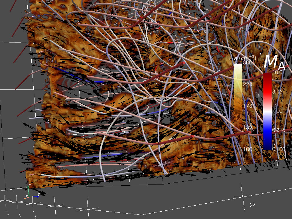
Figure 9: A couple of filamentary CACs located in the left-down corner. In the provided animation showing this region, it can be seen a turbulent shear strain velocity field along their main axis and aligned with the local magnetic field. Note that the velocity field on the filamentary CACs is different from the one expected in the case of the NTSI.

5.5 Inhibition of turbulence generation by the magnetic field

It has been noticed in previous works that MHD simulations of cloud formation are less turbulent and show more filamentary structure than pure hydrodynamical simulations (e.g., Heitsch et al., 2007, 2009; Hennebelle, 2013; Zamora-Avilés et al., 2018). The generation of turbulence in curved compressed layers is due to the KH instability, which in turn is triggered by the shear flow produced by the NTSI (e.g. Blondin & Marks, 1996; Heitsch et al., 2006). Therefore, the magnetic tension, which opposes the vorticity generation by the shear flow across the dense layer, may suppress the development of the KHI and, as a consequence, the generation of turbulence. Indeed, a 2D numerical simulation without the magnetic field exhibits a much stronger turbulence level, as shown in Fig. 10.

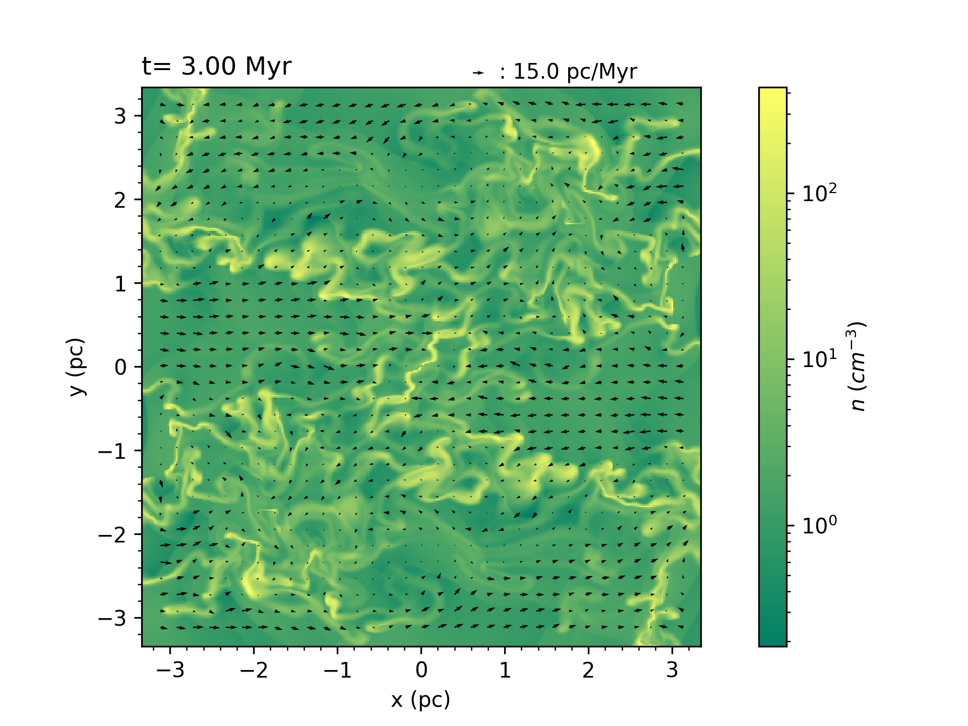
Figure 10: Non-magnetic version of the two-dimensional simulation shown in Figure 7.

5.6 Comparison with previous work

The superalfvénic nature of the initial inflow in our simulations, and its continuation downstream as a transalfvénic flow, allow the dragging and amplification of the magnetic field, in agreement with Skalidis et al. (2022) whose observations reported transalfvénic turbulence in the Hi-H₂ transition region. According to these authors, atomic gas might accumulate along magnetic field lines, which is also in agreement with our results (see Figure 9).

In this work, our simulations consider only the formation of clouds by the collision of converging cold atomic flows. However, the main physical processes responsible for the alignment of magnetic field lines and density structures, MHD shocks, and the NTSI, can be also present at the interfaces between interacting wind-blown bubbles and/or supernova shells. Therefore, the MHD shocks and the NTSI could also be the principal physical mechanisms behind the magnetic field alignment with fibers found in this type of object by Clark et al. (2014).

6 Summary and Conclusions

In this work, we have studied the physical mechanisms responsible for the observed alignment of magnetic field and cold atomic gravitationally unbound density structures formed by the collision of converging warm atomic gas. We have tracked the evolution of magnetic field lines in a three-dimensional simulation having typical conditions of the warm ISM and found that they become perpendicular to their original orientation and end up aligned with density structures.

The process of the alignment of magnetic field lines with the density structures starts at the shock fronts and takes place in the cooling, thermally unstable gas, so that the magnetic field already shows a preferred orientation when the flow forms CACs at the condensed layer.

At the position of the shocks, the magnetic field changes its direction due to the amplification of its component parallel to the front, which is produced by the velocity fluctuations in the pre-shock region. This amplification occurs due to a fast MHD shock that occurs when the upstream and downstream flows are super– and sub-fast, respectively.

Behind the shock front, the compressive downstream velocity field further amplifies the magnetic field component parallel to the shock front, increasing the curvature of the lines in this region, and causing them to become increasingly parallel to the condensed layer produced by the thermal instability. The amplification of the fluctuation by a compressive velocity gradient can be understood through an analysis of the induction equation for planar geometry (eq. [7]), which shows that the change in the fluctuating field component has the same sign as the fluctuation, amplifying it.

From the same equation, we concluded that a stretching velocity gradient causes damping of the fluctuating component, leading to a straightening of the field lines, thus orienting them perpendicular to the density structures. We speculate that this is the mechanism occurring during the growth of self-gravitating structures, where the flow accelerates inwards, thus producing a tidal stretching velocity pattern, thus being a possible explanation for the perpendicular orientation of the field lines around self-gravitating molecular cloud filaments.

In conclusion, we have found that a settling (i.e., decelerating) flow, such as that occurring due to the condensation of the gas by thermal instability orients the lines parallel to the density structures, while a stretching (accelerating) one, such as infall into a potential well, orients the field lines perpendicular to the density structures. This may be the physical mechanism behind the stationarity of these configurations found by Soler & Hennebelle (2017).

Finally, we also found that, under typical conditions of the ISM, the flow upstream from the shock front is superalfvénic and becomes transalfvénic downstream. This allows the velocity field to bend and drag the magnetic field lines.