s g \NewDocumentCommand\bbos s g \NewDocumentCommand\alp s g \NewDocumentCommand\bet s g
Quantitative description of long-range order in the anisotropic spin-1/2 Heisenberg antiferromagnet on the square lattice
Abstract
The quantitative description of long-range order remains a challenge in quantum many-body physics. We provide zero-temperature results from two complementary methods for the ground-state energy per site, the sublattice magnetization, the spin gap, and the transverse spin correlation length for the spin-1/2 anisotropic quantum Heisenberg antiferromagnet on the square lattice. On the one hand, we use exact, large-scale quantum Monte Carlo (QMC) simulations. On the other hand, we use the semi-analytic approach based on continuous similarity transformations in terms of elementary magnon excitations. Our findings confirm the applicability and quantitative validity of both approaches along the full parameter axis from the Ising point to the symmetry-restoring phase transition at the Heisenberg point and further provide quantitative reference results in the thermodynamic limit. In addition, we analytically derive the relation between the dispersion and the correlation length at zero temperature in arbitrary dimension, and discuss improved second-moment QMC estimators.
I Introduction
The collective behavior of matter is one of the most important topics of modern science. Understanding it is crucial in basic research as it holds the key to a variety of correlated many-body states - realized for example in topologically ordered quantum phases such as spin liquids and fractional quantum Hall liquids or superconductors. At the same time, it is clear that this understanding forms the basis for many technological applications such as magnetic data storage [1] and spintronics [2, 3] which define the modern era. In particular, it is decisive to gain a systematic and quantitative understanding of collective phenomena.
Quantum magnetism has turned out to serve as a very fruitful playground to study collective quantum phenomena. Indeed, frustrated magnets are known to host a variety of exotic quantum phases such as spin-liquid ground states with topological quantum order. Unfrustrated quantum antiferromagnets with long-range magnetic Néel order play an important role for the physics of the high-temperature superconductors [4], because the undoped parent compounds represent two-dimensional antiferromagnetic Heisenberg magnets with on the square lattice [5]. Furthermore, spintronics is a huge field of applications in which the manipulation of magnetism is crucial [1, 3, 2] requiring a fundamental understanding of the underlying mechanisms.
It is very common to describe the magnetic excitations of quantum antiferromagnets by essentially interaction-free magnons [6]. By “essentially free of interactions” we mean that some static renormalization of the dispersions is accounted for, but the magnon-magnon scattering processes are rarely considered quantitatively. Yet it turned out that the interaction of the magnons is very important to understand certain dips (dubbed ‘roton dips’) in the dispersion [7, 8] and the distribution of spectral weight in the continua [9]. This has been shown by establishing a continuous basis change, namely a continuous similarity transformation (CST), such that the number of magnons in the target basis is conserved, at least to very good approximation [7, 9, 10]. This facilitates the interpretation of the results greatly, for instance the dispersion can be read off immediately. Continua at zero temperature formed from two or three elementary excitations [11] only require to solve a two- or three-particle problem avoiding complicated diagrammatic techniques. In this fashion, also bound states of two [12, 13, 14, 15] or three particles [11] were identified.
To support these calculations and to assess their validity, we turn to static quantities such as the ground-state energy per site , the sublattice magnetization , the spin gap , and the transverse spin correlation length and compare theoretical results for them stemming from two very different approaches.
One is the above-mentioned CST which maps the original model expressed by magnon creation and annihilation operators to an effective model in magnon operators, but with conservation of the number of magnons. The CST consists in setting up a general flow equation in all couplings and solving this flow equation. The first step is analytical, the second numerical eventually providing the coupling constants of a magnonic model in second quantization. Thus, we classify this approach as semi-analytical.
The second approach are quantum Monte Carlo (QMC) simulations using the stochastic series expansion (SSE) algorithm with directed-loops [16, 17, 18, 19], which is a well established numerically exact method for unbiased, large-scale studies of quantum magnets.
Our work demonstrates the applicability and quantitative validity of CST and QMC along the full parameter line from the Ising to the Heisenberg model. In particular, we capture the phase transition from the gapped ordered phase at any finite anisotropy to the gapless Heisenberg point with full SU(2) symmetry. Our results confirm that associated critical exponents at this symmetry-restoring phase transition are given exactly by the ones from spin-wave theory.
The article is set up as follows. In the following section II we briefly introduce the model and describe the two employed complementary methods concisely with an emphasis on how the particular quantities are computed. The results are presented and discussed in Sect. III. The summary IV concludes the article.
II Model and Methods
II.1 Model
We consider a Heisenberg quantum antiferromagnet with and easy-axis anisotropy defined by the anisotropy parameter so that the Hamiltonian takes the form
| (1) |
in terms of the spin ladder operators. The model is bipartite and thus unfrustrated. It breaks the symmetry of spin flips by displaying long-range alternating magnetic order with a finite sublattice magnetization at zero temperature. We assume to be positive for simplicity, but its negative value is physically equivalent. At the spin isotropic point the continuous SU(2) symmetry is restored so that the elementary excitations, the magnons, become Goldstone bosons with vanishing spin gap [6]. For any value a finite energy gap is present, which takes the value in the Ising limit . No rigorously exact results are known for this model for . But there is a wealth of evidence for its characteristic behavior [5, 6, 20]. Since the singular behaviour at the Heisenberg point originate from Goldstone excitations and not by critical fluctuations, the associated exponents are expected to correspond exactly to the spin-wave values [21]. This has been confirmed by high-order series expansions about the Ising limit as well as CST for the closing of the one-magnon gap [21, 22, 10] with an exponent .
II.2 Methods
Next, we briefly sketch the two approaches used.
II.2.1 Quantum Monte Carlo simulations
The starting point of the SSE QMC method is a high-temperature expansion of the quantum partition function
| (2) |
Here, denotes an orthonormal basis of the full Hilbert space and the expansion order of the exponential term. Further, is decomposed into a sum of local bond operators , characterized by a bond and an operator type . These bond operators are chosen such that, given the basis , they are non-branching, i.e. . The standard approach for the basis, which we also use here, is a product state of local eigenstates, i.e. . Here, a suitable bond decomposition is given by the operators
| (3) |
that are diagonal in as well as the offdiagonal bond operators
| (4) |
The different products of bond operators contributing to can be encoded into an ordered operator sequence , thus yielding for the quantum partition function
| (5) |
The length of corresponds to the expansion order and thus fluctuates. For numerical simulations, however, it is more convenient to truncate the sum to a maximal expansion order . Since the average expansion order is (sharply) centered around , this cutoff does not introduce any systematic error in practice as long as we always ensure . A fixed length operator string can be obtained by padding with unity operators , which finally yields for the quantum partition function
| (6) |
where an additional combinatorial factor has to be introduced to account for the possible insertion positions of the unity operators. Here, the expansion order corresponds to the number of non-unity operators in . For a bipartitite lattice, such as the square lattice considered here, all finite contributions to in Eq. 6 can be rendered positive, upon adding an appropriate constant to the diagonal [16]. To efficiently sample the configuration space by means of Markov Chain Monte Carlo, a tandem of two updates is usually carried out. In a first local update step [16, 17], diagonal operators are inserted or removed in , effectively sampling the expansion order . The next update is the directed-loop update [18, 19]. Here, by carrying out a succession of local bond operator updates, a global and efficient update to sample different operator types, i.e. both diagonal and offdiagonal, in as well as is obtained. For more details we refer the reader to Refs. [18, 23].
When approaching the Ising limit , we would ideally like our updating procedure to reduce to a classical (cluster) update on the spins in . While this is indeed the case for the word-line based loop algorithm (cf. Ref. [24] for a review), which reduces in the Ising limit to a classical Swendsen-Wang cluster update [25] for [26], this is not the case for the directed-loop update in the SSE picture for the following reasons. Flipping a spin in here corresponds to flipping the spin on all operators in that are connected to that site. For the local bond operator updates during the directed-loop update, there is in the general case always the possibility to backtrack the loop propagation (this is also referred to as a “bounce”). As the probability for these bounces becomes large for , this process becomes very inefficient for , since the number of operators connected to a site is proportional to [18]. A simple trick to overcome this issue is to perform a unitary rotation in spin space, resulting in the Hamiltonian
| (7) |
Rotating the Hamiltonian in spin space such that the largest matrix elements are associated with off-diagonal bond operators more generally seems to help with sampling issues that arise in the directed-loop update, as recently reported in spin-1 systems with single-ion anisotropies [27] or in spin-1/2 models [28].
Thus, we always carry out simulations for the rotated Hamiltonian . In the following, we briefly discuss how we measure the relevant observables, where () refers to thermal expectations with respect to (). We further note, that we always simulate quadratic lattice geometries with sites and periodic boundary conditions.
In terms of the SSE, the energy is related to the average expansion order and given by . To obtain an estimate of the ground-state energy per spin in the thermodynamic limit, we simulate for linear system lengths at inverse temperature and linearly extrapolate the data, using the leading finite size behavior .
While the spectrum of the Hamiltonian is not directly accessible within the SSE approach, it is indirectly encoded in imaginary time correlation functions
| (8) |
where is some operator and denotes the imaginary time. If is chosen such that it excites the ground state, i.e. and , the ground-state excitation gap can be efficiently estimated in the thermodynamic limit (TDL) based on a (convergent) sequence of moments of as introduced in Ref. [29]. Here an order gap estimator is constructed using the Fourier components of
| (9) |
where denote bosonic Matsubara frequencies. The gap estimator is then given as follows
| (10) |
where the numbers are defined by . Here, the important property
| (11) |
holds, where the limits are in particular interchangeable. For more details we refer the reader to Ref. [29]. A suitable operator for the one-magnon excitations is the staggered magnetization in the spin- direction such that we consider . For the gap estimator , we measure with respect to the rotated system . In practice, as outlined in Ref. [29], a sufficient choice for convergence of is given by and , where is an initial guess of , for which we use the CST results. To eliminate finite-size effects, we choose linear system lengths of , including system lengths up to near the isotropic Heisenberg point.
The staggered longitudinal magnetization can be obtained as from the spin-spin correlation function at maximal distance [30, 31, 23],
| (12) |
where and the factor is included for to account for the SU(2) symmetry. The offdiagonal spin-spin correlation function can be efficiently measured during the directed-loop update [32, 19]. To obtain an estimate of the ground-state magnetization , we extrapolate data for linear system sizes at inverse temperatures to the TDL using the leading finite-size scaling behavior (here it is important to take the square root after the extrapolation). Close to the isotropic Heisenberg point, the finite-size effects are stronger, and we here linearly extrapolate data for linear system sizes at inverse temperatures .
The transverse correlation length quantifies the exponential asymptotic decay of the spin-spin correlation function . It is always finite for and relates to the quantum fluctuations that arise for . In addition to the dominant exponential term an algebraic factor appears for the two-dimensional system considered here. In App. A, we provide a general derivation of the algebraic correction factor within a saddle point approximation for general dimensions, and identify its actual presence explicitly for the system under consideration from QMC simulations in Sec. III. One possible means of extracting the correlation length is thus to perform a fit of the numerical data to this asymptotic decay within appropriate ranges of the distance . Another standard approach to estimate is by means of the staggered spin structure factor , defined by
| (13) |
where for the staggering sign “+1” is chosen if the sites and belong to the same sublattice and “-1” otherwise. In terms of this quantity, can be estimated by the second-moment estimator
| (14) |
where corresponds to the antiferromagnetic ordering and is one of the reciprocal lattice vectors closest to . The factor is specific to the algebraic correction term in the spin-spin correlation function, cf. App. B for other cases. For our analysis, we focus on the regime , where efficient simulations can be carried out without performing the spin rotation. To obtain better statistics, we thus measure during the directed-loop update. Further, we extrapolate the data to the TDL using polynomials of degree 3 in for linear system sizes up to and at inverse temperature .
II.2.2 Continuous Similarity Transformations
For the semi-analytic CST approach we rewrite the spin model (1) in terms of bosons according to Dyson and Maleev [33, 34] which hides the manifest hermiticity of the Hamiltonian. But it ensures that the bosonic Hamiltonian
| (15) | ||||
comprises at maximum quartic terms in the bosonic creation and annihilation operators. Here the sum runs over the sites of the sublattice where the bosons are located. The bosons are located on the sublattice while the link nearest neighbors, i.e., a site on to one of its adjacent sites on .
The next step is to Fourier transform the bosonic operators to and and their hermitian conjugates, which yields the Hamilton operator with bilinear and quartic bosonic terms in reciprocal space with wave vectors . These wave vectors are chosen from the magnetic Brillouin zone because we distinguish between both sublattices. Subsequently, we perform a standard Bogoliubov transformation to operators and to eliminate the bilinear terms creating or annihilating pairs of bosons. This is done self-consistently, i.e., the bilinear terms changing the number of bosons vanish after normal-ordering all quartic terms. Normal-ordering is meant here relative to the bosonic vacuum after the Bogoliubov transformation: all creation operators are commuted to the left, all annihilation operators to the right. Truncating the resulting Hamiltonian at the bilinear level provides the usual mean-field Hamiltonian which neglects all interactions between the elementary excitations, but comprises a static renormalization of the dispersion on the level of a self-consistent Hartree-Fock theory.
We proceed by keeping all quartic terms which generally consist of three classes of terms: (i) leaving the number of bosons invariant, (ii) changing this number by , and (iii) changing this number by . Class (i) consists of terms with two creation and two annihilation operators, class (ii) consists of terms with three creation and one annihilation operator or vice-versa. Finally, class (iii) consists of terms with four creation operators or four annihilation operators.
This quartic Hamiltonian is not manifestly hermitian because of the properties of the Dyson-Maleev representation. Thus, we apply a CST to it which is not manifestly unitary. The flow of coupling constants results from
| (16) |
where is the continuous flow parameter running from where equals the initial Hamiltonian to where one obtains an effective Hamiltonian [35, 36]. The initial Hamiltonian results from the self-consistently determined Bogoliubov transformation while the final effective Hamiltonian does no longer contain terms of classes (ii) and class (iii). In order to reach this nice property, which facilitates the subsequent interpretation, we choose the particle conserving generator [37, 38] which comprises all terms in the Hamiltonian at of classes (ii) and (iii). Those terms which increase the number of bosons have exactly the same prefactor as in while those terms which decrease the number of bosons have the opposite sign in the prefactor of the same term in .
Assuming convergence of the flow implies so that conserves the number of excitations, here magnons. Then, the energy of single-magnon states can be read off directly from the dispersion without any further many-body corrections. In order to be able to solve (16) two further approximations are necessary. First, we solve the problem for a finite cluster of sites for various boundary conditions so that there is a finite number of points in reciprocal space. Second, on the right hand side of (16) quartic terms are also commuted with quartic terms so that hexatic terms are generated. First, we normal-order them so that their constant, bilinear, and quartic content is kept. But the genuine hexatic terms are not included because of their higher scaling dimension [7, 9, 10]. This introduces a small truncation error for intermediate anisotropies. But close to the isotropic point we hardly detect truncation errors [10].
The constant arising in is the ground-state energy . The total sublattice magnetization in -direction can be found as derivative of the ground-state energy with respect to an alternating magnetic field
| (17) |
according to the Hellmann-Feynman theorem. In practice, we compute the derivative by the ratio for small .
The ground-state energy per site and the sublattice magnetization per site are denoted and , respectively. The magnon dispersion is denoted ; its minimum defines the spin gap which is located at . The correlation length is computed based on the full dispersion choosing a direction in reciprocal space and solving
| (18) |
according to a generalization of the results in Ref. [39] from one to two dimensions, (see App. A for the generalization to any spatial dimension including also leading power law corrections). In the dispersions studied here, we never found a value of with a finite imaginary part. Finally, the results obtained for sites for various boundary conditions are extrapolated to the thermodynamic limit . We use results for and antiperiodic boundary conditions because odd linear lengths and these boundary conditions display the smallest dependence on the finite size of the evaluated cluster. For the technical details, we refer to Refs. [7, 9, 10].
III Results
The key results of the ground-state properties of the anisotropic spin-1/2 Heisenberg AFM on the square lattice are collected in Fig. 1. The CST data for the ground-state energy, spin gap, and the correlation length have been published in Ref. 10 already. Overall, the QMC and CST data agree extremely well.
In the ground-state energy per site , the relative errors of the QMC data are of order . The systematic error of the finite-size extrapolation is negligible, i.e. much smaller than the statistical errors. The error of the CST data is systematic since no stochastic aspects are involved. Two main error sources can be identified: (i) the truncation of the flowing Hamiltonian to quartic order and (ii) the finite-size effect. The finite-size effect can be assessed by varying the extrapolations and the boundary conditions, and we estimate it to be . The effect of the truncation cannot be estimated intrinsically, but only by comparison to results from other methods. We find that above , the CST data start to deviate from the QMC data. This deviation appears to be systematic, since it does not change in sign and furthermore evolves smoothly. The deviation becomes maximum around , where it is of order . Still the agreement is very good.
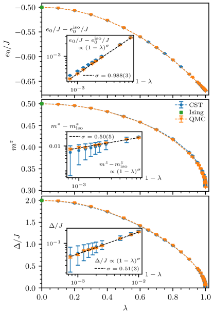
Repeating the estimates for the sublattice magnetization per site , we arrive at relative statistical QMC errors of order . In terms of the CST, the error of the finite-size effect and the effect of approximating a derivative by a ratio in the CST data is estimated as . The deviation between the data from QMC and CST becomes here maximal around as well and is of the order of , which is . This deviation, similarly to the deviation observed for the energy, does not change sign and evolves relatively smoothly. Thus, we presume that it is systematic and can be attributed to the CST truncation. Still, the agreement of the data from the two distinct approaches over the whole parameter range is very good.
Next, we address the value of the spin gap . The relative statistical errors of the QMC data are of order and near the isotropic Heisenberg point of order . The relative error estimate for the CST data yields and lower for and rises up to close to the isotropic point. While there is a small systematic deviation of the CST data, both approaches agree very well. We highlight that the double-logarithmic plot in the inset of the lowest panel in Fig. 1 displays an excellent agreement. Both data sets support the conclusion that the spin gap vanishes in a square root fashion , as reported in Refs. [40, 41]. Similarly, the magnetization approaches its value for the isotropic Heisenberg model also following a square root law.
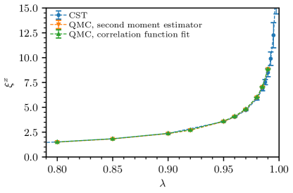
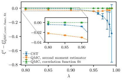
Finally, we consider the correlation length . Since we are dealing with a long-range ordered phase at all values of in the ground state of the Hamiltonian (1) this leads to an infinite (longitudinal) correlation length in the direction. But the magnons stand for transversal fluctuations of this order parameter. Hence, we consider the transversal correlation length pertaining to the dominantly exponential decay of for large values of .
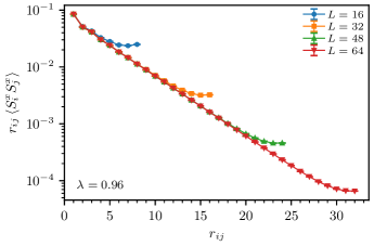
As shown in App. A for this two-dimensional system, an additional algebraic factor appears in the asymptotic scaling. We can demonstrate the above scaling behavior also based on QMC simulations. This is illustrated for the case of in Fig. 2. As we consider systems with periodic boundary conditions, the correlations for a system size are shown for distances . We find that the rescaled quantity approaches an exponential decay, as anticipated. By fitting the rescaled QMC data for to an exponential decay within the regime of between 5 and 20, we thus obtain a robust estimate for the correlation length in the TDL. We also used the improved second-moment estimator in Eq. 14 in order to obtain the correlation length from the structure factor which is extrapolated to the TDL including systems up to with . In CST, we describe the dispersion obtained numerically by a sum of cosine terms such that the dispersion is exactly captured. Then, we determine the correlation length by solving for the zeros in (18). Again, as shown in Fig. 3, the agreement is very good.
Concerning the power laws upon approaching the isotropic Heisenberg point, the CST and the QMC data sets strongly support the linear behavior of the ground-energy and square-root behavior for the sublattice magnetization, the spin gap, and the correlation length. The latter two power laws are not independent, but linked according to . All these power laws agree with the results of spin wave theory [40] which may appear surprising. But we emphasize that approaching the isotropic point does not represent a true quantum phase transition because the system stays in the same long-range ordered phase. The observed gap closure does not indicate a second order transition, but the restoration of the continuous symmetry of spin rotation which in turn implies the occurrence of Goldstone bosons. Since no critical quantum fluctuations appear the exponents remain the same as in mean-field theory. Our findings are further in agreement with very recent DMRG studies [42], that we became aware of during the completion of our manuscript.
IV Conclusions
In this paper we examined the ground-state properties of the anisotropic spin-1/2 Heisenberg AFM on the two-dimensional square lattice in the thermodynamic limit. For this purpose we considered two approaches, namely unbiased SSE QMC simulations as well as the semi-analytic CST method.
Based on our analysis of the ground-state energy , the excitation gap , the sublattice magnetization , as well as the transverse correlation length , we report a very good agreement of both approaches over the whole parameter range, from the Ising limit to the SU(2) symmetric isotropic Heisenberg point . Our findings support the quantitative validity of both approaches. In terms of the CST approach, this is particularly interesting as the method may be applied to extract quantum-critical properties as well as dynamical correlation functions of frustrated systems such as the - model or the Heisenberg model on the triangular lattice, where the statistical accuracy of QMC methods is severely limited, due to the sign problem.
Our data are available in [43] and provide quantitative reference results in the thermodynamic limit. We envision this to be of particular use for bench-marking purposes of numerical approaches for strongly correlated quantum spin systems.
Acknowledgements.
This work has been financially supported by the Deutsche Forschungsgemeinschaft (DFG, German Research Foundation) in project UH 90/14-1 (GSU) and SCHM 2511/13-1 (MRW/KPS) as well as the RTG 1995 (NC/SW). NC further acknowledges support by the ANR through grant LODIS (ANR-21-CE30-0033) and thanks the IT Center at RWTH Aachen University for access to computing time. KPS gratefully acknowledges the support by the Deutsche Forschungsgemeinschaft (DFG, German Research Foundation) – Project-ID 429529648—TRR 306 QuCoLiMa (“Quantum Cooperativity of Light and Matter”) and the Munich Quantum Valley, which is supported by the Bavarian state government with funds from the Hightech Agenda Bayern Plus. MRW/KPS thankfully acknowledge the scientific support and HPC resources provided by the Erlangen National High Performance Computing Center (NHR@FAU) of the Friedrich-Alexander-Universität Erlangen-Nürnberg (FAU).Appendix A Correlation function from the one-particle dispersion
This appendix contains a generalization of the results of Ref. [39] from one to any spatial dimension concerning the computation of the correlation length based on the full one-particle dispersion. In addition, we also derive the leading power law corrections.
We consider a translationally invariant system on a lattice in which the elementary excitations are bosonic and display a gap. Note that an ordered antiferromagnet on a bipartite lattice can be made translationally invariant by a rotation of the spins on one sublattice so that it belongs to the considered kind of systems. The Hamiltonian reads
| (19) |
where are the usual bosonic annihilation (creation) operators and an interaction term which needs not be specified further. The lattice constant is henceforth set to unity. Neglecting the interaction, the dispersion reads
| (20) |
and the correlation with is given at zero temperature by
| (21a) | ||||
| (21b) | ||||
If we include interaction effects, the functions and will be modified and hence . For simplicity, we refrain from introducing new labels for these modified quantities. In addition, Eq. (21b) does not hold anymore in a rigorous sense because of multi-boson contribution. But multi-boson contributions form continua in the space which induce dependences in real space which decay quicker than the contributions of the -distributions resulting from the single-boson states. However, the weights of the single-boson states are reduced due to hybridization with multi-boson states. Introducing a weight factor yields for the long-range part of the correlation
| (22) |
where we also left out the constant background stemming from the summand in (21b).
From (22) one realizes that a significant contributions results from small values of the dispersion. But this observation is not yet sufficient to find the correlation length. For this, the saddle point approximation needs to be invoked. For clarity, we first discuss the one-dimensional case, cf. Ref. 39.
One dimension
The dispersion can be described by a sum of trigonometric functions so that it is analytic. Note that the finite gap avoids the occurrence of singularities. The same holds true for the numerator . Then we can shift the integration from the real axis to a path in the complex plane crossing a point where
| (23) |
In order to deal with the singularity in the above integrand, we substitute by fulfilling
| (24) |
We denote by the point in with . The chain rule implies
| (25) |
By we denote the contour of which the image is the original contour, i.e., with and . Then we can write
| (26) |
This integration can be evaluated for by the saddle point approximation, also known as method of the steepest descent, yielding
| (27) |
where . With we obtain
| (28) |
For , we repeat the above reasoning for which also fullfills if the dispersion is even as is the case for systems with inversion symmetry.
We stress that the above derivation yields the power law correction in addition to the exponential decrease. Note that this power law differs from the classical Ornstein-Zernicke law [44].
Two dimensions
In essence, we repeat the arguments of the one-dimensional case. But the integration over the wave vectors is two-dimensional. We solve this issue by assuming rotational invariance of the asymptotic behavior in space, i.e., only matters. Correspondingly, we assume that the integrand in (22) is rotationally invariant in reciprocal space. This is not completely true, but can be justified a posteriori: we found that hardly depends on the direction or . The difference is only a few percent in the range and vanishes exponentially for larger correlation lengths.
Under the assumption of rotational invariance Eq. (22) becomes
| (29a) | ||||
| (29b) | ||||
The upper limit of the -integration is an approximation; but one does not need to bother because it does not enter the saddle point approximation. The function is the -th Bessel function of the first kind. Its asymptotic behavior for large arguments is
| (30) |
so that we can apply again the substitution and the saddle point approximation as in the one dimensional case yielding finally
| (31) |
with from as before. Note that the additional power law results from the asymptotic behavior of the Bessel function which in turn stems from the angular integration. It reflects how large the contribution of is.
Three dimensions
We repeat the arguments for the two-dimensional case. Assuming rotational invariance as in two dimensions the integration over the solid angle yields
| (32a) | ||||
| (32b) | ||||
As to be expected, the exponential dependence remains the same, but the power law exponent is lowered by . This leads us to
| (33) |
with from as before.
Arbitrary dimension
The obvious generalization of the above findings reads
| (34) |
in dimensions with from . Note that factors of in the denominator result from a phase space argument or geometrical dilution. But one factor stems from the saddle point approximation, see the derivation in one dimension.
Eq. (34) can be derived as before. First, we integrate in (22) over all angles at fixed modulus . We choose to point along so that and the angular integration yields
| (35a) | ||||
| (35b) | ||||
| (35c) | ||||
where we denoted for and used for the wave vector perpendicular to and the density of the modulus is given in dimension by . The integration over is carried out with the help of the -distribution yielding
| (36a) | ||||
| (36b) | ||||
| (36c) | ||||
| (36d) | ||||
where we substituted . In the final integration over , we use again the asymptotics (30) and employ the saddle point approximation to obtain (34) stated above.
Appendix B QMC estimator for the correlation length
In this appendix, we discuss the QMC estimator for the correlation length in different spatial dimensions and for different correlation function asymptotics. In the case of the Ornstein-Zernike form of the correlation function [44] in spatial dimensions, , the improved second-moment estimator reads
| (37) |
as discussed in Ref. [23] (note that there is an apparent typo in Eq. (71) of Ref. [23]). The numerical prefactor in the above estimator is of order one and thus often ignored when extracting correlation lengths based on this estimator. Indeed, for and the prefactor simplifies to exactly, while for it reads , explicitly. For other algebraic factors in the correlation function asymptotics, the numerical prefactor however differs. In particular, for the asymptotic behavior derived in the preceding appendix we similarly obtain, upon analytically performing the Fourier transformation in the continuum limit, the corresponding prefactors , , and for , respectively.
Appendix C Quantitative comparison of CST and QMC results
Here, we show a quantitative comparison of the CST and QMC results in terms of the statistical and systematic errors. In Fig. 4 the deviations of the CST data relative to the QMC data is plotted for the ground-state energy per site , the magnetization per site , and the energy gap . In energy and magnetization the deviation is remarkably small for small values of growing for large . We attribute this to the truncation of the tracked terms on quartic level corresponding to scaling dimension . Hence, it is a systematic deviation which we had observed before in the binding energies of two-magnon bound states [10]. We do not have a complete understanding of the deviations of the spin gap which is rather constant. Still, we presume a systematic origin linked to the truncation in the CST approach. Remarkably, the deviations decrease in all three quantities upon approaching the isotropic point. We interpret this as a justification of the truncation according to scaling dimension which allows us to find the relevant effective model close to the isotropic point almost quantitatively.
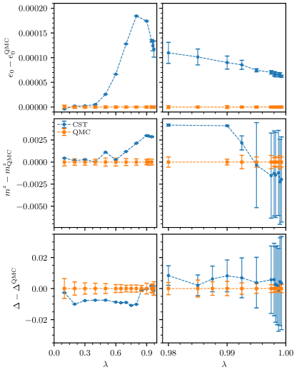
Finally, Fig. 5 displays the deviation of three ways to access the transversal correlation length. The two QMC estimators agree well below the one percent level. Such minor deviations may result from uncertainties in performing the actual finite-size fitting process. The CST results acquire large errors close to the isotropic point because the correlation length depends inverse proportionally on the spin gap so that tiny inaccuracies in the latter induce large inaccuracies in the correlation length.
References
- Chappert et al. [2007] C. Chappert, A. Fert, and F. Van Dau, The emergence of spin electronics in data storage, Nature Materials 6, 813 (2007).
- Baltz et al. [2018] V. Baltz, A. Manchon, M. Tsoi, T. Moriyama, T. Ono, and Y. Tserkovnyak, Antiferromagnetic spintronics, Review Modern Physics 90, 015005 (2018).
- Gomonay et al. [2017] O. Gomonay, T. Jungwirth, and J. Sinova, Concepts of antiferromagnetic spintronics, Physica Status Solidi - Rapid Research Letters 11, 1700022 (2017).
- Bednorz and Müller [1986] J. G. Bednorz and K. A. Müller, Possible High- Superconductivity, Zeitschrift der Physik B 64, 189 (1986).
- Manousakis [1991] E. Manousakis, The Spin- Heisenberg Antiferromagnet on a Square Lattice and its Application to the Cuprous Oxides, Review Modern Physics 63, 1 (1991).
- Auerbach [1994] A. Auerbach, Interacting Electrons and Quantum Magnetism, Graduate Texts in Contemporary Physics (Springer, New York, 1994).
- Powalski et al. [2015] M. Powalski, G. S. Uhrig, and K. P. Schmidt, Roton Minimum as a Fingerprint of Magnon-Higgs Scattering in Ordered Quantum Antiferromagnets, Physical Review Letters 115, 207202 (2015).
- Verresen et al. [2018] R. Verresen, F. Pollmann, and R. Moessner, Quantum dynamics of the square-lattice Heisenberg model, Physical Review B 98, 155102 (2018).
- Powalski et al. [2018] M. Powalski, K. P. Schmidt, and G. S. Uhrig, Mutually attracting spin waves in the square-lattice quantum antiferromagnet, SciPost Phys. 4, 1 (2018).
- Walther et al. [2023] M. R. Walther, D.-B. Hering, G. S. Uhrig, and K. P. Schmidt, Continuous similarity transformation for critical phenomena: easy-axis antiferromagnetic XXZ model, Physical Review Research 5, 013132 (2023).
- Schmiedinghoff et al. [2022] G. Schmiedinghoff, L. Müller, U. Kumar, G. S. Uhrig, and B. Fauseweh, Three-body bound states in antiferromagnetic spin ladders, Communications Physics 5, 218 (2022).
- Knetter et al. [2001] C. Knetter, K. P. Schmidt, M. Grüninger, and G. S. Uhrig, Fractional and integer excitations in quantum antiferromagnetic spin ladders, Physical Review Letters 87, 167204 (2001).
- Windt et al. [2001] M. Windt, M. Grüninger, T. Nunner, C. Knetter, K. P. Schmidt, G. S. Uhrig, T. Kopp, A. Freimuth, U. Ammerahl, B. Büchner, and A. Revcolevschi, Observation of two-magnon bound states in the two-leg ladders of (Ca,La)14Cu24O41, Physical Review Letters 87, 127002 (2001).
- Notbohm et al. [2007] S. Notbohm, P. Ribeiro, B. Lake, D. A. Tennant, K. P. Schmidt, G. S. Uhrig, C. Hess, R. Klingeler, G. Behr, B. Büchner, M. Reehuis, R. I. Bewley, C. D. Frost, P. Manuel, and R. S. Eccleston, One- and two-triplon excitations of an ideal spin-ladder, Physical Review Letters 98, 027403 (2007).
- Tseng et al. [2023] Y. Tseng, E. Paris, K. P. Schmidt, W. Zhang, T. C. Asmara, R. Bag, V. N. Strocov, S. Singh, J. Schlappa, H. M. Rønnow, S. Johnston, and T. Schmitt, Momentum-resolved spin-conserving two-triplon bound state and continuum in a cuprate ladder, Communications Physics 6, 138 (2023).
- Sandvik and Kurkijärvi [1991] A. W. Sandvik and J. Kurkijärvi, Quantum Monte Carlo simulation method for spin systems, Physical Review B 43, 5950 (1991).
- Sandvik [1999] A. W. Sandvik, Stochastic series expansion method with operator-loop update, Physical Review B 59, R14157 (1999).
- Syljuåsen and Sandvik [2002] O. F. Syljuåsen and A. W. Sandvik, Quantum monte carlo with directed loops, Phys. Rev. E 66, 046701 (2002).
- Alet et al. [2005] F. Alet, S. Wessel, and M. Troyer, Generalized directed loop method for quantum Monte Carlo simulations, Physical Review E 71, 036706 (2005).
- Sandvik [1997a] A. W. Sandvik, Finite-size scaling of the ground-state parameters of the two-dimensional Heisenberg model, Physical Review B 56, 11678 (1997a).
- Singh [1989] R. R. P. Singh, Thermodynamic Parameter of the , Spin- Square-Lattice Heisenberg Antiferromagnet, Physical Review B 39, 9760 (1989).
- Dusuel et al. [2010] S. Dusuel, M. Kamfor, K. P. Schmidt, R. Thomale, and J. Vidal, Bound states in two-dimensional spin systems near the Ising limit: A quantum finite-lattice study, Physical Review B 81, 064412 (2010).
- Sandvik [2010] A. W. Sandvik, Computational Studies of Quantum Spin Systems, AIP Conference Proceedings 1297, 135 (2010).
- Evertz [2003] H. G. Evertz, The loop algorithm, Advances in Physics 52, 1 (2003).
- Swendsen and Wang [1987] R. H. Swendsen and J.-S. Wang, Nonuniversal critical dynamics in Monte Carlo simulations, Physical Review Letters 58, 86 (1987).
- Kawashima and Gubernatis [1995] N. Kawashima and J. E. Gubernatis, Dual Monte Carlo and cluster algorithms, Physical Review E 51, 1547 (1995).
- Caci et al. [2021] N. Caci, L. Weber, and S. Wessel, Hierarchical single-ion anisotropies in spin-1 Heisenberg antiferromagnets on the honeycomb lattice, Physical Review B 104, 155139 (2021).
- Liu [2024] L. Liu, Improvements to the stochastic series expansion method for the model with a magnetic field, Physical Review B 109, 045141 (2024).
- Suwa and Todo [2015] H. Suwa and S. Todo, Generalized Moment Method for Gap Estimation and Quantum Monte Carlo Level Spectroscopy, Physical Review Letters 115, 080601 (2015).
- Sandvik [1997b] A. W. Sandvik, Finite-size scaling of the ground-state parameters of the two-dimensional Heisenberg model, Physical Review B 56, 11678 (1997b).
- Reger and Young [1988] J. D. Reger and A. P. Young, Monte Carlo simulations of the spin-1/2 Heisenberg antiferromagnet on a square lattice, Physical Review B 37, 5978 (1988).
- Dorneich and Troyer [2001] A. Dorneich and M. Troyer, Accessing the dynamics of large many-particle systems using the stochastic series expansion, Physical Review E 64, 066701 (2001).
- Dyson [1956] F. J. Dyson, General theory of spin-wave interactions, Physical Review 102, 1217 (1956).
- Maleev [1958] S. V. Maleev, Scattering of slow neutrons in ferromagnets, Soviet Physics JETP 6, 766 (1958).
- Wegner [1994] F. Wegner, Flow equations for hamiltonians, Ann. Physik 506, 77 (1994).
- Kehrein [2006] S. Kehrein, The Flow Equation Approach to Many-Particle Systems, Springer Tracts in Modern Physics, Vol. 217 (Springer, Berlin, 2006).
- Knetter and Uhrig [2000] C. Knetter and G. S. Uhrig, Perturbation theory by flow equations: dimerized and frustrated chain, European Physical Journal B 13, 209 (2000).
- Fischer et al. [2010] T. Fischer, S. Duffe, and G. S. Uhrig, Adapted continuous unitary transformation to treat systems with quasi-particles of finite lifetime, New Journal of Physics 10, 033048 (2010).
- Okunishi et al. [2001] K. Okunishi, Y. Akutsu, N. Akutsu, and T. Yamamoto, Universal relation between the dispersion curve and the ground-state correlation length in one-dimensional antiferromagnetic quantum spin systems, Physical Review B 64, 104432 (2001).
- Hamer et al. [1992] C. J. Hamer, Z. Weihong, and P. Arndt, Third-order spin-wave theory for the Heisenberg antiferromagnet, Physical Review B 46, 6276 (1992).
- Zheng et al. [2005] W. Zheng, J. Oitmaa, and C. J. Hamer, Series studies of the spin- Heisenberg antiferromagnet at : Magnon dispersion and structure factors, Physical Review B 71, 184440 (2005).
- Kadosawa et al. [2024] M. Kadosawa, M. Nakamura, Y. Ohta, and S. Nishimoto, Comparing quantum fluctuations in the spin- and spin- XXZ Heisenberg models on square and honeycomb lattices (2024), arXiv:2404.08099 .
- Caci et al. [2024] N. Caci, D.-B. Hering, M. Walther, K. P. Schmidt, S. Weßel, and G. Uhrig, Figure data to ”Quantitative decription of long- range order in the anisotropic spin-1/2 Heisenberg antiferromagnet on the square lattice”, 10.5281/zenodo.11189975 (2024).
- Cardy [1996] J. Cardy, Scaling and Renormalization in Statistical Physics, Cambridge Lecture Notes in Physics (Cambridge University Press, 1996).