The role of sunspots magnetic configuration in the formation of umbral fine-structures

Abstract

We use spectro-polarimetric data recorded by Hinode to analyze the magnetic field configuration of a part of a sunspot (AR 10923) where a bundle of penumbral filaments are intruding into its umbra. We want to explore the role of the sunspot magnetic configuration in the formation and kinematics of the fine-structures, such as umbral dots and light bridges, inside the sunspot umbra. Both direct inferences from polarization Stokes profiles and the inversion results using the SIR code indicate an aligned magnetic field configuration in the umbra where moving umbral dots are easily formed at the leading edges of the rapidly intruding penumbral filaments. We suggest that the magnetic field topology is rearranged leading to the observed aligned magnetic field lines via magnetic reconnection process by which a part of the magnetic energy is converted into thermal and kinetic energy. This new configuration causes the umbral fine-structures to form easily and more frequent.

1 Introduction

Sunspots, the darkest regions on the solar surface, are understood to be the result of partially inhibiting heat transfer from the solar interior to the surface by strong magnetic fields [1, 2]. The investigation of the bright fine-structures formed inside sunspot umbrae, like umbral dots or light bridges (LBs), are important to understand the physical mechanisms responsible for the heat transfer into the photosphere and for the magnetic field energy dissipation in atmospheric layers. LBs are lanes of relatively bright and hot plasma dividing sunspot umbrae into two parts and displaying a large variety of morphology and fine structure [3] and can be seen during both formation and decaying of a sunspot (for a review see [4]).

The origin of dark cores/lanes observed in bright penumbral filaments [5] as well as in LBs in continuum and polarization maps was theoretically described by Ruiz Cobo & Bellot Rubio [6]: a dark core is a consequence of the higher density of the plasma inside penumbral filament, which shifts the surface of optical depth unity toward higher (cooler) layers.

It is still unknown what triggers the formation of an LB, and what is the role of the penumbra in the development of an LB [7] and in the formation of umbral dots [7, 8] and their kinematics [9, 10].

In this paper, the umbral magnetic structure around a bundle of penumbral filaments intruding into a sunspot umbra is investigated using spectro-polarimetric measurements from the Japanese satellite Hinode [11]. In the studied umbral area, a long and faint filamentary LB (as classified by Sobotka [3]) is seen.

2 Data Set

The data analyzed here were obtained using the spectro-polarimeter of the Solar Optical Telescope (SOT: [12, 13]) onboard Hinode satellite. The instrument observes the two iron lines Fe I 630.15 nm ($g=1.67$) and Fe I 630.25 nm ($g=2.5$), whose line formation region is between $\log(\tau)\approx 0$ and $-3$. A normal full-field scan of AR 10923 was taken on 15 November 2006, during the period 03:15 - 03:52 UT, when the spot was located at the heliocentric angle of $13^{\circ}$. From this scan, a field of $20\times 20$ arcsec ², corresponding to 130 consecutive slit positions and containing the part of the penumbra intruding into the umbra, was selected for further analysis. The continuum intensities of the Stokes I profiles from the pixels with low polarization signals in the whole field of view and the known limb darkening function were used to find the continuum intensity of the quiet Sun at disk center to normalize all Stokes profiles. The sunspot has negative magnetic polarity, and then the regular Stokes V profiles have negative blue lobes.

Figure 1 shows the intensity map of the sunspot as reconstructed from the continuum intensities of the Stokes I profiles. The area ($130\times 130$ pixels) analyzed here is shown by a white square in Figure 1. This area contains a long filamentary light bridge (LB), a part of the penumbra intruding into the umbra and some individual umbral dots (UDs) and chains of them. The formation process of this LB was studied by Katsukawa et al. [7]. They suggested that the continual emergence of umbral dots from the leading edges of penumbral filaments as well as their rapid inward migration forms the LB inside the umbra.

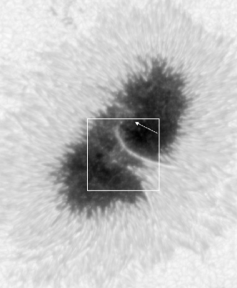
Figure 1: The continuum intensity map reconstructed from the continuum of the Stokes I profiles. The size of the image is $430\times 520$ pixels, equivalent to $68\times 82$ arcsec². The size of analyzed region (white square) is $130\times 130$ pixels, equivalent to $20\times 20$ arcsec². The arrow points to solar disk center.

3 Direct Inferences from Observed Stokes Profiles

3.1 Fine structures of the filamentary light bridge

As observed with Hinode [14] and the SST [15], dark cores is more prominent in polarized light (Stokes Q, U and V) than in continuum intensity. However, Bellot Rubio et al. [14] found weaker dark core polarization signals. Their inversion results indicate that dark cores have weaker and more inclined magnetic fields.

Figure 2 shows the continuum intensity map as well as the maps of Stokes Q, U and V computed from 630.25 nm line. Here Q and U refer to the signal values of the $\pi$ component of the corresponding Stokes parameters (signal at the line core), and V refers to the (negative) amplitude of the blue lobe of Stokes V profile. We cannot clearly resolve any dark core on the filamentary LB in the continuum intensity map [6] (see upper-left panel in Figure 2). Figure 3 shows total polarization (TP $=\sum_{\lambda}{\sqrt{Q^{2}+U^{2}+V^{2}}}$), left panel) and total circular polarization (TCP $=\sum_{\lambda}{|V|}$), right panel) maps, both constructed from the 630.25 nm line. Although spatial resolution of Hinode/SP observations is not quit high, however, in some Stokes polarization maps, we can clearly resolve dark core on the filamentary LB as well as on other intruding filaments at the lower-right corner of the studied area [14, 15]: stronger signals in Stokes V and U (upper- and lower-right panels in Figure 2, respectively), weaker signals in TP and TCP maps (left and right panels in Figure 3, respectively). However, as can be seen in the lower-left panel in Figure 2, the dark core in the map of Stokes Q signals has a different display: The core of the LB appears as a sharp border dividing positive and negative signals.

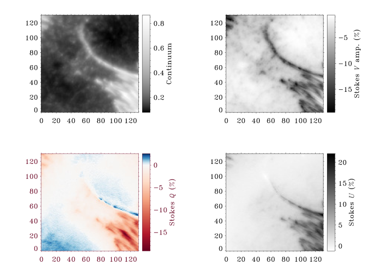
Figure 2: Left to right, top to bottom: continuum intensity map, the map of Stokes V amplitude, and the maps of Q and U signals at the line core. All maps are reconstructed from the 630.25 nm line and normalized to the quiet Sun continuum intensity at disc center.

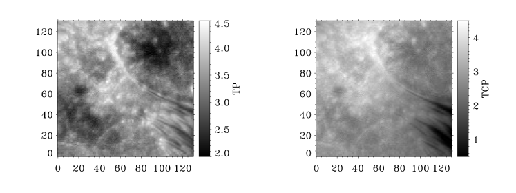
Figure 3: Left panel: total polarization map. Right panel: total circular polarization map. All maps are reconstructed from the 630.25 nm line and normalized to the quiet Sun continuum intensity at disc center.

3.2 Other fine structures

All bright structures especially umbral dots resolved in the map of continuum intensity (upper-left panel in Figure 2) are more pronounced in TP map (left panel in Figure 3). A faint tinny arced structure seen at the lower half of the continuum intensity map can also be recognized in the maps of Stokes V (Figure 2) as well as in the maps of TP and TCP (Figure 3). Also a few chains of small umbral dots are seen at the center of the maps of continuum intensity, Stokes V signals and TP.

As mentioned before, the maps displayed in Figures 2 and 3 were computed from the 630.25 nm line. The corresponding maps derived from the 630.15 nm line are very similar to the ones reconstructed from the 630.25 nm line. We concentrate on the results of the 630.25 nm line which is a triplet Zeeman line.

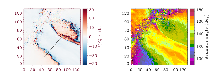
Figure 4: Left panel: the map of U/Q ratio. The dashed line shows a cut across the region whose polarization signals are displayed in Figure 5. Right panel: the map of the azimuth angle of the magnetic field vector estimated from $\tan(2\varphi)=U/Q$. We did not correct the $180^{\circ}$ ambiguity in azimuth angle in the upper-left corner of the studied area.

3.3 Azimuth angle of the magnetic field

The map of Stokes Q signals shown in the lower-left panel in Figure 2 needs special attention. This map shows a distinct (red) region having negative values extended from the center of the map to the lower-right corner including the bright structures (penumbral grains and filaments) seen in the continuum intensity map. This may be questioned that this behavior is the natural consequence of the measured Stokes Q or Uon a fanning magnetic structure of a sunspot in Hinode/SP observations. However, both lower and upper seen boundaries cannot be explained. To investigate what happened in this region we compute the ratio of U/Q which scales with $\tan(2\varphi)$ in which $\varphi$ is the azimuth angle of the magnetic field vector [16, 17]. The left panel in Figure 4 displays the map of this ratio in which the distinct region with a clearly sharp boundary is seen as it was observed in the map of Stokes Q signals (lower-left panel in Figure 2). The upper boundary of the region is co-spatial with the filamentary LB. The map of the azimuth angle of the magnetic field vector estimated using $\tan(2\varphi)=U/Q$ is shown in the right panel in Figure 4. We do not resolve the $180^{\circ}$ azimuth ambiguity in the upper-left corner where is not area of interest.

Figure 5: Line core signals of Stokes Q and U (upper panels), and the values of U/Q ratio (lower-left panel) along the cut shown by dashed-line in Figure 4. Lower-right panel: the plot of the azimuth angle ($\varphi$) of the magnetic field along the cut, estimated from $\tan(2\varphi)=U/Q$.

Figure 5 shows the variations of the signals of Stokes Q and U (upper-left and -right panels, respectively), and values of the U/Q ratio (lower-left panel) along the shown cut across the distinct region (see Figure 4). The magnetic field azimuth angles along the cut, estimated using $\tan(2\varphi)=U/Q$ are also shown in the lower-right panel in Figure 5. The signals of Stokes Q (upper-left panel) are positive outside the distinct region, decreasing to zero where borders are defined. Entering the distinct region, the signals of Stokes Q show negative non-zero values. Stokes U signals (upper-right panel) are positive inside and outside of the distinct region. The different values of the U/Q ratio outside and inside the distinct region define different azimuth angles for the magnetic field vectors around the border of the distinct region.

Figure 6 displays the full Stokes profiles for three pixels around the lower boundary of the distinct region on the defined cut. We can see the changes of the signal at the line core of Stokes Q when passing the boundary.

Looking at the right panel in Figure 4, we can see that the distinct region show an area where the magnetic field vectors have almost the same azimuth angles implying aligned magnetic field vectors. This means that the magnetic field vector noticeably rotates by changing its azimuth upon entering the distinct region. This can be an evidence for a process rearranging the magnetic field vectors in the distinct region. In other words, the magnetic field vectors tend to be well-arranged there.

Figure 6: The profiles of Stokes I, Q, U and V for three selected pixels on the cut shown by dashed-line in Figure 4 at intersecting the lower border of the distinct region. Upper (lower) panels: Stokes profiles for a pixel outside (inside) the distinct region. Middle panels: Stokes profiles for a pixel on the border. The vertical dashed lines show the line core and $\pm 215$ mÅ around it in both spectral lines.

4 Inversion Results

To have a confirmation for the direct inferences we applied the inversion code SIR (Stokes Inversion based on Response functions [18]) to the observed spectra. Inversions were made for a single-component magnetic model atmosphere. As discussed by Sobotka & Jur$\check{c}\acute{a}$k [19], the instrumental scattered light is negligible in Hinode/SP data.

Blending spectral lines are more prominent in Stokes profiles observed in a sunspot umbra (see the left panels in Figure 6). As shown by Hamedivafa [20] the unknown blending lines broaden the recovered Stokes I cause a higher macro/microturbulent velocity and give smaller near-continuum intensity, resulting in slightly cooler temperature stratification at least in deeper layers. Therefore, the code ignores the blended parts of the spectral lines (see Figure 9 in [20]) to recover a better fitted profile and to retrieve a more reliable atmospheric model.

To detect the changes of temperature with height, we used five nodes for temperature and two nodes for LOS velocity and magnetic field strength in the final step of the inversion process. Furthermore, to find effective values for the magnetic field inclination and its azimuth angle, we considered them height-independent (one node). Additionally, we enabled one node for micro-turbulent velocity. The weights of Stokes I, Q, U and V were adopted to be equal in the inversion.

Figure 7 displays the retrieved photospheric model at optical depth of $-0.4$. Although the temperature (T) map is similar to the intensity map shown in Figure 2, however, in the temperature (T) map we can recognize dark cores on the penumbral filaments with a good contrast. Velocities have been calibrated considering zero velocity for the umbral core region. In the velocity map (V), adjacently localized small patches showing up- and down-flows are seen on the LB implying a multi-segmented structure for it [21]. This structure is similar to the multi-cell convection pattern for light bridges suggested by Jingwen Zhang et al. [22]. Penumbral grains, the bright head of the intruding penumbral filaments, show upflows up to 400 m s^-1, although the signature of the p-mode oscillations enters a perturbation in the velocity map. Also, at the lower-right side of the studied area, the LOS component of the outward Evershed flow [1] is seen as downflows along the intruding penumbral filaments. Magnetic field on the core of bright filamentary structures and penumbral grains is weaker (B map) and more inclined (Gamma map) than that in their surroundings. This view is consistent with the inversion results of Bellot Rubio et al. [14]. The curved filamentary LB has a signature in the map of azimuth angle as well. Here, also we did not correct the $180^{\circ}$ azimuth ambiguity in the upper-left corner of the studied area. The distinct region shows a uniform azimuth angle but different (in average, $15^{\circ}$ larger) with the azimuth of the surrounding filed.

The variations of the azimuth angle across the distinct region along the defined cut shown in lower-middle panel in Figure 7 (the same as shown in Figure 4) are plotted in the lower-right panel in Figure 7. These variations are very similar to the corresponding variations plotted in the lower-right panel in Figure 5, although the values have a difference of about $10^{\circ}$, in average. The difference arises from the different ways obtaining the azimuth. In direct inference we used the amplitudes of Stokes Q and U at the line center and in inversion we adopted a height-independent azimuth. The inversion results confirm the direct inferences for azimuth angle shown in Figures 4 and 5. Also, the distinct region shows itself in the inclination map (Gamma) as a region with an equalized inclination angle.

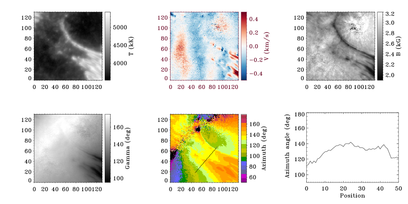
Figure 7: Upper panels, left to right: maps of temperature (T), magnetic field strength (B), LOS velocity (V). Negative velocities (blue) are upflows. Lower-left and -middle panels: maps of inclination (Gamma) and azimuth angle at optical depth of $-0.4$. Lower-right panel: the graph of azimuth angles derived from the retrieved atmospheric model across the distinct region along the cut shown in the azimuth panel.

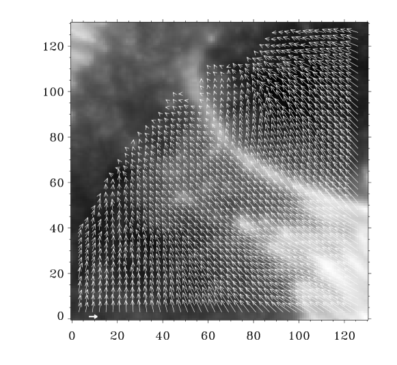
Figure 8: The projection of the magnetic field vectors in the plane perpendicular to the LOS. Horizontal vector at the lower-left corner of the map displays the unit vector (1 kG).

Figure 8 shows the projection of the magnetic field vector in the plane perpendicular to the LOS. Since the sunspot is close to the solar disc center, it does not need the magnetic field vectors to be transferred from the LOS reference frame into the local (disc center) reference frame. Inside the distinct area, field vectors are (orderly) aligned as we deduced in Section 3.3.

5 Summary and Conclusion

Here we presented an investigation of SP observations recorded by Hinode/SOT from a part of sunspot umbrae (AR 10923). The studied area contains a long filamentary light bridge (LB), penumbral filaments intruding into the umbrae and umbral dots. The spot was located close to the disk center. Our investigation consists of the results of both direct analysis of Stokes spectra and inversion using SIR code. In this study, we explore the role of the penumbra in the formation and kinematics of umbral dots and LBs.

Katsukawa et al. [7] studied the formation process of the LB observed in our studied area. They pointed out that during the formation of the LB, many umbral dots were observed, emerging from the leading edges of the rapidly intruding penumbral filaments. They identified central umbral dots formed inside the umbra with a relatively slow inward motion as the precursor of the LB formation. But, what process causes mobile umbral dots to be easily formed inside the umbra. They suggested that the emergence and the inward motion of the central umbral dots are triggered by a buoyant penumbral flux tube as well as upward subphotospheric flows reaching the surface.

Our study shows that umbral dots and intruding penumbral filaments reside in a distinct region where the magnetic field vectors are rearranged so that their azimuths as well as inclinations are equalized. The LB forms one boundary of the distinct region. We suggest the orderly rearranging of the magnetic field vectors is the reason of the easily formation of the umbral dots and their slow inward motion observed by Katsukawa et al. [7].

Chromospheric observations reveal long-lasting recurring jet-like activities above light bridges (e.g., [23, 24]) or inverted Y-shaped magnetic structures in a penumbral region [25] and a penumbral intrusion into the umbra [26]. These are usually suggested to be a natural consequence of magnetic reconnection by which a part of the magnetic energy is converted into thermal and kinetic energy (e.g., [27]). Therefore, the magnetic field topology is rearranged via magnetic reconnection process. This rearrangement may lead to a well-arranged magnetic field configuration. Therefore, it is also important to study the photospheric and chromospheric magnetic configuration of a sunspot before intruding penumbral filaments into the umbra to confirm this suggestion.

References

- [1] Solanki S. K., 2003, A&ARv 11, 153
- [2] Rempel M., et al., 2009, Science 325, 171
- [3] Sobotka M., 1997, in ASP Conf. Ser. 118, “1st Advances in Solar Physics Euroconference. Advances in Physics of Sunspot”, ed. B. Schmieder, J. C., del Toro Iniesta, and M. Vazquez (San Francisco, CA: ASP), 155
- [4] Moradi H., et al., 2010, Solar Phys. 267, 1
- [5] Scharmer G. B., et al., 2002, Nature 420, 151
- [6] Ruiz Cobo B., and Bellot Rubio L.R., 2008 A&A 488, 749
- [7] Katsukawa Y., et al., 2007, PASJ 59, 577
- [8] Schussler M., and Vgler A., 2006, ApJ 641, L73
- [9] Sobotka M., Brandt P. N., and Simon G. W., 1997, A&A 328, 689
- [10] Watanabe H., et al., 2010, Solar Phys. 266, 5
- [11] Kosugi T., et al., 2007, Solar Phys. 243, 3
- [12] Tsuneta S., et al., 2008, Solar Phys. 249, 167
- [13] Suematsu Y., et al., 2008, Solar Phys. 249, 197
- [14] Bellot Rubio L. R., et al., 2007, ApJ 668, L91
- [15] van Noort M., and Rouppe van der Voort L. H. M., 2008, A&A 489, 429
- [16] Auer L. H., Hgasley J. N., and House L. L., 1977, Solar Phys. 55, 47
- [17] Stenflo J. O., 2013, A&ARv 21, 66
- [18] Ruiz Cobo B., and del Toro Iniesta J. C., 1992, ApJ 398, 375
- [19] Sobotka M., and Jurk J., 2009, ApJ 694, 1080
- [20] Hamedivafa H., 2013, Solar Phys. 286, 327
- [21] Thomas J. H., and Weiss N. O., 2004, ARA&A 42, 517
- [22] Zhang J., et al., 2018, ApJ 865, 29
- [23] Roy J. R. 1973, Solar Phys. 28, 95
- [24] Song D., et al., 2017, ApJ 835, 240
- [25] Zeng Z., et al., 2016, ApJL 819, L3
- [26] Bharti L., Solanki S. K., and Hirzberger J., 2017, A&A 597, 127
- [27] Zhang T. L., et al., 2012, Science 336, 567