Near critical asymptotics in the Frozen Erdős-Rényi
Abstract
We consider a variant of the classical Erdős-Rényi random graph, where components with surplus are slowed down to prevent the apparition of complex components. The sizes of the components of this process undergo a similar phase transition to that of the classical model, and in the critical window the scaling limit of the sizes of the components is a "frozen" version of Aldous’ multiplicative coalescent [2]. The aim of this article is to describe the long time asymptotics in the critical window for the total number of vertices which belong to a component with surplus.
1 Introduction
We are interested in a modification of the classical Erdős-Rényi random graph, the frozen Erdős-Rényi (introduced in [8]), the general idea of which is to obtain a simple graph, that is, without complex components (with surplus larger than ). This model is in the vein of numerous variants of the classical model, which have been introduced to see how phase transition is transposed through modification. Indeed it is well known [9] that the components’ sizes of the Erdős-Rényi random graph with vertices and edges exhibits a phase transition at . More precisely, when with the largest component is of size whereas a giant component emerges in the supercritical case . The critical window has also been widely studied and when the components are of order (see e.g. [4], [17], [18] for full literature on the subject). Complex components of the classical model are also well understood: they are rare in the subcritical phase, and the giant component is practically the only complex component in the supercritical phase. This predominance of simple components (trees or unicycles) in the classical model motivates the study of this modified model which results in a simple graph.
The frozen graph also resonates with several variants of the classical model which have been introduced to observe how perturbations affect the phase transition. For example, in 2000, Achlioptas suggested a class of variants, where at each step the added edge is chosen from two uniform random edges, according to a certain rule (see e.g. [1]). These models were introduced in particular to study discontinuous phase transitions [1], but Riordan and Warnke [23] have in fact proved that the resulting phase transition is similar to that of the classical model. An other example is Ráth and Tóth’s "forest fires" model [22] where they add the possibility for components to "burn" and for which they prove a self-organized criticality. We thus are interested in understanding the phase transition for the frozen Erdős-Rényi model.
Let us first recall properly the classical model: consider independent identically distributed unoriented edges , where both endpoints are independent and uniform over (notice that we may have for or ). For , the Erdős-Rényi random graph is the (multi)graph whose vertices are and whose edges are . The frozen Erdős-Rényi process depends on a parameter and is constructed as follows: for , still is the set of vertices, which are of two types: standard or frozen. Initially is made of the standard isolated vertices . We use the same edges as in the Erdős-Rényi model (which gives us a coupling between both processes) and let a sequence of independent identically distributed variables with uniform law over , which are also independent of the . We construct the process according to the following rules:
-
•
if connects two trees, the edge is added to to form . If this addition creates a cycle in the tree, we declare the new component frozen.
-
•
if both endpoints of are frozen, then is discarded and
. -
•
if connects a tree and a unicycle, then is discarded if and kept otherwise. If is kept the new connected component is declared frozen.
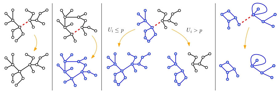
Notice that frozen components are exactly unicycles and that the resulting graph has no complex components. For , the process corresponds to a complete stop in the progression of component with surplus, while for the process is obtained from by discarding the edges which would create a surplus of . The case is therefore intimately tight to the classical Erdős-Rényi random graph since both graphs coincide on the "forest part", and the number of vertices which belongs to a component with surplus in is the same as the number of frozen vertices in . The frozen Erdős-Rényi has been introduced by Contat and Curien in [8] in the case , where they constructed a coupling between and a model of random parking on uniform Cayley trees. They only studied in details the case but their results can be generalized without additional difficulty for general , we prove it rigorously in [26] (in preparation).
The sizes of the components of the frozen process undergoes a phase transition when , similar to that of the classical Erdős-Rényi process. In this model, the number of frozen vertices becomes macroscopic in the supercritical regime. The model is also of interest to physicists: Krapivksy [15] studies the number of frozen vertices and gives a differential equation for its scaling limit in the supercritical regime. We focus here on the critical window : in a similar way to the work of Aldous [2], [8] proves a convergence of the renormalized sizes of the components when for Inspired by this critical window, we shall note
the continuous-time version of the process, and the process of the decreasing sizes of the frozen components (completed with zeros) renormalized by followed by the decreasing sizes of the standard components renormalized by (also completed with zeros) in . In the critical regime, the process converge towards a process called the frozen multiplicative coalescent (which is a modification of Aldous’ multiplicative coalescent [2], as we will see in Section 5). As an immediate consequence, in the critical window, the total number of frozen vertices renormalized by converges to a process and it has been shown in [8] that is an inhomogeneous pure jump Feller process whose jump kernel is given by :
| (1.1) |
where is the time parameter, the space parameter and the size of the jump and where is the density of a spectrally positive stable distribution of parameter :
| (1.2) |
where Ai is the Airy function (see [25] for a definition). Here again these results are proved in details for in [8] and are generalized rigorously using the same tools in [26].
The process is the main object of this article: we are interested in the number of frozen vertices at the frontier of the critical window (the so-called near supercritical regime). With the previous description of , Contat and Curien [8] conjectured that for all :
The aim of this article is to prove this conjecture, and actually demonstrates a stronger concentration of the process around the line . We distinguish the case from the other cases since the proofs use different tools and arguments. Our two main results are as follows.
Theorem 1.1.
For all we have the following convergence:
The case is intimately tight to the standard Erdős-Rényi, in this case Theorem 1.1 informally states that the number of frozen vertices in is approximatively when is large and goes to . This has to be related to Luczak’s result [17] saying that the size of largest cluster in is close to when goes to : this largest cluster is indeed likely to be formed by the majority of unicycles in the frozen Erdős-Rényi of parameter . For we prove the following.
Theorem 1.2.
For , the process is positive recurrent and converges at an exponential rate to an invariant probability measure on .
Furthermore, verifies the following tail inequality: there exists such that for all :
This theorem has an interesting consequence on the frozen Erdős-Rényi graph with parameter : it implies the convergence of its forest part to a stationary law at the frontier of the critical window. For this corollary we note the scaling limit of the renormalized components’ sizes of the forest part in the frozen graph with parameter (this notation will be justified in Section 5).
Corollary 1.3.
For all , we have the following convergence in distribution for the topology
where is a random variable with distribution .
This is an example of "self-organized criticality" (see e.g. [22] for the forest fire model, and [7] for examples in percolation theory), since when the forest is not attracted by frozen particles (edges between trees and unicycles are forbidden). Thus the only way for a tree to freeze is to create an internal cycle. When , the attraction of the freezer foster freezing of small trees, making a self-organized criticality impossible. More generally, we will give in Section 5 a description of the scaling limit of the frozen graph, and give a new description of particles with surplus in Aldous’ augmented multiplicative coalescent (Corollary 5.2). This section also involves scaling limits of critical random forests, studied by Martin and Yeo in [19].
The paper is divided in four main parts. The first one is mainly dedicated to background on the process and on the function. The second and third are respectively dedicated to the proofs of Theorem 1.1 and Theorem 1.2. The last section describes a few applications of both theorems and especially Corollary 5.3 describes the stationary law in the case .
Acknowledgements. We are very grateful to Nicolas Curien and Bénédicte Haas for useful advice and feedback on this work.
2 Preliminaries
2.1 Preliminaries on
This section is dedicated to the study of the function , the density of a -spectrally positive stable Lévy process, which appears in the jump kernel of the process . We recall the definition for :
where Ai is the Airy function: solution of the differential equation with the condition when (for further information about the Airy function, see e.g. [25]).
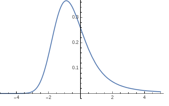
The function is unimodal: increasing from to some and decreasing then (see e.g. [28], Theorem 2.7.6) and simulations give In particular, if and we have:
| (2.1) |
The tails of are extremely asymetric: exponentially decreasing to zero at and polynomially decreasing to zero at . More precisely, the function admits the following expansion at :
| (2.2) |
and the following equivalent at :
| (2.3) |
These expansions relies on the following results for Ai and its derivative Ai′ (see e.g. [25] p.14):
| (2.4) |
and
| (2.5) |
The expansions (2.2) and (2.3) then follow using (2.4) and (2.5) with .
We give a crucial lemma on the ratio which appears in the jump kernel of .
Lemma 2.1.
Let be fixed. The function is non-decreasing on .
Proof.
First recall that the Airy function is positive and decreasing on , and its derivative is non-decreasing on (see [25]). Using , we have:
Therefore we obtain:
where
It is easy to see that for and , we have and so that
To show that is positive, we still have to show that
To do so, we decompose:
On , Ai is positive and Ai’ negative, so that we easily see that the first two terms are positive (remember that is negative), and just have to show that the last term is also positive. Since is negative and positive, we have and we are reduced to show that:
| (2.6) |
We thus introduce, for any constant :
Since we have for all :
so that we only have to prove that is positive for large where we can use the asymptotics (2.4) and (2.5) to get:
which is indeed positive for any . ∎
We end this section with results about integrals involving the function which will help us to control the expectation and variance of in Section 3.1 and to approximate the predictable compensator (Lemma 3.7) in Section 3.2. For we define:
| (2.7) |
| (2.8) |
and
| (2.9) |
We will also have to restrict ourselves to jumps smaller than , which prompts us to define:
| (2.10) |
Lemma 2.2.
There exists , , and such that for all we have:
Proof.
We begin by showing that for a constant and large enough we have:
| (2.11) |
From the asymptotic expansion (2.2) for there exists such that for all and we have:
| (2.12) |
In particular for :
with
We perform the change of variables in both integrals and get:
and
which gives the upper bound (2.11) for .
We now prove the lower bound
| (2.13) |
for a constant and large enough. The proof is similar to the previous one, we use (2.2) and get the existence of such that for all :
so that for all we have:
We perform the same change of variables as before and get:
which gives the lower bound (2.13) for large enough.
The proof of the result for is similar, we show that
for a constant and large enough. We first use (2.12) to get the existence of such that for all and we have:
which gives the result. The proof for is exactly the same, and we do not detail it.
The proof of the claim for is similar: thanks to (2.2) we find such that for all and we have:
so that for all we have:
where we take to be even larger than before, if necessary to make the terms in and small. We can conclude since goes to infinity when goes to infinity. ∎
2.2 Background on
We now turn to the process : we first give a construction of the process in terms of a Poisson point process that we will widely use all along the article. We have the following proposition (a sketch of proof is given for in [8], and a rigorous proof is given for general parameters in [26]):
Proposition 2.3.
There exists a Poisson point process over with (infinite) measure intensity such that for all :
| (2.14) |
where are the atoms of the process .
We finish with a last claim on , and refer to [21], Chapters 4 and 20 for definitions.
Proposition 2.4.
For all the process is a non-explosive, aperiodic, irreducible Feller process.
Proof.
Irreducibility and aperiodicity are both consequences of the fact that the support of the jump measure is the whole space since the density with respect to Lebesgue measure of the jump-measure is everywhere positive.
The non-explosivity is a consequence of the fact that for all and we have
To see this we decompose
| (2.15) |
For the first integral, we notice that for fixed , for and , by compactness, the ratio is bounded by a constant only depending on and so that
where is also only depending on and .
Remark.
For the number of jumps on a finite time interval is almost surely finite: indeed in this case for all and we have
which prevents the accumulation of small jumps (notice that this is not true for where there is indeed an accumulation).
3 The case
We begin with an overview of the proof of Theorem 1.1: our strategy is to introduce the predictable compensator of (defined in (3.10)) and to approximate by its compensator. The compensator has the advantage of being easier to work with than the process and we will see (Lemma 3.7) that it satisfies an equation close to
whose solution is . This is close to a "differential equation method" (see e.g. [27]) but the non-homogeneity in both time and space as well as the accumulation of small jumps prevents us from applying an existing theorem (as far as we know). The approximation relies on asymptotics on the function and we first need to show that for small enough, almost surely for large (Proposition 3.1) in order to use these asymptotics. This is the aim of Section 3.1 where we show this crude lower bound.
3.1 is larger than
In this section we study the process for but we will just write instead. We work on a probability space that we note . The goal of this section is to prove the following:
Proposition 3.1.
For small enough, almost surely, we have for all large enough.
Our strategy is to prove that for small enough (we will see later what we call by " small enough"):
so that, almost surely, for large enough, is larger than and Proposition 3.1 will follow since is increasing (taking instead of for example).
We first start with an easy but useful result: if follows a Poisson distribution of parameter , then for every , we have:
| (3.1) |
(this result is far from being optimal and exponential bounds can be obtained). This is a mere consequence of Markov’s inequality together with the fact that the fourth centered moment of a Poisson distribution of parameter is :
We first prove that tends to infinity when goes to infinity, which will be the "lauching point" to prove Proposition 3.1.
Lemma 3.2.
For any , there exists a constant and there exists such that for all we have:
Proof.
On the event we have for all :
where are the atoms of the Poisson point process whose intensity is on . For we thus have so that if we take , inequality (2.1) gives:
On we thus have:
Since are the atoms of , the random variable follows a Poisson distribution of parameter with and we conclude with (3.1). ∎
As an immediate corollary tends to infinity almost surely, and we prove now that is almost surely asymptotically larger than . We define:
| (3.2) |
Remark.
We have the following inequalities:
We introduce:
(with the convention ) the first time over the diagonal after time . We decompose according whether or not:
| (3.3) |
Lemma 3.3.
There exists a constant such that, for all large enough:
Proof.
To avoid making the notations more cumbersome in this proof we write and instead of and .
For we note Lemma 3.2 shows that for all , there exists such that for all large enough we have
We immediately deduce that for all there exists such that for all large enough:
so that to prove the lemma we can focus on
We now want to deal with the last term in (3.3), notice that we have not yet used the " small enough hypothesis" and we will need it in the following.
Lemma 3.4.
For every , the function is strictly positive in the neigbourhood of .
Proof.
We thus set small enough such that
| (3.4) |
For such we have the following:
Lemma 3.5.
There exists a constant such that, for all large enough we have:
Proof.
In this proof again we note and instead of and .
Thanks to Lemma 2.2, we find such that for all we have
| (3.5) |
For we define
Since on , there exists such that . Moreover, on , so that since is increasing we have for all :
We deduce the following inequality on :
We want to get rid of the terms in the indicator function, since they prevent us from calculating the expectation and variance. We prove that on , for large enough, for all and :
| (3.6) |
Indeed if , since is increasing we have , so that and we then have two possibilities:
- •
- •
We deduce that on :
which gives the inclusion:
| (3.7) |
We now compute the expectation and variance of using Campbell’s formula (see e.g. [16]) and (3.5), and get that for all :
so that (3.4) yields:
| (3.8) |
Thanks to (3.5) and Campbell’s formula, we have for all :
| (3.9) |
with . We conclude as follows with (3.7), (3.8) and (3.9):
with . ∎
3.2 Proof of Theorem 1.1
In this section we prove Theorem 1.1 which states the almost sure convergence of to when goes to infinity. From the previous section, for small enough, we have almost surely for large enough, which implies and which allows us to use the asymptotics of the function to approximate our processes. It will be easier to work with the predictable compensator of our process defined for by:
| (3.10) |
With this definition
is a martingale (see e.g. [12], Chapter 4). We first show that converges almost surely, to justify our work on the compensator. We first set small enough such that (3.1) holds.
Lemma 3.6.
The martingale converges almost surely when , and its limit is almost surely finite.
Proof.
To prove the lemma, we compute the quadratic variation of and show that is almost surely finite. For , we have ([12], Chapter 4) :
| (3.11) |
We know that almost surely there exists such that for all , . Thanks to Lemma 2.2 we thus have for all :
where the last line is a consequence of for so that the integral converges. ∎
This lemma enables us to approximate our process by its predictable compensator . The goal of the next lemma is to get a sort of "differential equation" for .
Lemma 3.7.
There exists a constant , and there exists with almost surely such that for all we have:
Before moving on to the proof of this lemma, let us explain how we will use it later. Lemma 3.7 approximates the compensator by the integral . We will write and approximate by its limit. This will give us two inequalities for , in the form of a differential equation (Equations (3.2) and (3.2)) and we will use results on comparisons of under and over-solutions of differentiable equations to get a result (we will just need to be careful about differentiability since our process is not differentiable everywhere). We first give a quick proof of Lemma 3.7.
Proof.
With the notations of Lemma 2.2 we have that for all :
| (3.12) |
Almost surely there exists such that for all we have . In particular, thanks to Lemma 2.2 we get that almost surely there exists so that for all we have:
and
so that for all large enough:
since for all . We get the lower bound in the same way. ∎
As our strategy is to compare solutions of differential equations, we need a starting point of comparison, which is the object of the following lemma.
Proposition 3.8.
For every , almost surely,
Proof.
The proof is a consequence of Lemma 3.7, the little subtlety is that we need to have both inequalities simultaneously. We let and define
Since converges almost surely to a finite limit , we only need to show that
We note and take . There exists such that for all we have
| (3.13) |
Since , taking larger if necessary, we can assume that for all , we have
| (3.14) |
Using Lemma 3.7, (3.13) and (3.14) we get for all :
Since is finite on and the logarithmic term tends to infinity when , we get a contradiction, and has to be a null event. With the exact same reasoning we get that almost surely
As we said before, we need to get both simultaneously. Since only has positive jumps, it cannot alternate over the line and under the line . ∎
From this point all the remaining work is deterministic, we fix (but will forget it in our notations) such that with and where is such that Proposition 3.1, Lemma 3.6 and Proposition 3.8 hold. From Lemma 3.6 converges to when goes to infinity and we thus take and such that for all :
| (3.15) |
We focus on:
which approximates by Lemma 3.7. Writing and using , we get:
The function is left and right-differentiable almost everywhere and for all we have:
and
Since is such that (3.15) holds, using Lemma 3.7, we get:
| (3.16) |
and
| (3.17) |
and replacing with we get the same inequalities for . The function is thus an under-solution of the equation
and an over-solution of the equation
Exact solutions of these equations are not explicit, but it is not difficult to find an over-solution for and an under-solution for . We will then compare it with our function , taking care since is not differentiable. We define, for :
| (3.18) |
and
| (3.19) |
It is not difficult to check that is an over-solution of and an under-solution for , for example:
since we can take large enough so that is positive. We want to compare with both and , we first must have a starting point. We notice that and that:
so that for our starting point, we need to have and which means:
which is exactly Proposition 3.8 and we can thus assume that is such that:
| (3.20) |
From this starting point, we use a standard method for comparing solutions with under and over-solutions of differential equations, we just have to be careful since is not differentiable. Recall that is an under-solution of and and over-solution of . In the same time, is an over-solution of and and under-solution of . The following proposition shows that stays between and in the future of :
Proposition 3.9.
For all , we have:
| (3.21) |
We recognize on the left-hand side and on the right-hand side.
Proof.
We show both inequalities separately, beginning with , since it is a bit easier.
Proof of the left-hand side inequality
Thanks to Proposition 3.8, we have We first notice that this comparison still holds in a closed future of since is non-decreasing and continuous.
We introduce:
(with the convention ). By contradiction, let us assume that . From the previous paragraph, we have . We first notice that
We have two possibilities: either or .
-
•
If :
Then for small, we have:
since . But this contradicts the definition of as an infimum.
-
•
If : for this case, notice that the function
is decreasing in . In particular we have:
Since and we deduce:
We conclude, in a similar way to the first case: for small we have:
since . This is again a contradiction and concludes the first part of the proof.
Proof of the right-hand side inequality
We want to show that for all . From Proposition 3.8 we know that . We use the same method as before and prove first that the inequality is still true in a closed future of . This is the only additional difficulty of this case since we cannot use the growth argument for we used in the first case. We solve it using a "contraction" property for the function . For sake of clarity we note . With this notation, for we have:
for a constant We have and so that from the contraction property, we have for :
which gives for small :
The rest of the proof is exactly the same as in the first case and is left to the reader. ∎
We can finally conclude the proof of Theorem 1.1:
4 The case
In this section we prove Theorem 1.2 which states the convergence of to a stationary law when goes to infinity, and gives tail inequalities for the stationary law. As in the previous section, we forget the in the notation and just write . We use a different strategy to the one used in the case based on the fact that when the process is a homogeneous Markov process. We use a Foster-Lyapunov criterion for Markov processes ([21], Theorem 20.3.2): if we denote the extended generator of the process , we will find a Lyapunov function such that
| (4.1) |
where , and is a petite set (see e.g. [20] for a definition).
4.1 Extended generator
Lemma 4.1.
The process is a non-explosive, irreducible, aperiodic, homogeneous Markov process, with extended generator
and whose domain contains functions of the form for and some .
Proof.
Non-explosivity, irreducibility and aperiodicity have already been discussed in Proposition 2.4. Let be the family of generators associated to the (inhomogeneous) process . We have, for and :
| (4.2) |
Then, if is the generator of , we have for and :
Let and for . Applying the previous equality to , we get:
By evaluating this equation in we therefore have:
We thus deduce that:
so that if , we have:
| (4.3) |
Notice that we did not talk about domain in this proof, we will not describe it entirely but we need to make sure that the function we will use in (4.1) belongs to . For this we need
to be a local martingale. The difficulty is about the integrability condition and this follows from the fact that for all and
We do not detail here why functions of the form for do check this condition, as it would be redundant with what follows, but hopefully it will become clear after the calculations in the next section.∎
4.2 Proof of Theorem 1.2
This is the technical part of the proof. We set
with
Thanks to the asymptotics (2.2) and (2.3) on , we let be such that for all :
| (4.4) |
and for all :
| (4.5) |
We then take (we will see in the proof the conditions required for ) and finally define and . We prove the following:
Lemma 4.2.
Let defined above. There exists such that for all we have:
With this lemma, Theorem 1.2 follows from Lyapunov criterion for homogeneous Markov processes ([21], Theorem 5.1) and we also get the tail inequalities for the stationary law.
Proof of Theorem 1.2:.
From Lemma 4.2 we have
with . To conclude with (4.1) we need the set to be petite. It is a consequence that all compact sets are petite sets for the process (see e.g [24], Theorems 5.1 and 7.1). Since is a non-explosive, irreducible, aperiodic process, we can apply Foster-Lyapunov criterion ([20], Theorem 5.1) and get that converges to a stationary law when .
Finally, the tail inequalities for are a consequence of inequality (4.1) with with and some . We integrate this inequality with respect to the probability measure and use that if then . We get:
Since is a probability measure, we deduce that for all and for some :
In particular, both and are finite and we finish the proof using Markov’s inequality. ∎
We still need to prove Lemma 4.2, which is quite heavy and technical.
Proof.
We decompose the tasks whether is in our petite set or not.
Case :
In this case the asymptotics (4.5) give that for all :
| (4.6) |
Then, from the expression (4.3) of and the choice of , we have for all :
Using (4.6) we hence get:
where we used that so that . We finally use the two easy following facts: if
where is the Gamma function, defined for Using these with , we deduce that:
Taking large enough we thus have for all which concludes in this case.
Case :
This case is quite similar to the previous one, we just have to be careful since the derivation term in the generator expression is positive and we will need to find negative contribution in the integrals. For we have:
We first get rid of the part of the integral where since is negative in this case so the integral between and is negative so that:
| (4.7) |
To find a negative contribution in (4.7), we decompose our integral, whether or not (recall ). In the first case it is easy to see that is negative and we must therefore lower bound
Since , from (4.4) we get
Then notice that if we have so that
We thus have:
| (4.8) |
We finally have to deal with the part of the integral in (4.7). Since , (4.4) gives:
Then implies so that from (4.5) we get:
We hence get:
| (4.9) |
where we used that for and we have:
with and .
We finally put (4.7), (4.8) and (4.9) together to get that for all
Since , we easily see that it is possible to choose such that for all we have
Case :
We want to show that for all , we have for a constant independent of . This is a mere consequence of the continuity of the application
on the compact set . Indeed for , we have:
so that the continuity is a consequence of clasical results of continuity for parameter-dependent integral (the domination follows from our choice of ). And for we have:
which gives us both the continuity on (from our choice of and and the continuity in .∎
Remark.
The proof of Theorem 1.2 gives more information on the tail of . Indeed we easily see that for all . From the expansion of , seems to be an optimal bound. The upper bound for the left side of the tail is a bit disappointing, and we could also expect . Optimizing our method could easily lead to but this is still less than
5 Applications on multiplicative coalescents
We give some applications of our results, especially Corollary 5.3 states the convergence of the scaling limit of the forest part of the frozen Erdős-Rényi graph with parameter to a stationary law. We also give a consequence on Aldous’ multiplicative coalescent. As mentioned in the introduction, in the critical window the process of the decreasing sizes of the frozen components renormalized by followed by the decreasing sizes of the standard components renormalized by in converge towards a process
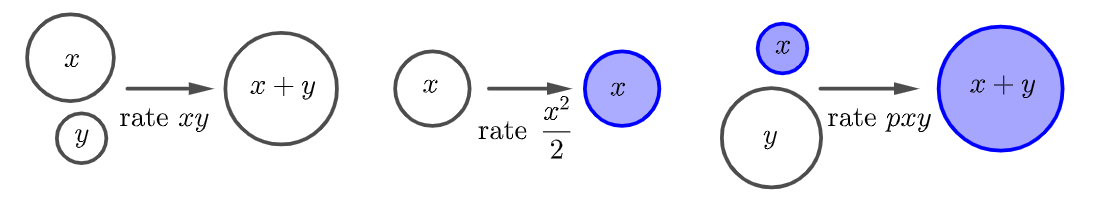
called the frozen multiplicative coalescent. This process has been introduced for in [8] and is generalized for in [26]. Just as the frozen graph is a modification of the classical Erdős-Rényi graph, the frozen multiplicative coalescent is a modification of Aldous’ standard multiplicative coalescent. For reminder the multiplicative coalescent is a process with values in , and intuitively, a pair of particles of mass and merges to a new particle of mass at rate . The general idea is to recover the dynamics of the sizes of the connected components of the Erdős-Rényi graph. The idea of the frozen multiplicative coalescent of parameter is the same: the particles of the frozen multiplicative coalescent at time are of two types: the frozen particles whose decreasing masses are in and the standard particles whose decreasing masses are in . Every pair of standard particles of mass and merges to a standard particle of mass at rate , a standard particle of mass freezes at rate and a standard particle of mass and a frozen particle of mass merges to a frozen particle of mass at rate .
We give some notations: for , we shall denote:
(notice that with these notations we have ). As we will need it later to state Corollary 5.2 notice that there exists an augmented multiplicative coalescent (see [6] for a construction) where the process is the scaling limit of components’ surplus in . This allows us to talk about the surplus of the multiplicative coalescent.
Our results also involves scaling limits of critical random forests, studied by Martin and Yeo in [19] so we recall their description from [8]: for and we note a uniform random forest with vertices and edges (be careful that there is no obvious coupling of for variying ). Inspired by the critical window, for we note
and the sequence of its component sizes in decreasing order renormalized by . We let be a stable Lévy process with index and only positive jumps, starting from and with Lévy measure , so that for the density of is , where for :
(see e.g. [3], Chapter VIII or [28]). For any , we define the process obtained by conditioning the process to be equal to at time (this is called a Lévy bridge and is a degenerated conditioning but still can be obtained with the help of transforms [3]). With these notations, Contat and Curien [8] proved that for every fixed the following convergence holds:
| (5.1) |
for the topology for any fixed .
Recall the notation (respectively ) the decreasing sizes of standard (respectively frozen) particles in . Equipped with these notations we have the following proposition for the law of standard particles in .
Proposition 5.1.
For every , for every , conditionally on the total frozen mass , the law of the sizes of the standard particles is the same as the law of , the law the jumps of the conditioned Lévy process .
In particular for , since the only discarded edges are the edges connecting two frozen vertices, the forest part of and coincide:
In the limit we get that the vector of the sizes of the standard particles is equal to the vector of the sizes of particles without surplus in the augmented multiplicative coalescent, which immediately gives the following corollary.
Corollary 5.2.
For every , the process of the total mass of the particles with surplus in has law , and, conditionally on it, the remaining particles are distributed as the jumps of the conditioned Lévy process .
We give a short proof of Proposition 5.1.
Proof of Proposition 5.1.
We know from [8] that for any and , conditionally on the number of edges of and on , the forest part of is a uniform random forest with
and
where is the total number of edges in . The number of vertices in is:
and the number of edges is:
where is the number of discarded edges in and is the analogue continous time version. It has been shown (see [8] for the case ) that in the critical window is of order . Combining this with the convergence of the total frozen mass, we get that for :
Combining this with the convergence of the frozen Erdős-Rényi to the frozen multiplicative coalescent, we get the desired proposition. ∎
We focus on : Proposition 5.1 states that conditionally on the size of the freezer, the particles without surplus are distributed as the jump of the conditioned Lévy process and Theorem 1.2 that converges to a stationary law when goes to . We immediately get the following proposition already announced in the introduction.
Corollary 5.3.
For all , we have the following convergence in distribution for the topology
where is a random variable with distribution .
As already explained in the introduction, the idea of this result is that the case the frozen components are completely stopped and the only way to increase the frozen mass is to create an intern cycle in a tree. As a consequence only "big" trees become frozen, whereas small trees stay without surplus. When a tree can freeze if it is connected with a unicycle, so that small trees have more probability to freeze, which prevents the existence of a stationary law for these components. Informally, since , for large the law of standard particles in is the law of a -stable Levy process with only positive jumps conditioned to be very negative a time (roughly equal to ). The jumps of such a process necessarily tends towards when goes to .
References
- [1] D. Achlioptas, R. M. D’Souza, and J. Spencer. Explosive percolation in random networks. Science, 323(5920):1453–1455, 2009.
- [2] D. Aldous. Brownian excursions, critical random graphs and the multiplicative coalescent. Ann. Probab., 25(2):812–854, 1997.
- [3] Jean Bertoin. Lévy processes, volume 121 of Camb. Tracts Math. Cambridge: Cambridge Univ. Press, 1998.
- [4] B. Bollobás. The evolution of random graphs. Trans. Am. Math. Soc., 286:257–274, 1984.
- [5] B. Bollobàs, S. Janson, and O. Riordan. The phase transition in inhomogeneous random graphs. Random Struct. Algorithms, 31(1):3–122, 2007.
- [6] N. Broutin and J.F. Marckert. A new encoding of coalescent processes: applications to the additive and multiplicative cases. Probab. Theory Relat. Fields, 166(1-2):515–552, 2016.
- [7] R. Cerf and N. Forien. Some toy models of self-organized criticality in percolation. ALEA, Lat. Am. J. Probab. Math. Stat., 19(1):367–416, 2022.
- [8] A. Contat and N. Curien. Parking on Cayley trees and frozen Erdős-Rényi. Ann. Probab., 51(6):1993–2055, 2023.
- [9] P. Erdős and A. Rényi. On random graphs. I. Publ. Math. Debr., 6:290–297, 1959.
- [10] E. N. Gilbert. Random graphs. Ann. Math. Stat., 30:1141–1144, 1959.
- [11] N. Ikeda and S. Watanabe. Stochastic differential equations and diffusion processes., volume 24 of North-Holland Math. Libr. Amsterdam etc.: North-Holland; Tokyo: Kodansha Ltd., 2nd ed. edition, 1989.
- [12] M. Jacobsen. Point process theory and applications. Marked point and picewise deterministic processes. Probab. Appl. Boston: Birkhäuser, 2006.
- [13] J. Jacod and A. N. Shiryaev. Limit theorems for stochastic processes., volume 288 of Grundlehren Math. Wiss. Berlin: Springer, 2nd ed. edition, 2003.
- [14] O. Kallenberg. Foundations of modern probability. Probab. Appl. New York, NY: Springer, 2nd ed. edition, 2002.
- [15] P. Krapivsky. Simple evolving random graphs. 2023.
- [16] G. Last and M. Penrose. Lectures on the Poisson process, volume 7 of IMS Textb. Cambridge: Cambridge University Press, 2018.
- [17] T. Łuczak. Component behavior near the critical point of the random graph process. Random Struct. Algorithms, 1(3):287–310, 1990.
- [18] T. Łuczak, B. Pittel, and J. C. Wierman. The structure of a random graph at the point of the phase transition. Trans. Am. Math. Soc., 341(2):721–748, 1994.
- [19] J. B. Martin and D. Yeo. Critical random forests. ALEA, Lat. Am. J. Probab. Math. Stat., 15(2):913–960, 2018.
- [20] S. Meyn and R. L. Tweedie. Stability of Markovian processes. III: Foster-Lyapunov criteria for continuous-time processes. Adv. Appl. Probab., 25(3):518–548, 1993.
- [21] S. Meyn and R. L. Tweedie. Markov chains and stochastic stability. Prologue by Peter W. Glynn. Camb. Math. Libr. Cambridge: Cambridge University Press, 2nd ed. edition, 2009.
- [22] B. Rath and B. Toth. Erdős-Renyi random graphs forest fires self-organized criticality. Electron. J. Probab., 14:1290–1327, 2009.
- [23] O. Riordan and L. Warnke. Achlioptas process phase transitions are continuous. Ann. Appl. Probab., 22(4):1450–1464, 2012.
- [24] R. L. Tweedie. Topological conditions enabling use of Harris methods in discrete and continuous time. Acta Appl. Math., 34(1-2):175–188, 1994.
- [25] O. Vallée and M. Soares. Airy functions and applications to physics. Hackensack, NJ: World Scientific, 2nd ed. edition, 2010.
- [26] V. Viau. Graphes d’Erdős-Rényi gelés. PhD thesis, Université Sorbonne Paris-Nord, (in preparation).
- [27] N. C. Wormald. The differential equation method for random graph processes and greedy algorithms. In Lectures on approximation and randomized algorithms. Proceedings of the Berlin-Poznań summer school, Antonin, Poland, September 1997, pages 73–155. Warsaw: Polish Scientific Publishers, 1999.
- [28] V. M. Zolotarev. One-dimensional stable distributions. Transl. from the Russian by H. H. McFaden, ed. by Ben Silver, volume 65 of Transl. Math. Monogr. American Mathematical Society (AMS), Providence, RI, 1986.