A Distributed Approach to Autonomous Intersection
Management via Multi-Agent Reinforcement Learning

Abstract

Autonomous intersection management (AIM) poses significant challenges due to the intricate nature of real-world traffic scenarios and the need for a highly expensive centralised server in charge of simultaneously controlling all the vehicles. This study addresses such issues by proposing a novel distributed approach to AIM utilizing multi-agent reinforcement learning (MARL). We show that by leveraging the 3D surround view technology for advanced assistance systems, autonomous vehicles can accurately navigate intersection scenarios without needing any centralised controller. The contributions of this paper thus include a MARL-based algorithm for the autonomous management of a 4-way intersection and also the introduction of a new strategy called prioritised scenario replay for improved training efficacy. We validate our approach as an innovative alternative to conventional centralised AIM techniques, ensuring the full reproducibility of our results. Specifically, experiments conducted in virtual environments using the SMARTS platform highlight its superiority over benchmarks across various metrics.

1 Introduction

Connected autonomous vehicles (CAVs) [1] represent a groundbreaking advancement in transportation: with the potential to revolutionize mobility, CAVs are poised to redefine how we commute, park, travel, transport and interact with our urban environments [2, 3]. Equipped with advanced sensors and artificial intelligence systems [4], CAVs can navigate roads with precision, mitigating the risk of accidents caused by human error [5, 6]. This enhanced safety feature not only saves lives but also instills confidence in passengers, making mobility more accessible and inclusive for individuals with disabilities or vulnerabilities [7, 8, 9]. On a societal level, the advantages of CAVs extend far beyond individual convenience. By optimizing traffic flow and minimizing congestion, CAVs have the potential to alleviate the strain on highways [10], reducing travel times and improving overall efficiency and stability [11]. Such a traffic management not only benefits commuters but also enhances the productivity of cities and supports economic growth [12, 13]. In addition, CAVs hold the promise of environmental sustainability. With the integration of electric and hybrid propulsion systems, CAVs can significantly reduce greenhouse gas emissions [14, 15] and combat climate change contributing to a cleaner, greener connected future [16].

Lately, significant strides in the development of CAVs have been made, largely attributed to the utilization of multi-agent reinforcement learning (MARL) [17] within the framework of smart mobility, showing promise in addressing autonomous intersection management (AIM) [18]. As it is widely believed that the resolution of AIM is pivotal to overcome in order to advance the adoption of CAVs, this control problem constitutes the primary focus for our study.

A vast literature exists on AIM. The research in this field spans multiple fronts, each leveraging distinct methodologies to address the challenges of optimizing traffic flow and ensuring safety in dynamic urban environments. By employing reinforcement learning (RL), AIM systems can effectively learn and adapt intersection control strategies in response to changing traffic conditions [19, 20]. These systems typically comprise priority assignment models, intersection control model learning, and safe brake control mechanisms. Experimental simulations demonstrate the superiority of RL-inspired AIM approaches over traditional methods, showcasing enhanced efficiency and safety. Graph neural networks (GNNs) have also garnered attention for their potential in AIM [21, 22]. Leveraging RL algorithms, GNNs optimize traffic flow at intersections by jointly planning for multiple vehicles. These models encode scene representations efficiently, providing individual outputs for all involved vehicles. Game theory serves then as a foundational framework for MARL approaches in AIM. Indeed, game-theoretic models facilitate safe and adaptive decision-making for CAVs at intersections [23, 24]. By considering the diverse behaviors of interacting vehicles, these algorithms ensure flexibility and adaptability, thus enhancing autonomous vehicle performances in challenging scenarios. Finally, recursive neural networks (RNNs) integrated in the MARL framework represent an interesting approach in AIM research, with the objective of learning complex traffic dynamics and optimizing vehicle speed control [25].

Despite the theoretical advancements in AIM techniques, their implementation still faces important challenges. The main obstacle is represented by the need for a highly expensive centralised server which has to be positioned in the proximity of the intersection, in order to simultaneously control all the vehicles. Moreover, the vehicles should continuously send their local information to this centralised controller, which will then gather and elaborate the data coming from all the road users, before sending back to each vehicle a velocity or acceleration command. Given the complexity and high demands of this technological framework, the integration of AIM devices into existing transportation infrastructures still requires many years of extensive research and testing. In this direction, we devise an alternative distributed approach based on the 3D surround view technology for advanced assistance systems [26]. As demonstrated in the sequel, such a method allows the reconstruction of a 360^∘ scene centered around each CAV, which is useful to recover the information required for each agent involved in the proposed MARL-based technique. This, in turn, grants to effectively carry out AIM in a decentralised fashion, exploiting sensors that are currently available on the market, without the need for the centralised infrastructure described in the previous lines.

More precisely, the contributions of this paper are multiple.

• As mentioned above, we offer a new distributed strategy that represents a competitive and realistic alternative to the classical centralised AIM techniques.

• Relying on self-play [27] and drawing inspiration from prioritised experience replay [28] to improve training efficacy, we develop a MARL-based algorithm capable of tackling and solving a 4-way intersection by means of the SMARTS platform [29].

• Our strategy outperforms a number of well-established benchmarks, which typically leverage traffic light regulation in function of travel time, waiting time and average speed.

• Last but not least, we guarantee full reproducibility of the code that is used for the generation of the virtual experiments shown in this manuscript.

The remainder of this paper unfolds as follows. The preliminaries for this study are yielded in Section 2; whereas, Section 3 provides the core of our contribution, namely the multi-agent decentralised dueling double deep q-networks algorithm with prioritised scenario replay (MAD4QN-PS). This innovative method is then tested and validated through several virtual experiments, as illustrated in Section 4. Finally, Section 5 draws the conclusions for the present investigation, proposing future developments.

Notation: The sets of natural and positive (zero included) real numbers are denoted by $\mathbb{N}$ and $\mathbb{R}_{0}^{+}$, respectively. Given a random variable (r.v.) $Y$, its probability mass function is denoted by $P[Y=y]$, whereas $P[Y=y\leavevmode\nobreak\ |\leavevmode\nobreak\ Z=z]$ indicates the probability mass function of $Y$ conditioned to the observation of a r.v. $Z$. Moreover, the expected value of a r.v. $Y$ is denoted by $\mathbb{E}[Y]$.

2 Theoretical background

2.1 Basic notions of reinforcement learning

RL is a machine learning paradigm in which an agent learns to solve a task by iteratively interacting with its environment. Solving the task means maximising the cumulative rewards obtained over time. A generic RL problem is formalised by the concept of Markov decision process (MDP) [30], which is a tuple composed by five elements: ${\left\langle\mathcal{S},\mathcal{A},\mathcal{P},\mathcal{R},\gamma\right\rangle}$. $\mathcal{S}$ and $\mathcal{A}$ are two generic sets, representing the state and action space respectively. ${\mathcal{P}\left(s,a,s^{\prime}\right)=P\left[S_{t+1}=s^{\prime}\mid S_{t}=s,A_{t}=a\right]}$ is the state transition probability function, in charge of updating the environment to a new state $s^{\prime}\in\mathcal{S}$ at each step, based on the previous state $s\in\mathcal{S}$ and the action $a\in\mathcal{A}$ performed by the agent. Moreover, the reward function $\mathcal{R}(s,a,s^{\prime}):\mathcal{S}\times\mathcal{A}\times\mathcal{S}\rightarrow\mathbb{R}$ is used to measure the quality of each transition, while $\gamma\in[0,1)$ denotes a discount factor, used to compute the cumulative reward at time $t$, i.e. the return $G_{t}=\sum_{k=0}^{\infty}\gamma^{k}r_{t+k+1}$. The agent decides which action to take at each iteration exploiting its policy, a function that maps any state to the probability of selecting each possible action:

$$\pi(a|s)=P[A_{t}=a\mid S_{t}=s],\hskip 8.5359pt\forall a\in\mathcal{A}.$$ (1)

Solving a RL problem means finding an optimal policy $\pi^{*}$. One criterion that is usually adopted to find $\pi^{*}$ consists in the maximization of the state-action value function $Q_{\pi}(s,a)$, i.e. the expected return starting from state $s\in\mathcal{S}$, taking action $a\in\mathcal{A}$, and thereafter following policy $\pi$:

$$Q_{\pi}(s,a)=\mathbb{E}_{\pi}\left[G_{t}\mid S_{t}=s,A_{t}=a\right].$$ (2)

Consequently, given the state-action value function, the optimal policy is defined as $\pi^{*}=\text{arg}\max_{\pi}Q_{\pi}(s,a)$. There is therefore an inherent relation between $\pi^{*}$ and the optimal state-action value function.

Finally, two other important quantities which will be used in the proceeding of this article are the state value function and the advantage function. The former is defined as the expected return starting from state $s\in\mathcal{S}$ and then following policy $\pi$:

$$V_{\pi}(s)=\mathbb{E}_{\pi}\left[G_{t}\mid S_{t}=s\right].$$ (3)

The latter instead is used to give a relative measure of importance to each action for a particular state, and it is defined starting from $Q_{\pi}(s,a)$ and $V_{\pi}(s)$:

$$A_{\pi}(s,a)=Q_{\pi}(s,a)-V_{\pi}(s).$$ (4)

2.2 Q-Learning and Deep Q-Networks

To compute the optimal state-action value function we could theoretically exploit the recursive Bellman Optimality Equation [31]:

$$Q^{*}(s,a)=\mathbb{E}\left[r_{t+1}+\gamma\max_{a^{\prime}}Q^{*}(S_{t+1},a^{\prime})\mid S_{t}=s,A_{t}=a\right],$$ (5)

however due to the curse of dimensionality and the need for perfect statistical information to compute the closed-form solution, it is necessary to resort to iterative learning strategies even to solve simple RL problems. The most common algorithm used in literature is Q-Learning [32], where the state-action value function is represented by a table, which is iteratively updated at each step through an approximation of (5):

$$Q_{t+1}(s_{t},a_{t})\leftarrow\hskip 2.84544ptQ_{t}(s_{t},a_{t})+\alpha(r_{t+1}+\gamma\max_{a^{\prime}}Q_{t}(s_{t+1},a^{\prime})-Q_{t}(s_{t},a_{t})),$$ (6)

where $\alpha>0$ is called the step-size parameter. The policy derived from the state-action value function is usually the $\varepsilon$-greedy policy, suitable to balance the trade-off between exploration and exploitation. [30]:

$$\pi(a|s)=\begin{cases}\text{arg}\max_{a}Q(s,a)\hskip 14.22636pt&\text{with probability $1-\varepsilon$}\\ \text{random action }a\in\mathcal{A}&\text{with probability $\varepsilon$}\end{cases}$$ (7)

Tabular Q-Learning works well for simple tasks, but the problem rapidly becomes intractable when the state space becomes very large or even continuous. For this reason state-of-the-art RL algorithms employ function approximators, such as neural networks (NNs), to solve realistic and complex problems. One of the first yet more used deep RL algorithms is Deep Q-Networks [33], which approximates the state-action value function through a NN, $Q(s,a;\theta)$. A replay memory is used to store the transition tuples $(s,a,r,s^{\prime})$. Finally, the parameters $\theta$ of the Q-Network are optimised by sampling batches $\mathcal{B}$ of transitions from the replay memory and minimizing a mean squared error loss derived from (6):

$$\mathcal{L}(\theta)=\cfrac{1}{|\mathcal{B}|}\sum_{i\in\mathcal{B}}[(r_{i}+\gamma\max_{a^{\prime}}Q(s_{i}^{\prime},a^{\prime};\bar{\theta})-Q(s_{i},a_{i};\theta))^{2}],$$ (8)

where $\bar{\theta}$ represent the parameters of a target network, which are periodically duplicated from $\theta$ and maintained unchanged for a predefined number of iterations.

2.3 Multi-agent reinforcement learning

MARL expands upon traditional RL by incorporating multiple agents, each making decisions in an environment where their actions influence both the immediate rewards and the observations of other agents. In its most general definition, a MARL problem is formalised as a partially observable stochastic game (POSG), in which each agent has its own action space and reward function. Moreover, the partial observability derives from the fact that the agents do not perceive the global state, but just local observations, which carry incomplete information about the environment [34].

MARL algorithms can be categorised depending on the type of information available to the agents during training and execution: in centralised training and execution (CTCE), the learning of the policies as well as the policies themselves use some type of structure that is centrally shared between the agents. On the other hand, in decentralised training and execution (DTDE), the agents are fully independent and do not rely on centrally shared mechanisms. Finally, the centralised training and decentralised execution paradigm (CTDE) is in between the first two, exploiting centralised training to learn the policies, while the execution of the policies themselves is designed to be decentralised [35].

3 Multi-Agent Decentralised Dueling Double Deep Q-Networks with Prioritized Scenario replay

In this section we present our novel method based on MARL, called Multi-Agent Decentralised Dueling Double Deep Q-Networks with Prioritized Scenario replay (MAD4QN-PS). We begin by detailing how the system is modelled, and then we describe the original learning procedure that we implement in order to train agents through self-play [27]. Finally, we shall introduce the prioritised scenario replay pipeline that is implemented to speed up training.

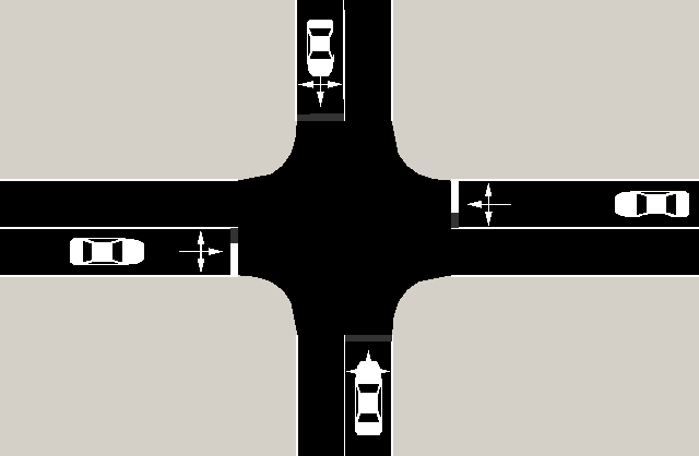
Figure 1: Visual representation of the 4-way 1-lane intersection environment considered for the experiments (image created through SUMO simulator [36]).

3.1 System modelling and design

The environment in which the agents live consists of a 4-way 1-lane intersection, with three different turning intentions available to each vehicle, as shown in Figure 1.

Recalling Section 2.3, we formalize the problem as a POSG, which can be seen as a multi-agent extension to MDPs. For this reason, we shall define for each agent the observation space, the action space and the reward function.

The information retrieved by each vehicle at every time step consists of a local RGB bird-eye view image with the vehicle at the center. As already discussed in Section 1, this type of data is already recoverable from sensors with modern technology, thus making such a configuration extremely interesting from an application point of view. Moreover, the final observation passed to the agent is represented by a stack of $n\in\mathbb{N}$ consecutive frames, thus allowing the algorithm to capture temporal dependencies and understand how the environment is changing over time.

The action space of each agent instead is discrete and it contains $m\in\mathbb{N}$ velocity commands. This choice has been made because the purpose of our algorithm is not to learn the basic skills required for driving, such as keeping the lane and following a trajectory, but it is instead choosing how to behave in traffic conditions and when to interact with other vehicles present in the environment. Moreover, a similar high-level perspective has also been implemented in other works, related to the centralised AIM paradigm [21, 22, 25].

Finally, for what concerns the reward function, we need to take into consideration the fact that each agent is trying to solve a multi-objective problem. Indeed the main goal of each vehicle is crossing the intersection and reaching the end of the scenario. In the meantime, a vehicle is also required not to collide with the others, by travelling as smoothly as possible. In order to fulfill all these objectives we design a reward signal composed by different terms:

$$r=\begin{cases}+x\hskip 24.18501pt&\text{if}\hskip 8.5359pt||x||>0,\\ -k&\text{if vehicle not moving,}\\ -10\cdot k&\text{if a collision occurs,}\\ +10\cdot k&\text{if scenario completed,}\end{cases}$$ (9)

where $x\in\mathbb{R}_{0}^{+}$ is the distance travelled in meters from the previous time step and $k\in\mathbb{N}$ is a hyperparameter used to weight the importance of the last three components of the reward function with respect to the first one.

3.2 Learning Strategy

The starting point for our learning strategy is the algorithm Deep Q-Networks, already presented in Section 2.2. This algorithm is then slightly modified by considering the Double DQN scheme and also the Dueling architecture, which will be briefly introduced in the sequel.

The idea of Double DQN [37] is originated by the fact that Q-Learning, and consequently also DQN, are known to overestimate state-action values under certain conditions. This is due to the max operation (see in (6) and (8)) performed to compute the temporal difference target. To mitigate this effect, the idea is to decouple the action selection and evaluation steps by using two different networks. We thus exploit the online network in the action selection step, while we keep using the target network for evaluation. This leads to the following modification of the loss function:

$$\mathcal{L}(\theta)=\cfrac{1}{|\mathcal{B}|}\sum_{i\in\mathcal{B}}[(r_{i}+\gamma Q(s_{i}^{\prime},\text{arg}\max_{a^{\prime}}Q(s_{i}^{\prime},a^{\prime};\theta);\bar{\theta})-Q(s_{i},a_{i};\theta))^{2}].$$ (10)

Dueling DQN [38] instead introduces a modification in the NN architecture. Instead of having a unique final layer that outputs the Q-value for each possible action, we split it in two, with the first layer in charge of estimating the state value function (3) and the second layer used for evaluating the advantage function (4). These two quantities are then combined in the following way to produce an estimate of the state-action value function:

$$Q(s,a;\theta,\alpha,\beta)=V(s;\theta,\alpha)+(A(s,a;\theta,\beta)-\cfrac{1}{|\mathcal{A}|}\sum_{a^{\prime}}A(s,a^{\prime};\theta,\beta)),$$ (11)

where $\alpha$ and $\beta$ are the network parameters of the final layer, specific for the state-value function and advantage function respectively. Whereas, subtracting the term $\frac{1}{|\mathcal{A}|}\sum_{a^{\prime}}A(s,a^{\prime};\theta,\beta)$ is needed for stability reasons.

The final algorithm used for training is therefore a Multi-Agent version of Dueling Double DQN known as D3QN, with linearly-annealed $\varepsilon$-greedy policy for all the agents. In order to allow for decentralised execution while developing at the same time a smart training strategy, we consider an intermediate approach between the DTDE and the CTDE paradigms. In particular, we initialize and train three different D3QN agents, one for each turning intention, i.e. left, straight and right. In this way each vehicle can select which model to use at the beginning of its path, according just to its own turning intention.

This approach is extremely sample-efficient, because we keep the number of network parameters constant, regardless of the number of vehicles considered. Moreover, these shared parameters are optimised through the experiences generated by all the vehicles, leading to a more diverse set of trajectories for training. Indeed, each of the three models has its own replay buffer, which contains transitions shared from all the vehicles with the corresponding turning intention. The crucial insight that makes our strategy effective is the fact that the observations gathered from each vehicle are invariant with respect to the road in which the vehicle itself is positioned. This parameter and experience sharing approach renders the training procedure of the algorithm somehow centralised because trajectories coming from different vehicles are used to train the three D3QN agents. However, we remark that, once the models have been trained, the execution phase is completely decentralised, since each vehicle locally stores the three different models. Then, at the beginning of the scenario, each CAV selects the model to use based only on its own turning intention.

3.3 The prioritised scenario replay strategy

The agents are trained for a fixed number of iterations $N\in\mathbb{N}$, keeping the intersection busy in order to obtain meaningful transitions to learn from. In particular, at each episode we consider the most complicated situation in which there are four vehicles simultaneously crossing the intersection, one for each road and with random turning intention.

Every $E\in\mathbb{N}$ time steps we pause training and run an evaluation phase. During this period, the agents use a greedy policy to face all the possible scenarios described above. When the evaluation is completed, we use the inverse of the returns from all the scenarios to build a probability distribution, and in the following training window we sample the different scenarios according to such a distribution. In this way we allow the agents to learn more from the most complicated situations. We name this original training strategy prioritised scenario replay because of its conceptual similarity with the prioritised experience replay scheme [28], common in many RL algorithms. Algorithm 1 illustrates the proposed learning strategy in detail.

Algorithm 1 MAD4QN-PS

1:  Initialize three state-action value networks $Q_{i}$ with random parameters $\theta_{i}$, $i=1,2,3$

2:  Initialize three target state-action value networks $\bar{Q}_{i}$ with parameters $\bar{\theta}_{i}=\theta_{i}$, $i=1,2,3$

3:  Initialize three replay buffers $\mathcal{D}_{i}$, $i=1,2,3$

4:  Setup initial $\varepsilon$, decay factor $\varepsilon_{d}$, evaluation period $E$, target update period $\delta$, discount factor $\gamma$

5:  Uniformly initialize the scenarios probability distribution

6:  max_episode_steps $\leftarrow M$

7:  $n\leftarrow 0$

8:  while $n<N$ do

9:     episode_terminated $\leftarrow$ False

10:     Randomly reset the environment

11:     episode_steps $\leftarrow 0$

12:     while not episode_terminated do

13:        $V\leftarrow$ number of vehicles currently present in the simulation

14:        Assign each vehicle to one of the three agents, based on its turning intention

15:        Collect observations for each vehicle $o_{1}^{n},...,o_{V}^{n}$

16:        for all vehicles $v$ in $1,...,V$ do

17:           With probability $\varepsilon$ select a random action $a_{v}^{n}$

18:           Otherwise $a_{v}^{n}\leftarrow\text{arg}\max_{a}Q_{i}(o_{v}^{n},a;\theta_{i})$, where $i$ depends on the turning intention of  $v$

19:        end for

20:        Apply actions $a_{v}^{n}$ and collect observations $o_{v}^{n+1}$ and rewards $r_{v}^{n}$ for $v$ in $1,...,V$

21:        Store each transition in the corresponding replay buffer $\mathcal{D}_{i}$, $i=1,2,3$

22:        for all agents $i=1,2,3$ do

23:           Sample random batch of transitions $\mathcal{B}_{i}$ from replay buffer $\mathcal{D}_{i}$

24:           Update parameters $\theta_{i}$ by minimising the loss function:

$$\mathcal{L}(\theta_{i})=\cfrac{1}{|\mathcal{B}_{i}|}\sum_{b\in\mathcal{B}_{i}}[(r_{b}+\gamma\bar{Q}_{i}(o_{b}^{\prime},\text{arg}\max_{a^{\prime}}Q_{i}(o_{b}^{\prime},a^{\prime};\theta_{i});\bar{\theta_{i}})-Q_{i}(o_{b},a_{b};\theta_{i}))^{2}]$$

25:        end for

26:        $\varepsilon\leftarrow\varepsilon-\varepsilon_{d}$

27:        episode_steps $\leftarrow$ episode_steps + 1

28:        $n\leftarrow n+1$

29:        if $n$ % $\delta==0$ then

30:           Update target network parameters $\bar{\theta}_{i}=\theta_{i}$ for each agent $i=1,2,3$

31:        end if

32:        if $n$ % $E==0$ then

33:           Run evaluation phase and update the scenarios probability distribution as described in Section 3.3

34:        end if

35:        if a collision occurred or $V==0$ or episode_steps == max_episode_steps then

36:           episode_terminated $\leftarrow$ True

37:        end if

38:     end while

39:  end while

4 Experiments on virtual environments

In order to train and evaluate our algorithm we need a suitable simulation environment. For this project we have chosen the platform SMARTS [29], explicitly designed for MARL experiments for autonomous driving. SMARTS relies on the external provider SUMO (Simulation of Urban MObility) [36], which is a widely used microscopic traffic simulator, available under an open source license. For our setup, we have used SMARTS as a bridge between SUMO and the MARL framework, since it follows the standard Gymnasium APIs [39], widely used in the RL community.

To develop our code Python 3.8 was employed along with the version 1.4 of the Deep Learning library PyTorch [40]. Moreover, a NVIDIA TITAN Xp GPU was used to run our experiments.

As already mentioned in Section 3.1, we have built a 4-way 1-lane intersection scenario, with three different turning intentions available to the vehicles coming from each of the four ways. The simulation step has been fixed to 0.1$s$. Regarding the observation of each vehicle, we have stacked $n=3$ consecutive frames, each consisting of a RGB image of dimensions $48\times 48$ pixels. Whereas, the action space contains $m=2$ possible velocity commands, namely $0$ and $15$$m$/$s$. These references are then fed at each iteration to a speed controller, in charge of driving the vehicle until the subsequent time step. For what concerns the reward function (9), we have fixed its hyperparameter to $k=1$. Regarding the architecture of the NN used to approximate the state-action value function, we have considered a convolutional neural network (CNN), whose structural details are summarised in Table 1. Finally, the training hyperparameters of Algorithm 1 are reported in Table 2.

Table 1: CNN architecture

Layer	N. of Filters	Kernel Size	Stride	Activation Function	N. of Neurons
Convolutional	$32$	$8\times 8$	4	ReLU	/
Convolutional	$64$	$4\times 4$	2	ReLU	/
Convolutional	$64$	$3\times 3$	1	ReLU	/
Fully connected	/	/	/	ReLU	512
Fully connected (V)	/	/	/	Linear	1
Fully connected (A)	/	/	/	Linear	2

Table 2: Training hyperparameters

Hyperparameter	Symbol	Value	Hyperparameter	Symbol	Value
Training steps	$N$	$10^{6}$	Initial exploration rate	$\varepsilon$	$1$
Max episode steps	$M$	$10^{3}$	Exploration rate decay	$\varepsilon_{d}$	$10^{-6}$
Evaluation period	$E$	$5\cdot 10^{3}$	Buffer size	$|\mathcal{D}|$	$1.5\cdot 10^{5}$
Optimizer	/	RMSprop [41]	Discount factor	$\gamma$	$0.99$
Learning rate	$lr$	$10^{-4}$	Batch size	$|\mathcal{B}|$	$256$
Target update period	$\delta$	$10^{3}$

4.1 Baselines

In order to assess the quality of our algorithm, we benchmark it versus the following baselines :

• Random policy (RP) for all the vehicles, which helps confirm whether our algorithm is effectively learning meaningful patterns, as it demonstrates its ability to outperform random actions, which lack any deliberate learning process.

• Two symmetric (N/S & W/E) fixed-time traffic lights (FTTL) [22, 25], with different cycle lengths.

• Two symmetric (N/S & W/E) actuated traffic lights (ATL) [36], with different cycle lengths, which operate by transitioning to the next phase once they identify a pre-specified time gap between consecutive vehicles. In this way the allocation of green time across phases is optimised and the cycle duration is adjusted in accordance with changing traffic dynamics.

The parameters of the four traffic lights configurations are reported in Table 3.

Table 3: Traffic lights parameters

Traffic light	Red & Green	Yellow	Min. Duration	Max. Duration
FTTL1	$25s$	$5s$	/	/
FTTL2	$32s$	$8s$	/	/
ATL1	$25s$	$5s$	$10s$	$40s$
ATL2	$32s$	$8s$	$15s$	$50s$

As a final note, we emphasize that we do not have considered any RL-based centralised AIM approach as baseline because the purpose of our method is to propose a more realistic and feasible alternative to them, which is however able to outperform classical intersection control methods, such as traffic lights.

4.2 Results

To assess the quality of MAD4QN-PS we consider four metrics, namely the travel time, the waiting time, the average speed and the collision rate. We remark that we have accounted for vehicle-centered metrics because of the decentralised nature of our algorithm. However, it is evident that by optimizing the performance of each single road user we also implicitly improve the quality of the whole intersection.

The robustness of our method is ensured by performing training ten times across different seeds, and then considering all the different trained models while evaluating our strategy. In particular, each model has been tested by running a cycle of the evaluation phase presented in Section 3.3, and then the obtained results from the different models have been averaged out. Finally, to ensure a fair comparison and analysis of the results, the same evaluation setup has been adopted for all the baselines introduced above.

Starting from Figure 2(a), we can observe the average travel time and waiting time of a generic vehicle for all the methods. The former is defined as the overall time that the vehicle spends inside the environment, while the latter is defined as the fraction of the travel time in which the vehicle is moving with velocity less or equal to 0.1$m$/$s$, i.e. when it is stopped or almost stopped. We clearly see that our method strongly outperforms all the traffic lights configurations. This is mainly due to the fact that, when using traffic lights, a fraction of the vehicles is forced to stop as soon as the corresponding light becomes red. Conversely, the trained MAD4QN-PS agents are able to smoothly handle the interaction among multiple vehicles, allowing them to avoid stopping unless it is strictly necessary.

Figure 2(b) instead displays the average speed of each vehicle. The results shown in this histogram are clearly related to those in Figure 2(a); indeed, also in this case we can see that our method outperforms traffic lights control schemes. This occurs since the vehicles almost never stop, thus keeping a smoother velocity profile throughout all the duration of the simulation.

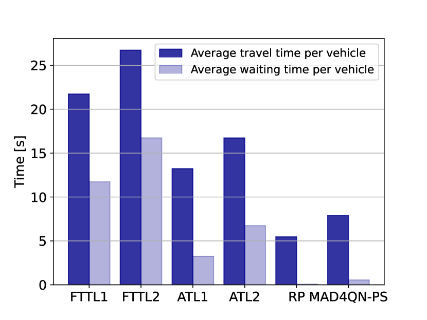
(a) Average travel and waiting time per vehicle

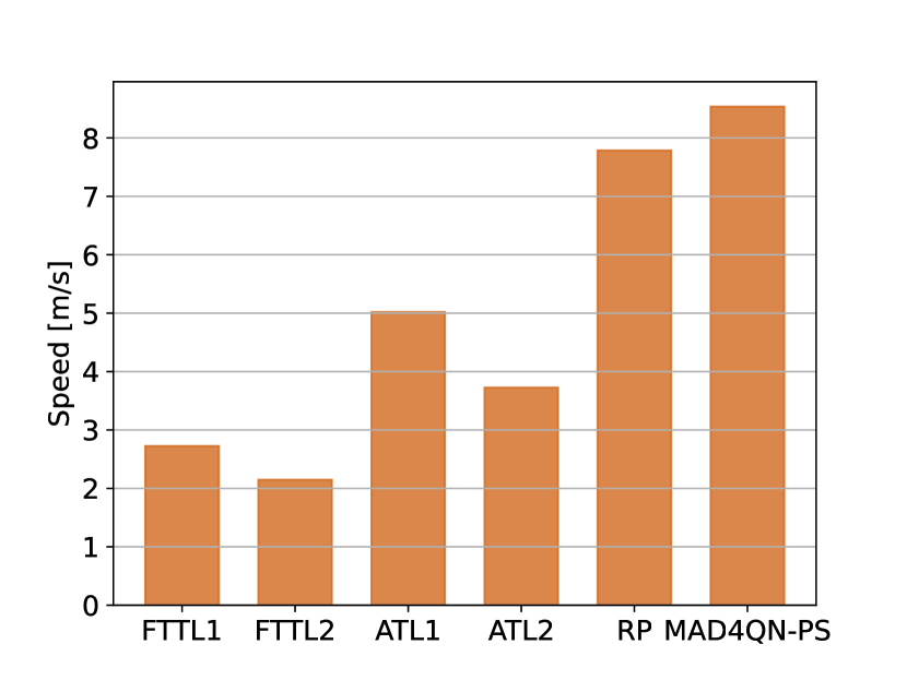
(b) Average speed per vehicle

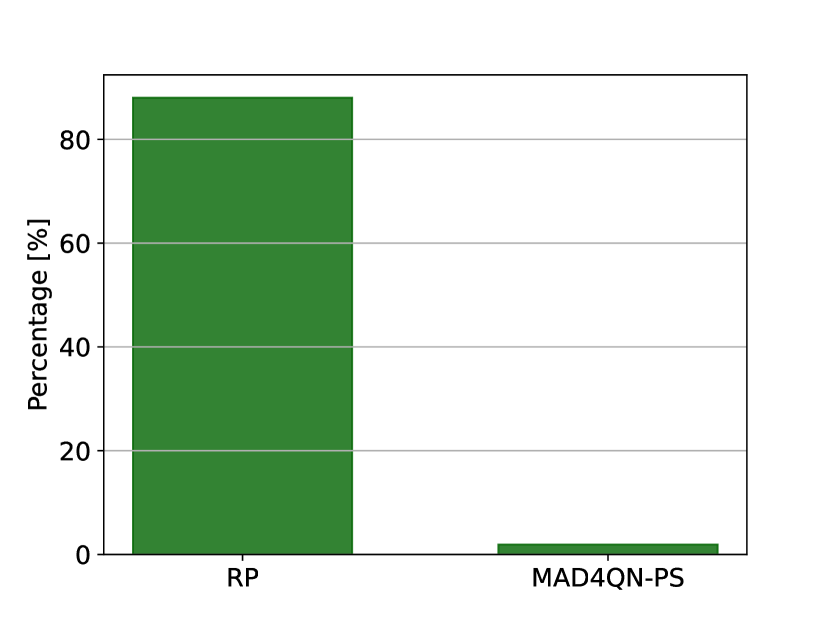
(c) Average collision rate

Figure 2: Comparison between the performance metrics of our method (MAD4QN-PS) and the baselines introduced in Section 4.1.

Lastly, we are left with the analysis of the random policy baseline, as we need to look at all the three plots to fully understand its behaviour. If we just look at Figures 2(a) and 2(b) we could argue that the random policy performance is similar to that of MAD4QN-PS. This hypothesis is however disproved by Figure 2(c), where the average collision rate for each vehicle is illustrated. The extremely high collision percentage obtained by the random policy explains why each vehicle on average spends a small amount of time with high velocity into the environment. Indeed, the simulation is terminated as soon as a vehicle crashes. MAD4QN-PS, instead, achieves an extremely low collision rate. In addition, the fact that such a collision rate is non-zero is expected and also observed in other works exploiting RL-based techniques [21, 22], given that our algorithm has to implicitly learn collision avoidance through the reward signal. In practice, the remaining failures are not problematic, because we can integrate rule-based sanity checks in the pipeline in order to be 100% collision-free. Additionally, we note that two out of the ten trained models with different seeds achieve exactly $0\%$ collision rate, meaning that if we select one of those models for deployment we are able to attain collision-free performances. This is interesting since from an applicability perspective only the best trained model would be used in practice. As a final note, we have not plotted the collision rate of the traffic lights methods for better visualization, since the latter quantity is trivially zero for all the configurations.

A short video showing the performances of MAD4QN-PS can be found at this link.

5 Conclusions and future directions

In this study, we consider a distributed approach to face the AIM paradigm. In particular, we propose a novel algorithm which exploits MARL through self-play and an original learning strategy, named prioritised scenario replay, to train three different intersection crossing agents. The derived models are stored inside CAVs, that are then able to complete their paths by choosing the model corresponding to their own turning intention while relying just on local observations. Our algorithm represents a feasible and realistic alternative to the centralised AIM concept, that is still expected to require years of technological advancement to be implementable in a real-world scenario. In addition, simulation experiments demonstrates the superior performances of our method w.r.t. classic intersection control schemes, such as static and actuated traffic lights, in terms of travel time, waiting time and average speed for each vehicle.

In future works, we aim to explore different directions for advancements. In particular, one of the main objectives is to also consider human driven vehicles inside the environment. Given the decentralised nature of the proposed method, we expect to render our algorithm more robust without dramatically change it. Conversely, significant redesign would be necessary for a centralised AIM approach. Furthermore, we envisage to test more complicated scenarios, both in terms of dimension and layout, again to improve the robustness of our algorithm. Finally, we intend to implement our algorithm in a scaled real-world scenario with miniature vehicles [43], to practically demonstrate the applicability of our method.

References

- [1] J. He, Z. Tang, X. Fu, S. Leng, F. Wu, K. Huang, J. Huang, J. Zhang, Y. Zhang, A. Radford, et al., Cooperative connected autonomous vehicles (cav): research, applications and challenges, in: 2019 IEEE 27th International Conference on Network Protocols (ICNP), 2019, pp. 1–6.
- [2] P. Kopelias, E. Demiridi, K. Vogiatzis, A. Skabardonis, V. Zafiropoulou, Connected & autonomous vehicles–environmental impacts–a review, Science of the total environment 712 (2020) 135237.
- [3] R. M. Savithramma, B. P. Ashwini, R. Sumathi, Smart mobility implementation in smart cities: A comprehensive review on state-of-art technologies, in: 2022 4th International Conference on Smart Systems and Inventive Technology (ICSSIT), 2022, pp. 10–17.
- [4] H. Yan, Y. Li, A survey of generative ai for intelligent transportation systems, arXiv preprint arXiv:2312.08248 (2023).
- [5] A. Papadoulis, M. Quddus, M. Imprialou, Evaluating the safety impact of connected and autonomous vehicles on motorways, Accident Analysis & Prevention 124 (2019) 12–22.
- [6] S. Szénási, G. Kertész, I. Felde, L. Nádai, Statistical accident analysis supporting the control of autonomous vehicles, Journal of Computational Methods in Sciences and Engineering 21 (1) (2021) 85–97.
- [7] R. N. Brewer, V. Kameswaran, Understanding the power of control in autonomous vehicles for people with vision impairment, in: Proceedings of the 20th International ACM SIGACCESS Conference on Computers and Accessibility, 2018, pp. 185–197.
- [8] B. E. Dicianno, S. Sivakanthan, S. A. Sundaram, S. Satpute, H. Kulich, E. Powers, N. Deepak, R. Russell, R. Cooper, R. A. Cooper, Systematic review: Automated vehicles and services for people with disabilities, Neuroscience Letters 761 (2021) 136103.
- [9] A. Reyes-Muñoz, J. Guerrero-Ibáñez, Vulnerable road users and connected autonomous vehicles interaction: A survey, Sensors 22 (12) (2022) 4614.
- [10] N. Hyldmar, Y. He, A. Prorok, A fleet of miniature cars for experiments in cooperative driving, in: 2019 International Conference on Robotics and Automation (ICRA), 2019, pp. 3238–3244.
- [11] A. Talebpour, H. S. Mahmassani, Influence of connected and autonomous vehicles on traffic flow stability and throughput, Transportation research part C: emerging technologies 71 (2016) 143–163.
- [12] F. Duarte, C. Ratti, The impact of autonomous vehicles on cities: A review, Journal of Urban Technology 25 (4) (2018) 3–18.
- [13] M. A. Raposo, M. Grosso, A. Mourtzouchou, J. Krause, A. Duboz, B. Ciuffo, Economic implications of a connected and automated mobility in europe, Research in transportation economics 92 (2022) 101072.
- [14] J. Conlon, J. Lin, Greenhouse gas emission impact of autonomous vehicle introduction in an urban network, Transportation Research Record 2673 (5) (2019) 142–152.
- [15] M. Taiebat, A. L. Brown, H. R. Safford, S. Qu, M. Xu, A review on energy, environmental, and sustainability implications of connected and automated vehicles, Environmental science & technology 52 (20) (2018) 11449–11465.
- [16] Ó. Silva, R. Cordera, E. González-González, S. Nogués, Environmental impacts of autonomous vehicles: A review of the scientific literature, Science of The Total Environment 830 (2022) 154615.
- [17] L. M. Schmidt, J. Brosig, A. Plinge, B. M. Eskofier, C. Mutschler, An introduction to multi-agent reinforcement learning and review of its application to autonomous mobility, in: 2022 IEEE 25th International Conference on Intelligent Transportation Systems (ITSC), 2022, pp. 1342–1349.
- [18] K. Dresner, P. Stone, Multiagent traffic management: A reservation-based intersection control mechanism, in: Autonomous Agents and Multiagent Systems, International Joint Conference on, Vol. 3, Citeseer, 2004, pp. 530–537.
- [19] P. Karthikeyan, W.-L. Chen, P.-A. Hsiung, Autonomous intersection management by using reinforcement learning, Algorithms 15 (9) (2022) 326.
- [20] J. Ayeelyan, G.-H. Lee, H.-C. Hsu, P.-A. Hsiung, Advantage actor-critic for autonomous intersection management, Vehicles 4 (4) (2022) 1391–1412.
- [21] M. Klimke, B. Völz, M. Buchholz, Cooperative behavior planning for automated driving using graph neural networks, in: 2022 IEEE Intelligent Vehicles Symposium (IV), 2022, pp. 167–174.
- [22] M. Klimke, J. Gerigk, B. Völz, M. Buchholz, An enhanced graph representation for machine learning based automatic intersection management, in: 2022 IEEE 25th International Conference on Intelligent Transportation Systems (ITSC), 2022, pp. 523–530.
- [23] D. Li, H. Pan, G. Liu, Safe and adaptive decision algorithm of automated vehicle for unsignalized intersection driving, Journal of the Brazilian Society of Mechanical Sciences and Engineering 45 (10) (2023) 537.
- [24] M. Liu, I. Kolmanovsky, H. E. Tseng, S. Huang, D. Filev, A. Girard, Potential game-based decision-making for autonomous driving, IEEE Transactions on Intelligent Transportation Systems 24 (8) (2023) 8014–8027.
- [25] G.-P. Antonio, C. Maria-Dolores, Multi-agent deep reinforcement learning to manage connected autonomous vehicles at tomorrow’s intersections, IEEE Transactions on Vehicular Technology 71 (7) (2022) 7033–7043.
- [26] Y. Gao, C. Lin, Y. Zhao, X. Wang, S. Wei, Q. Huang, 3-d surround view for advanced driver assistance systems, IEEE Transactions on Intelligent Transportation Systems 19 (1) (2017) 320–328.
- [27] D. Chakraborty, P. Stone, Multiagent learning in the presence of memory-bounded agents, Autonomous agents and multi-agent systems 28 (2014) 182–213.
- [28] T. Schaul, J. Quan, I. Antonoglou, D. Silver, Prioritized experience replay, arXiv preprint arXiv:1511.05952 (2015).
- [29] M. Zhou, J. Luo, J. Villella, Y. Yang, D. Rusu, J. Miao, W. Zhang, M. Alban, I. Fadakar, Z. Chen, et al., Smarts: An open-source scalable multi-agent rl training school for autonomous driving, in: Conference on Robot Learning, PMLR, 2021, pp. 264–285.
- [30] R. S. Sutton, A. G. Barto, Reinforcement learning: An introduction, MIT press, 2018.
- [31] R. Bellman, A markovian decision process, Journal of mathematics and mechanics (1957) 679–684.
- [32] C. J. C. H. Watkins, Learning from delayed rewards (1989).
- [33] V. Mnih, K. Kavukcuoglu, D. Silver, A. A. Rusu, J. Veness, M. G. Bellemare, A. Graves, M. Riedmiller, A. K. Fidjeland, G. Ostrovski, et al., Human-level control through deep reinforcement learning, nature 518 (7540) (2015) 529–533.
- [34] L. S. Shapley, Stochastic games, Proceedings of the national academy of sciences 39 (10) (1953) 1095–1100.
- [35] S. V. Albrecht, F. Christianos, L. Schäfer, Multi-agent reinforcement learning: Foundations and modern approaches, Massachusetts Institute of Technology: Cambridge, MA, USA (2023).
-
[36]
P. A. Lopez, M. Behrisch, L. Bieker-Walz, J. Erdmann, Y.-P. Flötteröd, R. Hilbrich, L. Lücken, J. Rummel, P. Wagner, E. Wießner, Microscopic traffic simulation using sumo, in: The 21st IEEE International Conference on Intelligent Transportation Systems, 2018.
URL https://elib.dlr.de/124092/ - [37] H. Van Hasselt, A. Guez, D. Silver, Deep reinforcement learning with double q-learning, in: Proceedings of the AAAI conference on artificial intelligence, Vol. 30, 2016.
- [38] Z. Wang, T. Schaul, M. Hessel, H. Hasselt, M. Lanctot, N. Freitas, Dueling network architectures for deep reinforcement learning, in: International conference on machine learning, PMLR, 2016, pp. 1995–2003.
-
[39]
M. Towers, J. K. Terry, A. Kwiatkowski, J. U. Balis, G. d. Cola, T. Deleu, M. Goulão, A. Kallinteris, A. KG, M. Krimmel, R. Perez-Vicente, A. Pierré, S. Schulhoff, J. J. Tai, A. T. J. Shen, O. G. Younis, Gymnasium (Mar. 2023).
doi:10.5281/zenodo.8127026.
URL https://zenodo.org/record/8127025 - [40] A. Paszke, S. Gross, S. Chintala, G. Chanan, E. Yang, Z. DeVito, Z. Lin, A. Desmaison, L. Antiga, A. Lerer, Automatic differentiation in pytorch (2017).
- [41] G. Hinton, N. Srivastava, K. Swersky, Lecture 6a overview of mini–batch gradient descent, Coursera Lecture slides https://class. coursera. org/neuralnets-2012-001/lecture,[Online (2012).
- [42] C. Wu, A. R. Kreidieh, K. Parvate, E. Vinitsky, A. M. Bayen, Flow: A modular learning framework for mixed autonomy traffic, IEEE Transactions on Robotics 38 (2) (2021) 1270–1286.
- [43] L. Paull, J. Tani, H. Ahn, J. Alonso-Mora, L. Carlone, M. Cap, Y. F. Chen, C. Choi, J. Dusek, Y. Fang, et al., Duckietown: an open, inexpensive and flexible platform for autonomy education and research, in: 2017 IEEE International Conference on Robotics and Automation (ICRA), 2017, pp. 1497–1504.