Optimal design of experiments in the context of machine-learning inter-atomic potentials: improving the efficiency and transferability of kernel based methods.

Abstract

Data-driven, machine learning (ML) models of atomistic interactions are often based on flexible and non-physical functions that can relate nuanced aspects of atomic arrangements into predictions of energies and forces. As a result, these potentials are as good as the training data (usually results of so-called ab initio simulations) and we need to make sure that we have enough information for a model to become sufficiently accurate, reliable and transferable. The main challenge stems from the fact that descriptors of chemical environments are often sparse high-dimensional objects without a well-defined continuous metric. Therefore, it is rather unlikely that any ad hoc method of choosing training examples will be indiscriminate, and it will be easy to fall into the trap of confirmation bias, where the same narrow and biased sampling is used to generate train- and test- sets. We will demonstrate that classical concepts of statistical planning of experiments and optimal design can help to mitigate such problems at a relatively low computational cost. The key feature of the method we will investigate is that they allow us to assess the informativeness of data (how much we can improve the model by adding/swapping a training example) and verify if the training is feasible with the current set before obtaining any reference energies and forces – a so-called off-line approach. In other words, we are focusing on an approach that is easy to implement and doesn’t require sophisticated frameworks that involve automated access to high-performance computational (HPC).

1 Introduction

Inter-atomic potentials are surrogate models replacing complex quantum-mechanical (QM) calculations with fast-to-evaluate functions, directly or indirectly dependent on the positions of atoms, returning forces and energies. With such potentials, we can simulate millions of atoms at timescales of nanoseconds or microseconds; something beyond the reach of QM models.

When regarded as a regression problem, the development of these potentials is challenging. Firstly, the problem cannot be easily formulated using a space with a comprehensive metric (e.g. $\mathbb{R}^{3\times N}$, $N$ being a number of atoms). A useful potential needs to be applicable to a variety of configurations requiring different numbers of atoms in a computational cell. Hence, the map, linking to energies and forces, will be defined (implicitly) on a collection of positions of various sizes. For this reason alone, formulation of potentials will be facilitated by descriptors of chemical environments – functions that represent a collection of atoms as a vector, tensor or a set (with the simplest form being a list of pairwise distances). As a result, we have two, rather than one, consecutive and non-trivial relationships. The first maps the positions of atoms to their abstract representatives and is defined by our decision to use a particular descriptor. The second is defined by a function that accepts a descriptor as an input and outputs energies and/or forces. This has been illustrated on the example of the embedded-atom model (EAM) (see e.g. A.F. Voter in [1, 2]) in fig 1.

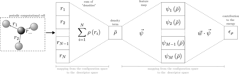
Figure 1: Illustration of the problem of double mapping using the example of the EAM model. Here we focus only on the contribution of a specific atom to the total energy and consider only the embedding representing the many-body interactions. The density $\bar{\rho}$ in principle refers to the local electronic density and consists of contributions $\rho\left(r_{i}\right)$ from neighbouring atoms, where $\rho$ is a non-linear function that can also depend on adjustable parameters, while $r_{i}$ represents the distance to a specific neighbour. We also assume that considering the first N neighbours provides almost complete information. The quantity $\bar{\rho}$ can be considered as a 1-dimensional descriptor of the local environment. The contribution to the energy will be a non-linear function of this quantity. However, in this example we assume that it can be expressed in a linear basis to illustrate the model complexity represented by the number of features M. An example of a feature can be $\bar{\rho}$ raised to the k-th power in the polynomial representation of the mapping.

For example, when we wish to train an inter-atomic potential, we need to choose a suitable descriptor and determine the right model complexity. This way, we can maximise the precision of the fit without introducing a bias. However, it is easy to make a mistake by selecting a simple descriptor that cannot differentiate between many distinct chemical environments. At the same time, we can define a very flexible regression model that can accommodate all the differences in the training data. As a result, we will encounter the problem of over-fitting despite defining a model with the right overall capacity. This is not an unusual problem in development of EAM potentials.

In response to such challenges, researchers are turning to machine-learning methods, such as, after [3], Neural Network Potentials [4], kernel based methods like the GAP – the framework for ‘atomistic’ Gaussian process regression [5] and Gradient-domain Machine Learning models [6], Moment Tensor Potentials (MTP) [7, 8], methods with a physically inspired basis like Atomic Cluster Expansion (ACE) [9], and many others [10, 11].

In this paper we focus on methods that are coupled with extensive, or rather ‘expressive’, descriptors, such as the SOAP (smooth overlap of atomic positions, [12]), designed to be applicable to many materials, distinguish between alloying elements and reflect nuanced many-body interactions. In other words, models flexible enough to be as good as the data provided. The price we will have to pay for high levels of accuracy is susceptibility to insufficient information. Once we decide to use descriptors and regression models that are sufficiently complex to be error-free and universal, we need to make sure that the training data is sufficient as well. This way interpolations and extrapolations will not fail as soon as we try to make predictions on examples moderately distinct from the training set.

It is deceptively tempting to manage this problem using brute force and integrate into the training set as many examples as possible. However, it can be inefficient, unreliable, and even with access to high-performance computing (HPC) facilities prohibitively expensive.

The choice of training examples are often motivated by physics and intuition. But what is a distinct training example from the perspective of a researcher, might not be distinguishable by the model or descriptor. What is informative may not be representative. For instance, a training set might be improved significantly by the inclusion of unrealistic configurations that provide better coverage of possible descriptor values. Likewise, polluting a data set with contradicting (e.g. when descriptor cannot distinguish between physically different examples) or irrelevant information might result in a loss of accuracy or performance respectively.

We need a systematic approach, as we have to navigate an extensive set of possible atomic configurations, through at least two maps (configuration – descriptor and descriptor – predictions of energies, etc.), and most likely without a metric. It is not a surprise that the development of a potential is such an extensive and risky task.

In practice, researchers often resort to using some form of active learning, like the classical Csányi et al. learn-on-the-fly approach [13], where model, or models, trained on partial training sets are used to query if new candidates are a good addition to the current set. As reported by Jinnouchi et al. in their overview, these strategies can result in a significant reduction in the time required for training [14]. Albeit, they still require access to vast computational resources and complex software infrastructure. Given that the training and assessment will likely involve shared HPC resources, with strict management policies, an infrastructure that might be difficult to implement. Furthermore, initial queries are made using models that can be significantly flawed unless the original database was already extensive at the beginning. Which brings us right back to the initial point.

Candidate searches can be more efficient if they can be done without labelling, i.e. obtaining values for associated quantities of interest, which usually means estimating energies and forces with ab initio QM calculations. With kernel methods, for example, we can use the pivoted low-rank approximations to mark a subset of candidates for labelling. After all, the idea behind this approximation is to select a subset of data that is most representative of the whole, i.e. giving the closest approximation to the full kernel matrix. This feature of labelling is even included in the original implementation of the GAP [5]. Likewise, as shown by Podryabinkin and Shapeev in their active learning scheme [15], or more recently by Lysogorskiy et al. [16], we can apply in the context of training of potentials criteria developed for statistical design of experiments, i.e. using the rigorous language of statistics to decide in advance what information to add or start with.

We argue that classical concepts of statistical planning, such as optimal design of experiments [17], many of which were developed when even supercomputers could not match the speed of today’s smartphones, can indeed provide a basis for efficient solutions to the problems outlined above. Optimality in this context means that for a given number of training examples (budget), we can choose those that minimise the uncertainty associated with the model parameters. Optimal designs are unique to linear basis function models and thus to kernel methods such as GAP [17]. Associated methods allow us to manage model uncertainty and verify the feasibility of learning before even the first calculation is made. As such, they allow rapid exploration and sifting through a large number of training examples. At the same time, they provide access to well-established measures of quality that are independent of labels/outputs. These measures are one of the main advantages of statistical planning, and a certain advantage over ‘vanilla’ active learning.

In our work, we will present how to optimise data for on kernel-based methods rather than weight-space models like ACE or MTP, as the associated optimality criteria and algorithms are less known and more difficult to implement. For the reasons outlined above, we also aim for solutions that provide optimal, or more realistically optimised, sets without the need for retraining and estimation of empirical errors. In this respect, our work is related to that of Karabin and Perez [18]. However, we focus on methods that aim to find optimal solutions by directly considering optimality criteria rooted in statistical theory.

2 Methodology

To emphasise the key characteristic of designs we are focusing on, we refer to them as a priori designs. As mentioned before, an optimal training set can be constructed before any ab initio calculation or experiment is made. The key is to choose an appropriate measure. For example, in linear regression with constant normally distributed ‘noise’, the variance-covariance matrix of regression coefficients is $\Sigma=\sigma^{2}\left(X^{\top}X\right)^{-1}$, where $\sigma^{2}$ is the variance of the ‘noise’, and $X$ is the design matrix – our usual assembly of inputs associated with features. It immediately transpires that by selecting appropriate inputs to $X$, we can minimise $\Sigma$ and we do not need any knowledge about the $\sigma^{2}$ (often it is a const. value) or outputs (the $y$ ’s) in our data set. More details can be found in appendix A.

There are many well-established criteria for optimality of designs that are more suitable than the direct optimisation of $\Sigma$. The most common is the D – optimality that seeks to maximise the determinant of the observed Fisher information matrix, which is given by $\sigma^{-2}X^{\top}X$ for linear models with the constant ‘noise’ (notice the similarity with the formulation of $\Sigma$). This particular criterion was used in earlier work by Podryabinkin and Shapeev to mark candidates for evaluation/labelling [15]. However, we have to keep in mind, that each family of models, be it ordinary least-squares or kernelised ridge regression (KRR, [19]), will require different strategies and criteria of optimality. Moreover, non-linear models will have only local optimal designs for a specific range of parameters [17].

In our work, we focus on the GAP model framework of Gaussian process regression (GPR). This framework can be categorised as state-of-the-art atomistic modelling that can give predictions almost as good as the training data.

To reiterate argument from the introduction, high-quality data, usually in the form of atomic configurations and associated energies and forces, are expensive to generate, even with modern hardware and efficient implementations of the density functional theory (DFT) [20]. Furthermore, we would like to use the model to make predictions on extensive computational cells that are beyond the reach of the DFT method rather than interpolate a large number of calculations. Hence, we cannot test the model by comparing it with a reference, nor can we rely on the model prediction variance as it is unreliable when it comes to highlighting errors in the definition of the descriptor. All this renders any form of active learning a less appealing choice.

To address design criteria for GPR, and as such GAP, we need to refer to the fundamentals. A Gaussian process (GP) is a collection of random variables with joint Gaussian distribution

$$f\left(\vec{x}\right)\sim\mathcal{GP}\left(m\left(\vec{x}\right),k\left(\vec{x}\right)\right),$$

specified by mean function $m$ and covariance function $k$. The model, specified by rules to evaluate $m$ and $k$, is defined by the posterior distribution conditioned on the data ([21], chapter 2). In the GPR framework, each element of the training set and each extrapolation point corresponds to a degree of freedom of a multivariate Gaussian distribution. The expectation and variance of this distribution are defined by a kernel matrix - a matrix of inner products between all data points (training and predictions). Formulation of GPR and the framework in the context of atomistic modelling can be found in [22] and [23].

The GPR can be regarded as a linear method with respect to weights (model parameters) if we choose to formulate it in the so-called weight-space view. In the function-space view, it is strongly related to KRR. Both methods share the same estimator of expectation if the penalty corresponds to the prior variance (data ‘noise’).

Relationships between these methods suggest that optimal designs are to some extent transferable. However, we need to be careful. In our experiments, when we tried to minimise the maximum prediction variance of the KRR model in an active learning framework, we created a dataset that was performing worse, when used to train a GAP model, than the source-sampling. Here, the source-sampling is a method that is used to generate a large number of candidates, that are later reduced by the algorithm to create an optimised training set.

The most straightforward design for GPR is the maximum entropy (MaxEnt) sampling introduced by Shewry and Wynn in [24]. We refer here to the entropy defined as the expectation of information content, also known as the Shannon information. In principle, it is a different quantity the entropy defined in physics. The optimality criterion authors propose (section 4) is

$$\max\log\det\mathbf{K},$$ (1)

where $\mathbf{K}$ is the covariance matrix of the multivariate Gaussian. This is the part of the covariance matrix associated with the training data in the GPR framework.

As discussed by the authors, this criterion attempts to maximise the variability in the training set. In other words, their distinctiveness and the coverage of the domain. Initially, we used this criterion in combination with a modified exchange algorithm [25], i.e. an algorithm that swaps candidates in the training set with the pool of potential replacements until the set becomes an optimal representation of the domain. However, we were concerned with its low efficiency of exploration as the algorithm required, to be computationally efficient, generating a covariance matrix for all the data, limiting the number of candidates we can consider at the same time.

For this reason, we decided to apply a conditional max-min design with an algorithm presented in [26] that performed well in comparison with our previous solutions. This design aims to maximise the minimum distance between samples. The algorithm is illustrated in figure [fig:the_alg]. A simple and efficient implementation of this algorithm can be found in the appendix B, as well as in [27] along with its applications in other contexts.

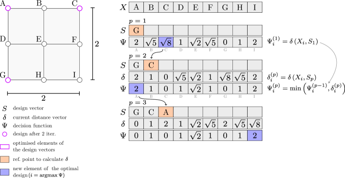
Figure 2: Illustration of the Golchi and Loeppky algorithm [26] for max-min designs, which maximises the minimum distance, using the example of nine points on a square grid. The state in each iteration is defined by the design vector $S$ and vector $\Psi$. The vector $\Psi$ can be considered as a ’decision’ function while $X$ represents the pool of candidates. Initially, $\Psi$ consists of distances between the first element and the remaining elements. In the following iterations, $\Psi$ is updated element-wise according to $\Psi_{i}^{(p)}=\min\left(\Psi_{i}^{(p-1)},\delta_{i}^{(p)}\right)$, where p is the iteration index, $\delta_{i}^{(p)}$ is the distance between $p\mathrm{-th}$ and $i\mathrm{-th}$ candidate and $\delta\left(\cdot\right)$ is the distance function. In each iteration we find the maximum value of update $\Psi$. Position of this element indicates the new optimal design point.

It proceeds in a greedy manner, i.e. candidates are ordered in terms of importance, starting with the most informative examples, in other words the most distanced. As the distance, we choose the squared kernel distance ([28])

$$D_{K}^{2}=k\left(p,p\right)+k\left(q,q\right)-2k\left(p,q\right),$$ (2)

where $K$ is the covariance function between configurations $p$ and $q$. We chose a measure based on the similarity kernel in order to create a design that is directly related to the regression method. Here, we used a complete covariance, as described in [22], consisting of radial-basis functions for pair-potentials and a polynomial kernel with the SOAP descriptor for many-body interactions. Defining the distance in such a way also i consistent with optimality criterion 1 (see figure 3).

According to our experiments with the Euclidean metric and highly biased sampling, the algorithm generates space-filling designs that embrace the whole domain. For linear least-squares regression, such designs also tend to minimise maximum prediction variance, and as such, they are consistent with the aims of G–optimality [29, 30]. Figure 3 demonstrates the test of the algorithm on a simple example of two-dimensional Cartesian space.

The distance is the same as in 2. However, in this example we selected the Gaussian kernel. As such, the solution is an optimised set with respect to the performance of the GPR regression, rather than optimal filling of the space. Although, for a Gaussian kernel with a large scale parameter these goals will coincide.

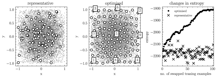
Figure 3: Application of the Golchi and Loeppky algorithm [26] for max-min designs. In this example, we are optimising the training set for Gaussian process regression. The distance measure follows the definition 2 and is based on a Gaussian kernel with unit scale parameter. The training points are selected from a pool of candidates generated using strongly biased sampling. This pool consist of $10^{4}$ samples from the normal distribution $\mathcal{N}\left(0,0.5\right)$. On the plots they are represented by small grey points with opacity. Such an example simulates conditions under which we have to select atomistic configuration for training of ML potentials. The first plot on the left illustrates a representative design, which is a random sub-sample of 100 candidates. This plot also illustrates how biased the underlying sampling is. Next, in the middle, we show the distribution in the optimised training set, also consisting of 100 examples. The index indicates the order of addition of the first 9 optimal points, revealing the algorithm’s strategy of filling empty spaces after enclosing a domain. Finally, the plot on the right shows how the entropy changes when we replace the random/representative examples with the optimised ones. Entropy for representative sets corresponds to different realisations of this design. Here, the entropy of the resulting kernel matrix $K$ is proportional to $\log\left(\det K\right)$ [24]. Note that the aim is not to provide a uniform importance sampling, but optimal training points for a given regression method. In this case, however, these objectives coincide so that we can visually assess the quality of the solution. Other models may have a different solution. See the example a) in figure 7. Finally, this results can be easily recreated using the alghorithm 2 from appendix B. We only need to replace the

3 Numerical (in silico) experiment

It is reasonable to begin the development of a training database for GAP with a collection of examples that will inform the model about elastic deformations (see e.g. [31]). This first step will serve as our case study. In other words, we wish to create a database of elastically deformed structures such that we can predict the elastic energy density of a pure Zr lattice. Our single training database will consist of 1000 examples and include hcp, fcc and bcc structures.

To create an optimised training set, allowing us to train a more accurate model, first, we generate an as extensive as possible set of candidates. The core idea behind the optimisation is to sift through contenders. Bear in mind that an empirical model is as good as the data it interpolates. Hence, we need to make sure the space is covered appropriately and that we have a sufficiently good source-sampling – one that can draw from every possibility, here defined by the structure and the strain state, with a reasonable, but not necessarily optimal, probability.

Each time, the transformation matrix, used to deform a randomly picked structure, is generated from a random uniform vector of eigenvalues (we essentially reversed the eigenvalue decomposition) and rotated using Euler angles picked indiscriminately from the group of 3D rotations.

Initially, we generated the deformation using uniform sampling of the elements of the strain tensor. However, in our experiments this sampling was severely under-performing. As such, optimised sets were always significantly better and it was difficult to judge the results against the ‘random’ sampling. In addition, we could see the benefits of the statistical planning right from the beginning as it forced us to improve the framework.

In the case study we used a converged candidate set size of 100,000 from which we selected 1000 candidates using the framework we discussed earlier, i.e. the conditional max-min design with the greedy algorithm [26].

As planned for the final atomistic model, the kernel matrix for the data-set optimisation consisted of two components. We used the Gaussian kernel to estimate pair-wise interactions, with a scaling factor of 0.8 and a length scale of 0.3, while for many body interactions, we selected the SOAP descriptor and 4th-order polynomial with a 0.3 scaling factor. The SOAP descriptor was initiated with the following string defining the parameters: soap cutoff=6.8 l_max=10 n_max=10 normalize=T atom_sigma=0.15 n_Z=1 Z={40}. The cut-off of the pair-wise distance descriptor was set to 7.0. Parameters were selected by attempting to minimise the number of overlapping (kernel distance close to zero) and orthogonal (kernel distance close to 1) examples in the trial candidate set. In other words, we selected a descriptor that can distinguish between the most similar chemical environments and, at the same time, that won’t be too sensitive to changes in atomic positions and lose the ability to quantify similarity of most distinct configurations (clipping effect).

Reference data (labels for training sets) were evaluated using the DFT method implemented in VASP [32, 33, 34, 35]. We choose the APW basis with an energy cut-off of 600 eV, automatic determination of number of k-points (with 60 subdivisions) and Methfessel-Paxton smearing method [36].

For a given training set, having obtained energies, forces and virials, we optimised kernel hyper-parameters $\theta$ (parameters of descriptors) by maximising the log-likelihood:

$$\mathcal{L}\left(\theta\right)=-\frac{1}{2}\left(y^{\top}Q^{-1}y+\ln\det(Q)+n\ln\left(2\pi\right)\right),$$

where $Q=K+\sigma I$, $Q$ is the kernel matrix of the additive model (pair-potential and the SOAP kernel) and $\sigma$ is the prior variance of the data. In the above, $y$’s are DFT energies and the optimal solution does depend on the results. Therefore, each data set will have a separate set of associated optimal parameters.

Using the optimised training set and meta-parameters we trained a GAP model using the gap_fit program from the QUIP library [5]. Contrary to the optimisation of hyper-parameters, the model fit was conducted using forces and virials as well. This way we can asses the practicality of our approach.

4 Results and conclusions

In this section, we will assess the methodology and the implementation of the algorithm. We begin by investigating how the algorithm affects the similarity of the training examples.

We compare the randomly selected (’representative’) deformed structures with those from the optimised set. The results are shown in figure 4.

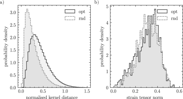
Figure 4: Comparison of pairwise distances within a random and an optimised training set. Figure a) shows normalised probability histograms of the kernel distance. Figure b) shows the distribution within a training set of the $L_{2}$norm of the deformation tensor, which we use to quantify its magnitude. The lack of a strong difference between the locations of these distributions shows that the reduction in overlap has not been achieved by simply pushing the "amount" of deformation.

It is immediately apparent that the algorithm works by removing overlapping examples and emphasising diversity, as indicated by the shift of the entire distribution, including the minimum, towards larger distances. Note that the opposite of overlap is when all examples are orthogonal and the dissimilarity, i.e. the kernel distance, is 2 in our case, as we have omitted the normalisation in equation 2.

Keep in mind that a successful optimisation is not always guaranteed. When using high-dimensional descriptors and kernel-based distances, the algorithm may favour solutions where all examples are orthogonal to each other. This would mean that the training set is useless for models that are supposed to be interpolators. We can fall into this trap by selecting extremely deformed examples. Therefore, we had to restrict the search space accordingly. In our case, we did this by limiting the maximum eigenvalues of the deformation matrix. This highlights the key chellenge of the presented methodology, which is the choice of the distance or dissimilarity measure.

While we demonstrated that the methodology improves the quality of a training set, we need to show that this change is significant in a realistic scenario. To do this, we generated two optimised training sets, OPT1 and OPT2, consisting of 1000 examples selected from two independent pools of candidates (100,000 per pool). Additionally, from each we selected randomly and indiscriminately a subset of 1000 candidates, creating two representative training sets: RND1 and RND2. Here, OPT stands for ‘optimised’ and RND for ‘random’ or representative of the source-sampling.

The idea is to gauge how much improvement the optimisation introduced by comparing models trained on each set. The procedure is closely related to the concept of cross-validation. In the assessment, we utilised all DFT energies and GAP predictions made on all configurations. Having four training sets and, as such, four models, we can make 16 comparisons in total. For example, we take the GAP model trained on the OPT1, evaluate energies on configurations from OPT1, OPT2, RND1, RND2 and compare GAP predictions with DFT references. When we test the model predictions on its own training set, essentially, we evaluate the goodness of fit. Otherwise, we are enquiring about the off-sample performance. Results are presented in figure 6 and 6.

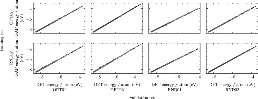
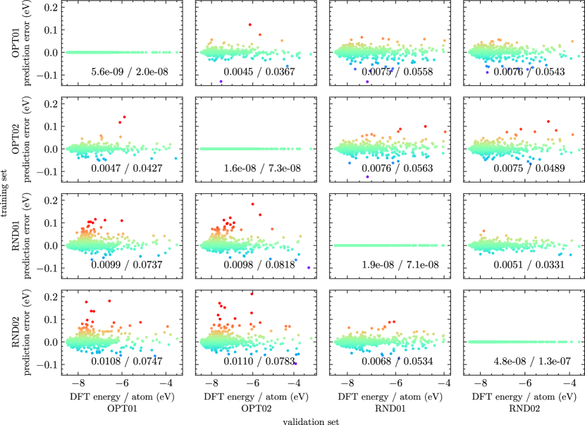
Figure 5: Examples of performance when predicting energy per atom on training and validation sets. Brightness indicates prediction error from fig. 6.

Figure 6: Results of cross-validation. Here (GAP) models are defined by their corresponding training sets and organised in rows. Each column corresponds to validation set on which model was tested. Plots on the diagonal illustrate fitting performance. Colour indicates the position on the y-axis. Summary statistics are: standard deviation (first number in the label) of the absolute error (DFT results versus GAP prediction), and 0.99 quantile (second number in the label).

It immediately transpires that the optimised training sets delivered a more consistent and overall better performance than their representative (random) counterparts. Here, we measure the performance as the worst off-sample performance given by the highest, among all test sets, 0.99 quantile of the absolute error. We demonstrated that we can achieve better transferability in exchange for some level of precision in a more narrow context. In other words, optimised sets are likely to have a better coverage of the whole domain in exchange for fewer samples around the mode of the source-sampling, i.e. the distribution to generate the initial pools of candidates. It is exactly what we expect from the optimal design. The argument is reinforced by the fact that models trained on RND1 and RND2 sets did well when tested against each others corresponding training sets. At the same time, when evaluated on OPT sets, their performance was worse than the worst performance of OPT models.

There are two main considerations that we have to keep in mind when interpreting the results. First, the underlying generation of training examples has already been improved as a result of initial analysis in the context of statistical planning. However, it is not always easy to improve the source-sampling as it was in the case of elastic deformations of perfect lattices. Secondly, in the optimisation we used a kernel matrix associated with energies. Yet the final training sets also consisted of forces and virials as a part of associated labels/outputs. Therefore, we have shown that even a simplified methodology can provide quantifiable benefits in realistic scenarios.

In summary, we demonstrated that the optimal design and statistical planning is an effective tool that can improve the reliability and generalisability of data-driven models. The two main advantages over the active learning are providing measures of quality that allow comparison of training sets and the ability to improve them without the necessity of evaluating labels, i.e. in this context, energies, forces and virials.

At the same time, we demonstrated that empirical methods of performance evaluation, such as the well-known test-train-split framework, should be applied carefully. It is relatively easy to overestimate the predictive power of a model and fall into the trap of confirmation bias. As we saw when comparing representative sets.

For example, when the method of creating training examples probes only a narrow part of a domain, we obtain "dense" sampling that can give us deceptively good interpolations in this region. While it is not a problem in Euclidean spaces, with the high-dimensional descriptors, it might be extremely difficult, or even impossible, to define a metric that will allow us to sample the domain "uniformly". In other words, we always have to keep in mind that we are always in danger of replicating biases introduced by the source-sampling.

The statistical planning of experiments may help us to overcome these challenges. However, only when certain conditions are satisfied. First, we can select from a large enough pool of candidates. Secondly, we have a method to adequately sample the whole domain.

The application of optimal design in the context of ML potentials is still relatively unique. Hence, there are many areas for potential development. First, we need ways to define sufficiently good underlying sampling, especially for many body representations. We suggest that developments related to exploring configuration space are aligning with this goal and can be used to ensure appropriate coverage of the descriptor space. Secondly, another essential part of the methodology is the efficient optimisation algorithm. The conditional max-min design or exchange algorithms can be adequate only when descriptors, or the kernel matrix, are precalculated. Therefore, for large sets of candidates, memory requirements can be limiting, and there is a need for efficient lazy algorithms.

5 Acknowledgements

We would like to kindly acknowledge The Engineering and Physical Sciences Research Council (EPSRC) for funding the MIDAS project (Mechanistic understanding of Irradiation Damage in fuel Assemblies – ref. EP/S01702X/1). C P Race was funded by a University Research Fellowship of the Royal Society. Calculations were performed on a computational cluster, maintained by the Computational Shared Facility, The University of Manchester.

6 Author contributions

Bartosz Barzdajn: Writing - Original draft, Conceptualization, Methodology, Software, Validation, Formal analysis, Investigation, Data curation, Visualization. Christopher Race: Writing - Review \& Editing, Conceptualization, Methodology, Validation, Formal analysis, Supervision, Project administration, Funding acquisition.

Appendix A Introducing the concept of the optimal design

We will illustrate the concept of optimal design using the simplest regression model

$$y=Xw+e,$$

where $y$ is a vector of observed values (labels), $X$ is the design matrix with $i$-th row representing observation $x_{i}$ and defined by a vector-valued feature map $\phi\left(x_{i}\right)$ (e.g. in polynomial regression $\phi_{k}\left(x_{i}\right)=x_{i}^{k}$ with $k$ ranging from $0$ to the order of a polynomial), $w$ is a vector of model parameters and $e$ is a disturbance term (assume symmetric uni-modal distribution of $e$ and $\mathrm{cov}\left(e\right)=\sigma^{2}I$). Obviously, we want to find the model parameters with a minimum number of training examples and a minimum uncertainty.

Consider the example of D-optimality which aims to maximise the determinant of the Fisher information matrix (FIM). For least-square estimators FIM is simply given as $\mathscr{I}=\sigma^{-2}X^{\top}X$. It is related to the covariance of $w$ which is given by $\Sigma=\sigma^{2}\left(X^{\top}X\right)^{-1}$. Hence, by maximising the information $\mathscr{I}$ we minimise the uncertainty $\Sigma$. We see that the objective can be achieved without referring to $y$’s at all and that we can quantify the effect of selecting different training examples without $\sigma$, i.e. the noise/uncertainty associated with the data. Hence, the optimal design will be a function solely of $X$ . An example of applying an optimal design to a simple polynomial model can be found in figure 7.

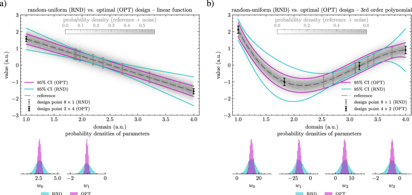
Figure 7: Comparison of optimal design (D-optimality) for polynomial regression with randomly selected point from a domain. Note that all points were selected before making estimates. Confidence interval (CI) and density of˙parameters are estimated using Monte Carlo (MC) method with $5\times 10^{4}$ samples. Error bars represent design points, i.e. points where ‘measurements’ were made in each MC iteration. Functions and their parameters are defined as follows: $f(x)=w_{0}x^{0}+w_{1}x^{1}+\ldots w_{N}x^{N}.$ Space-filling designs will yield similar results to the optimal design. Note that significant difference in the performance is emphasised by the unfavourable sample.

In this example, we intentionally used random uniform sampling rather than the equal division of the domain. While the latter seems like a natural choice, when the feature space is high-dimensional, some form of random sampling is considered to be an adequate solution. Therefore, the results can be considered as a representative illustration of the benefits that optimal design can provide. Furthermore, by selecting low-order polynomials, we can show that optimal designs can differ from the usual intuition. While after some careful consideration, we could conclude that the best design for linear models is to concentrate our whole budget on the edges of the domain, the $4\times 2$ (four points sampled twice) can be considered as more difficult to foresee without formal calculations. Particularly, it can be difficult in high-dimensional and non-Euclidiean spaces.

Note that there are other popular criteria such as the A-optimality – minimise $\mathrm{tr}\Sigma$, E-optimality – maximise minimal eigenvalue of $\mathscr{I}$ or G-optimality which seeks to minimise the maximum prediction variance [17]. These are just few examples and an appropriate selection will depend on the family of models and expectations with respect to the performance of estimators.

Appendix B Example of the implementation in Python

In this section we present a simple implementation of the conditional max-min design (figure 2) using the example of two-dimensional Euclidean space. This will be a case of space filing design which is well performing design overall and it is close to optimal for polynomials of high degree or kernel based methods with Gaussian kernel.

We start by generating the pool of candidates. Here it will be a dense uniform grid of points covering the entire domain $\left[-1,1\right]\times\left[-1,1\right]$. The Python code using the NumPy library, imported under the ’np’ label, can be found in the listing 1.

⬇

x1, x2 = np.mgrid[-1:1.05:.05, -1:1.05:0.05]

x1, x2 = x1.flatten(), x2.flatten()

X = np.vstack((x1, x2)).T

rng = np.random.default_rng()

X = rng.permutation(X, axis=0)

Algorithm 1 Generation of uniform grid of points.

In the context of ML potentials, in realistic scenarios we do not have well-defined metric, and even random uniform sampling is impossible or impractical, let alone the importance sampling. However, such an idealised test case allows for an easier assessment of the algorithm and its implementation.

The main optimisation loop, presented in listing 2, has a very simple implementation that takes advantage of vectorised element-wise operations.

⬇

def delta(x, y, p=2):

return np.linalg.norm(x - y, axis=1, ord=p)

i = np.argmax(np.linalg.norm(X, axis=1))

X[[0, i]] = X[[i, 0]]

S = [0] Psi = delta(X, X[S[0]])

for k in range(40):

Psi = np.minimum(Psi, delta(X, X[S[-1]]))

S.append(np.argmax(Psi))

Algorithm 2 Selection of optimal training points.

The distance between elements is defined by the Euclidean distance ($L_{2}$ norm). The results of the optimisation are presented in figure 8.

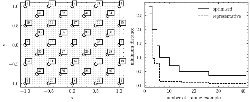
Figure 8: Illustration of the max-min design. On the left, optimal points selected form a candidates distributed on a regular grid. Ordering is ‘random’. Labels indicate in which order points were added to the design. On the right, minimum distance of the max-min design compared to random, indiscriminate selection of candidates.

Here, we will omit implementation of the code used to generate figures and calculate the minimum distance.

As in the example from figure 3, given the budget, the algorithm tries to cover the whole space evenly and embrace the whole domain. This is an important feature, as it allow us to adjust the budget simply by selecting first $n$ candidates.

References

- [1] J H Westbrook and R L Fleischer, editors. Intermetallic Compounds. John Wiley & Sons.
- [2] A.F. Voter. The Embedded-Atom Method. URL: https://public.lanl.gov/afv/VoterEAMchapter.pdf.
- [3] Emir Kocer, Tsz Wai Ko, and Jörg Behler. Neural Network Potentials: A Concise Overview of Methods. 73(1):163–186. URL: https://www.annualreviews.org/doi/10.1146/annurev-physchem-082720-034254, doi:10.1146/annurev-physchem-082720-034254.
- [4] Sönke Lorenz, Axel Groß, and Matthias Scheffler. Representing high-dimensional potential-energy surfaces for reactions at surfaces by neural networks. 395(4-6):210–215. URL: https://linkinghub.elsevier.com/retrieve/pii/S000926140401125X, doi:10.1016/j.cplett.2004.07.076.
- [5] Albert P. Bartók, Mike C. Payne, Risi Kondor, and Gábor Csányi. Gaussian Approximation Potentials: The Accuracy of Quantum Mechanics, without the Electrons. 104(13):136403. URL: https://link.aps.org/doi/10.1103/PhysRevLett.104.136403, doi:10.1103/PhysRevLett.104.136403.
- [6] Stefan Chmiela, Huziel E. Sauceda, Klaus-Robert Müller, and Alexandre Tkatchenko. Towards exact molecular dynamics simulations with machine-learned force fields. 9(1):3887. URL: https://www.nature.com/articles/s41467-018-06169-2, doi:10.1038/s41467-018-06169-2.
- [7] Alexander V. Shapeev. Moment tensor potentials: A class of systematically improvable interatomic potentials. 14(3):1153–1173. arXiv:https://doi.org/10.1137/15M1054183, doi:10.1137/15M1054183.
- [8] Alexander V. Shapeev. Moment Tensor Potentials: A class of systematically improvable interatomic potentials. 14(3):1153–1173. URL: http://arxiv.org/abs/1512.06054, arXiv:1512.06054, doi:10.1137/15M1054183.
- [9] Ralf Drautz. Atomic cluster expansion for accurate and transferable interatomic potentials. 99(1):014104. URL: https://link.aps.org/doi/10.1103/PhysRevB.99.014104, doi:10.1103/PhysRevB.99.014104.
- [10] Y. Mishin. Machine-learning interatomic potentials for materials science. 214:116980. URL: https://linkinghub.elsevier.com/retrieve/pii/S1359645421003608, doi:10.1016/j.actamat.2021.116980.
- [11] Pascal Friederich, Florian Häse, Jonny Proppe, and Alán Aspuru-Guzik. Machine-learned potentials for next-generation matter simulations. 20(6):750–761. URL: https://www.nature.com/articles/s41563-020-0777-6, doi:10.1038/s41563-020-0777-6.
- [12] Albert P. Bartók, Risi Kondor, and Gábor Csányi. On representing chemical environments. 87(18):184115. URL: https://link.aps.org/doi/10.1103/PhysRevB.87.184115, doi:10.1103/PhysRevB.87.184115.
- [13] Gabor Csányi, T. Albaret, M. C. Payne, and A. De Vita. “Learn on the Fly”: A Hybrid Classical and Quantum-Mechanical Molecular Dynamics Simulation. 93(17):175503. URL: https://link.aps.org/doi/10.1103/PhysRevLett.93.175503, doi:10.1103/PhysRevLett.93.175503.
- [14] Ryosuke Jinnouchi, Kazutoshi Miwa, Ferenc Karsai, Georg Kresse, and Ryoji Asahi. On-the-Fly Active Learning of Interatomic Potentials for Large-Scale Atomistic Simulations. 11(17):6946–6955. URL: https://pubs.acs.org/doi/10.1021/acs.jpclett.0c01061, doi:10.1021/acs.jpclett.0c01061.
- [15] Evgeny V. Podryabinkin and Alexander V. Shapeev. Active learning of linearly parametrized interatomic potentials. 140:171–180. URL: https://linkinghub.elsevier.com/retrieve/pii/S0927025617304536, doi:10.1016/j.commatsci.2017.08.031.
- [16] Yury Lysogorskiy, Anton Bochkarev, Matous Mrovec, and Ralf Drautz. Active learning strategies for atomic cluster expansion models. 7(4):043801. URL: https://link.aps.org/doi/10.1103/PhysRevMaterials.7.043801, doi:10.1103/PhysRevMaterials.7.043801.
- [17] Dieter Rasch and Günter Herrendörfer. Statystyczne Planowanie Doświadczeń. Wydawnictwo Naukowe, PWN Sp. z o.o.
- [18] Mariia Karabin and Danny Perez. An entropy-maximization approach to automated training set generation for interatomic potentials. 153(9):094110. URL: https://pubs.aip.org/jcp/article/153/9/094110/199441/An-entropy-maximization-approach-to-automated, doi:10.1063/5.0013059.
- [19] Kevin P. Murphy. Machine Learning: A Probabilistic Perspective. Adaptive Computation and Machine Learning Series. MIT Press.
- [20] W. Kohn and L. J. Sham. Self-Consistent Equations Including Exchange and Correlation Effects. 140:A1133–A1138. URL: https://link.aps.org/doi/10.1103/PhysRev.140.A1133, doi:10.1103/PhysRev.140.A1133.
- [21] Carl Edward Rasmussen and Christopher K. I. Williams. Gaussian Processes for Machine Learning. Adaptive Computation and Machine Learning. MIT Press.
- [22] Albert P. Bartók and Gábor Csányi. Gaussian approximation potentials: A brief tutorial introduction. 115(16):1051–1057. URL: https://onlinelibrary.wiley.com/doi/10.1002/qua.24927, doi:10.1002/qua.24927.
- [23] Volker L. Deringer, Albert P. Bartók, Noam Bernstein, David M. Wilkins, Michele Ceriotti, and Gábor Csányi. Gaussian Process Regression for Materials and Molecules. 121(16):10073–10141. URL: https://pubs.acs.org/doi/10.1021/acs.chemrev.1c00022, doi:10.1021/acs.chemrev.1c00022.
- [24] M. C. Shewry and H. P. Wynn. Maximum entropy sampling. 14(2):165–170. URL: https://www.tandfonline.com/doi/full/10.1080/02664768700000020, doi:10.1080/02664768700000020.
- [25] Alan J. Miller and Nam-Ky Nguyen. Algorithm AS 295: A Fedorov Exchange Algorithm for D-Optimal Design. 43(4):669. URL: https://www.jstor.org/stable/2986264?origin=crossref, arXiv:2986264, doi:10.2307/2986264.
- [26] Shirin Golchi and Jason L. Loeppky. Monte Carlo based Designs for Constrained Domains. URL: http://arxiv.org/abs/1512.07328, arXiv:1512.07328.
- [27] Bartosz Barzdajn. Implementing conditional max-min designs in Python. May 2024. doi:10.5281/zenodo.11191242.
- [28] Jeff M. Phillips and Suresh Venkatasubramanian. A Gentle Introduction to the Kernel Distance. URL: http://arxiv.org/abs/1103.1625, arXiv:1103.1625.
- [29] M.E. Johnson, L.M. Moore, and D. Ylvisaker. Minimax and maximin distance designs. 26(2):131–148. URL: https://linkinghub.elsevier.com/retrieve/pii/037837589090122B, doi:10.1016/0378-3758(90)90122-B.
- [30] Werner G. Müllera, Luc Pronzato, and Helmut Waldl. Beyond space-filling: An illustrative case. 7:14–19. URL: https://linkinghub.elsevier.com/retrieve/pii/S1878029611001319, doi:10.1016/j.proenv.2011.07.004.
- [31] Wojciech J. Szlachta, Albert P. Bartók, and Gábor Csányi. Accuracy and transferability of Gaussian approximation potential models for tungsten. 90(10):104108. URL: https://link.aps.org/doi/10.1103/PhysRevB.90.104108, doi:10.1103/PhysRevB.90.104108.
- [32] G. Kresse and J. Furthmüller. Efficiency of ab-initio total energy calculations for metals and semiconductors using a plane-wave basis set. 6(1):15–50. URL: https://linkinghub.elsevier.com/retrieve/pii/0927025696000080, doi:10.1016/0927-0256(96)00008-0.
- [33] G. Kresse and J. Furthmüller. Efficient iterative schemes for ab initio total-energy calculations using a plane-wave basis set. 54(16):11169–11186. URL: https://link.aps.org/doi/10.1103/PhysRevB.54.11169, doi:10.1103/PhysRevB.54.11169.
- [34] G. Kresse and J. Hafner. Ab Initio molecular dynamics for liquid metals. 47(1):558–561. URL: https://link.aps.org/doi/10.1103/PhysRevB.47.558, doi:10.1103/PhysRevB.47.558.
- [35] G. Kresse and D. Joubert. From ultrasoft pseudopotentials to the projector augmented-wave method. 59(3):1758–1775. URL: https://link.aps.org/doi/10.1103/PhysRevB.59.1758, doi:10.1103/PhysRevB.59.1758.
- [36] M. Methfessel and A. T. Paxton. High-precision sampling for Brillouin-zone integration in metals. 40(6):3616–3621. URL: https://link.aps.org/doi/10.1103/PhysRevB.40.3616, doi:10.1103/PhysRevB.40.3616.