From linear programming to colliding particles

Abstract.

Although simplices are trivial from a linear optimization standpoint, the simplex algorithm can exhibit quite complex behavior. In this paper we study the behavior of max-slope pivot rules on (products of) simplices and describe the associated pivot rule polytopes. For simplices, the pivot rule polytopes are combinatorially isomorphic to associahedra. To prove this correspondence, we interpret max-slope pivot rules in terms of the combinatorics of colliding particles on a line. For prisms over simplices, we recover Stasheff’s multiplihedra. For products of two simplices we get new realizations of constrainahedra, that capture the combinatorics of certain particle systems in the plane.

1. Introduction

A linear program (LP) is an optimization problem of the form

$$\begin{array}[]{lr@{\,+\,}c@{\,+\,}r@{\,}l}\text{maximize}&c_{1}x_{1}&\cdots&c_{n}x_{n}\\ \text{subject to}&a_{i1}x_{1}&\cdots&a_{in}x_{n}&\ \leq\ b_{i}\quad\text{ for }i=1,\dots,N\,.\end{array}$$

Geometrically, the set $P\subset\mathbb{R}^{n}$ of feasible solutions is a polyhedron and a generic objective function $c=(c_{1},\dots,c_{n})$ induces an orientation on the geometric graph $G(P)$. The orientation is acyclic with a unique sink at the optimal vertex $v_{\mathrm{opt}}$. The simplex algorithm starts at a given vertex $v$ of $P$ and proceeds along directed edges to $v_{\mathrm{opt}}$. The choice which edges to pursue is governed by a pivot rule.

A polytope $P\subset\mathbb{R}^{n}$ is a simplex if its vertices are affinely independent. Simplices are trivial from an optimization viewpoint as any two vertices of $P$ are adjacent. However, sophisticated algorithms such as the simplex algorithm can exhibit complex and interesting behavior on trivial instances. In this paper, we describe a beautiful and unexpected connection between the behavior of certain pivot rules on (products of) simplices and the combinatorics of colliding particles.

A pivot rule is memory-less if its behavior on a linear program $(P,c)$ is captured by an arborescence (or rooted tree) on $G(P)$. In [2] we studied families of memory-less pivot rules that are parametrized by weight vectors $w$. We showed that for any linear program $(P,c)$ there is a polytope $\Pi(P,c)$, the pivot rule polytope, whose vertices correspond to the arborescences of $(P,c)$ induced by the family of pivot rules. The facial structure of $\Pi(P,c)$ reflects the relation between the different rules on $(P,c)$. For the max-slope pivot rule, a generalization of the shadow vertex algorithm of Gass and Saaty [9] that we introduced in [2], we were surprised to observe that the numbers of max-slope arborescences for simplices are given by the Catalan numbers. Much of the combinatorics surrounding the Catalan numbers is famously embodied by the associahedron $\mathrm{Asso}_{n-2}$, a certain partially ordered set that is ubiquitous in geometric and algebraic combinatorics. Lee [10] showed that $\mathrm{Asso}_{n-2}$ is isomorphic to the face poset of a simple $(n-2)$-dimensional polytope. Since then many different ways of realizing $\mathrm{Asso}_{n-2}$ as a polytope have been discovered in various contexts; see, for example, [6]. The present paper adds a new construction to the list.

Theorem 4.3.

Let $P$ be an $(n-1)$-dimensional simplex and $c$ a generic objective function. Then the max-slope pivot rule polytope $\Pi(P,c)$ is combinatorially isomorphic to the $(n-2)$-dimensional associahedron $\mathrm{Asso}_{n-2}$.

Associahedra describe the combinatorics of colliding particles. Consider $n$ distinct and ordered particles on the real line. Particles move, collide, and merge until there is a single particle left. The various collisions can be time-independently recorded by a bracketing. For example $(12)(345)$ states that at some point particles $1$ and $2$ collide and, earlier or later, $3,4$, and $5$ collide simultaneously. Eventually, the two remaining particles collide. The associahedron $\mathrm{Asso}_{n-2}$ is the set of bracketings of $123\dots n$ partially ordered by refinement. In order to prove 4.3, we describe a geometric correspondence between max-slope arborescences and bracketings. For that, the objective function $c$ gives rise to velocities for the $n$ particles and the weights $w$ give each particle a location at time $t=0$. For $t>0$, the particles start to move from their locations at constant velocity. If two particles collide, the slower particle is absorbed by the faster one, which continues at its original velocity. For $t\gg 0$, only particle $n$ is left. We record the particle $\mathcal{A}(i)$ that absorbs the particle $i$. Towards a proof of 4.3, we show that these maps $\mathcal{A}$, called collision patterns, are in bijection with bracketings and are precisely the max-slope arborescences of an $(n-1)$-simplex with objective function $c$.

Bottman and Poliakova [5] studied a more general setup for particle collisions. For $m,n\geq 1$, they consider $m\cdot n$ particles sitting at the intersections of $m$ horizontal and $n$ vertical lines in the plane. The particles are allowed to move horizontally or vertically but they must retain their colinearities. The collisions can be recorded by rectangular brackets or, equivalently, by a partially ordered set on the (spaces between) the horizontal and vertical lines. The resulting poset of rectangular bracketings is called the constrainahedron $C(m,n)$. For $m=1$, this is the associahedron. For $m=2$, $C(2,n)$ is isomorphic to the multiplihedron, a poset first described by Stasheff [17] and realized as a polytope by Forcey [8]. It is shown in [5], that $C(m,n)$ is the face poset of a generalized permutahedron [13]. Chapoton and Pilaud [7] introduced a remarkable operation on products of generalized permutahedra, called shuffle products, and gave a different realization of $C(m,n)$ as the shuffle product of Loday associahedra. We give new realizations of constrainahedra that, in particular, are not generalized permutahedra.

Theorem 5.8.

Let $P_{m-1,n-1}$ be the product of an $(m-1)$-simplex and an $(n-1)$-simplex and let $c$ be a generic objective function. Then the max-slope pivot rule polytope $\Pi(P_{m-1,n-1},c)$ is combinatorially isomorphic the $(m,n)$-constrainahedron $C(m,n)$.

The combinatorial construction of constrainahedra was motivated by questions in homotopical algebra [12] as well as Gromov compactifications of configuration spaces. More precisely, Bottman [4] constructed $2$-associahedra as posets capturing the behavior of ordered particles on parallel lines in the plane without colinearities. It is conjectured that $2$-associahedra are face posets of convex polytopes and we hope that our results provide a new point of view on this conjecture.

Our techniques generalize to higher products of simplices. We focus on the case in which all but one simplex is $1$-dimensional.

Theorem 6.2.

Let $(\mathbb{A},\cdot)$ be a non-associative monoid and let $f_{1},\dots,f_{k}:\mathbb{A}\to\mathbb{A}$ be morphisms. The vertices of the max-slope pivot polytope of an $(n-1)$-simplex times a $k$-cube are in bijection with the possible ways of evaluating

$$(f_{\sigma(1)}\circ f_{\sigma(2)}\circ\cdots\circ f_{\sigma(k)})(a_{1}\cdot a_{2}\cdots a_{n})\,,$$

where $a_{1},\dots,a_{n}\in\mathbb{A}$ and $\sigma\in\mathfrak{S}_{k}$ is a permutation.

These are the vertices of the $(m,n)$-multiplihedra of Chapoton and Pilaud [7]; see also [11]. In light of these results, we conjectured together with Vincent Pilaud that max-slope pivot rule polytopes of higher products of simplices are isomorphic to shuffle products of associahedra. This was proven by Germain Poullot in his thesis [14] and will appear in a forthcoming paper. We close with some results and conjectures on the enumerative combinatorics on the vertex numbers of these $(m,n)$-multiplihedra.

We collect the necessary motivation and background on max-slope pivot rules and pivot rule polytopes in Section 2. In Section 3, we develop the combinatorics of max-slope arborescences on simplices. In Section 4 we describe the correspondence to colliding particles and prove 4.3. In Section 5, we discuss products of two simplices and prove 5.8. In Section 6 we discuss higher products of simplices and focus on the simplex-times-cube case.

Acknowledgements

We would like to thank Aenne Benjes, Jesús De Loera, Vincent Pilaud, Dasha Poliakova, Alex Postnikov, Germain Poullot, and Hugh Thomas for insightful conversations. The last author would like to thank the organizers of the workshop Combinatorics and Geometry of Convex Polyhedra, held at the Simons Center for Geometry and Physics, where he first learned about constrainahedra. The first author was supported by the NSF GRFP and NSF DMS-1818969.

2. Max-slope pivot rule polytopes

We recall the necessary background on max-slope pivot rules and the associated pivot rule polytopes. We refer the reader to [2] for details and proofs.

Let $P\subset\mathbb{R}^{n}$ be a convex polytope with vertex set $V(P)=\{v_{1},\dots,v_{n}\}$. We write $E(P)$ for the edges of $P$. We call $c\in\mathbb{R}^{n}$ edge-generic with respect to $P$ if $\langle{c,u}\rangle\neq\langle{c,v}\rangle$ for all edges $uv\in E$. The vector $c$ defines an objective function $x\mapsto\langle{c,x}\rangle$ and $(P,c)$ is a linear program (LP).

We denote the unique maximizer of $c$ over $P$ by $v_{\mathrm{opt}}$. A $c$-arborescence is a map $\mathcal{A}:V(P)\setminus v_{\mathrm{opt}}\to V(P)$ such that $\mathcal{A}(v)$ is a $c$-improving neighbor of $v\neq v_{\mathrm{opt}}$. If $c$ is clear from the context, we simply call $\mathcal{A}$ an arborescence. Arborescences encode the behavior of memory-less pivot rules on the linear program $(P,c)$: From a starting vertex $v\in V(P)$, the simplex algorithm constructs a monotonically increasing path $v=v_{0}v_{1}\dots v_{m}=v_{\mathrm{opt}}$ in the graph of $P$ that satisfies $v_{i}=\mathcal{A}(v_{i-1})$ for all $i=1,\dots,m$.

The max-slope pivot rule introduced in [2] generalizes the well-known shadow-vertex simplex algorithm. For $w\in\mathbb{R}^{d}$ generic and linearly independent of $c$, we define the max-slope arborescence $\mathcal{A}^{w}$ of $(P,c)$ by

$$\mathcal{A}^{w}(v)\ :=\ \operatorname{argmax}\left\{\frac{\langle{w,u-v}\rangle}{\langle{c,u-v}\rangle}:uv\in E(P),\langle{c,u}\rangle>\langle{c,v}\rangle\right\}\,.$$ (1)

A geometric interpretation for a max-slope arborescence can be given as follows. Define the linear projection $\pi:\mathbb{R}^{n}\to\mathbb{R}^{2}$ by $\pi(x)=(\langle{c,x}\rangle,\langle{w,x}\rangle)$. The projection of an edge $uv\in E$ to the plane has a well-defined slope with respect to the $x$-axis and $\mathcal{A}^{w}(v)$ selects the edge with maximal slope.

For a $c$-arborescence $\mathcal{A}$ we define

$$\psi(\mathcal{A})\ :=\ \sum_{v\neq v_{\mathrm{opt}}}\frac{\mathcal{A}(v)-v}{\langle{c,\mathcal{A}(v)-v}\rangle}\,.$$ (2)

and the max-slope pivot rule polytope of $(P,c)$

$$\Pi(P,c)\ :=\ \operatorname{conv}\big{\{}\psi(\mathcal{A}):\mathcal{A}\text{ $c$-arborescence of }(P,c)\big{\}}\,.$$

This is a convex polytope, that geometrically encodes the various max-slope arborescences of $(P,c)$. The support function $h_{Q}:\mathbb{R}^{n}\to\mathbb{R}$ of a polytope $Q\subset\mathbb{R}^{n}$ is defined by $h_{Q}(w):=\max\{\langle{w,x}\rangle:x\in Q\}$. For $w\in\mathbb{R}^{n}$ we write $Q^{w}$ for the face $Q\cap\{x:\langle{w,x}\rangle=h_{Q}(w)\}$.

Theorem 2.1 ([2, Theorem 1.4]).

Let $P$ be a polytope and $c$ an edge-generic objective function. Then for every generic $w$

$$\Pi(P,c)^{w}\ =\ \{\psi(\mathcal{A}^{w})\}\,.$$

In particular, the vertices of $\Pi(P,c)$ are in bijection with max-slope arborescences of $(P,c)$.

The affine hull $\operatorname{aff}(P)$ of $P$ is the inclusion-minimal affine subspace containing $P$.

Proposition 2.2.

Let $P\subset\mathbb{R}^{n}$ be a polytope and $c\in\mathbb{R}^{n}$ an edge-generic objective function. Then

$$\operatorname{aff}(\Pi(P,c))\ =\ (-q+\operatorname{aff}(P))\cap\{x:\langle{c,x}\rangle=|V(P)|-1\}\,,$$

for any $q\in P$. In particular, $\dim\Pi(P,c)=\dim P-1$.

Proof.

Let $L$ denote the right-hand side of the given equation. It follows from (2) that $\psi(\mathcal{A})\in L$ for every arborescence $\mathcal{A}$ and hence $\operatorname{aff}(\Pi(P,c))\subseteq L$. Since $c$ is not constant on $P$, it follows that $L$ is of dimension $\dim P-1$. Theorem 1.4 in [2] shows that $\dim\Pi(P,c)=\dim P-1$, which finishes the proof. ∎

We record the following properties of max-slope pivot rule polytopes that directly follow from (1) and (2).

Corollary 2.3.

Let $P\subset\mathbb{R}^{n}$ be a polytope and $c$ an edge-generic objective function.

1. Let $w\in\mathbb{R}^{n}$ generic and $\alpha\in\mathbb{R}$. Then $\mathcal{A}^{w+\alpha c}=\mathcal{A}^{w}$.

2. If $h\in\mathbb{R}^{n}$ such that $x\mapsto\langle{h,x}\rangle$ is constant on $P$, then $\Pi(P,c+h)=\Pi(P,c)$.

3. For any $b\in\mathbb{R}^{n}$, $\Pi(P+b,c)=\Pi(P,c)$.

4. If $T$ is an invertible linear transformation, then $\Pi(TP,(T^{-1})^{t}c)\ =\ T\Pi(P,c)$.

3. Max-slope pivot rules on simplices

Let $P$ be an $(n-1)$-dimensional simplex and $c$ an edge-generic objective function. Since any two simplices of the same dimension are affinely isomorphic, we can appeal to 2.3 and assume that the simplex $P$ is the $(n-1)$-dimensional standard simplex

$$\Delta_{n-1}\ :=\ \operatorname{conv}(e_{1},\dots,e_{n})\ \subset\ \mathbb{R}^{n}\,.$$

Furthermore, up to relabelling vertices, we can assume that the evaluations $c_{i}=\langle{c,e_{i}}\rangle$ for $i=1,\dots,n$ satisfy $c_{1}<c_{2}<\cdots<c_{n}$.

For $n\geq 1$, we write $[n]:=\{1,2,\dots,n\}$. Since $\Delta_{n-1}$ has a complete graph, every vertex $e_{j}$ with $j>i$ is a $c$-improving neighbor of $e_{i}$. Thus, arborescences of $(\Delta_{n-1},c)$ bijectively correspond to maps $\mathcal{A}:[n-1]\to[n]$ such that $\mathcal{A}(i)>i$ for all $i$. At times, we will abuse notation and write $(i,j)\in\mathcal{A}$ if $\mathcal{A}(i)=j$. Since every vertex can choose an improving neighbor independently, there are exactly $(n-1)!$ arborescences of $(\Delta_{n-1},c)$. For the tetrahedron, it turns out that of the six arborescences only five are max-slope arborescences and Figure 1 prompts the following definition.

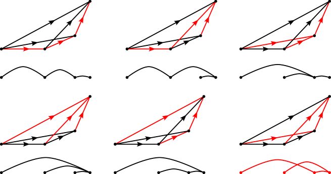
Figure 1. Tetrahedron with orientations induced by a generic objective function. The six possible $c$-arborescences are shown in red together with a simpler depiction as maps $\mathcal{A}:[3]\to[4]$ below. The bottom-right arborescence is not max-slope.

Definition 3.1 (Noncrossing arborescence).

An arborescence $\mathcal{A}:[n-1]\to[n]$ is noncrossing if $\mathcal{A}(j)\leq\mathcal{A}(i)$ for all $1\leq i<j<n$ with $j<\mathcal{A}(i)$.

In other words, $\mathcal{A}$ is noncrossing if there are no $a<i<b<j$ such that $\mathcal{A}(a)=b$ and $\mathcal{A}(i)=j$:

Theorem 3.2.

Let $\mathcal{A}:[n-1]\to[n]$ be an arborescence. Then $\mathcal{A}$ is a max-slope arborescence for $(\Delta_{n-1},c)$ if and only if $\mathcal{A}$ is noncrossing.

For the proof, we use a canonical decomposition of noncrossing arborescences; see Figure 2.

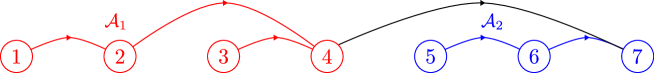
Figure 2. A noncrossing arborescence on $7$ nodes. $r=4$ is minimal with $\mathcal{A}(r)=7$. The decomposition into $\mathcal{A}_{1},\mathcal{A}_{2}$ is obtained by restricting to $1,\dots,4$ and $5,\dots,7$. The nodes $1,3,5$ are leaves and they are all immediate leaves.

Lemma 3.3.

Let $\mathcal{A}:[n-1]\to[n]$ be a noncrossing arborescence on $n\geq 2$ nodes. Let $r$ be minimal with $\mathcal{A}(r)=n$. Then $\mathcal{A}_{1}:[r-1]\to[r]$ given by $\mathcal{A}_{1}(i):=\mathcal{A}(i)$ for $i<r$ and $\mathcal{A}_{2}:[n-r-1]\to[n-r]$ given by $\mathcal{A}_{2}(i):=\mathcal{A}(r+i)-r$ are noncrossing arborescences. Moreover, $\mathcal{A}$ is uniquely determined by $(\mathcal{A}_{1},\mathcal{A}_{2})$.

3.3 allows us to count noncrossing arborescences. Recall that the famous Catalan numbers $C_{k}$ are given by $C_{0}:=1$ and

$$C_{k+1}\ :=\ C_{0}C_{k}+C_{1}C_{k-1}+\cdots+C_{k-1}C_{1}+C_{k}C_{0}$$ (3)

for $k\geq 0$; see also [16]. 3.3 shows that noncrossing arborescence $\mathcal{A}$ on $n$ nodes are in bijection with pairs of noncrossing arborescences $(\mathcal{A}_{1},\mathcal{A}_{2})$ of sizes $r$ and $n-r$, respectively, for $r=1,\dots,n-1$. We will make the connection to Catalan combinatorics more explicit when we describe the combinatorial structure of $\Pi(\Delta_{n-1},c)$. For now we record:

Corollary 3.4.

There are exactly $C_{n}$ many noncrossing arborescences on $n+1\geq 1$ nodes.

In light of 3.2 and the previous result, this shows that there are $C_{n}=\frac{1}{n+1}\binom{2n}{n}\sim 4^{n}/\sqrt{n^{3}\pi}$ many max-slope arborescences of an $n$-dimensional simplex, which has $n+1$ vertices and $\frac{n^{2}+n}{2}$ edges.

We call $k<n$ a leaf of $\mathcal{A}$ if there is no $i$ with $\mathcal{A}(i)=k$.

Lemma 3.5.

Let $\mathcal{A}$ be a noncrossing arborescence on $n\geq 2$ nodes. Then there is a leaf $k$ with $\mathcal{A}(k)=k+1$.

We call such a leaf an immediate leaf of $\mathcal{A}$.

Proof.

If $n=2$, then $\mathcal{A}=\{(1,2)\}$ and $1$ is an immediate leaf. For $n\geq 3$, let $(\mathcal{A}_{1},\mathcal{A}_{2})$ be the decomposition of $\mathcal{A}$ of 3.3. By induction $\mathcal{A}_{1}$ or $\mathcal{A}_{2}$ has an immediate leaf. ∎

For a fixed $w\in\mathbb{R}^{n}$, we define the slope of $1\leq i<j\leq n$ by

$$\tau({i,j})\ :=\ \frac{w_{j}-w_{i}}{c_{j}-c_{i}}\,.$$

Then $\mathcal{A}:[n-1]\to[n]$ is a max-slope arborescence with respect to $w$ if and only if for all $1\leq i<n$

$$\tau({i,\mathcal{A}(i)})\ >\ \tau({i,k})\quad\text{ for all }k>i\text{ and }k\neq\mathcal{A}(i)\,.$$ (4)

We will need the following convexity result.

Lemma 3.6.

For $1\leq r<s<t\leq n$ we have

$$\tau({r,t})>\tau({r,s})\ \Longleftrightarrow\ \tau({s,t})>\tau({r,t})\quad\text{ and }\quad\tau({r,t})<\tau({r,s})\ \Longleftrightarrow\ \tau({s,t})<\tau({r,t}).$$

Proof.

Note that

$$\tau({r,t})\ =\ \frac{c_{s}-c_{r}}{c_{t}-c_{r}}\tau({r,s})+\frac{c_{t}-c_{s}}{c_{t}-c_{r}}\tau({s,t})\,,$$

which implies $\max(\tau({r,s}),\tau({s,t}))\geq\tau({r,t})\geq\min(\tau({r,s}),\tau({s,t}))$. If $\tau({r,s})\neq\tau({s,t})$, then the inequalities are strict. ∎

Proof of 3.2.

Let $w\in\mathbb{R}^{n}$ be a weight such that $\mathcal{A}$ is the max-slope arborescence with respect to $w$. Assume that there are $1\leq a<i<b<j\leq n$ such that $(a,b)$ and $(i,j)$ are crossing arcs of $\mathcal{A}$. We claim that the following inequalities hold

$$\tau({i,b})\ <\ \tau({i,j})\ <\ \tau({b,j})\ <\ \tau({a,j})\ <\ \tau({a,b})\,.$$

The first and last inequality follow from (4) and the fact that $\mathcal{A}(i)=j$ and $\mathcal{A}(a)=b$. The second and third inequality follow from 3.6 for $i<b<j$ and $a<b<j$, respectively. In particular, we have $\tau({a,b})>\tau({i,b})$. On the other hand $\mathcal{A}(a)=b$ implies $\tau({a,b})>\tau({a,i})$ and 3.6 gives $\tau({i,b})>\tau({a,b})$. This is a contradiction.

Now let $\mathcal{A}$ be a noncrossing arborescence on $n$ nodes and recall that $c_{1}<\cdots<c_{n}$. We show the existence of a suitable $w=(w_{1},\dots,w_{n})$ by induction on the number of nodes $n$. Using (4), we need to verify that for every $1\leq i<k\leq n$ with $k\neq\mathcal{A}(i)$

$$0\ <(c_{k}-c_{i})w_{\mathcal{A}(i)}-(c_{\mathcal{A}(i)}-c_{i})w_{k}+(c_{\mathcal{A}(i)}-c_{k})w_{i}\ =:\ L_{i,k}(w)\,.$$

For $n\leq 2$, these conditions are vacuous. For $n>2$, let $l$ be an immediate leaf, whose existence is guaranteed by 3.5. We claim that the coefficient of $w_{l}$ in every inequality $L_{i,k}(w)>0$ is nonpositive. Since $l$ is leaf, there is no $i$ with $\mathcal{A}(i)=l$ and $w_{l}$ only occurs in inequalities $L_{i,k}(w)>0$ with $i=l$ or $k=l$. For $i<k=l$, the claim is clearly true. For $l=i<k$, the fact that $l$ is an immediate leaf and hence $\mathcal{A}(l)=l+1$ shows that $k>l+1$ and thus $c_{\mathcal{A}(l)}-c_{k}<0$. This means that the inequalities that involve $w_{l}$ only give upper bounds on $w_{l}$ in terms of the other $w_{i}$. The remaining inequalities determine the coherence of the arborescence $\overline{\mathcal{A}}$ obtained by restricting $\mathcal{A}$ to $[n]\setminus l$. Since $\overline{\mathcal{A}}$ is noncrossing on $n-1$ nodes, this system of strict inequalities is feasible by induction and we find a suitable $w_{l}$ satisfying the inequalities involving $l$. ∎

3.6 gives a simple criterion for finding an immediate leaf given a generic $w$. Define the maximal slope at $1\leq i<n$ by $\tau(i):=\max\{\tau(i,j):j>i\}$.

Corollary 3.7.

Let $w\in\mathbb{R}^{n}$ and $\mathcal{A}^{w}$ the max-slope arborescence for $(\Delta_{n-1},c)$. If $\tau(i)\geq\tau(k)$ for all $k$, then $i$ is an immediate leaf of $\mathcal{A}^{w}$.

Proof.

Assume that $\mathcal{A}(i)=j>i+1$, then $\tau(i,j)>\tau(i,i+1)$ and 3.6 implies $\tau(i+1,j)>\tau(i,j)$, which contradicts the maximality of $\tau(i)$. Hence $j=i+1$. Assume that there is $h<i$ with $\mathcal{A}^{w}(h)=i$. Then $\tau(h,i)>\tau(h,i+1)$ and again by 3.6 $\tau(h,i+1)>\tau(i,i+1)=\tau(i)$, which again contradicts maximality. ∎

4. Particles with locations and velocities

Consider $n\geq 2$ labelled particles on the real line. Every particle $i=1,2,\dots,n$ has a constant velocity $-c_{i}<0$. We assume that the velocities are distinct and, up to relabelling particles, satisfy $0<c_{1}<c_{2}<\cdots<c_{n}$. The velocities are fixed throughout. Assume further that at time $t=0$, the particles are at locations $-w_{1}\leq-w_{2}\leq\cdots\leq-w_{n}$. Figure 3 illustrates the setup.

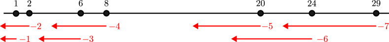
Figure 3. Locations (in black) $-w=(1,2,6,8,20,24,29)$ and velocities (in red) $-c=(-1,-2,-3,-4,-5,-6,-7)$ that produce the collision pattern of Figure 2.

Once the particles start moving from their initial locations $-w=(-w_{1},\dots,-w_{n})$ with velocities $-c=(-c_{1},\dots,-c_{n})$, they will eventually collide and merge. If particles $i<j$ collide, then particle $i$ is absorbed by the faster particle $j$, which continues at velocity $-c_{j}$. For $t\gg 0$, the only remaining particle is $n$; see Figure 4.

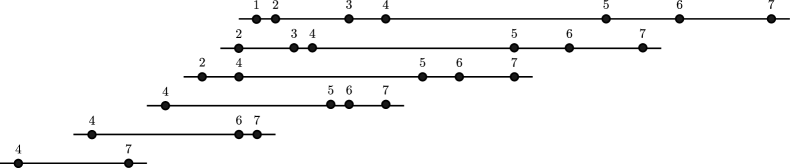
Figure 4. Shows the evolution of the particles of Figure 3 over time.

For now we assume that the locations $-w$ are chosen generically, so that at most two particles collide at any given point in time. We record the collisions by a map $\widetilde{\mathcal{A}}^{-w}:[n-1]\to[n]$ that we call a collision pattern: If particle $i$ gets absorbed by particle $j$ for the initial locations $-w$, then we set $\widetilde{\mathcal{A}}^{-w}(i):=j$. The connection to max-slope arborescences of simplices is as follows.

Theorem 4.1.

Let $n\geq 2$ and $c\in\mathbb{R}^{n}$ with $0<c_{1}<\cdots<c_{n}$. For $\mathcal{A}:[n-1]\to[n]$ and $w\in\mathbb{R}^{n}$, the following are equivalent.

1. $\mathcal{A}=\widetilde{\mathcal{A}}^{-(w-\alpha c)}$ is a collision pattern for $n$ particles with velocities $-c$ and locations $-(w-\alpha c)$ for some $\alpha\geq 0$.

2. $\mathcal{A}=\mathcal{A}^{w}$ is a max-slope arborescence of $(\Delta_{n-1},c)$ with respect to weight $w$.

Proof.

Let us first assume that $-w_{1}<\cdots<-w_{n}$. If we fix $j>i$ and disregard all other particles for the moment, then the time $t_{ij}$ of collision of $i$ and $j$ satisfies

$$-w_{i}-t_{ij}c_{i}\ =\ -w_{j}-t_{ij}c_{j}\qquad\Longleftrightarrow\qquad t_{ij}\ =\ \frac{-(w_{j}-w_{i})}{c_{j}-c_{i}}\,.$$ (5)

By construction, $i$ will be absorbed by particle $j$ if $t_{ij}$ is minimal among all $t_{ik}$ with $k>i$. Thus, for $i<n$, we observe

$$\widetilde{\mathcal{A}}^{-w}(i)\ =\ \operatorname{argmin}\left\{\frac{-(w_{j}-w_{i})}{c_{j}-c_{i}}:j>i\right\}\ =\ \operatorname{argmax}\left\{\frac{w_{j}-w_{i}}{c_{j}-c_{i}}:j>i\right\}\ =\ \mathcal{A}^{w}(i)\,,$$ (6)

where the last equation is the definition of $\mathcal{A}^{w}$ in (1). This proves the equivalence for strictly increasing $-w$. Note that both sides of (6) are invariant under replacing $w$ by $w-\alpha c$ for any $\alpha\in\mathbb{R}$. For $\alpha\geq 0$ sufficiently large, $-(w-\alpha c)$ is strictly increasing and thus satisfies our conditions on particle locations. ∎

The proof of 4.1 emphasizes that for any $w\in\mathbb{R}^{n}$, there is an $\alpha\geq 0$ such that $-(w-\alpha c)$ is strictly increasing and the associated collision pattern is independent of the choice of $\alpha$. Therefore, we will use noncrossing arborescence and collision plan interchangeably and will exclusively use the notation $\mathcal{A}^{w}$.

In the language of collision patterns, we can also interpret the decomposition of 3.3. If $\mathcal{A}^{w}$ is the collision pattern obtained from locations $-w$, then there is a time $t_{1}$ at which there are only two particles left. One of these two particles is clearly $n$, the other is the last particle that is absorbed by $n$, that is, the minimal $r\geq 1$ with $\mathcal{A}^{w}(r)=n$. In the time between $t=0$ and $t=t_{1}$, the particles $1,\dots,r-1$ get absorbed by $r$ and the particles $r+1,\dots,n-1$ get absorbed by $n$. The corresponding collision patterns are precisely $\mathcal{A}_{1}$ and $\mathcal{A}_{2}$, respectively.

The particle perspective also allows us to give an interpretation of the support function of $\Pi(\Delta_{n-1},c)$. For given weakly increasing $-w$, the lifespan of a particle $i<n$ is the timespan until it is absorbed by some particle $j>i$.

Proposition 4.2.

For $-w$ weakly increasing, $-h_{\Pi(\Delta_{n-1},c)}(w)$ is the sum of lifespans of all particles $i=1,\dots,n-1$.

Proof.

We compute

$$h_{\Pi(\Delta_{n-1},c)}(w)=\max_{\mathcal{A}}\langle{w,\psi(\mathcal{A})}\rangle=-\min_{\mathcal{A}}\langle{-w,\psi(\mathcal{A})}\rangle=-\min_{\mathcal{A}}\sum_{i<n}\frac{-(w_{\mathcal{A}(i)}-w_{i})}{c_{\mathcal{A}(i)}-c_{i}}=-\sum_{i<n}\min_{j>i}\frac{-(w_{j}-w_{i})}{c_{j}-c_{i}}$$

and thus $-h_{\Pi(\Delta_{n-1},c)}(w)$ is the sum of lifespans of all particles $i<n$. ∎

Collisions of particles can be encoded in terms of bracketings. A bracket is a subset of $[n]$ of the form $[i,j]:=\{i,i+1,\dots,j\}$ for $i\leq j$. A bracketing $\mathcal{B}$ is a collection of distinct brackets $B_{1},\dots,B_{m}$ such that for every $1\leq r<s\leq m$, $B_{r}\subset B_{s}$ or $B_{s}\subset B_{r}$ or $B_{s}\cap B_{r}=\varnothing$. A bracket represents particles that have collided with each other at some point in time. If $B_{r}\subset B_{s}$ are contained in a bracketing $\mathcal{B}$, then this means at some point all the particles in $B_{r}$ have collided and later all the particles in $B_{s}$ will have collided. As there is ultimately only a single particle left, every bracketing has to contain $[1,n]$. When convenient, we will also assume that $\mathcal{B}$ contains all singleton brackets $[i,i]$. The associahedron $\mathrm{Asso}_{n-2}$ is the set of bracketings of $[n]$ ordered by reverse inclusion. The unique maximal element is $\{[1,n]\}$. The minimal elements are the complete bracketings of $[n]$, that is, bracketings with $n-1$ brackets. Figure 5 gives an example.

Figure 5. The $\Pi(\Delta_{3},c)$ is combinatorially isomorphic to $\mathrm{Asso}_{2}$, which is a pentagon. The figure shows the corresponding labelling.

Theorem 4.3.

Let $P$ be an $(n-1)$-dimensional simplex and $c$ a generic objective function. Then $\Pi(P,c)$ is combinatorially isomorphic to the $(n-2)$-dimensional associahedron $\mathrm{Asso}_{n-2}$.

As a first step towards proving 4.3, we translate collision patterns into complete bracketings. Figure 6 illustrates the correspondence.

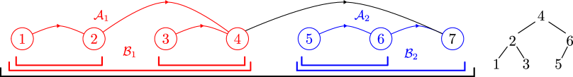
Figure 6. Left: the arborescence of Figure 2 together with the associated bracketing. Right: the associated partial order.

Theorem 4.4.

Collision patterns on $n$ particles are in bijection with complete bracketings.

Proof.

For $n\leq 2$, there is only one collision pattern and one complete bracketing. Let $\mathcal{A}$ be a collision pattern on $n>2$ particles. Let $\mathcal{A}_{1}:[r-1]\to[r]$ and $\mathcal{A}_{2}:[n-r-1]\to[n-r]$ be the decomposition of 3.3. By induction, $\mathcal{A}_{1},\mathcal{A}_{2}$ give rise to bracketings $\mathcal{B}_{1},\mathcal{B}_{2}$ on $r$ and $n-r$ particles, respectively. After the particles in $\mathcal{B}_{2}$ are relabelled from $[n-r]$ to $\{r+1,\dots,n\}$, we get a complete bracketing $\mathcal{B}=\mathcal{B}_{1}\cup\mathcal{B}_{2}\cup\{[1,n]\}$.

Conversely, if $\mathcal{B}$ is a complete bracketing, then $\mathcal{B}\setminus\{[1,n]\}$ decomposes into two complete bracketings $\mathcal{B}_{1},\mathcal{B}_{2}$ of $[1,r]$ and $[r+1,n]$. By induction they give rise to noncrossing arborescences $\mathcal{A}_{1},\mathcal{A}_{2}$ and 3.3 completes the proof. ∎

For the next result it will be convenient to extend the definition of collision patterns by setting $\mathcal{A}(0):=n$.

Lemma 4.5.

Let $\mathcal{A}$ be a collision pattern with associated bracketing $\mathcal{B}$. The bracket $[a,b]$ is contained in $\mathcal{B}$ if and only if $\mathcal{A}(a-1)\geq b$ and $\mathcal{A}^{k}(a)=b$ for some $k\geq 1$.

Proof.

Assume that $[a,b]\in\mathcal{B}$ and let $r$ be minimal with $\mathcal{A}(r)=n$. Unless $[a,b]=[1,n]$, $[a,b]\in\mathcal{B}_{1}$ or $[a,b]\in\mathcal{B}_{2}$, where $\mathcal{B}=\mathcal{B}_{1}\cup\mathcal{B}_{2}\cup\{[1,n]\}$ is the decomposition of the proof of 4.4. By induction, we can assume that $[a,b]=[1,r]$ or $[a,b]=[r+1,n]$. In the former, $r$ is the sink of $\mathcal{A}_{1}$ and hence $\mathcal{A}^{k}(1)=r$ for some $k$ and $\mathcal{A}(0)=n\geq r$. In the latter case, $n$ is the unique sink of $\mathcal{A}$ and $\mathcal{A}((r+1)-1)=n$.

Conversely, let $a<b$ with $\mathcal{A}(a-1)\geq b$ and $\mathcal{A}^{k}(a)=b$ for some $k\geq 1$. If $[a,b]=[1,n]$, then $[a,b]\in\mathcal{B}$. Otherwise, let $r\geq 1$ be minimal with $\mathcal{A}(r)=n$. Since $\mathcal{A}(a-1)\geq b$, noncrossing implies $1\leq r\leq a$ or $r\geq\mathcal{A}(a-1)\geq b$. If $r=a$, then this implies $b=n$. If $1\leq a-1$ or $r\geq\mathcal{A}(a-1)\geq b$, then we can replace $\mathcal{A}$ with $\mathcal{A}_{1}$ or $\mathcal{A}_{2}$, respectively and the claim follows by induction. ∎

We note that every weakly decreasing set of locations $w\in\mathbb{R}^{n}$ yields a partial bracketing. For example, as we saw earlier, $-w\in\mathbb{R}_{\geq 0}c+\mathbb{R}\mathbf{1}$ yields the coarsest bracketing $\mathcal{B}=\{[1,n]\}$. This point of view allows us to explicitly construct locations for single brackets.

Proposition 4.6.

Let $1\leq r<s\leq n$ with $(r,s)\neq(1,n)$. The bracketing $\mathcal{B}=\{[r,s],[1,n]\}$ is obtained from locations $-w$ if and only if

$$-\mu w+\gamma\mathbf{1}-\alpha c\ =\ -w^{r,s}\ :=\ (c_{1},\dots,c_{r-1},c_{s},\dots,c_{s},c_{s+1},\dots,c_{n})$$

for some $\gamma,\alpha,\mu\in\mathbb{R}$ with $\alpha\geq 0$ and $\mu>0$. Moreover, $-h_{\Pi(\Delta_{n-1},c)}(w^{r,s})=n-1-(s-r)$.

Proof.

If $-w$ yields the bracketing $\{[r,s],[1,n]\}$, then there are exactly two points in time $t_{1}<t_{2}$ when collisions happen. At time $t_{1}$, the particles $[r,s]$ simultaneously collide and at $t_{2}$, all the remaining particles $1,\dots,r-1,s,s+1,\dots,n$ simultaneously collide. Using 2.3, we can replace $-w$ by $-w^{\prime}=\frac{1}{t_{2}-t_{1}}(-w-t_{1}c)$ and assume that $t_{1}=0$ and $t_{2}=1$. Hence $-w^{\prime}$ satisfies $w^{\prime}_{r}=\cdots=w^{\prime}_{s}$ and $w^{\prime}_{i}-c_{i}=\gamma$ for some $\gamma$ and all $i<r$ and $i\geq s$. As for the sum of lifespans with respect to locations $-w^{r,s}$, we note that particles $r,\dots,s-1$ have lifespan $0$ and particles $i<r$ and $s\leq i<n$ have lifespan $1$. Thus $-h_{\Pi(\Delta_{n-1},c)}(w^{r,s})=n-1-(s-r)$ by 4.2. ∎

Note that the faces described in 4.6 have a unique normal relative to the affine hull of $\Pi(\Delta_{n-1},c)$ and hence are facets. We write $[a,b]^{c}$ for the complement $[n]\setminus[a,b]$.

Proposition 4.7.

Let $\mathcal{A}$ be a collision pattern and $1\leq r<s\leq n$ with $(r,s)\neq(1,n)$. Then $\psi(\mathcal{A})$ is contained in the face $\Pi(\Delta_{n-1},c)\cap\{x:\langle{-w^{r,s},x}\rangle=n-1-(s-r)\}$ if and only if $\mathcal{A}$ maps $[r,s-1]$ into $[r,s]$ and $[r,s-1]^{c}$ into $[r,s-1]^{c}$.

Proof.

Since $-w^{r,s}$ is weakly increasing, we get from 4.6 that $\langle{-w^{r,s},\psi(\mathcal{A})}\rangle\geq n-1-(s-r)$. Equality holds if and only if $\frac{-(w^{r,s}_{\mathcal{A}(i)}-w^{r,s}_{i})}{c_{\mathcal{A}(i)}-c_{i}}$ is minimal for all $i<n$. For $i<r$, this is the case if $\mathcal{A}(i)<r$ or $\mathcal{A}(i)\geq s$, in which case the value is $1$. For $r\leq i<s$, the minimal value $0$ is attained if and only if $\mathcal{A}(i)\leq s$. ∎

Bracketings that contain of a single bracket $[r.s]\neq[1,n]$ correspond to the facets of any polytopal realization of $\mathrm{Asso}_{n-2}$. 4.6 shows that $\Pi(\Delta_{n-1},c)$ has a unique facet for every such bracketing. 4.7 gives a combinatorial characterization of which vertices are contained in those facets and is a decisive step in showing that $\mathrm{Asso}_{n-2}$ and $\Pi(\Delta_{n-1},c)$ have the same vertex-facet incidences. However at this point, we cannot exclude that $\Pi(\Delta_{n-1},c)$ has more facets. For that, we need the following general result.

Lemma 4.8.

Let $P$ and $Q$ be two polytopes of the same dimension. Assume that $f:V(P)\to V(Q)$ is a bijection on vertices such that for every facet $F\subset P$, there is a face $G\subset Q$ with $f(V(F))=V(G)$. Then $P$ and $Q$ are combinatorially isomorphic.

Proof.

Every face is uniquely identified by its set of vertices and we can view the face lattice $L(P)=\{V(F):F\subseteq P\text{ face}\}$ as a subposet of $2^{V(P)}$. Since every face is an intersection of facets, $f$ extends to an injective map $f:L(P)\to L(Q)$. Therefore, we can view $L(P)$ as a graded sublattice of $L(Q)$. Since both polytopes have the same dimension, it follows that $f(F)$ is a facet of $Q$ for all facets $F\subset P$. Assume that there is a facet of $Q$ not contained in $L(P)$. The dual graph of $Q$ is connected and thus there exists a facet $G\in L(Q)\setminus L(P)$ and a facet $F\in L(P)$ such that $\dim F\cap G=\dim P-2=\dim Q-2$. However, since $L(P)$ is the face lattice of a polytope and $F$ is a facet, there is a unique facet $F^{\prime}\in L(P)$ with $F\cap G=F\cap F^{\prime}$. Since $F^{\prime}$ is also a facet of $Q$, this implies $G=F^{\prime}$. ∎

Proof of 4.3.

Using 2.3 we can assume that $P=\Delta_{n-1}$ and $0<c_{1}<\cdots<c_{n}$.

Let $\mathcal{A}$ be a collision pattern with bracketing $\mathcal{B}$ and $1\leq r<s\leq n$ with $[r,s]\neq[1,n]$. We first prove that $\psi(\mathcal{A})$ is contained in the face $\Pi(\Delta_{n-1},c)^{w^{r,s}}$ if and only if $[r,s]\in\mathcal{B}$. From 4.7 we get that $\psi(\mathcal{A})\in\Pi(\Delta_{n-1},c)^{w^{r,s}}$ if and only if $\mathcal{A}([r,s-1])\subseteq[r,s]$ and $\mathcal{A}([r,s-1]^{c})\subseteq[r,s]^{c}$. If $\mathcal{A}([r,s-1])\subseteq[r,s]$, then there is some $k$ such that $\mathcal{A}^{k}(r)=s$. Moreover, if $\mathcal{A}([r,s-1]^{c})\subseteq[r,s]^{c}$, then $\mathcal{A}(r-1)\geq s$. 4.5 now implies that $[r,s]\in\mathcal{B}$. Conversely, if $\mathcal{A}$ satisfies $\mathcal{A}(r-1)\geq s$ then $\mathcal{A}(i)\in[1,r-1]\cup[s,n]$ for all $1\leq i\leq r-1$. Since trivially $\mathcal{A}([s,n])\subseteq[s+1,n]$, this shows $\mathcal{A}([r,s-1]^{c})\subseteq[r,s]^{c}$. If there is $i\in[r,s-1]$ with $\mathcal{A}(i)>s$, then there is no $k$ such that $\mathcal{A}^{k}(r)=s$. Hence, $\mathcal{A}([r,s-1])\subseteq[r,s]$, which proves the claim.

By 4.4, we have a bijection $f$ from complete bracketings to collision patterns, that is, vertices of $\Pi(\Delta_{n-1},c)$. The facets of $\mathrm{Asso}_{n-2}$, that is, the maximal elements of $\mathrm{Asso}_{n-2}$ correspond to the bracketings $\{[r,s],[1,n]\}$ with $1\leq r<s\leq n$ and $(r,s)\neq(1,n)$. The claim above now states $[r,s]\in\mathcal{B}$ if and only if $\psi(f(\mathcal{B}))\in\Pi(\Delta_{n-1},c)^{w^{r,s}}$. Finally, $\mathrm{Asso}_{n-2}$ is the face lattice of a polytope of dimension $d-2=\dim\Pi(\Delta_{n-1},c)$ and 4.8 completes the proof. ∎

Remark 4.9.

A simpler proof of 4.3 proceeds as follows. From the proof of 3.2 is it not difficult to determine when $[\psi(\mathcal{A}),\psi(\mathcal{A}^{\prime})]$ is an edge of $\Pi(\Delta_{n-1},c)$. In particular, one sees that the graph of $\Pi(\Delta_{n-1},c)$ is $(d-2)$-regular and hence $\Pi(\Delta_{n-1},c)$ is a simple polytope. Blind and Mani [3] showed that two simple polytopes are combinatorially isomorphic if and only if they have isomorphic graphs; see also [19, Sect. 3.4]. 4.4 actually gives an isomorphism of graphs and completes the argument. However, the pivot rule polytopes of products of simplices are not simple and the correspondence to constrainahedra will need a similar argument.

In the next section, we need yet another representation of particle collisions. For a collision pattern $\mathcal{A}$, we define a partial order by setting $i\prec j$ if particle $i$ has to be absorbed before particle $j$ can be absorbed. Since the particle $n$ is never absorbed, this is a partial order on $[n-1]$. For example, in the collision pattern of Figure 6, we note that $3$ needs to be absorbed by $4$ before $2$ can be absorbed. However, since $2$ absorbs $1$, this has to happen before $2$ can absorbed by $4$. Hence $1\prec 2$ and $3\prec 2$. There is no dependence between $1$ and $3$ and they are not comparable with respect to $\preceq$. The complete partial order is shown in Figure 6.

It is straightforward to see that $i$ is a minimal element with respect to $\preceq$ if and only if $i$ is an immediate leaf. Moreover, there is a unique element $j$ that covers $i$, that is, $i\prec j$ and there is no $j^{\prime}$ with $i\prec j^{\prime}\prec j$. Let $j$ be the maximal $k<i$ with $\mathcal{A}(k)=\mathcal{A}(i)$. If such a $j$ exists, the noncrossing condition demands $j=i-1$. By removing $i$ from the collision pattern (and relabelling), we see that $j$ becomes an immediate leaf and that $i$ was the only obstruction. If there is no $k<i$ with $\mathcal{A}(k)=\mathcal{A}(i)=i+1$, then $j=\mathcal{A}(i)=i+1$. Indeed, once all particles $j+1,\dots,\mathcal{A}(j)-1$ have been absorbed by $\mathcal{A}(j)$, $i$ is the only obstruction for $j$ becoming an immediate leaf. Observe that in the Hasse diagram of $\preceq$ every non-maximal element is covered by a unique element and every element covers at most two elements. The Hasse diagram is a binary search tree.

Lemma 4.10.

Let $\mathcal{A}$ be a collision pattern on $n\geq 2$ particles with associated partial order $\preceq$. For $a,b\in[n-1]$, we have $a\preceq b$ if and only if $a\leq b$ and $b=\mathcal{A}^{k}(a)$, or $b<a$ and $\mathcal{A}(b)=\mathcal{A}^{k+1}(a)$ for some $k\geq 0$.

Proof.

We prove the equivalence by induction on $n$. If $n=2$, then $a=b$ and the equivalence is trivially true. Assume that $n>2$ and $a\neq b$. By 3.5, $\mathcal{A}$ has an immediate leaf. Assume that there is an immediate leaf $c\not\in\{a,b\}$. As discussed before, $c$ is a minimum of $\preceq$ that can be removed without changing the order relation between $a$ and $b$. Similarly, $c$ can be removed from the collision pattern without interfering with the stated conditions. In this case, the equivalence holds by induction.

If no such $c$ exists, then $a$ or $b$ has to be the unique immediate leaf of $\mathcal{A}$. If $b$ is the immediate leaf then neither condition can hold. Thus $a$ is an immediate leaf and there is a unique $j$ that covers $a$. Removing $a$, we get by induction that $j\preceq b$ if and only if $j\leq b$ and there is $k\geq 0$ with $b=\mathcal{A}^{k}(j)$ or $j>b$ and $\mathcal{A}(b)=\mathcal{A}^{k}(j)$ for some $k>0$. By the preceding discussion, we have that $j=\mathcal{A}(a)$ or $\mathcal{A}(j)=\mathcal{A}(a)$. In the former case, we have $b=\mathcal{A}^{k}(j)$ if and only if $b=\mathcal{A}^{k+1}(a)$ and $\mathcal{A}(b)=\mathcal{A}^{k}(j)$ if and only if $\mathcal{A}(b)=\mathcal{A}^{k+1}(a)$. In the latter case, we have $b=\mathcal{A}^{k}(j)$ if and only if $b=\mathcal{A}^{k}(a)$ and $\mathcal{A}(b)=\mathcal{A}^{k}(j)$ if and only if $\mathcal{A}(b)=\mathcal{A}^{k}(a)$. ∎

5. Products of simplices and constrainahedra

In this section we investigate the max-slope pivot rule polytopes of the product of two simplices. As in the case of simplices, the construction of max-slope arborescences lends itself to an interpretation in terms of particle collisions.

Let $m,n\geq 1$ and consider the Cartesian product of an $(m-1)$-simplex and an $(n-1)$-simplex. Appealing to 2.3, it suffices to consider

$$P_{m-1,n-1}\ :=\ \Delta_{m-1}\times\Delta_{n-1}\ \subset\ \mathbb{R}^{m}\times\mathbb{R}^{n}\ \cong\ \mathbb{R}^{m+n}\,.$$

Let us write $e^{\prime}_{r}=e_{r}$ for $r=1,\dots,m$ and $e^{\prime\prime}_{i}=e_{m+i}$ for $i=1,\dots,n$. Then $P_{m-1,n-1}$ is a simple polytope with $m\cdot n$ vertices $e^{\prime}_{r}+e^{\prime\prime}_{i}$ for $r=1,\dots,m$ and $i=1,\dots,n$, contained in the codimension-$2$ subspace of all $(x^{\prime},x^{\prime\prime})\in\mathbb{R}^{m}\times\mathbb{R}^{n}$ with $\sum_{r}x^{\prime}_{r}=\sum_{i}x^{\prime\prime}_{i}=1$. We choose an edge-generic objective function $c=(c^{\prime},c^{\prime\prime})\in\mathbb{R}^{m}\times\mathbb{R}^{n}$, for which we can assume that $0<c^{\prime}_{1}<c^{\prime}_{2}<\cdots<c^{\prime}_{m}$ and $0<c^{\prime\prime}_{1}<c^{\prime\prime}_{2}<\cdots<c^{\prime\prime}_{n}$. The graph of $P_{m-1,n-1}$ oriented by $c$ has nodes $V_{m,n}:=[m]\times[n]$ that we write as $ri$ for $r\in[m]$ and $i\in[n]$ and edges of the form $ri\to rj$ for $i<j$ (vertical edges) and $ri\to si$ for $r<s$ (horizontal edges). The unique sink is the node $mn$ and we write $V^{\circ}_{m,n}:=V_{m,n}\setminus\{mn\}$.

Arborescences of $(P_{m-1,n-1},c)$ can be identified with maps $\mathcal{A}:V^{\circ}_{m,n}\to V_{m,n}$ with the property that if $\mathcal{A}(ri)=sj$ then $r<s$ and $i=j$ or $r=s$ and $i<j$. The number of arborescences is $\prod_{i=1}^{m-1}\prod_{j=1}^{n-1}(i+j)$. Every arborescence $\mathcal{A}$ determines an arborescence $\mathcal{A}^{\prime}$ of $(\Delta_{m-1},c^{\prime})$ by $\mathcal{A}^{\prime}(r):=s$ if $\mathcal{A}(rn)=sn$. Analogously, we obtain an arborescence $\mathcal{A}^{\prime\prime}$ for $(\Delta_{n-1},c^{\prime\prime})$.

Let $w=(w^{\prime},w^{\prime\prime})\in\mathbb{R}^{m}\times\mathbb{R}^{n}$ be generic. In order to determine the max-slope arborescence of $P_{m-1,n-1}$ with respect to $w$, let $\mathcal{A}^{w^{\prime}}:[m-1]\to[m]$ be the max-slope arborescence of $(\Delta_{m-1},c^{\prime})$ determined by $w^{\prime}$. If $\mathcal{A}^{w^{\prime}}(r)=s$, then $s$ maximizes the slope $\tau^{\prime}(r,s)=\frac{w^{\prime}_{s}-w^{\prime}_{r}}{c^{\prime}_{s}-c^{\prime}_{r}}$ and we record the maximal slope at $r$ as $\tau^{\prime}(r):=\tau^{\prime}(r,s)$. Likewise, $\mathcal{A}^{w^{\prime\prime}}$ is the max-slope determined by $w^{\prime\prime}$ and we define $\tau^{\prime\prime}$ analogously. Evaluating (1), we see that the max-slope $\mathcal{A}^{w}$ on $(P_{m-1,n-1},c)$ is given by

$$\mathcal{A}^{w}(ri)\ =\ \begin{cases}\mathcal{A}^{w^{\prime}}(r)i&\text{if }\tau^{\prime}(r)>\tau^{\prime\prime}(i)\\ r\mathcal{A}^{w^{\prime\prime}}(i)&\text{if }\tau^{\prime}(r)<\tau^{\prime\prime}(i).\\ \end{cases}$$ (7)

Figure 7 shows an example.

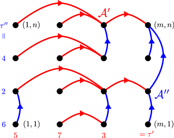
Figure 7. Example of a max-slope arborescence $\mathcal{A}^{w}$ for $(P_{m-1,n-1},c)$ with $(m,n)=(4,4)$, $c^{\prime}=(1,2,3,4)$, and $c^{\prime\prime}=(5,6,7,8)$. The weights are $w^{\prime}=(11,14,21,24)$ and $w^{\prime\prime}=(38,44,44,48)$. The slopes $\tau^{\prime}(r)$ and $\tau^{\prime\prime}(i)$ are indicated below.

In order to describe them combinatorially, we make the following definitions. A node $ri\in V_{m,n}$ is an immediate leaf of $\mathcal{A}$ if it has no incoming edges and $\mathcal{A}(ri)=(r+1)i$ or $\mathcal{A}(ri)=r(i+1)$.

Definition 5.1.

For $m,n\geq 1$ an arborescence $\mathcal{A}:V^{\circ}_{m,n}\to V_{m,n}$ is reducible if $m=n=1$ or

• there exists $r\in[m]$ such that $ri$ is a immediate leaf for every $i$ and the restriction of $\mathcal{A}$ to $V^{\circ}_{m,n}\setminus(r\times[n])$ is reducible, or

• there exists $i\in[n]$ such that $ri$ is a immediate leaf for every $r$ and the restriction of $\mathcal{A}$ to $V^{\circ}_{m,n}\setminus([m]\times i)$ is reducible.

Figure 8 shows that the arborescence in Figure 7 is reducible. The existence of rows or columns of immediate leaves is the key property for many of the arguments in this section. Note that Lemma 3.5 shows that noncrossing arborescences are reducible. In fact, the next observation shows that being noncrossing is a consequence of reducibility. Let $\mathcal{A}:V^{\circ}_{m,n}\to V_{m,n}$ be a reducible arborescence and recall that $\mathcal{A}$ induces arborescences $\mathcal{A}^{\prime}$ and $\mathcal{A}^{\prime\prime}$ on $(\Delta_{m-1},c^{\prime})$ and $(\Delta_{n-1},c^{\prime\prime})$, respectively. We call $\mathcal{A}$ consistent if $\mathcal{A}(ri)=si$ implies $\mathcal{A}^{\prime}(r)=s$ and $\mathcal{A}(ri)=rj$ implies $\mathcal{A}^{\prime\prime}(i)=j$ for all $ri\in V^{\circ}_{m,n}$. We call $\mathcal{A}$ grid-noncrossing if $\mathcal{A}^{\prime}$ and $\mathcal{A}^{\prime\prime}$ are noncrossing and there are no $1\leq r\leq s<t\leq m$ and $1\leq i\leq j<k\leq n$ with $(r,i)\neq(s,j)$ and with $\mathcal{A}(si)=sk$ and $\mathcal{A}(rj)=tj$. We can illustrate an arborescence $\mathcal{A}:V^{\circ}_{m,n}\to V_{m,n}$ as in Figure 7 by drawing arcs horizontally or vertically between consecutive rows or columns of nodes. Consistency now means that every arc is a copy of the top-most horizontal arc in the same column or right-most vertical arc in the same row. Grid-noncrossing states that every row and column is a partial noncrossing arborescence and there are is no crossing of a vertical and a horizontal arc.

Proposition 5.2.

If $\mathcal{A}$ is reducible, then $\mathcal{A}$ is consistent and grid-noncrossing.

Proof.

We prove the claim by induction on $m+n$. If $m=n=1$, this is trivial. For $m+n>0$, we can remove a row or column of immediate leafs. Both claims hold by induction and bringing back the row or column keeps both properties intact. ∎

For $m=1$ or $n=1$, reducible arborescences are precisely the noncrossing arborescences. Figure 9 shows 5.2 does not give an equivalence. It would be interesting to have a non-recursive characterization of reducible arborescences. The combinatorial notion of reducibility suffices to completely characterize max-slope arborescences of products of two simplices.

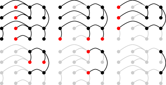
Figure 8. The figure shows that the arborescence of Figure 7 is reducible. The red nodes correspond to rows or columns of immediate leaves.

Figure 9. An example of a consistent and grid-noncrossing arborescence that is not reducible.

Theorem 5.3.

An arborescence $\mathcal{A}:V^{\circ}_{m,n}\to V_{m,n}$ is a max-slope arborescence of $(P_{m-1,n-1},c)$ if and only if $\mathcal{A}$ is reducible.

Proof.

Let $\mathcal{A}=\mathcal{A}^{w}$ be a max-slope arborescence for some $w=(w^{\prime},w^{\prime\prime})$. We show by induction on $m+n$ that $\mathcal{A}^{w}$ is reducible. The base case $m=n=1$ is trivially true. Let $r$ with $\tau^{\prime}(r)$ maximal and $i$ with $\tau^{\prime\prime}(i)$ maximal. Without loss of generality, let us assume that $\tau^{\prime}(r)>\tau^{\prime\prime}(i)$. From 3.7 we know that $r$ is an immediate leaf of $\mathcal{A}^{\prime}$ and there are no horizontal arcs into $rj$ for all $j$. Moreover, (7) shows that $\mathcal{A}(rj)=(r+1)j$ for all $j$. This shows that $rj$ is an immediate leaf for all $j$. We also note that the restriction of $\mathcal{A}^{w}$ to $V^{\circ}_{m,n}\setminus r\times[n]$ is the max-slope arborescence of $P_{m-2,n-1}$ for $\hat{c}=(c^{\prime}_{1},\dots,c^{\prime}_{r-1},c^{\prime}_{r+1},\dots,c^{\prime}_{m},c^{\prime\prime})$ and $w=(w^{\prime}_{1},\dots,w^{\prime}_{r-1},w^{\prime}_{r+1},\dots,w^{\prime}_{m},w^{\prime\prime})$. The claim follows by induction.

To prove the converse, let $\mathcal{A}:V^{\circ}_{m,n}\to V_{m,n}$ be a reducible arborescence. We prove the existence of $w=(w^{\prime},w^{\prime\prime})\in\mathbb{R}^{m+n}$ by induction on $(m,n)$. If $m=1$ or $n=1$, then $\mathcal{A}$ is a noncrossing arborescence and the claim reduces to 3.2. Thus, let $m>1$ and $n>1$. By reducibility and without loss of generality, we may assume that $ri$ is an immediate leaf of $\mathcal{A}$ for all $i$. The restriction of $\mathcal{A}$ to $r\times[n]$ is a reducible arborescence for $(P_{m-2,n-1},\hat{c})$ with $\hat{c}$ as above and by induction there is a suitable $\hat{w}=(w^{\prime}_{1},\dots,w^{\prime}_{r-1},w^{\prime}_{r+1},\dots,w^{\prime}_{m},w^{\prime\prime}_{1},\dots,w^{\prime\prime}_{n})$ that proves that the restriction is a max-slope arborescence. In order to find $w^{\prime}_{r}$, we obtain from the proof of 3.2, that the inequalities $L_{rs}(w^{\prime})>0$ with $r<s$ pose only upper bounds on $w^{\prime}_{r}$. In particular, we can choose $w^{\prime}_{r}$ such that $\tau^{\prime}(r)>\tau^{\prime}(s)$ for $s\neq r$. Similarly, let $i\in[n]$ with $\tau^{\prime\prime}(i)$ maximal. The condition $\tau^{\prime}(r)>\tau^{\prime\prime}(i)$ is again an upper bound on $w^{\prime}_{r}$. Thus for $w^{\prime}_{r}$ sufficiently small, $\mathcal{A}=\mathcal{A}^{w}$ for $w=(w^{\prime},w^{\prime\prime})$. ∎

To view max-slope arborescences of $P_{m-1,n-1}$ as particle collisions, we use the following generalization of particles on a line due by Bottman and Poliakova [5]. We consider $m$ vertical lines $L^{\prime}_{1},\dots,L^{\prime}_{m}$ and $n$ horizontal lines $L^{\prime\prime}_{1},\dots,L^{\prime\prime}_{n}$. The lines are labelled left-to-right and bottom-to-top. We place a particle $ri$ at the point of intersection of $L^{\prime}_{r}$ and $L^{\prime\prime}_{i}$. The particle movements are induced by parallel displacements of the $m+n$ lines. In this scenario parallel lines collide and particles contained in the colliding lines merge.

We equip every line $L^{\prime}_{r}$ and $L^{\prime\prime}_{i}$ with a location $-w^{\prime}_{r}$ and $-w^{\prime\prime}_{i}$ at time $t=0$ and we assume that $-w^{\prime}_{1}\leq-w^{\prime}_{2}\leq\cdots\leq-w^{\prime}_{m}$ and $-w^{\prime\prime}_{1}\leq-w^{\prime\prime}_{2}\leq\cdots\leq-w^{\prime\prime}_{n}$. For $t>0$, the lines $L^{\prime}_{r}$ move to the left with constant velocity $-c^{\prime}_{r}$, the lines $L^{\prime\prime}_{i}$ move down with constant velocity $-c^{\prime\prime}_{i}$. As before we assume that $0<c^{\prime}_{1}<c^{\prime}_{2}<\cdots<c^{\prime}_{m}$ and $0<c^{\prime\prime}_{1}<c^{\prime\prime}_{2}<\cdots<c^{\prime\prime}_{n}$. If two or more lines collide, they are absorbed by the line with the largest index and this line continues at its original speed. If we assume that the locations $-w=(-w^{\prime},-w^{\prime})$ are sufficiently generic, then no more than two lines collide and we can encode the collisions of particles by a collision pattern $\widetilde{\mathcal{A}}^{-w}:V^{\circ}_{m,n}\to V_{m,n}$; see Figure 10 for an illustration.

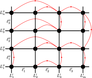
Figure 10. The figure shows the $m=4$ vertical lines $L^{\prime}_{r}$ and the $n=4$ horizontal lines $L^{\prime\prime}_{i}$ together with the $16$ particles at the intersections and the collision pattern from Figure 7.

The same argument as for 4.1 yields the following.

Theorem 5.4.

Let $m,n\geq 2$ and $c=(c^{\prime},c^{\prime\prime})\in\mathbb{R}^{m+n}$ with $0<c^{\prime}_{1}<c^{\prime}_{2}<\cdots<c^{\prime}_{m}$ and $0<c^{\prime\prime}_{1}<c^{\prime\prime}_{2}<\cdots<c^{\prime\prime}_{n}$. For $\mathcal{A}:V^{\circ}_{m,n}\to V_{m,n}$ and $w=(w^{\prime},w^{\prime\prime})\in\mathbb{R}^{m+n}$, the following are equivalent:

1. $\mathcal{A}=\widetilde{\mathcal{A}}^{-(w-\alpha c)}$ is a collision pattern for $m\cdot n$ particles contained in $m$ vertical lines and $n$ horizontal lines moving at velocities $c=(-c^{\prime},-c^{\prime\prime})$ and starting at locations $-(w-\alpha c)$ for some $\alpha\geq 0$.

2. $\mathcal{A}=\mathcal{A}^{w}$ is a max-slope arborescence of $(P_{m-1,n-1},c)$ with respect to weight $w$.

The combinatorics of collisions of $m\cdot n$ particles sitting on $m$ vertical and $n$ horizontal lines was modelled in [5] by certain preorders on $\mathcal{L}=\{L^{\prime}_{1},\dots,L^{\prime}_{m-1},L^{\prime\prime}_{1},\dots,L^{\prime\prime}_{n-1}\}$. Recall that a preorder on $\mathcal{L}$ is a reflexive and transitive relation $\preceq$. For $x\in\mathcal{L}$, the equivalence class $[x]$ is the collection of elements $y\in\mathcal{L}$ with $x\preceq y$ and $y\preceq x$. On the collection of equivalence classes $\preceq$ yields a partial order. Bottman and Poliakova define a preorder $\preceq$ on $\mathcal{L}$ to be a good rectangular preorder [5, Def. 2.1] if

• $L^{\prime}_{r}$ and $L^{\prime\prime}_{i}$ are comparable for all $r,i$ (orthogonal comparability)

and $L^{\prime}_{o}\preceq L^{\prime}_{q}$ (respectively $L^{\prime\prime}_{o}\preceq L^{\prime\prime}_{q}$) if and only if

• $L^{\prime}_{o}\preceq L^{\prime\prime}_{p}\preceq L^{\prime}_{q}$ (respectively $L^{\prime\prime}_{o}\preceq L^{\prime}_{p}\preceq L^{\prime\prime}_{q}$) for some $p$, or (orthogonal link)

• there is no $\min(o,q)<p<\max(o,q)$ with $L^{\prime}_{o}\prec L^{\prime}_{p}\succ L^{\prime}_{q}$ (respectively $L^{\prime\prime}_{o}\prec L^{\prime\prime}_{p}\succ L^{\prime\prime}_{q}$). (no gaps)

From a collision pattern $\mathcal{A}$, we construct a partial order $\preceq$ on $\mathcal{L}$ that captures which lines have to be absorbed before other lines can be absorbed. The lines $L^{\prime}_{m}$ and $L^{\prime\prime}_{n}$ are never absorbed. Let $\preceq^{\prime}$ and $\preceq^{\prime\prime}$ be the partial orders on $L^{\prime}_{1},\dots,L^{\prime}_{m-1}$ and $L^{\prime\prime}_{1},\dots,L^{\prime\prime}_{n-1}$ obtained from $\mathcal{A}^{\prime}$ and $\mathcal{A}^{\prime\prime}$, respectively; cf. 4.10 and the discussion preceding it. We define the binary relation $\preceq$ by

1. $L^{\prime}_{r}\preceq L^{\prime\prime}_{i}$ if $\mathcal{A}(ri)=si$ and $L^{\prime\prime}_{i}\preceq L^{\prime}_{r}$ if $\mathcal{A}(ri)=rj$;

2. $L^{\prime}_{r}\preceq L^{\prime}_{s}$ if $L^{\prime}_{r}\preceq^{\prime}L^{\prime}_{s}$ or $L^{\prime}_{r}\preceq L^{\prime\prime}_{i}\preceq L^{\prime}_{s}$ for some $i$;

3. $L^{\prime\prime}_{i}\preceq L^{\prime\prime}_{j}$ if $L^{\prime\prime}_{i}\preceq^{\prime\prime}L^{\prime\prime}_{j}$ or $L^{\prime\prime}_{i}\preceq L^{\prime}_{r}\preceq L^{\prime\prime}_{j}$ for some $r$.

Proposition 5.5.

The binary relation $\preceq$ is a good rectangular partial order on $\mathcal{L}$.

Proof.

We first prove that $\preceq$ is a partial order. By reducibility, let us assume that $ri$ is an immediate leaf for all $i$. This implies that $L^{\prime}_{r}\prec L^{\prime\prime}_{i}$ for all $i$. Moreover, $r$ is an immediate leaf of $\mathcal{A}^{\prime}$ and hence $L^{\prime}_{r}$ is a minimum with respect to $\preceq^{\prime}$. This implies that if $x\preceq L^{\prime}_{r}$ then $x=L^{\prime}_{r}$. By induction, this shows that $\preceq$ restricted to $\mathcal{L}\setminus\{L^{\prime}_{r}\}$ is a partial order and that $\preceq$ is reflexive and anti-symmetric on $\mathcal{L}$. We are left to show that if $L^{\prime}_{r}\prec x$ and $x\prec y$, then $L^{\prime}_{r}\prec y$. If there is some $L^{\prime\prime}_{i}$ with $x\preceq L^{\prime\prime}_{i}\preceq y$, then we are done. Hence $x=L^{\prime}_{s}$ and $y=L^{\prime}_{t}$ for some $s,t$ and $L^{\prime}_{s}\prec^{\prime}L^{\prime}_{t}$. Since $\preceq^{\prime}$ is transitive, we get $L^{\prime}_{r}\preceq^{\prime}L^{\prime}_{t}$ and hence $L^{\prime}_{r}\preceq L^{\prime}_{t}$.

To show that $\preceq$ is good rectangular, we only need to show that the no gaps condition characterizes $\preceq^{\prime}$ (and hence $\preceq^{\prime\prime}$). Assume that $1\leq r<s<t\leq m-1$. From 4.10 we get that $L^{\prime}_{r}\prec L^{\prime}_{s}$ if and only if $s=(\mathcal{A}^{\prime})^{k}(r)$ for some $k>0$ and $L^{\prime}_{t}\prec L^{\prime}_{s}$ if and only if $\mathcal{A}^{\prime}(s)=(\mathcal{A}^{\prime})^{l}(t)$ for some $l>0$. There is no $h$ with $t=(\mathcal{A}^{\prime})^{h}(r)$ and since $\mathcal{A}(r)\leq s$, there is no $h$ with $(\mathcal{A}^{\prime})^{h}(t)=\mathcal{A}(r)$. Thus $L^{\prime}_{r}$ and $L^{\prime}_{t}$ are incomparable. The converse argument is analogous. ∎

5.5 gives a way to build up the partial order by successively removing rows or columns of immediate leaves. Figure 11 gives an example. Note that the Hasse diagram is not a tree anymore. Removing a row/column of immediate leaves might open up rows/columns of immediate leaves.

Figure 11. A collision pattern and the corresponding poset.

5.5 shows that the partial order associated to a collision pattern is a good rectangular poset. In fact, every good rectangular poset arises that way.

Proposition 5.6.

Collision patterns for $m$ vertical and $n$ horizontal lines are in bijection with good rectangular posets.

Proof.

This follows by reducibility and induction on $m+n$. ∎

A good rectangular preorder $\preceq_{2}$ is refined by $\preceq_{1}$ if $x\preceq_{1}y$ implies $x\preceq_{2}y$ for all $x,y\in\mathcal{L}$.

Theorem 5.7 ([5, Theorem 4.1]).

The good rectangular preorders on $\mathcal{L}=\{L^{\prime}_{1},\dots,L^{\prime}_{m-1},L^{\prime\prime}_{1},\dots,L^{\prime\prime}_{n-1}\}$ partially ordered by refinement is the face poset of an $(m+n-3)$-dimensional polytope and is called the $(m,n)$-constrainahedron $C(m,n)$.

In the rest of this section we will prove the following.

Theorem 5.8.

For $m,n\geq 2$ and a generic $c\in\mathbb{R}^{m+n}$, the max-slope pivot polytope $\Pi(P_{m-1,n-1},c)$ is combinatorially isomorphic to the $(m,n)$-constrainahedron.

Let us call a simultaneous collision of horizontal and vertical lines an elementary collision if it is not the result of at least two simultaneous and disjoint collisions of sets of lines. These elementary collisions come in three types for which we give locations for fixed velocities $c=(c^{\prime},c^{\prime\prime})\in\mathbb{R}^{m+n}$:

1. For $1\leq r\leq t\leq m-1$, the vertical lines $M=\{L^{\prime}_{s}:r\leq s\leq t\}$ are simultaneously absorbed followed by the simultaneous collision of all vertical and horizontal lines $\mathcal{L}\setminus M$. Note that the lines in $M$ are absorbed by $L^{\prime}_{t+1}$. The corresponding good rectangular preorder has equivalence classes $M$ and $\mathcal{L}\setminus M$.

   We define $-w^{\mathrm{VC}}_{r,t}:=(w^{\prime},c^{\prime\prime})$ where $w^{\prime}_{s}:=c^{\prime}_{t+1}$ if $s\in[r,t]$ and $w^{\prime}_{s}:=c^{\prime}_{s}$ otherwise. The total lifespan is $-h_{\Pi(P_{m-1,n-1},c)}(w^{\mathrm{VC}}_{r,s})=(n-1)(m-1-(t-r))$.

2. For $1\leq i\leq k\leq n-1$, the horizontal lines $M=\{L^{\prime\prime}_{j}:i\leq j\leq k\}$ are simultaneously absorbed (by $L^{\prime\prime}_{k+1}$) followed by the simultaneous collision of all vertical and horizontal lines $\mathcal{L}\setminus M$. The corresponding good rectangular preorder has equivalence classes $M$ and $\mathcal{L}\setminus M$.

   We define $-w^{\mathrm{HC}}_{i,k}:=(c^{\prime},w^{\prime\prime})$ where $w^{\prime\prime}_{j}:=c^{\prime\prime}_{k+1}$ if $j\in[i,k]$ and $w^{\prime\prime}_{j}:=c^{\prime\prime}_{j}$ otherwise. The total lifespan is $-h_{\Pi(P_{m-1,n-1},c)}(w^{\mathrm{HC}}_{i,k})=(m-1)(n-1-(k-i))$.

For the last type of elementary collisions, let us call a non-empty collection of intervals $\mathcal{I}=\{I_{1},\dots,I_{g}\}$ of $[k]$ discontinuous if they are pairwise disjoint and $I_{i}\cup I_{j}$ is not an interval for $i\neq j$. We write $\bigcup\mathcal{I}=I_{1}\cup\cdots\cup I_{g}$.

1. Let $\mathcal{I}^{\prime}$ and $\mathcal{I}^{\prime\prime}$ be discontinuous collections of $[m-1]$ and $[n-1]$, respectively, such that $\mathcal{I}^{\prime}\neq\{[m-1]\}$ or $\mathcal{I}^{\prime\prime}\neq\{[n-1]\}$. The collection of lines $M=\{L^{\prime}_{r},L^{\prime\prime}_{i}:r\in\bigcup\mathcal{I}^{\prime},i\in\bigcup\mathcal{I}^{\prime\prime}\}$ are simultaneously absorbed followed by the simultaneous collision of all lines $\mathcal{L}\setminus M$.

   We define $-w^{\mathrm{MC}}_{\mathcal{I}^{\prime},\mathcal{I}^{\prime\prime}}:=(w^{\prime},w^{\prime\prime})$ where $w^{\prime}_{s}:=c^{\prime}_{t+1}$ if $s\in[r,t]\in\mathcal{I}^{\prime}$ and $w^{\prime}_{s}:=c^{\prime}_{s}$ otherwise and $w^{\prime\prime}_{j}:=c^{\prime\prime}_{k+1}$ if $j\in[i,k]\in\mathcal{I}^{\prime\prime}$ and $w^{\prime\prime}_{j}:=c^{\prime}_{j}$ otherwise. The total lifespan is $-h_{\Pi(P_{m-1,n-1},c)}(w^{\mathrm{HC}}_{i,k})=(m-1)(n-1)-|\bigcup\mathcal{I}^{\prime}|\cdot|\bigcup\mathcal{I}^{\prime\prime}|$.

Proof of 5.8.

The proof follows the same strategy as the proof of 3.2. By 5.6, there is a bijection between good rectangular orders $\preceq$ in $C(m,n)$ and the vertices of $\Pi(P_{m-1,n-1},c)$, that is, reducible arborescences $\mathcal{A}:V^{\circ}_{m,n}\to V_{m,n}$. Let $\sqsubseteq$ be a coarsest nontrivial good rectangular preorder in $C(m,n)$. We show that there is a face $F\subset\Pi(P_{m-1,n-1},c)$ such that $\preceq$ refines $\sqsubseteq$ if and only if $\psi(\mathcal{A})\in F$. Since $\Pi(P_{m-1,n-1},c)$ and $C(m,n)$ are polytopes of dimension $m+n-3$, 4.8 yields the claim. For $m=1$ or $n=1$, this is precisely the proof of 3.2.

Following [5], the coarsest good rectangular preorders are those associated to elementary collisions of types (VC), (HC), and (MC). Let us assume that $\sqsubseteq$ represents an elementary collision of type (VC) with $M=\{L^{\prime}_{s}:r\leq s\leq t\}$ for some $1\leq r\leq t\leq m-1$. The two other cases are treated analogously. Let $-w=-w^{\mathrm{VC}}_{r,s}$ be the locations realizing the elementary collision and let $F=\Pi(P_{m-1,n-1},c)^{-w}$. For these locations, we have $\tau^{\prime\prime}(j)=-1$ for all $j\in[n]$ and $\tau^{\prime}(q)=0$ if $q\in[r,t]$ and $\tau^{\prime}(q)<0$ otherwise. In particular, $\psi(\mathcal{A})$ is contained in $F$ if and only if $\mathcal{A}$ has a total lifespan $\langle{-w,\psi(\mathcal{A})}\rangle$ of $(n-1)(m-1-(t-r))$.

We will use the fact that if $x\in\mathcal{L}$ is minimal with respect to $\preceq$, then $\preceq$ refines $\sqsubseteq$ if and only if $x\in M$ and $\preceq$ refines $\sqsubseteq$ when restricted to $\mathcal{L}\setminus x$.

Assume that $\preceq$ refines $\sqsubseteq$. If $x$ is minimal with respect to $\preceq$, then $x$ corresponds to a row or column of immediate leaves of $\mathcal{A}$. Now $x\in M$ implies $x=L^{\prime}_{s}$ for some $s\in[r,t]$ and thus $\mathcal{A}(si)=(s+1)i$ for all $i$. In particular, $\tau^{\prime}(s)=0$ and hence this row of immediate leaves contributes $0$ to the total live span $\langle{-w,\psi(\mathcal{A})}\rangle$. That is $\langle{-w,e^{\prime}_{s+1}-e^{\prime}_{s}}\rangle=0$ and comparing with (2), we see that deleting the $s$-th coordinate of $\psi(\mathcal{A})-(n-1)\frac{e^{\prime}_{s+1}-e^{\prime}_{s}}{c^{\prime}_{s+1}-c^{\prime}_{s}}$ is precisely $\psi(\overline{\mathcal{A}})$, where $\overline{\mathcal{A}}$ is the restriction of $\mathcal{A}$ to $V^{\circ}_{m,n}\setminus s\times[n]$. If we now set $\overline{w}=(w^{\prime}_{1},\dots,w^{\prime}_{s-1},w^{\prime}_{s+1},\dots,w^{\prime}_{m},w^{\prime\prime})\in\mathbb{R}^{m-1+n}$, then $\psi(\mathcal{A})\in F=\Pi(P_{m-1,n-1},c)^{-w}$ if and only if $\psi(\overline{\mathcal{A}})\in\Pi(P_{m-2,n-1},c)^{-\overline{w}}$ and the proof follows by induction.

For the converse, let $\psi(\mathcal{A})$ be a vertex of $F=\Pi(P_{m-1,n-1},c)^{-w}$. In particular, there is $\widetilde{w}\in\mathbb{R}^{m+n}$ such that $\mathcal{A}$ is the max-slope arborescence with respect to $\widetilde{w}$. For every $\varepsilon>0$, $\mathcal{A}=\mathcal{A}^{w+\varepsilon\widetilde{w}}$. For $\varepsilon$ sufficiently small, we gather from (7) that a minimum $x$ of $\preceq$ corresponds to a row of immediate leaves $\mathcal{A}(si)=(s+1)i$ for $s\in[r,t]$ and $i=1,\dots,n-1$. Hence $x=L^{\prime}_{s}\in M$. The same argument as above shows that $\psi(\mathcal{A})-(n-1)\frac{e^{\prime}_{s+1}-e^{\prime}_{s}}{c^{\prime}_{s+1}-c^{\prime}_{s}}$ descents to a vertex of $\Pi(P_{m-2,n-1},c)^{-\overline{w}}$ and we are done by induction. ∎

6. Higher products and multiplihedra

The particle interpretations of the previous section generalize to max-slope pivot rule polytopes of higher products of simplices

$$P_{n_{1},\dots,n_{k}}\ :=\ \Delta_{n_{1}}\times\cdots\times\Delta_{n_{k}}\,,$$

by considering collections of hyperplanes parallel to the coordinate planes in $\mathbb{R}^{k}$ and with particles sitting at their $0$-dimensional intersections.

If $n_{i}=1$ for all $i=1,\dots,k$, then $P$ is linearly isomorphic to a $k$-dimensional cube and the max-slope pivot rule polytope was determined in [2]. Let $\mathfrak{S}_{k}$ be the permutations of $[k]$. Recall that the permutahedron $\Pi(a_{1},\dots,a_{k})$ for $a_{1},\dots,a_{k}\in\mathbb{R}$ is the convex hull of $(a_{\sigma(1)},\dots,a_{\sigma(k)})$ for for all $\sigma\in\mathfrak{S}_{k}$. If all $a_{i}$ are distinct, then $\Pi(a_{1},\dots,a_{k})$ is a simple $(k-1)$-dimensional polytope with $k!$ many vertices; cf. [19, Section 0].

Proposition 6.1 ([2, Example 4.2]).

If $n_{1}=\cdots=n_{k}=1$, then the max-slope pivot rule polytope of $P_{n_{1},\dots,n_{k}}$ is linearly isomorphic to the permutahedron $\Pi(2^{0},2^{1},\dots,2^{k-1})$.

This agrees with the particle perspective, where we would consider for each $i=1,\dots,k$ two hyperplanes in $\mathbb{R}^{k}$ parallel to $\{x_{i}=0\}$. Collisions here correspond to the event that two parallel hyperplanes meet and hence the relevant information is the order in which these events take place.

In this last section, we focus on the max-slope pivot rule polytopes of $P_{n-1,1,1,\dots,1}=\Delta_{n-1}\times(\Delta_{1})^{k}$. Making use of 2.3, it suffices to look at the polytopes

$$Q_{n,k}\ :=\ \Delta_{n-1}\times[0,1]^{k}\ \subset\ \mathbb{R}^{n}\times\mathbb{R}^{k}\,$$

together with an objective function $(c,r)\in\mathbb{R}^{n+k}$ with $c=(c_{1}<c_{2}<\cdots<c_{n})$ and $r=(r_{1},\dots,r_{k})\in\mathbb{R}^{k}$ with $r_{i}>0$ for all $i$. The vertices of $Q_{n,k}$ can be identified with pairs $(i,B)$ with $i\in[n]$ and $B\subseteq[k]$. There is a directed edge from $(i,B)$ to $(j,C)$ if and only if $i<j$ and $B=C$ or $i=j$ and $C=B\cup\{b\}$ for some $b\in[k]\setminus B$. In particular the unique sink is $(n,[k])$.

Theorem 6.2.

Let $(\mathbb{A},\cdot)$ be a non-associative monoid and let $f_{1},\dots,f_{k}:\mathbb{A}\to\mathbb{A}$ be morphisms. The vertices of $\Pi(Q_{n,k},(c,r))$ are in bijection with the possible ways of evaluating

$$(f_{\sigma(1)}\circ f_{\sigma(2)}\circ\cdots\circ f_{\sigma(k)})(a_{1}\cdot a_{2}\cdots a_{n})\,,$$

where $a_{1},\dots,a_{n}\in\mathbb{A}$ and $\sigma\in\mathfrak{S}_{k}$ is a permutation.

For $k\geq 2$, all polytopes $\Pi(Q_{n,k},(c,r))$ of dimension $\leq 3$ are permutahedra. Figure 12 gives an illustration for $n=k=2$. Note that if $k=0$, then $Q_{n,0}=\Delta_{n-1}$ and $\Pi(Q_{n,k},(c,r))$ is the associahedron by 4.3. For $k=1$, 6.2 yields that the vertices of $\Pi(\Delta_{n-1}\times\Delta_{1},(c,r))$ are in bijection with the vertices of Stasheff’s multiplihedron; see [17]. Indeed, $\Pi(\Delta_{n-1}\times\Delta_{1},(c,r))$ is the constrainahedron $C(2,n)=C(n,2)$ by 5.8, which coincides with the multiplihedron by [5, Theorem 2.1]. 6.2 insinuates that $\Pi(Q_{n,k},(c,r))$ is combinatorially isomorphic to the $(k,n)$-multiplihedron of Chapoton–Pilaud [7]. Germain Poullot found a general piecewise-linear connection between max-slope pivot rule polytopes of products of simplices and shuffle products of associahedra; see [14, Section 3.2].

Figure 12. An illustration of the $(2,2)$-multiplihedron.

Consider an evaluation of $(f_{\sigma(1)}\circ f_{\sigma(2)}\circ\cdots\circ f_{\sigma(k)})(a_{1}\cdot a_{2}\cdots a_{n})$ with $\sigma$ fixed. Disregarding the morphisms for a moment, the order in which the $n-1$ multiplications have to be carried out is encoded by a partial order $\preceq_{T}$ on $[n-1]$ whose Hasse diagram is well-known to be a tree $T$ rooted at the maximum (i.e., the last multiplication to be carried out). Every node in the tree has at most two children. With the labelling given by $[n-1]$, the possible posets are precisely the binary search trees on $n-1$ nodes. Now, for the $j$-th multiplication, we record the number $\phi(j)$ of morphisms that have to be applied before the multiplication can take place. The poset $([n-1],\preceq_{T})$ together with the map $\phi:[n-1]\to\{0,1,\dots,k\}$ completely determines the evaluation. Note that if $i\prec j$, then $\phi(i)\leq\phi(j)$ and hence $\phi$ is an order-preserving map.

Let $(w,s)\in\mathbb{R}^{n+k}$ be a generic weight. As before, we define $\tau(i,j):=\frac{w_{j}-w_{i}}{c_{j}-c_{i}}$ for $1\leq i<j\leq n$ and $\tau(i)=\max_{j>i}\tau(i,j)$. By genericity we can assume that $s_{g}\neq s_{h}$ for $g\neq h$. Let $(i,B)\neq(n,[k])$ and let $h\in[k]\setminus B$ such that $s_{h}$ is maximal. Unravelling (1) we find that

$$\mathcal{A}^{(w,s)}(i,B)\ =\ \begin{cases}(\mathcal{A}^{w}(i),B)&\text{ if }\tau(i)>s_{h}\\ (i,B\cup\{h\})&\text{ if }\tau(i)<s_{h}.\end{cases}$$

There is unique permutation $\sigma\in\mathfrak{S}_{k}$ such that $s_{\sigma(1)}>s_{\sigma(2)}>\cdots>s_{\sigma(k)}$. Moreover, for every $i\in[n-1]$, define $\phi_{s}(i):=|\{h\in[k]:\tau(i)>s_{h}\}|$. Then the arborescence $\mathcal{A}^{w,s}$ is completely determined by $(\tau,\sigma,\phi_{s})$.

Recall from 4.10 that any noncrossing arborescence $\mathcal{A}:[n-1]\to[n]$ determines a partial order $\preceq$ on $[n-1]$ whose Hasse diagram is given by a binary search tree on $[n-1]$.

Lemma 6.3.

For a generic weight $w\in\mathbb{R}^{n}$ let $([n-1],\preceq)$ be the poset associated to the noncrossing arborescence $\mathcal{A}^{w}$. If $a\prec b$, then $\tau(a)>\tau(b)$.

Proof.

It suffices to assume that $a$ is covered by $b$, that is, $a\prec b$ and there is no $s$ such that $a\prec s\prec b$. It follows from 4.10 that this is the case if $a=b-1$ and $\mathcal{A}^{w}(a)=b$ or $a=b+1$ and $\mathcal{A}^{w}(a)=\mathcal{A}^{w}(b)=a+1$.

Let $c=\mathcal{A}^{w}(b)$ In the former case, 3.6 with $(r,s,t)=(a,b,c)$ implies $\tau(a)=\tau(a,b)>\tau(a,c)>\tau(b,c)=\tau(b)$. In the latter case when $b<a$, $\tau(b)=\tau(b,c)>\tau(b,a)$ and 3.6 with $(r,s,t)=(b,a,c)$ yields $\tau(b,c)<\tau(a,c)=\tau(a)$. ∎

Proof of 6.2.

Let $(w,s)$ be a generic weight. The noncrossing arborescence $\mathcal{A}^{w}$ determines a partial order $([n-1],\preceq)$ whose Hasse diagram is a binary search tree $T$. By 6.3, the map $\phi_{s}$ associated to $s$ is order-preserving and takes values in $\{0,1\dots,k\}$. Thus, together with the permutation $\sigma$, this uniquely determines a unique evaluation of $(f_{\sigma(1)}\circ f_{\sigma(2)}\circ\cdots\circ f_{\sigma(k)})(a_{1}\cdot a_{2}\cdots a_{n})$ as discussed above. Conversely, given such an evaluation represented by a permutation $\sigma$, a partial order $([n-1],\preceq)$, and an order-preserving map $\phi$, there is a unique noncrossing arborescence $\mathcal{A}$ which gives rise to $([n-1],\preceq)$. By 3.2, we can find $w\in\mathbb{R}^{n}$ with $\mathcal{A}=\mathcal{A}^{w}$. Finally, given $\sigma$ and $\phi$, we can find numbers $s_{1},\dots,s_{k}$ with $s_{\sigma(i)}>s_{\sigma(i+1)}$ and $\phi(i)=\phi_{s}(i)$ for all $i=1,\dots,k$. ∎

The order polynomial $\Omega_{P}(l)$ of a partially ordered set $(P,\preceq)$ is a polynomial of degree $|P|$ such that $\Omega_{P}(l)$ is the number of order-preserving maps $P\to[l]$. The order polynomial was introduced by Stanley and is well-studied; see, for example, [15, 1]. For fixed $n\geq 2$, we define

$$V_{n}(k)\ :=\ \sum_{T}\Omega_{T}(k+1)\,,$$

where the sum is over all binary search trees $T$ of on $n$ nodes. Our encoding of an evaluation of $(f_{\sigma(1)}\circ f_{\sigma(2)}\circ\cdots\circ f_{\sigma(k)})(a_{1}\cdot a_{2}\cdots a_{n})$ by a binary search tree and an order-preserving map into $\{0,1,\dots,k\}$ yields the following.

Corollary 6.4.

The number of evaluations of $(f_{\sigma(1)}\circ f_{\sigma(2)}\circ\cdots\circ f_{\sigma(k)})(a_{1}\cdot a_{2}\cdots a_{n})$ is $V_{n}(k)$. In particular, the number of vertices of $\Pi(Q_{n,k},(c,r))$ is $k!V_{n}(k)$.

The number of vertices of the $(k,n)$-multiplihedron is given Proposition 126 of [7] as $k!$ times the coefficient of $y^{n+1}$ of the power series $C^{(m+1)}(y)$, where $C^{(1)}(y)=\frac{1-\sqrt{1-4y}}{2}$ is the Catalan generating function and $C^{(i+1)}(y)=C(C^{(i)}(y))$. It is remarkable that the number of vertices for varying $k$ is essentially given by a polynomial. The following table shows a few of the polynomials $V_{n}(k)$.

$$\begin{array}[]{l|l}n&V_{n}(k)\\ \hline\cr 2&k^{2}+3k+2\\ 3&k^{3}+\frac{11}{2}k^{2}+\frac{19}{2}k+5\\ 4&k^{4}+\frac{25}{3}k^{3}+25k^{2}+\frac{95}{3}k+14\\ 5&k^{5}+\frac{137}{12}k^{4}+\frac{101}{2}k^{3}+\frac{1291}{12}k^{2}+\frac{219}{2}k+42\\ 6&k^{6}+\frac{147}{10}k^{5}+\frac{263}{3}k^{4}+\frac{541}{2}k^{3}+\frac{1360}{3}k^{2}+\frac{1944}{5}k+132\\ 7&k^{7}+\frac{363}{20}k^{6}+\frac{2069}{15}k^{5}+\frac{6809}{12}k^{4}+\frac{8161}{6}k^{3}+\frac{56773}{30}k^{2}+\frac{14079}{10}k+429\\ 8&k^{8}+\frac{761}{35}k^{7}+\frac{36461}{180}k^{6}+\frac{63229}{60}k^{5}+\frac{60125}{18}k^{4}+\frac{395189}{60}k^{3}+\frac{1415369}{180}k^{2}+\frac{362247}{70}k+1430\\ 9&k^{9}+\frac{7129}{280}k^{8}+\frac{7915}{28}k^{7}+\frac{64549}{36}k^{6}+\frac{42877}{6}k^{5}+\frac{6665857}{360}k^{4}+\frac{373321}{12}k^{3}+\frac{8211733}{252}k^{2}+\frac{269403}{14}k+4862\\ \end{array}$$

As the table shows, all coefficients are non-negative and, of course, we tested if the polynomials are real-rooted. This seems to be true for $n\leq 10$ but unknown beyond. For $n\leq 10$, $(n-1)!V_{n}(k)$ has integer coefficients which are log-concave. We end with two simple observations regarding the polynomial.

Theorem 6.5.

For $n\geq 2$, the leading coefficient of $V_{n}(k)$ is $1$ and the constant coefficient is the $n$-th Catalan number $C_{n}$.

Proof.

For the constant coefficient, we simply note that $\Omega_{T}(1)=1$ and hence $V_{n}(0)$ is the number of trees $C_{n}$. For the leading coefficient, we recall that the leading coefficient of $n!\Omega_{T}(l)$ is the number of linear extensions $e(T)$ of $T$, that is, order-preserving bijections $\ell:T\to[n]$; see [1, Sect. 6.2]. If $\ell=(\ell_{1},\dots,\ell_{n})$ is a list of distinct numbers, there is a simple recursive procedure that produces a binary tree $T$ on nodes $1,\dots,n$ such that $i\mapsto\ell_{i}$ gives a order preserving map on $T$; see, for example, [18]. If $i$ is the index such that $\ell_{i}$ is maximal, then set $i$ to be the root of the binary tree. The left subtree is determined by $(\ell_{1},\dots,\ell_{i-1})$ and the right subtree is determined by $(\ell_{i+1},\dots,\ell_{n})$. Thus, every bijection $[n]\to[n]$ determines a unique binary tree $T$ and the number of bijections that produce $T$ is $e(T)$. Hence $\sum_{T}e(T)=n!$. ∎

References

[1]M. Beck and R. Sanyal, Combinatorial reciprocity theorems, vol. 195
of Graduate Studies in Mathematics, American Mathematical Society,
Providence, RI, 2018.
[2]A. E. Black, J. A. De Loera, N. Lütjeharms, and R. Sanyal, The
polyhedral geometry of pivot rules and monotone paths, SIAM Journal on
Applied Algebra and Geometry, 7 (2023), pp. 623–650.
[3]R. Blind and P. Mani-Levitska, Puzzles and polytope isomorphisms,
Aequationes Math., 34 (1987), pp. 287–297.
[4]N. Bottman, 2-associahedra, Algebr. Geom. Topol., 19 (2019),
pp. 743–806.
[5]N. Bottman and D. Poliakova, Constrainahedra.
August 2022,
arXiv:2208.14529.
[6]C. Ceballos, F. Santos, and G. M. Ziegler, Many non-equivalent
realizations of the associahedron, Combinatorica, 35 (2015), pp. 513–551.
[7]F. Chapoton and V. Pilaud, Shuffles of deformed permutahedra,
multiplihedra, constrainahedra, and biassociahedra.
January 2022,
arXiv:2201.06896.
[8]S. Forcey, Convex hull realizations of the multiplihedra, Topology
Appl., 156 (2008), pp. 326–347.
[9]S. Gass and T. Saaty, The computational algorithm for the parametric
objective function, Naval Res. Logist. Quart., 2 (1955), pp. 39–45.
[10]C. W. Lee, The associahedron and triangulations of the -gon,
European J. Combin., 10 (1989), pp. 551–560.
[11]V. Pilaud and D. Poliakova, Hochschild polytopes.
July 2023, arXiv:2307.05940.
[13]A. Postnikov, Permutohedra, associahedra, and beyond, International
Mathematics Research Notices, 2009 (2009), pp. 1026–1106.
[14]G. Poullot, Geometric combinatorics of paths and deformations of
convex polytopes, theses, Sorbonne Université, Oct. 2023.
[15]R. P. Stanley, Enumerative combinatorics. Volume 1, vol. 49 of
Cambridge Studies in Advanced Mathematics, Cambridge University Press,
Cambridge, second ed., 2012.
[16], Catalan numbers,
Cambridge University Press, New York, 2015.
[17]J. Stasheff, -spaces from a homotopy point of view, vol. Vol.
161 of Lecture Notes in Mathematics, Springer-Verlag, Berlin-New York, 1970.
[18]A. Tonks, Relating the associahedron and the permutohedron, in
Operads: Proceedings of Renaissance Conferences (Hartford,
CT/Luminy, 1995), vol. 202 of Contemp. Math., Amer. Math. Soc.,
Providence, RI, 1997, pp. 33–36.
[19]G. M. Ziegler, Lectures on polytopes, vol. 152, Springer Science &
Business Media, 2012.