A Survey on Complexity Measures for Pseudo-Random Sequences
Abstract
Since the introduction of the Kolmogorov complexity of binary sequences in the 1960s, there have been significant advancements in the topic of complexity measures for randomness assessment, which are of fundamental importance in theoretical computer science and of practical interest in cryptography. This survey reviews notable research from the past four decades on the linear, quadratic and maximum-order complexities of pseudo-random sequences and their relations with Lempel-Ziv complexity, expansion complexity, 2-adic complexity, and correlation measures.
Keywords Kolmogorov complexity; randomness; feedback shift register; linear complexity; nonlinear complexity; Lempel-Ziv complexity; expansion complexity; 2-adic complexity; correlation
1 Introduction
Consider a sequence of terms extracted from certain alphabet. Researches on the randomness of the sequence can be traced back to early 20th century. As early as in 1919 Mises [1] initiated the notion of random sequences based on his frequency theory of probability. Later Church [2] pointed out the vagueness of the second condition on randomness in [1] and proposed a less restricted but more precise definition of random sequences: an infinite binary sequence is a random sequence if it satisfies the following two condition: 1) if is the number of 1’s among the first terms of , then approaches a limit as approaches infinity; 2) if is any effectively calculable function of positive integers, if , and the integers such that form in order of magnitude an infinite sequence , and if is the number of 1’s among the first terms of , then approaches the same limit as approaches infinity. Despite the emphasis of calculability of in Condition 2), one can see that it is hardly (if not at all) possible to test the randomness of a sequence by this definition. It could be used in randomness test by negative outcomes, namely, a binary sequence is not random if one can find certain effectively calculable function , for which Condition 2) cannot hold. In order to justify a proposed definition of randomness, one has to show that the sequences, which are random in the stated sense, possess various properties of stochasticity with which we are acquainted in the theory of probability. Inspired by the properties obeyed by the maximum-length sequences, Golomb proposed the randomness postulates of binary sequences [3]: balancedness, run property111A subsequence of consecutive 1’s/0’s in a sequence is termed a run. A maximum-length sequence of length contains one run of 1’s, one run of 0’s and runs of 1’s and 0’s for . and ideal autocorrelation. Martin-Löf [4] and Kolmogorov [5] proposed the notion of complexity to test the randomness of a sequence with respect to certain algorithm (namely, universal Turing machine program), which is defined as , the length of the shortest that can produce by the algorithm . This complexity measure depends essentially on the algorithm in question. Along this line further developments were made in [6] and summarized in [7].
Rather than considering an abstract Turing machine program that generates a given sequence, the model of using feedback shift registers (FSRs) to generate a given sequence had attracted considerable attentions. This model has two major advantages: firstly, all sequences that are generated by a finite-state machine in a deterministic manner are ultimately periodic, and as such, can be produced by certain finite-state shift registers; secondly, it is comparatively easier and more efficient to identify the shortest FSRs producing a given sequence, either of a finite length or of infinite length with a certain period. Due to its tractability, linear complexity of a specific sequence , which uses linear FSRs as the algorithm , is particularly appealing and has been intensively studied. The linear complexity of a given sequence can be efficiently calculated by the Berlekamp-Massey algorithm [8, 9], and the stochastic behavior of linear complexity for finite-length sequences and periodic sequences can be considered to be fairly well understood [10, 11, 12]. The good understanding of linear complexity of random is an important factor for its adoption in the NIST randomness test suite [13]. Given (ultimately) periodic sequences, the Berlekamp-Massey can efficient find an LFSR generate them. However, for extremely long sequences with large linear complexity they can be generated by much short FSRs with nonlinear feedback functions or some other ways. More figures of merit to judge the randomness of sequences, such as maximum-order complexity [14], 2-adic complexity [15], quadratic complexity [16], expansion complexity [17] and their variants, have been also explored in the literature.
This paper will survey the development of complexity measures used to assess the randomness of sequences. It is important to note that this paper does not intend to offer a comprehensive survey of this broad topic. Instead it aims to provide a preliminary overview of the topic with technical discussions to certain extent, focusing on mainly complexities within the domain of FSR that align with the author’s research interests. To this end, we delved into significant findings on the study of FSR-based complexity measures, particularly on the algorithmic and algebraic methods in computation, statistical behavior, theoretical constructions, relations of those complexity measures. Research papers on this topic presented at flagship conferences in cryptography, such as CRYPTO and EUROCRYPT, published at prestigious journals with IEEE, Springer, Science Direct, etc, as well as some well-recognized books since 1970s contribute the major content of this survey. Readers may refer to relevant surveys on this topic with different focuses by Meidl and Niederreiter [Meidl2002a, 12], Topuzoǧlus and Winterhof [18].
The remainder of this paper is organized as follows: Section 2 defines notations, recalls the basics for feedback shift registers, which lays the foundation for the discussions in subsequent sections. Section 3 reviews important developments of the theory of linear complexity profile for random sequences and Section 4 discusses a mathematical tool used for efficiently calculate the quadratic complexity of sequences. In Section 5 we review computational methods and the statistical behavior for maximum-order complexity and discuss theoretical constructions of periodic sequences with largest maximum-order complexity. Section 6 briefly discusses known relations among complexity measures of sequences. Finally, conclusive remarks and discussion are given in Section 7.
2 Preliminary
Let be the finite field of elements, where is an arbitrary prime power. For a positive integer , an -stage feedback shift register (FSR) is a clock-controlled circuit consisting of consecutive storage units and a feedback function as displayed in Figure 1. Starting with an initial state over , the states in the FSR will be updated by a clock-controlled transformation as follows:
| (1) |
where
and the leftmost symbol for each state will be output. In this way an FSR produces a sequence based on each initial state and its feedback function .
For an -stage FSR with a feedback function and an initial state , if we know consecutive in the output , then we obtain equations
| (2) |
When the feedback function is a linear, i.e., , if , one can uniquely determine its unknown coefficients from the above linear equations by the Gaussian elimination. This process can be further improved by the Berlekamp-Massey algorithm [8, 9], which outputs the linear recurrence by evaluating the discrepancy of the existing linear recurrence on each new term. When the feedback function is nonlinear, the number of terms in increases significantly. For instance, for a binary feedback function of degree has possible terms. The above equations in (2) become more difficult to analyze. The equations are not necessarily linearly independent and a lot more variables are involved. Consequently, more observations and techniques are required in the analysis of these equations. In the following we will review some results on FSR sequences when the feedback function is linear, quadratic and arbitrarily nonlinear, and their relations with other complexity measures.
Any sequence generated by a finite-state machine will be ultimately repeating. Recall that a sequence is said to be -periodic if for any . In this case, is a period of but not necessarily the least period. In this paper we will only consider the least period of a periodic sequence and call it the period of the sequence as usual. We will consider both finite-length sequences and infinite-length sequences with certain finite period. Throughout what follows, we will use to denote a generic sequence with terms from certain alphabet, to denote a sequence with length that is not a repetition of any shorter sequence, to denote a sequence of repetition of and to denote infinite repetitions of the sequence .
3 Linear Complexity
Given an FSR, when its feedback function is a linear function on the input state, namely, it is associated with the following linear recurrence:
| (3) |
where are taken from , it is termed linear FSR and the output sequence is called an LFSR sequence of order . The polynomial
with , is called the feedback or characteristic polynomial of . The zero sequence is viewed as an LFSR sequence of order 0.
Definition 1.
Let be an arbitrary sequence of elements of and let be a non-negative integer. Then the linear complexity is defined as the length of the shortest LFSR that can generate . The sequence is called the linear complexity profile of the sequence .
It is clear that and for any integer and sequence . Hence the linear complexity profile of is a nondecreasing sequence of nonnegative integers. Two extreme cases for correspond to highly non-random sequences whose first elements are either or with , which has or , respectively.
The calculation of linear complexity of a sequence is efficient. As mentioned earlier, the linear complexity of a sequence can be efficiently calculated by the well-known Berlekamp-Massey algorithm [8, 9]. In the Berlekamp-Massey algorithm, at each step with the current linear recurrence for , a discrepancy is calculated to assess whether the linear recurrence holds for the extended sequence : when the discrepancy is zero, indicating that the current linear recurrence indeed holds for , then move on to ; when the discrepancy is nonzero, indicating that a new (and possibly longer) linear recurrence is needed, the linear recurrence is then updated and the linear complexity is updated as
| (4) |
Rueppel [10] investigated the varying behavior of the discrepancy , , for a binary sequence of length , and characterized the linear complexity profile of random sequences in the following propositions.
Proposition 1.
The number of sequences of length and linear complexity , denoted by , satisfies the following recursive relation
and it, starting from , can be given by
Proposition 2.
The expected linear complexity of binary random sequences of length drawn from a uniform distribution is given by
and the variance of the linear complexity is given by
where denotes modulo .
From the above proposition, we readily see that
| (5) |
where From Rueppel’s characterization on the general stochastic behavior of binary random sequences, a similar and more important question arose: for a randomly chosen and then fixed sequence over , what is the behavior of ? To settle this question, Niederreiter [11] developed a probabilistic theory for linear complexity and linear complexity profiles of a given sequence over any finite field . More specifically, he applied techniques from probability theory to dynamic systems and continued fractions, and deduced the probabilistic limit theorems for linear complexity by exploiting the connection between continued fractions and linear complexity of a sequence . Below we first recall the connection discussed in [11].
Given a sequence , the fractional function has the following continued fraction expression
where the partial quotients are polynomials over with positive degrees. The -th linear complexity of can be expressed as
for the integer satisfying
By the study of the above continued fraction expansion, Niederreiter obtained the following result on .
Theorem 1.
Suppose is a nonnegative nondecreasing function on the positive integers with . Then we have
By taking for arbitrary , a more explicit law of the logarithm for the -th linear complexity of a random sequence can be obtained as follows.
| (6) | ||||
This implies
| (7) |
As (6) holds for infinitely many , there is a strong interest in sequences whose -th linear complexity has small derivations from .
Definition 2.
Let be a positive integer. A sequence is said to be -perfect if
Constructing -perfect sequences is of significant interest. Sophisticated methods based on algebraic curves was introduced in [19, 20], which yielded sequences with almost perfect linear complexity profile. For cryptographic applications, especially as a keystream, a sequence should have a linear complexity profile close to that of a random sequence. Moreover, this should be true for any starting point of the sequence. That is to say, for a sequence and any , the -shifted sequence should have an acceptable linear complexity profile close to random sequences as well. Niederreiter and Vielhaber [21] attacked this problem with the help of continued fractions. An important fact is that the jumps in the linear complexity profile of are exactly the degrees of the partial quotients . With such a connection, they proposed an algorithm to determine the linear complexity profile of shifted sequences by investigating the corresponding continued fractions [22]. To be more concrete, they designed a method to calculate the continued fraction expansions of , where for . Later in his survey paper [12], Niederreiter proposed the following open problem on -perfect sequences.
Problem 1.
Construct a sequence over such that the -shifted sequences for all are -perfect for some integer .
The preceding discussion is more generic sequences. Note that sequences from an -stage LFSR over are periodic and their maximum period is , which is achieved when the characteristic polynomial is a primitive polynomial in . LFSR sequences of order with period are thus known as maximum-length sequences, or m-sequences for short. For a periodic sequence , the values in its linear complexity profile will remain unchanged at certain point. This reveals apparently different linear complexity profiles between an infinite-length sequence of certain period and a random infinite-length sequence, which basically can be considered to have arbitrarily long period.
An important tool for the analysis of the linear complexity of -periodic sequences over is the discrete Fourier transform. Assume , which means that there exists an -th primitive root of unity in some finite extension of . Then the discrete Fourier transform of a time-domain -tuple is the (frequency-domain) -tuple with i.e.,
where is the Vandermonde square matrix generated by . In this case, the linear complexity of an -periodic sequence can be determined via the discrete Fourier transform [23].
Proposition 3.
Let be an -periodic sequence over with . Let be an -th primitive root of unity in an extension of and be the discrete Fourier transform of . Then
Massey and Serconek in [24] further extended the above relation to the general case with the generalized discrete Fourier transform. The generalized discrete Fourier transform of , where , and is the characteristic of , is defined as the following matrix
where is any -th primitive root of unity over and
is the -th Hasse derivative of the polynomial . It’s clear that when , the GDFT of reduced to the discrete Fourier transform of . As pointed out in [25, 24], the linear complexity of can be calculated in terms of the Günther weight of , which was referred to as the Günther–Blahut theorem, which was used by Blahut implicitly in [26].
Proposition 4.
Let be an -periodic sequence over with characteristic , where with . Then the linear complexity of is equal to the Günther weight of the GDFT of the -tuple , where the Günther weight of a matrix is the number of its entries that are nonzero.
Algebraically, the linear complexity of can be obtained via the feedback polynomial of the LFSR generating [27]. Consider the generating function
Assume the characteristic polynomial of is given by with . Then
Letting , we have
where and is the minimal polynomial of . This implies the following equality [27]:
where . Since , it follows that and . Therefore, we have the following result.
Proposition 5.
Let be an -periodic sequence over and be the associated function of given by . Then the minimal polynomial of is given by
indicating that
With the above neat expression of for periodic sequences , several families of sequences with nice algebraic structure were investigated, such as Legendre sequences [28], discrete logarithm function [29], Lempel-Cohn-Eastman sequences [30]. For more information about linear complexity of sequences with special algebraic structures, readers are referred to Shparlinski’s book [31].
The above discussion is concerned with the explicit calculation of an -periodic sequence. The statistical behavior of a random -periodic sequence over is of fundamental interest, particularly from the cryptographic perspective. Rueppel in [32] considered this problem: let run through all -periodic sequences over , what is the expected linear complexity
For the case , Rueppel showed that if is a power of , then and if with a prime , then . Based on observations on numerical results he conjectured that is always close to . There was little progress on this conjecture until the work by Meidl and Niederreiter [33], in which they studied for an arbitrary prime power with the help of the above Günther–Blahut theorem and the analysis of cyclotomic cosets. For an integer , the cyclotomic coset of modulo is defined as .
Theorem 2.
Let , where is the characteristic of , and . Let be the different cyclotomic cosets modulo and put for . Then
From Theorem 2, a routine inequality scaling
implies that
In the particular case ,
For small , the above lower bounds can be further improved. For instance, for , as the only singleton coset is , it follows that
Recall that the expected linear complexity of a random binary sequence is around . For a periodic sequence from a sequence with linear complexity , the calculation of linear complexity of needs to consider the sequence . This expansion sequence, when considered as a random sequence, would have expected complexity around . This is somewhat consistent with when for odd . More improved results for the case were obtained by more detailed analysis and can be found in [33].
4 Quadratic Complexity
Quadratic feedback functions are the easiest nonlinear case and has been discussed by some researchers [34, 35, 36]. Chan and Games in [34] studied the quadratic complexity of binary DeBruijn sequence of order (in which each binary string over appears exactly once), Youssef and Gong characterized a jump property of quadratic complexity profile of random sequences, and Rizomiliotis et al. in [36] investigate the quadratic complexity of binary sequences in general. We first recall the definition of quadratic complexity of a sequence in the following.
Definition 3.
Given a binary sequence , its quadratic complexity is the length of the shortest FSRs with quadratic feedback functions
that can generate . The quadratic complexity profile of the sequence is similarly defined as , where is the quadratic complexity of the first terms of .
For the first terms of , suppose it can be generated by an -stage quadratic FSR. Following the recurrence as in (2), we can obtain a system of equations. More concretely, denote
where, for ,
with . According to the ordering in and , it is easy to verify that
| (8) |
Therefore, finding a quadratic feedback function in variables that outputs the sequence is equivalent to solving the above system of linear equations in variables in . We first give a toy example to illustrate the above linear equations. Let and . Then we have
and
From the relation , we obtain 6 equations with variables in .
It is straightforward to see that the system is solvable iff . Chan and Games in [34] had the following observation.
Theorem 3.
If an -stage quadratic FSR can generate but not , then there is no -stage quadratic FSR that can generate iff
By this theorem, for each step, when has quadratic complexity , if then for any also has the same quadratic complexity . Based on such an observation, they proposed a term-by-term algorithm, similarly to the Berlekamp-Massey algorithm, to calculate the quadratic complexity of a sequence [16]. Their algorithm strongly depends on the Gaussian elimination for the computation of for each new term. The special structure of the matrix was not well taken into consideration in their algorithm, which didn’t reveal the precise increment of the quadratic complexity of . By looking into certain structure of the matrix , Youssef and Gong [35] showed that if the quadratic complexity of the first terms of a sequence , is larger than , then the first terms of has the same quadratic complexity. Rizomiliotis, Kolokotronis and Kalouptsidis in [36] observed the following nesting structure of the matrix :
where is the last row in , is the starting row of , and contains all the columns of with indices of the form with indices of the form , with , including the starting all one column in . This nesting structure played an important role in the their derivation of the following results.
Theorem 4.
Suppose . Then is the smallest integer such that
Theorems 3 and 4 laid the foundation for an algorithmic method to calculate the quadratic complexity of a sequence. More specifically, for each new term, Theorem 3 determines when the quadratic complexity will increase; and Theorem 4 characterizes how large the increment is. Combining different cases for each new term, Figure 2 provides a preliminary algorithm to recursively assess the quadratic complexity of a sequence . It can be seen from Figure 2 that the assessment heavily depends on the calculation of ranks of involved matrices, which becomes slower as and grow. With a detailed analysis of the nesting structure of , the authors in [36] proposed a more efficient algorithm (as in [36, Fig. 3]) to calculate the quadratic complexity profile of . In addition, when , the system is under-determined; and when , the necessary and sufficient condition that a unique quadratic feedback function generating the sequence can be given [36].
Theorem 5.
The quadratic feedback function of an -stage FSR that generates the sequence is unique if and only if
Otherwise, there are such functions.
This theorem illustrates that a binary sequence with small quadratic complexity should not be used for cryptographic applications. Otherwise, when consective components ’s in are known, the quadratic feedback function could be (uniquely) determined, thereby producing the whole sequence and violating the requirement of unpredictability on sequences used in cryptography.
In previous section, we saw a good theoretical understanding of the statistical behavior of linear complexity and linear complexity profile for random sequences. However, to the best of my knowledge, there is no published theoretical result on the statistical behavior for quadratic complexity and quadratic complexity profile of random sequences and -periodic sequences , except for the following two conjectures by Youssef and Gong [35] strongly indicated by numerical results.
Conjecture 1.
Let be the number of binary sequences with quadratic complexity . Then for any , indicating that is a function of .
Conjecture 2.
For moderately large , the expected value of the quadratic complexity of a random binary sequence of length is given by
5 Maximum-order Complexity
As an additional figure of merit for randomness testing, Jansen and Boekee in 1989 proposed the notion of maximum-order complexity, also known as nonlinear complexity later, of sequences [37]. We adopt the term maximum-order complexity in this survey for better distinction with the notion of quadratic complexity.
Definition 4.
The maximum-order complexity of a sequence , denoted by , is the length of the shortest FSRs that can generate the sequence s. Similarly, the maximum-order complexity profile of is a sequence of , where for each is the shortest FSRs that can generate the first terms of .
As pointed in [37], the significance of the maximum-order complexity is that it tells exactly how many terms of have to be observed at least, in order to be able to generate the entire sequence by means of an FSR with length . Therefore, it has been considered as an important measure to judge the randomness of sequences. Below we recall some basic properties of maximum-order complexity of sequences [37, 38].
Lemma 1.
Let be a sequence over .
(i) Let be the length of the longest subsequence of that occurs at least twice with different successors. Then the sequence has maximum-order complexity ;
(ii) The maximum-order complexity of any -length sequence is at most . Moreover, the equality holds if and only if has the form with in .
Lemma 2.
Let be a sequence of period over .
(i) The maximum-order complexity of satisfies ;
(ii) The reciprocal sequence has .
From Lemmas 1 and 2 the difference between nonlinear complexities of finite-length sequences and periodic sequences is apparent. One typical difference is that the maximum-order complexity of a periodic sequence remains unchanged under cyclic shift operations, while that of a finite-length sequence can change dramatically. For instance, for the sequence of length , while , after a right cyclic shift, we have but .
Recall that for the case of linear feedback function is unique for periodic sequences, and that for quadratic feedback function is also unique when the matrix with is nonsingular, the situation for maximum-order complexity is significantly different.
Proposition 6.
Let denote the class of feedback functions of the FSRs that can generate a periodic sequence with maximum-order complexity over . Then the number of functions in is equal to
By the above proposition, the class generally contains more than one feedback function that can generate the periodic sequence, which is similar for non-periodic sequences. One can search for functions exhibiting certain properties, such as the function with the least number of terms. One of the methods that minimize the number of terms and their orders in the inclusive-or sum of products of variables or their complements is to use the disjunctive normal form (DNF) representation of the feedback function. For the binary case, the DNF of is given by
where iff for . It is also interesting to note that a unique feedback function occurs for DeBruijn sequences of order , which have -tuples over exactly once in one period . For binary DeBruijn sequences of order , Chan and Games in [16] showed their quadratic complexity are upper bounded by , which can be reached by those DeBruijn sequences derived from m-sequences by inserting to the all-zero subsequence of length in m-sequences.
5.1 Computation and Statistical Behavior
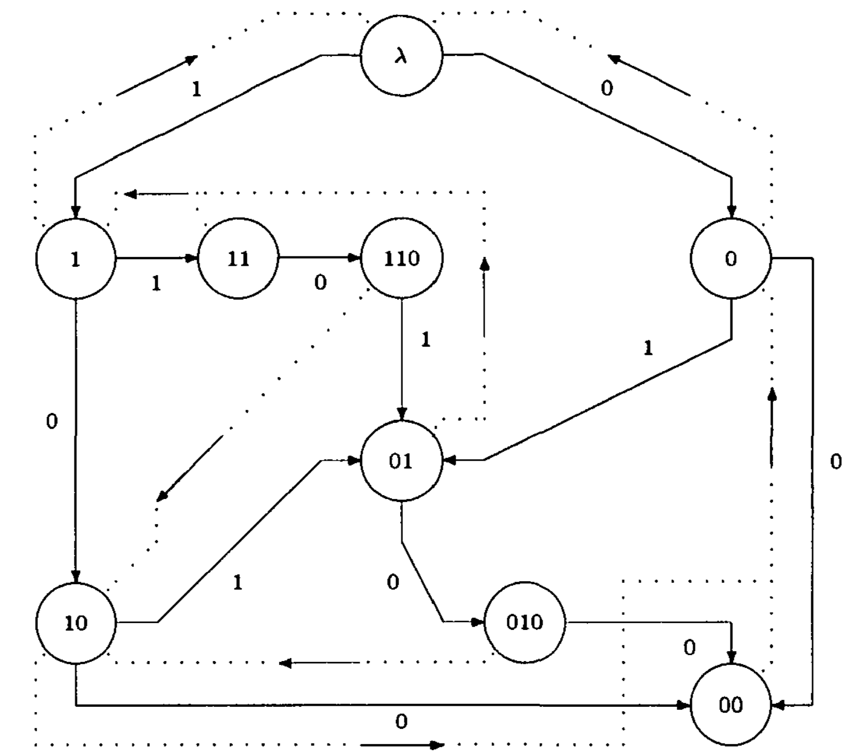
In [37] Jansen associated with the maximum depth of a direct acyclic word graph (DAWG) from . Below we recall a toy example in [37] to generate a DAWG from a binary string, which helps readers better understand relevant notions.
Example 1.
The sequence has the following set of all subsequences
where represents the empty sequence. For the sequence , the endpoints are given as
| 1 | 1 | 0 | 1 | 0 | 0 | ||
|---|---|---|---|---|---|---|---|
| endpoints | 0 | 1 | 2 | 3 | 4 | 5 | 6 |
For the sub-sequences of , their endpoints are given as below
Subsequences are considered equivalent if they have the same set of endpoints. For instance, the following are three equivalent classes with endpoints , and , respectively:
Therefore, the total 17 subsequences in are divided into equivalence classes. It’s customary to choose the shortest subsequence as the class representative. In this way, we have the following representatives:
From the above discussion, we can build a DAWG as follows: each representative in is denoted by a node and is considered as the source node; there is a directed edge between one node to another node iff the equivalence class of contains a subsequence, which extended with the edge symbol belongs to the equivalence class of ; the edges are divided into primary and secondary edges: an edge is primary iff it belongs to a primary path (the longest path from the source to the node) and a depth of a node is the length of the primary path to the node, where the length of a path is the number of edges along the path. Let be a subset consisting of nodes with more than one outgoing primary edges in and define the maximum depth .
In this way we obtain the DAWG of the sequence as in Figure 3, where primary edges are displayed in solid arrows. From the definition of the depth of a node, we have
Since , we have
With the notions illustrated in Example 1, Jansen in [14] established the following connection between the maximum-order complexity of a sequence and the depth of ADWG derived from , and proposed to calculate the maximum-order complexity of from its ADWG.
Proposition 7.
Given a sequence , the maximum-order complexity of and the depth of its ADWG satisfy
Blumer’s algorithm [39] were identified as an important tool to build an ADWG of a sequence , thereby calculating its maximum-order complexity profile in linear time and memory with regard to the sequence length. The method worked particularly well for periodic sequences. With this algorithm, Jansen exhausted all binary -length sequences and -periodic sequences as ranges from up to [14, Tables 3.1-3.4], which exhibited typical statistical behaviors of maximum-order complexity profiles of random sequences: the expected maximum-order complexity of a random sequence of sufficiently large length over is given by
Following the successful approach in [36], Rizomiliotis and Kalouptsidis [40] considered the calculation of the maximum-order complexity of a sequence in a similar way. From the recursive equations for , one can obtain a similar system to linear equations
where the coefficient matrix from all binary terms , where is any element in in a special ordering according to the degree of the terms. For instance, when and , the system of linear equations is given by
with
In [40] the authors investigated the properties of the -tuples as runs through the indices and proposed a term-by-term algorithm to compute the maximum-order complexity and output a feedback function for a given sequence . They also pointed out that the dominant multiplication complexity in their proposed algorithm is in the order of .
The above approach by analyzing the structure of is not satisfactory enough. Later in [41] the authors made more observations that further improved the performance of calculating maximum-order complexity of sequences.
Proposition 8.
For a binary sequence , suppose and the minimal FSR of does not generate . Then if and only if the subsequence has not appeared within .
The above observation is a natural extension of the property of maximum-order complexity in Lemma 1 (i). Instead, the following observation characterized the jump of maximum-order complexity profile at each term.
Proposition 9.
For a binary sequence , suppose . Let be the least integer such that for certain . Then Moreover, if for , then the sequence by arbitrary extension has the same maximum-order complexity .
In addition, they observed that the maximum-order complexity profile of a sequence has a close connection to its eigenvalue profile. To be more concrete, the eigenwords in a sequence are those subsequences of that are not contained in any proper subsequence of . They showed the following interesting connection.
Theorem 6.
For a binary sequence , suppose and the minimal FSR of does not generate . Then
where is the number of eigenwords in the sequence .
From the observations on the update of certain feedback function when the minimal FSR of does not generate , they proposed the following procedure to generate a minimal feedback function and maximum-order complexity of a sequence . Suppose and the minimal feedback function of is . Then
-
•
if , then and share the minimal feedback function and the same maximum-order complexity
-
•
if and , then update as
-
•
if and , then
Consequently, they proposed an efficient algorithm for maximum-order complexity, which works very similarly to the Berlekamp-Massey algorithm. For ease of comparison with the Berlekamp-Massey algorithm, we recall it in Algorithm 1. The computational complexity of Algorithm 1 in the worse case is , while in the average case is since the the expected maximum-order complexity . While it has the similar complexity as the ADWG method [14], its recursive nature is an important advantage since it eliminates the need to know the entire sequence in advance. This resembles the well-known Berlekamp-Massey algorithm in the linear case: if a discrepancy occurs at certain step, then a well-determined corrective function is added to the current minimal feedback function of to provide an updated minimal feedback of . In addition, the update of maximum-order complexity at each step is similar to for linear complexity of the sequence in the recursive procedure.
5.2 Approximate statistical behavior
Conducting a rigorous theoretical analysis of the behavior of maximum-order complexity profiles, as done for linear complexity, appeared intractable. On the other hand, maximum-order complexity had a lot of similarities as linear complexity. In order to facilitate the randomness test with maximum-order complexity, Erdman and Murphy proposed a method to approximate the distribution of the maximum-order complexity [42]. Inspired by the property of maximum-order complexity in Lemmas 1 and 2, they investigated a function that approximates the function : the probability that the first -tuples are all different in a sequence.
Proposition 10.
Let be the probability that the -th -tuple is unique given that the previous -tuples were unique. Then
Simulations on random sequences for from to [42, Table 2] indicated that the above approximation was accurate, particularly when .
Recall that a purely periodic sequence has maximum-order complexity if the first -tuples are unique but at least one of the first -tuples is repeated. Thus, for calculating a periodic sequence , it suffices to only look at the first bits to see if the -tuples are unique and the first bits to see if the -tuples are not unique. Denote by the probability that the first -tuples are unique while the -tuples are not. This probability function can be well approximated by , which is given by
Based on this approximation (of which the accuracy was shown in [42, Table 3]), the expected maximum-order complexity was approximated as follows:
Theorem 7.
Let be the maximum-order complexity of a random periodic binary sequence . Then
Similarly, for random binary sequences of length , the expected maximum-order complexity was approximated below.
Theorem 8.
Let be the number of binary sequences of length with maximum-order complexity . Then it can be approximated as
and the expected maximum-order complexity of random binary sequence of length is given by
5.3 Sequences with high maximum-order complexity
Different complexity measures were proposed in the literature to evaluate the randomness of sequences. Sequences with low complexity, including the linear, quadratic and maximum-order complexity, allow for short FSRs to generate the whole period of the sequences. This reveals that terms in those sequences are calculable when feedback functions generating them are determined. It is clear that such sequences should be avoided for any cryptographic applications. On the other hand, the relation between high complexity of a sequence and good randomness of a sequence is not well understood yet neither. For the aforementioned complexity measures, the sequences of the form have the largest complexity, but have clearly poor randomness. According to the exhaustive search results on maximum-order complexity in Tables 1-3 in [14], while sequences are the only instances of -length sequences that have the highest possible complexity , there are multiple -periodic binary sequences having the highest maximum-order complexity .
Researchers have been interested in the study of sequences with high maximum-order complexity [43, 44], particularly on sequences having highest possible maximum-order complexity [45, 46]. For the latter case, Rizomiliotis [40] in 2005 proposed the following necessary and sufficient condition for an -periodic binary sequence to have maximum-order complexity the same as its linear complexity.
Proposition 11.
For a periodic binary sequence , let be the polynomial representation of , and let , and . Then
| (9) |
iff there exists integers satisfying
when .
Based on the above condition, different families of -periodic binary sequences that have the same linear complexity and maximum-order complexity were proposed in [40]. Moreover, an algorithm based on Lagrange interpolation and an algorithm based on the relative shift of the component sequences were proposed to generate binary sequences with highest possible maximum-order complexity. These two ideas were further developed for constructing such periodic sequences with period of the form [45]. Roughly 10 years later, -periodic sequences with highest maximum-order complexity were revisited in [46], which provided a complete picture of all such sequences. The authors of [46] gave the necessary and sufficient condition for -periodic sequences over any alphabet to have maximum-order complexity .
Theorem 9.
Let be an -periodic sequence over any field . Then iff there exists an integer with such that for and for . Furthermore, such a sequence can, up to shift equivalence, be represented as one of the following forms
(1) where ;
(2) for certain integer with
and
where the integers for are derived from with ,
With the full characterization in Theorem 9, the distribution of random -periodic binary sequences having maximum-order complexity can be derived as follows.
Proposition 12.
The probability that a randomly generated sequence having highest is given by
where is the Euler’s totient function and is the Möbius function given by . In particular, when , the probability
Interestingly, the sequences characterized in Theorem 9 exhibit a strong recursive structure, which can be derived by applying the Euclidean algorithm on and the integer , a smaller period of a subsequence of . This strong recursive structure, on the other hand, implies that is far from being random. As discussed in [46], the balancedness, stability and scalability of such sequences are not good, indicating that they should be avoided for cryptographic applications. Very recently, binary sequences with periodic were further studied in [47], where the authors further investigated the structure of and proposed an algorithmic method to determine all -periodic binary sequences with maximum-order complexity .
In addition, Liang et al. recently investigated the structure of -length binary sequences with high maximum-order complexity and proposed an algorithm that can completely generate all those binary sequences [44]. Based on the completeness, they managed to provide an explicit expression of the number of -length binary sequences with any maximum-order complexity between and .
Proposition 13.
The number of -length binary sequences with maximum-order complexity with is given by
where
when is factorized as .
6 Relation between Complexity Measures
Besides the complexity measures in the context of FSRs in previous sections, some other measures have been discussed by researchers, such as Lempel-Ziv complexity [48], -adic complexity for FSRs with carry operation [15], -error complexity, expansion complexity [49], and correlation measure [50, 51]. This section will briefly review the relations among these measures. Below we start with the relation between the complexity measures in the previous sections, and we will be mainly focusing on extreme cases.
6.1 Relations between FSR-based complexities
From their definitions, for a sequence , it is easily seen that
We know that the special sequence of the form , where , has the largest linear complexity , quadratic and maximum-order complexity . As for -periodic sequences over , the largest linear complexity is also , which can be seen from the expression , as recalled in Proposition 5. This can be used to characterize the periodic sequences with largest linear complexity. Assume with , where is the characteristic of . Let be the cyclotomic cosets modulo relative to the power . Let be a primitive -th root of unity in an extension of . Then we have the following factorization of over :
which indicates that an -periodic sequences over has the largest linear complexity iff
Niederreiter in [52] proved the existence of -periodic sequences with the largest linear complexity and large -error linear complexity, which is defined as
This result was obtained by finding integers satisfying a condition, which was derived from the following observation [52]: let and suppose is an integer such that , then there exists an -periodic sequence satisfies
As shown in the examples in [52], there are infinitely many primes allowing for the existence of binary -periodic sequences of maximum possible linear complexity .
Finding -periodic sequences with the largest maximum-order complexity seems more challenging, especially when -error complexity is also considered. As recalled in Section 5, Sun et at. [46] revealed -periodic sequences with the largest maximum-order complexity , which have surprisingly strong recursive structure. Besides this, little result about -error maximum-order complexity and quadratic complexity has been reported. Here we propose two open problems for interested readers.
Problem 2.
Characterize/Determine all the -periodic sequences over with the largest quadratic complexity .
Problem 3.
Characterize certain lower bound on the -error maximum-order complexity of -periodic sequences with maximum-order complexity .
Another extreme case for sequences is that they have the least possible complexity values. For finite-length sequences, we know that the linear, quadratic and maximum-order complexity can be as small as zero, which don’t appear interesting to explore. When is a periodic sequence over , we know that m-sequences of length have the least complexities and DeBruijn sequences of length have the least maximum-order complexity In addition to the aforementioned observations, readers may wonder what else we know about their relations so far?
Due to the limited understanding of DeBruijn sequences, there have been only partial results for the above problem. It was well known [53] that the linear complexity of binary DeBruijn sequences of order is between and , where both the lower and upper bound are attainable. However, there exists no binary DeBruijn sequences with linear complexity [54]. Based on evidences on existing results, Etzion in his survey made the following conjecture:
Conjecture 3.
For any integer , there exists a binary DeBruijn sequence with minimal polynomial .
There is a close connection between m-sequence over of order and DeBruijn sequences of order . There have been also some works on the linear complexity of modified DeBruijn sequences, which obtained by removing one zero from the longest run of zeros in a DeBruijn sequence. Mayhew and Golomb [55] showed that the minimal polynomial of binary modified DeBruijn sequences of order is a product of distinct irreducible polynomials with degrees not equal to and dividing . Further results on the restrictions of the degrees were developed in [56, 57, 58].
When considering the fact for a binary sequence with low quadratic complexity , any subsequence of length slightly larger than can be sufficient to recover the whole sequence . However, the topic of quadratic complexity was significantly less explored. There has been little research progress on the quadratic complexity although it was already studied in 1989. To the best of my knowledge, only result about the quadratic complexity of DeBruijn sequences were report by Chan and Games [16].
Proposition 14.
Given a binary DeBruijn sequence of order , then
In particular, this upper bound can be attained by the DeBruijn sequence derived from an m-sequence of order by including the all zero -tuple.
6.2 FSR-based complexities, Lempel-Ziv complexity, expansion complexity, and autocorrelation
This subsection will briefly review recent works on the relations among the linear, maximum-order complexity and other significant metrics for assessing pseudo-random sequences.
6.2.1 2-adic complexity
The 2-adic complexity introduced by Goresky and Klapper [60, 15] is closely related to the length of a shortest feedback with carry shift register (FCSR) that generates the sequence. The theory of 2-adic complexity of periodic sequences has been well developed. Given a sequence , one has
where and
The -adic complexity of is defined as . In the aperiodic case, the -th 2-adic complexity, denoted by , is the binary logarithm of
There was very little work on exploring the relation between linear, quadratic and maximum-order complexities of a binary sequence and its -adic complexity. Until recently it was shown [61] that the maximum-order complexity of a binary sequence is upper bounded by its 2-adic complexity.
6.2.2 Lempel-Ziv complexity
The Lempel-Ziv complexity of a sequence is one classical complexity measure based on pattern counting, introduced by Lempel and Ziv in 1976 [48] and later named after them. The parsing procedure in the calculation of Lempel-Ziv complexity laid the basis for the prominent Lempel-Ziv compression algorithms [62, 63]. The Lempel-Ziv complexity reflects the compressibility of a sequence and thus has significant cryptographic interest.
The Lempel-Ziv complexity measures the rate at which new patterns emerge as we move along a given sequence. For a binary sequence , we split up into adjacent blocks. By definition, the first block consists of . If is a union of blocks, or in other words if is the last bit in a block, then the next block is uniquely determined by two properties: i) the sequence occurs as a subsequence in ; ii) the sequence does not occur as a subsequence in . The Lempel-Ziv complexity is then the number of blocks into which is split up by this procedure.
Motivated by Niederreiter’s statement [22], Limniotis, Kolokotronis and Kalouptsidis explored the relation between the maximum-order complexity and Lempel-Ziv complexity of a sequence, which are both closely connected to the eigenvalue profile of the sequence. They pointed out that although the exhaustive history (which uniquely determines the Lempel-Ziv complexity) cannot fully estimate the maximum-order complexity profile and vise versa, there still exists a relationship between them in the sense that the eigenvalue profile of a sequence of given Lempel-Ziv complexity, which determines the maximum-order complexity profile, is restricted rather than arbitrary. They also established a lower bound on the compression ratio of sequences with a prescribed maximum-order complexity.
6.2.3 Expansion complexity
In 2012, Diem introduced the notion of expansion complexity of sequences [17], in which he showed that the sequences over finite fields with optimal linear complexity proposed by Xing and Lam via function expansion [19] can be efficiently computed from a relatively short subsequence.
Let be a sequence over . For a positive integer , the th expansion complexity is 0 if and otherwise the least total degree of a nonzero polynomial with
where the total degree of is given by
The expansion complexity of the sequence is defined as
It can be verified that . In particular, if is restricted to be irreducible, then the -th irreducible expansion complexity and irreducible expansion complexity of can be defined accordingly. The relations between the linear complexity, maximum-order complexity and expansion complexity were discussed recently in [49, 64].
Proposition 15.
Let be an ultimately periodic sequence with pre-period , period and linear complexity . Then the irreducible expansion complexity
and otherwise.
Proposition 16.
For any infinite sequence over , if with and , then its th expansion complexity is no more than .
6.2.4 -order correlation measure
Let be a positive integer. The -th correlation measure of order of a binary sequence is given by [65]
where the maximum is taken over all with non-negative integers and such that .
The relations between the linear complexity, maximum-order complexity and correlation measure of order were explored in [65, 50, 51].
Proposition 17.
Given a binary sequence , the -th linear complexity and -th correlation measure of satisfy
and the -th maximum-order complexity and -th correlation measure of satisfy
The above bounds was recently improved in [51].
Proposition 18.
Given a binary sequence , if for some integer , the -th linear complexity of satisfies
then for some with , one has
In addition, if the -th maximum-order complexity of satisfies , then one has
7 Conclusion
This survey primarily focused on the complexity measures of sequences within the domain of feedback shift registers, which are efficiently computable and hold significant interest in cryptographic applications. Notable works on the computation, stochastic behavior, and theoretic result on these complexities were examined to a certain technical extent. Several conjectures were revisited and new open problems were proposed. To offer a sounding overview of the research development on complexity measures, we also briefly reviewed the established relation between these complexities as well as their connection with other important metrics for pseudo-random sequences, including the well-known 2-adic complexity, Lempel-Ziv complexity, expansion complexity and -order correlation measure. The survey indicates that although the study of complexity measures of randomness traces back to the 1960s, only linear complexity and maximum-order complexity could be considered relatively well explored. Other complexity measures and their interrelations appear more intractable and require new tools, techniques and theoretic studies in future researches.
References
- [1] R. V. Mises, “Grundlagen der Wahrscheinlichkeitsrechnung,” Mathematische Zeitschrift, vol. 5, no. 1, pp. 52–99, Mar. 1919.
- [2] A. Church, “On the concept of a random sequence,” Bulletin of the American Mathematical Society, vol. 46, no. 2, pp. 130–135, Feb. 1940.
- [3] S. W. Golomb, Shift Register Sequences: Secure and Limited-access Code Generators, Efficiency Code Generators, Prescribed Property Generators, Mathematical Models (third Revised Edition). World Scientific Publishing Company, 2017.
- [4] P. Martin-Löf, “The definition of random sequences,” Inforomation and Control, vol. 9, no. 6, pp. 602–619, Dec. 1966.
- [5] A. N. Kolmogorov, “Three approaches to the quantitative definition of information*,” International Journal of Computer Mathematics, vol. 2, no. 1–4, pp. 157–168, Jan. 1968.
- [6] C. Schnorr, “Process complexity and effective random tests,” Journal of Computer and System Sciences, vol. 7, no. 4, pp. 376–388, Aug. 1973.
- [7] D. E. Knuth, The Art of Computer Programming, Volume 2: Seminumerical Algorithms, 3rd ed. Boston: Addison-Wesley, 1997.
- [8] E. R. Berlekamp, Algebraic Coding Theory. Singapore: World Scientific Publishing Company, Oct. 1968.
- [9] J. Massey, “Shift-register synthesis and BCH decoding,” IEEE Transactions on Information Theory, vol. 15, no. 1, pp. 122–127, Jan. 1969.
- [10] R. A. Rueppel, “Linear complexity and random sequences,” in Advances in Cryptology — EUROCRYPT’ 85, F. Pichler, Ed. Berlin, Heidelberg: Springer Berlin Heidelberg, 1986, pp. 167–188.
- [11] H. Niederreiter, “The probabilistic theory of linear complexity,” in Advances in Cryptology — EUROCRYPT ’88, ser. Lecture Notes in Computer Science. Springer Berlin Heidelberg, 1988, Book Section, pp. 191–209.
- [12] ——, “Linear complexity and related complexity measures for sequences,” in Progress in Cryptology - INDOCRYPT 2003, ser. Lecture Notes in Computer Science. Springer, 2003, Book Section, pp. 1–17.
- [13] L. E. Bassham, A. L. Rukhin, J. Soto, J. R. Nechvatal, M. E. Smid, S. D. Leigh, M. Levenson, M. Vangel, N. A. Heckert, and D. L. Banks, “A statistical test suite for random and pseudorandom number generators for cryptographic applications,” NIST, Sep. 2010.
- [14] C. J. A. Jansen, “Investigations on nonlinear streamcipher systems: construction and evaluation methods,” phdthesis, Delft University of Technology, 1989.
- [15] A. Klapper and M. Goresky, “Feedback shift registers, 2-adic span, and combiners with memory,” Journal of Cryptology, vol. 10, no. 2, pp. 111–147, Mar. 1997.
- [16] A. H. Chan and R. A. Games, “On the quadratic spans of DeBruijn sequences,” IEEE Transactions on Information Theory, vol. 36, no. 4, pp. 822–829, 1990.
- [17] C. Diem, “On the use of expansion series for stream ciphers,” LMS Journal of Computation and Mathematics, vol. 15, pp. 326–340, Sep. 2012.
- [18] A. Topuzoğlus and A. Winterhof, “Pseudorandom sequences,” in Topics in Geometry, Coding Theory and Cryptography, A. Garcia and H. Stichtenoth, Eds. Springer, 2006, pp. 135–166.
- [19] C. Xing and K. Y. Lam, “Sequences with almost perfect linear complexity profiles and curves over finite fields,” IEEE Transactions on Information Theory, vol. 45, no. 4, pp. 1267–1270, May 1999.
- [20] C. Xing, K. Y. Lam, and Z. Wei, “A Class of Explicit Perfect Multi-sequences,” in Advances in Cryptology - ASIACRYPT’99. Berlin, Germany: Springer, 1999, pp. 299–305.
- [21] H. Niederreiter and M. Vielhaber, “An algorithm for shifted continued fraction expansions in parallel linear time,” Theoretical Computer Science, vol. 226, no. 1, pp. 93–104, Sep. 1999.
- [22] H. Niederreiter, “Some computable complexity measures for binary sequences,” in Sequences and their Applications. Springer London, 1999, pp. 67–78.
- [23] D. Jungnickel, Finite fields: Structure and arithmetics. B.I. Wissenschaftsverlag, Jan. 1993.
- [24] J. L. Massey and S. Serconek, “Linear complexity of periodic sequences: A general theory,” in Advances in Cryptology — CRYPTO ’96, N. Koblitz, Ed. Berlin, Heidelberg: Springer Berlin Heidelberg, 1996, pp. 358–371.
- [25] ——, “A Fourier Transform Approach to the Linear Complexity of Nonlinearly Filtered Sequences,” in Advances in Cryptology - CRYPTO’94. Berlin, Germany: Springer, Jul. 1994, pp. 332–340.
- [26] R. E. Blahut, Theory and Practice of Error Control Codes. Addison-Wesley Publishing Company, 1983.
- [27] E. S. Selmer, Linear Recurrence Relations Over Finite Fields. Department of Informatics, University of Bergen, 1966.
- [28] C. Ding, T. Hesseseth, and W. Shan, “On the linear complexity of Legendre sequences,” IEEE Transactions on Information Theory, vol. 44, no. 3, pp. 1276–1278, May 1998.
- [29] W. Meidl and A. Winterhof, “Lower bounds on the linear complexity of the discrete logarithm in finite fields,” IEEE Transactions on Information Theory, vol. 47, no. 7, pp. 2807–2811, Nov. 2001.
- [30] T. Helleseth, S.-H. Kim, and J.-S. No, “Linear complexity over and trace representation of Lempel-Cohn-Eastman sequences,” in Proceedings IEEE International Symposium on Information Theory. IEEE, 2003.
- [31] I. Shparlinski, Cryptographic Applications of Analytic Number Theory. Basel, Switzerland: Birkhäuser, 2003.
- [32] R. A. Rueppel, Analysis and Design of Stream Ciphers. Springer Berlin Heidelberg, 1986.
- [33] W. Meidl and H. Niederreiter, “On the expected value of the linear complexity and the -error linear complexity of periodic sequences,” IEEE Transactions on Information Theory, vol. 48, no. 11, pp. 2817–2825, 2002.
- [34] A. H. Chan and R. A. Games, “On the quadratic spans of periodic sequences,” in Advances in Cryptology — CRYPTO’ 89 Proceedings, ser. Lecture Notes in Computer Science. Springer, 1990, Book Section, pp. 82–89.
- [35] A. Youssef and G. Gong, “On the quadratic span of binary sequences,” in Proceeding of the 20th Biennial Symposium on Communications, Queen’s university, 2000, pp. 159–163.
- [36] P. Rizomiliotis, N. Kolokotronis, and N. Kalouptsidis, “On the quadratic span of binary sequences,” IEEE Transactions on Information Theory, vol. 51, no. 5, pp. 1840–1848, Apr. 2005.
- [37] C. Jansen and D. Boekee, “The shortest feedback shift register that can generate a given sequence,” in Advances in Cryptology – CRYPTO’89 Proceedings, ser. Lecture Notes in Computer Science. Springer, 1990, Book Section, pp. 90–99.
- [38] C. Jansen, “The maximum order complexity of sequence ensembles,” in Advances in Cryptology — EUROCRYPT ’91, ser. Lecture Notes in Computer Science. Springer, 1991, Book Section, pp. 153–159.
- [39] A. Blumer, J. Blumer, A. Ehrenfeucht, D. Haussler, and R. M. McConnell, “Linear size finite automata for the set of all subwords of a word - an outline of results,” Bulletin of the EATCS, vol. 21, pp. 12–20, 1983.
- [40] P. Rizomiliotis and N. Kalouptsidis, “Results on the nonlinear span of binary sequences,” IEEE Transactions on Information Theory, vol. 51, no. 4, pp. 1555–1563, Apr. 2005.
- [41] K. Limniotis, N. Kolokotronis, and N. Kalouptsidis, “On the nonlinear complexity and Lempel–Ziv complexity of finite length sequences,” IEEE Transactions on Information Theory, vol. 53, no. 11, pp. 4293–4302, 2007.
- [42] D. Erdmann and S. Murphy, “An approximate distribution for the maximum order complexity,” Designs, Codes and Cryptography, vol. 10, no. 3, pp. 325–339, Mar. 1997.
- [43] Y. Luo, C. Xing, and L. You, “Construction of Sequences With High Nonlinear Complexity From Function Fields,” IEEE Transactions on Information Theory, vol. 63, no. 12, pp. 7646–7650, Aug. 2017.
- [44] S. Liang, X. Zeng, Z. Xiao, and Z. Sun, “Binary sequences with length n and nonlinear complexity not less than ,” IEEE Transactions on Information Theory, vol. 69, no. 12, pp. 8116–8125, Sep. 2023.
- [45] P. Rizomiliotis, “Constructing periodic binary sequences with maximum nonlinear span,” IEEE Transactions on Information Theory, vol. 52, no. 9, pp. 4257–4261, Aug. 2006.
- [46] Z. Sun, X. Zeng, C. Li, and T. Helleseth, “Investigations on Periodic Sequences With Maximum Nonlinear Complexity,” IEEE Transactions on Information Theory, vol. 63, no. 10, pp. 6188–6198, Jun. 2017.
- [47] Q. Yuan, C. Li, X. Zeng, T. Helleseth, and D. He, “Further investigations on nonlinear complexity of periodic binary sequences,” IEEE Transactions on Information Theory, pp. 1–1, 2024.
- [48] A. Lempel and J. Ziv, “On the Complexity of Finite Sequences,” IEEE Transactions on Information Theory, vol. 22, no. 1, pp. 75–81, Jan. 1976.
- [49] L. Merai, H. Niederreiter, and A. Winterhof, “Expansion complexity and linear complexity of sequences over finite fields,” Cryptography and Communications-Discrete-Structures Boolean Functions and Sequences, vol. 9, no. 4, pp. 501–509, 2017. [Online]. Available: ¡Go to ISI¿://WOS:000410834000005 https://link.springer.com/content/pdf/10.1007/s12095-016-0189-2.pdf
- [50] L. Işık and A. Winterhof, “Maximum-order complexity and correlation measures,” Cryptography, vol. 1, no. 1, p. 7, May 2017.
- [51] Z. Chen, A. I. Gómez, D. Gómez-Pérez, and A. Tirkel, “Correlation measure, linear complexity and maximum order complexity for families of binary sequences,” Finite Fields and Their Applications, vol. 78, p. 101977, Feb. 2022.
- [52] H. Niederreiter, “Periodic sequences with large -error linear complexity,” IEEE Transactions on Information Theory, vol. 49, no. 2, pp. 501–505, Feb. 2003.
- [53] A. H. Chan, R. A. Games, and E. L. Key, “On the complexities of de bruijn sequences,” Journal of Combinatorial Theory, Series A, vol. 33, no. 3, pp. 233–246, Nov. 1982.
- [54] R. A. Games, “There are no DeBruijn sequences of span with complexity ,” Journal of Combinatorial Theory, Series A, vol. 34, no. 2, pp. 248–251, Mar. 1983.
- [55] G. Mayhew and S. Golomb, “Linear spans of modified bruijn sequences,” IEEE Transactions on Information Theory, vol. 36, no. 5, pp. 1166–1167, 1990.
- [56] G. M. Kyureghyan, “Minimal polynomials of the modified DeBruijn sequences,” Discrete Applied Mathematics, vol. 156, no. 9, pp. 1549–1553, May 2008.
- [57] Y.-J. Dong, T. Tian, W.-F. Qi, and Z.-X. Wang, “New results on the minimal polynomials of modified de bruijn sequences,” Finite Fields and Their Applications, vol. 60, p. 101583, Nov. 2019.
- [58] H.-Y. Wang, Q.-X. Zheng, Z.-X. Wang, and W.-F. Qi, “The minimal polynomials of modified DeBruijn sequences revisited,” Finite Fields and Their Applications, vol. 68, p. 101735, Dec. 2020.
- [59] L. H. Khachatrian, “The lower bound of the quadratic spans of DeBruijn sequences,” Designs, Codes and Cryptography, vol. 3, no. 1, pp. 29–32, Mar. 1993.
- [60] A. Klapper and M. Goresky, “Cryptanalysis based on 2-adic rational approximation,” in Advances in Cryptology — CRYPTO’ 95. Springer Berlin Heidelberg, 1995, pp. 262–273.
- [61] Z. Chen, Z. Chen, J. Obrovsky, and A. Winterhof, “Maximum-order complexity and -adic complexity,” arXiv, 2023.
- [62] J. Ziv and A. Lempel, “A universal algorithm for sequential data compression,” IEEE Transactions on Information Theory, vol. 23, no. 3, pp. 337–343, May 1977.
- [63] ——, “Compression of individual sequences via variable-rate coding,” IEEE Transactions on Information Theory, vol. 24, no. 5, pp. 530–536, Sep. 1978.
- [64] Z. Sun, X. Zeng, C. Li, Y. Zhang, and L. Yi, “The expansion complexity of ultimately periodic sequences over finite fields,” IEEE Transactions on Information Theory, vol. 67, no. 11, pp. 7550–7560, Nov. 2021.
- [65] N. Brandstätter and A. Winterhof, “Linear complexity profile of binary sequences with small correlation measure,” Periodica Mathematica Hungarica, vol. 52, no. 2, pp. 1–8, Jun. 2006.