Impurity Parallel Velocity Gradient instability
Abstract
In magnetized plasmas, a radial gradient of parallel velocity, where parallel refers to the direction of magnetic field, can destabilise an electrostatic mode called as Parallel Velocity Gradient (PVG). The theory of PVG has been mainly developed assuming a single species of ions. Here, the role of impurities is investigated based on a linear, local analysis, in a homogeneous, constant magnetic field. To further simplify the analysis, the plasma is assumed to contain only two ion species - main ions and one impurity species - while our methodology can be straightforwardly extended to more species. In the cold-ion limit, retaining polarization drift for both main ions and impurity ions, and assuming Boltzmanian electrons, the system is described by 4 fluid equations closed by quasineutrality. The linearized equations can be reduced to 2 coupled equations: one for the electric potential, and one for the effective parallel velocity fluctuations, which is a linear combination of main ion and impurity parallel velocity fluctuations. This reduced system can be understood as a generalisation of the Hasegawa-Mima model. With finite radial gradient of impurity parallel flow, the linear dispersion relation then describes a new instability: the impurity PVG (i-PVG). Instability condition is described in terms of either the main ion flow shear, or equivalently, an effective flow shear, which combines main ion and impurity flow shears. Impurities can have a stabilising or destabilising role, depending on the parameters, and in particular the direction of main flow shear against impurity flow shear. Assuming a reasonable value of perpendicular wavenumber, the maximum growthrate is estimated, depending on impurity mass, charge, and concentration.
1 Introduction
In magnetized plasmas, the Parallel Velocity Gradient (PVG), or Parallel Velocity Shear (PVS) is a type of Kelvin-Helmholtz fluid instability driven by a radial gradient of parallel (to magnetic field) plasma flow. It is sometimes referred to as D’Angelo instability, since D’Angelo investigated a simplified version (simplified by a radial WKB approximation) for a low-temperature plasma in a uniform magnetic field [1]. The D’Angelo instability was then observed in basic plasma experiments [2, 3].
In toroidal magnetic confinement fusion devices, magnetic shear is stabilising [4]. However, theory indicates that PVG-driven turbulence may be found in the vicinity of transport barriers [5, 6], in the SOL [7], in the presence of strong parallel beam injection, and more readily in spherical tokamaks [8, 9]. Even in cases where PVGs are weak, they can have important impact by coupling with Ion-Temperature-Gradient (ITG) turbulence. Theory predicted subcritical ITG-PVG turbulence [10, 11, 12, 13], which is consistent with measurements (by Beam Emission Spectroscopy) on MAST [14]. Strong experimental hints, from fluctuation level and isotropy of correlation length, indicate a significant contribution of PVG-driven turbulence in the edge of the CT-6B tokamak plasma [15]. The universality of PVGs in tokamaks remains an open issue.
Parallel flows are also expected to play major roles in linear magnetized plasma devices, such as PANTA (Plasma Assembly for Nonlinear Turbulence Analysis, formerly LMD), where an uphill, near-axis, axial particle flux [16] has been measured to be consistent with PVG/drift-waves coupling [17], with a regime transition in quantitative agreement with the theoretical linear instability threshold [18].
Magnetic confinement fusion plasmas are often contaminated by ion species other than hydrogen isotopes, which are then called as impurities. These can include helium, nitrogen, neon, argon, beryllium, carbon, and tungsten.
Linear magnetized plasma experiments can also include impurities. In particular, a new linear device, called SPEKTRE (Sheath, Plasma Edge Kinetic Turbulence Radiofrequency Experiment) [19] and currently under construction, is partly designed to inject various impurities in a controlled manner and investigate their impact and their dynamics.
Our objective here is to investigate the instability driven by a radial shear of the parallel flows of multiple species, which we refer to as impurity-PVG (i-PVG). We consider experimental conditions that are relevant to linear plasma experiments with cylindrical geometry such as PANTA and SPEKTRE, and are insightful approximations of tokamak’s edge plasma, where the PVG instability is of its most significance. Our local, linearized model can be understood as a modified Hasegawa-Mima model including equilibrium and perturbed parallel velocities of both main ions and impurities.
In the case of slab geometry with weak magnetic shear, Guo obtained from gyrokinetic equations a linear dispersion relation for PVG with impurities, showing the stabilization of the PVG instability by the presence of impurities and by the increase of electron density gradient [20]. Here we adopt a fluid approach, and investigate how the i-PVG threshold, frequency and growth-rate depend on parameters such as impurity charge, mass, concentration and parallel flow shear. We further assume a cold-ion limit to provide clearer analysis of the i-PVG. Our fluid approach is supported by this cold ion assumption, plus by the fact that our study focuses on the linear growth of the instabilities and ignores the damped states, so that kinetic effects such as Landau damping can be neglected. Compare to Guo’s previous work, our approach provides a more flexible analysis in terms of parameter scan for independent ion and impurity flow shears, and demonstrates that the presence of impurity can be either stabilizing or destabilizing for PVG. The relationship between linear properties and plasma parameters turns out to be somewhat complex, with several non-monotonous dependencies.
2 Model
The model is based on a local approximation in a Cartesian basis (, , ). The magnetic field is assumed homogeneous and constant, . Hereafter, the parallel and perpendicular subscripts ( and ) refer to the direction of the magnetic field and the perpendicular plane (, ). For each species , both equilibrium density gradient and equilibrium parallel velocity gradient are assumed constant and in the direction:
| (1) |
| (2) |
where and are the density gradient length and parallel velocity gradient length.
We assume for simplicity that the plasma contains only electrons () and two ion species (one main ion species , and one impurity species ), although the model can be straightforwardly generalized to more species. For each species, mass is noted , and charge is noted , where is the elementary charge ( and for simplicity we assume that the main ions satisfy ).
We adopt the cold ion limit, setting for the wave number an approximate maximum limit , with and , and being the Larmor radius of species . The perpendicular motion of ions (both main ions and impurity ions) is dominated by drift,
| (3) |
and polarization drift,
| (4) |
This is valid up to first order in terms of the ratio between wave frequency and cyclotron frequency, . Here, as verified a posteriori, remains as small as a few percents. However, since , the model requires heavy impurities to be sufficiently ionized (unless these impurities are in high enough concentration to bring down to small enough values).
These assumptions yield a system of four fluid equations. Namely, for each of and , the density equation writes as
| (5) |
and the parallel flow equation writes as
| (6) |
Assuming that electron density responds to electrostatic fluctuations according to a Boltzmann distribution, the system of equations is closed by quasi-neutrality,
| (7) |
where is the temperature.
3 Linear analysis
To obtain the linear dispersion relation, densities and parallel velocities are split into equilibrium and fluctuation parts, and . Then, Eqs. (5)-(7) are linearized,
| (8) |
| (9) |
| (10) |
Here we used the assumption of homogeneous magnetic field to remove the term in . In addition, we neglected four terms which remain small for typical plasma parameters:
-
1.
The term is of order compared to . Note that, compared to , it is of order , which, as verified a posteriori, remains much smaller than unity as long as .
-
2.
Similarly, the term is of order compared to .
-
3.
The term , compared to , is of order , which must remain small to avoid strong Landau damping. Note that, compared to , it is of order , where is the Mach number for species . To obtain the latter ordering, we substituted Eq. (20), and assumed that for each species, density and parallel gradient lengths are comparable. Extension of this theory for plasmas where the condition is not satisfied, is left for future work, as accounting for the term expands a parameter space that is already very large.
-
4.
Similarly, the term , compared to , is of order .
A linear combination reduces the system Eqs. (8)-(10) to two coupled equations, on the effective variables and , where is the equilibrium concentration of species . The two coupled equations write
| (11) |
| (12) |
where
| (13) |
is a linear combination of ion Larmor radii, is the electron diamagnetic drift velocity, is the ion-acoustic velocity including the contribution of impurities,
| (14) |
(recalling we adopt the cold ion limit), and, most importantly,
| (15) |
is a linear combination of main ion and impurity parallel velocity gradients, which we refer to as the effective flow shear. It is the source of free-energy of the i-PVG instability. Note that throughout this paper, we note the radial gradient () as (without a subscript). Let us define the ratio of parallel velocity gradients, . Then the effective flow shear can also be written as .
The above model can in fact be seen as a modification of the Hasegawa-Mima model, including the effective flow shear.
Fourier analysis yields the dispersion relation,
| (16) |
where
| (17) |
is the drift-wave frequency modified by impurities, and
| (18) |
is a linear combination of main ion and impurity cyclotron frequencies.
When the parallel wave number is , with
| (20) |
the function reaches its minimum value
| (21) |
Therefore, the linear instability condition can be written in terms of the effective flow shear, with
| (22) |
or, alternatively, in terms of the main ion flow shear, with
| (23) |
When an i-PVG wave is unstable, its frequency is and its growthrate is . These expressions are given in Eqs. (17) and (19). Note that the factor 2 in the frequency is mainly due to the finite value of – the i-PVG frequency does recover the impurity-modified drift-wave frequency in the limit of and .
For a given set of plasma parameters and a given value of , the maximum growthrate is reached for and , in which case
| (24) |
Hereafter we focus on that case , which is also more consistent with our local model.
4 Application to typical plasmas
For concision, let us note the mass ratio, and the ratio of parallel velocity gradients. Table 1 shows the parameters of a reference case, designed to be representative of a fusion plasma with highly ionized tungsten. The values and are consistent with measurements [21, 22]. Hereafter, we present analyses of cases which are variations of this reference case. The varying parameters are summarized in Table 2.
| Reference case | 10 | 0.1 | 2 | 184 | 40 | 0 | 0.7 |
| Fig. 1 | 0.1 | 2 | 12 and 184 | 6 and 40 | 0 and | 0.7 | -0.02 – 0.08 |
| Fig. 2 | 0.1 | 2 | 184 | 40 | -1 – 1 | -0.1 – 0.1 | |
| Fig. 3 | 0.1 | 2 | 12 and 184 | 6 and 40 | 0 and | 0 – 2 | |
| Fig. 4 | - | 2 | 0 – 200 | 0 – 200 | 0.7 | ||
| Fig. 5 | 0.1 | -1 – 2 | 5 – 200 | 5 | – | 0.7 | |
| Fig. 6 | 0.1 | -1 – 2 | 184 | 0 – 50 | – | 0.7 | |
| Fig. 7 | 0.1 | -1 – 2 | 12 – 184 | 3 – 40 | – | 0.7 | |
| Fig. 8 | 0.08 | 2 | 12 and 184 | 6 and 40 | 0 and | 0 – 2 | |
| Fig. 9 | 0.08 | 2 | 0 – 200 | 0 – 200 | 0.7 | ||
| Fig. 10 | 0.08 | -1 – 2 | 5 – 200 | 5 | – | 0.7 | |
| Fig. 11 | 0.08 | -1 – 2 | 184 | 0 – 50 | – | 0.7 | |
| Fig. 12 | 0.08 | -1 – 2 | 12 – 184 | 3 – 40 | – | 0.7 |
4.1 Dispersion relation
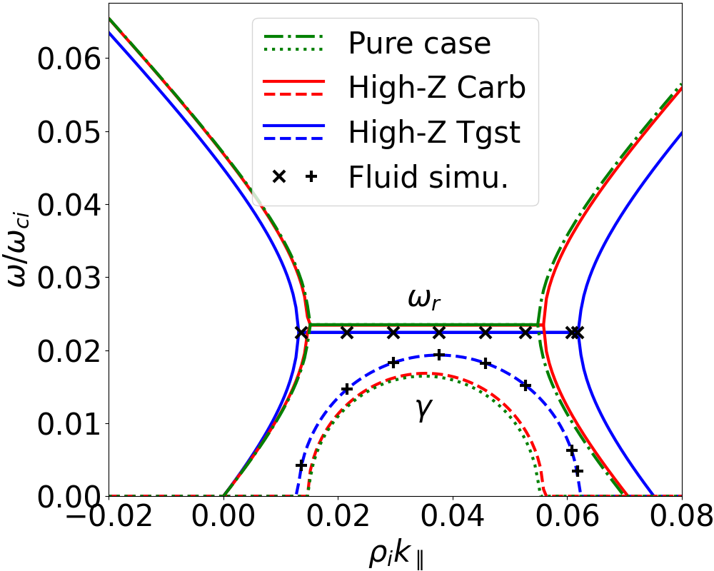
Figure 1 shows the dispersion relation for the reference case, as well as for C6+ ( and ) impurity. The dispersion relation of the pure PVG is included for comparison. We observe that the dispersion relation is qualitatively similar for the pure and impure cases, but quantitatively different. As demonstrated hereafter, differences are more important closer to the PVG instability threshold, or for higher impurity concentrations.
Let us now verify both the accuracy of the assumptions (i)–(iv) described in Sec. 3, and the correctness of our linear analysis. We developed an initial value numerical simulation code to solve the fluid model Eqs. (5-7), which does not rely on the assumptions (i)–(iv). Time integration is performed by an explicit RK4 scheme with time-step width . All quantities (, , ) are described in Fourier space (, ) on a 256x256 grid for a fixed . Nonlinear terms such as are computed in real space before being transformed back to Fourier space. Fig. 1 includes the frequency and growthrate extracted from time-traces of complex Fourier component of , during the linear phase. There is good quantitative agreement for the values of such that the growthrate is close to its maximum – the relative error for the growthrate remains below for the range . The relative error can be as high as a few percents in the range or a few tens of percent in the range , but these weak modes are negligible in the linear phase of the instability. The relative error for the frequency remains below for the whole unstable range.
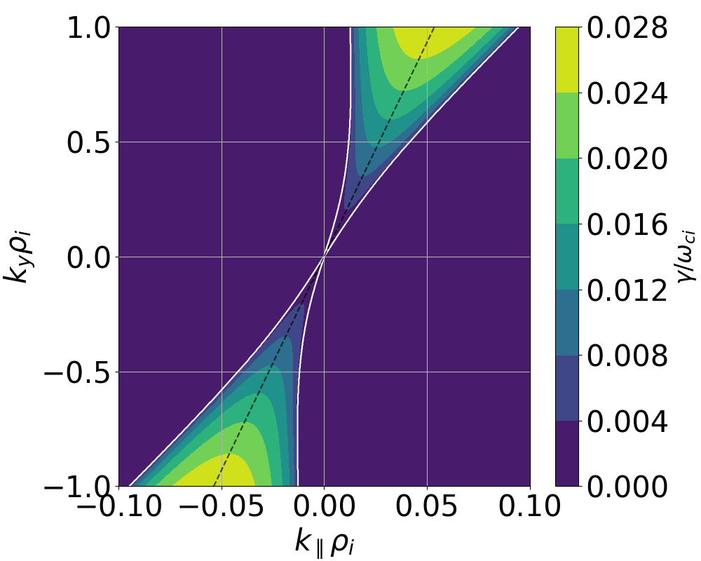
Figure 2 shows the linear growthrate in the space of wavevector components (, ). The asymmetry in this space, instability occurring only for (for ), is an important property of the i-PVG. If the sign of was flipped, the unstable region would be in the region . As expected, growthrate is maximum for . Hereafter, we always set .
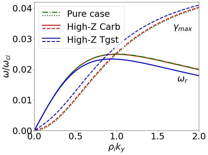
Figure 3 displays the maximum growthrate (obtained for ) against the azimuthal wavenumber, as well as the corresponding frequency. Our model does not include any mechanism for small scale dissipation. As a consequence, spuriously keeps on increasing for increasing . However, our model looses its validity as approches unity. With the knowledge of the typical shape of obtained from more complete models for many instabilities, let us, as a first, qualitative approach, approximate the physical maximum growthrate by choosing a cut-off at . Then, for our reference case, the maximum growthrate is .
In summary, the results in this section confirm that the linear properties of the i-PVG instability are qualitatively the same as that of the pure PVG instability. For the chosen set of parameters, even the quantitative differences are small. However, that is for a case where the pure PVG instability is already quite strong, since . In this sense, the above results concern a range far from instability threshold. By contrast, in the next section we focus on the instability threshold itself.
4.2 Critical ionic PVG
As explained in Sec. 3, for a given set of parameters (, , , , , ), and bounded value of , the i-PVG instability threshold can be expressed either in terms of the effective flow shear, which is a combination of main ion and impurity flow shears, or, alternatively, in terms of the main ion flow shear alone. The corresponding thresholds are given by Eqs. (22) and (23), respectively. The preferred point-of-view may depend on the experimental conditions which determine preferred control parameters. Here we focus on the second point-of-view, that of critical main ion flow shear for a given ratio .
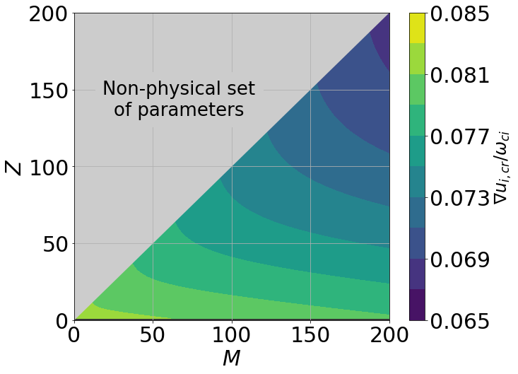
Figure 4 displays the critical main ion flow shear against mass and charge ratio, for and . It is clear that i-PVG-unstable conditions are more readily reached when the impurity is massive and highly ionized. In realistic machines however, radiation from high-mass and high-Z impurities is a severe issue, so that the applicability of such ranges of parameters should be carefully studied. On the contrary, at this low concentration, the threshold for low-mass, low-charge impurities is not so different than the threshold for high-mass, low-charge impurities, and is actually close to the threshold of the pure PVG.
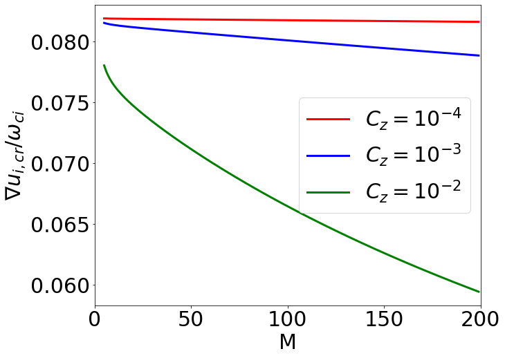
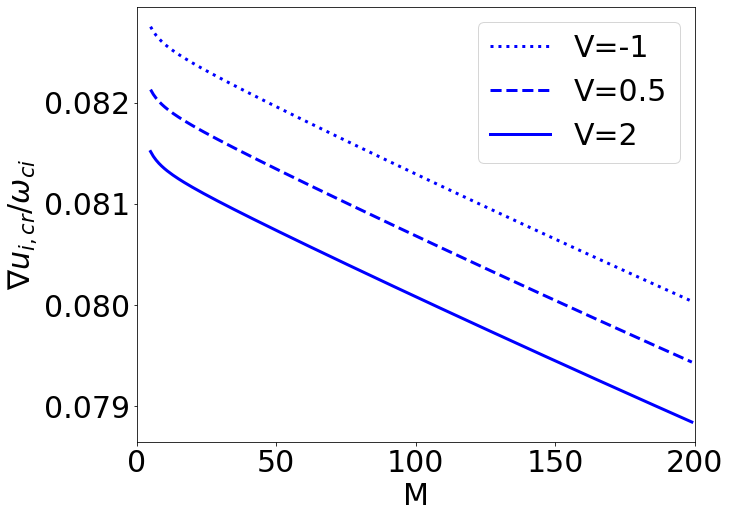
Figure 5 illustrates the role of the mass ratio, at fixed , for various impurity concentrations and various flow shear ratios . The critical main ion flow shear is always decreasing with increasing mass ratio, but the relationship is nonlinear. Here the impact of is small, but that is because and are both low, such that the i-PVG is actually very close to the pure PVG.
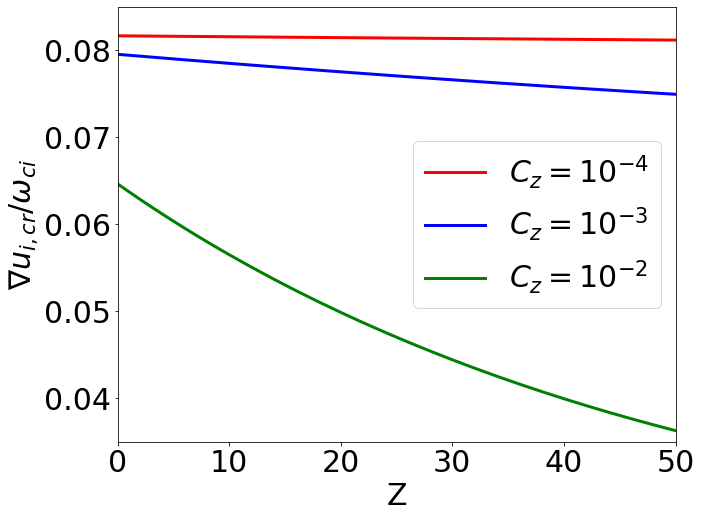
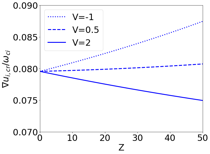
Figure 6 illustrates role of the charge number of the impurity, at fixed mass ratio (tungsten), for various impurity concentrations and various flow shear ratios . Higher can be either stabilising or destabilising depending on the parameters, such as . Here, at concentration , it is stabilising for , but destabilising for and . This stabilising role of impurities is consistent with simple intuition in the case , since impurity flow counteracts main ion flow in this case. In the case , the stabilising effect is more subtle: in this case the variation in Eq. (23) is dominated by the denominator , which can be re-written as . However, which term dominates depends on the value of . For example, for , the variation as increases is dominated by the decrease of , so increasing is stabilising. For an intermediate case, , the dependency is non-monotonous: increasing is stabilising for and destabilising for .
A more intuitive picture can be obtained by varying impurity concentration while the impurity species and are fixed.
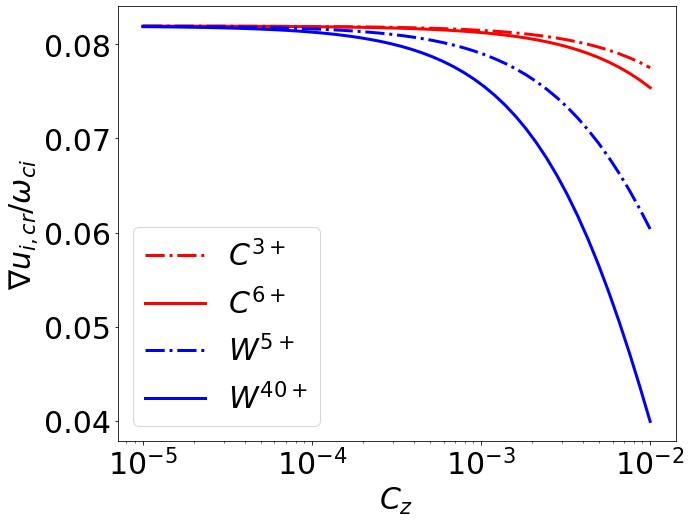
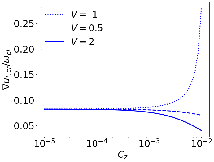
Figure 7 illustrates the role of impurity concentration, for various impurity species (C3+, C6+, W5+, W40+) and various values of . From this point of view, the role of impurity flow is consistent with simple intuition: if , impurity flow adds up to main ion flow, which is destabilising ; conversely, if , impurity flow counters main ion flow, which is stabilising. Increasing concentration accentuates the impact – whether stabilising or destabilising – of the impurity on the instability threshold.
This effect may offer new means of control of the PVG instability by impurity injection.
In summary, the critical main ion flow shear decreases nonlinearly with increasing mass ratio, and may increase or decrease in a non-trivial manner depending on all the other parameters.
For our reference case, the instability threshold is . In the next subsection, in order to study the growthrate near the instability threshold, we arbitrarily fix .
4.3 Growthrate
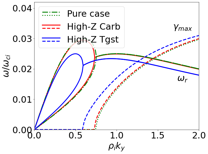
Figure 8 displays the maximum growthrate (obtained for ) against the azimuthal wavenumber, as well as the corresponding frequency, for . Here, for , the main ion parallel velocity shear is below the threshold for pure PVG. As a consequence, the behavior is qualitatively different compared to Fig. 1 (which is for , above the pure PVG threshold even for ). There is now an additional bifurcation.
Again, let us approximate the physical maximum growthrate by fixing . Then, for our plasma with , the maximum growthrate is . Consistently, the maximum growth-rate in the following figures (9, 10, 11 and 12), where impurity parameters are varied, is obtained from our model for the wave vector with components , , .
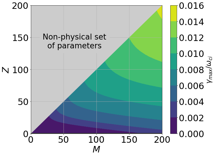
Figure 9 shows our estimated maximum growthrate against mass and charge ratio, for and . Recalling that the real frequency of the mode is typically , we confirm that our choice of cut-off () ensures that remains significantly below unity, except for unrealistically highly ionized heavy impurities. Note that here, the main ion parallel velocity shear is below the threshold for pure PVG (which is for ).
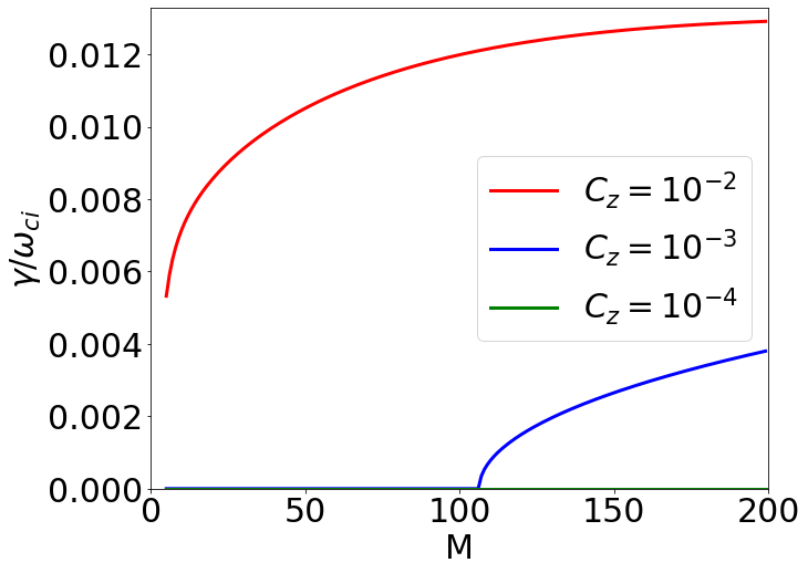
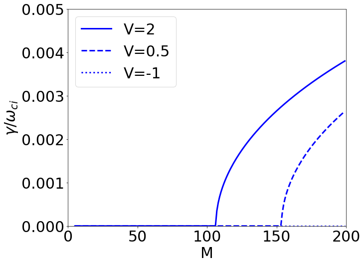
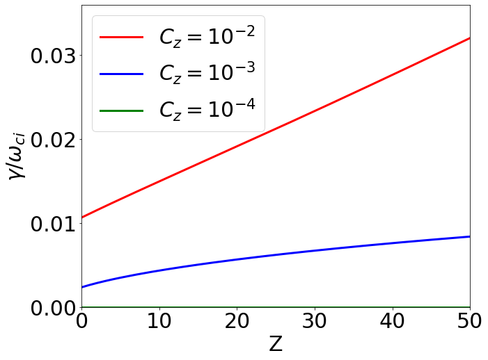
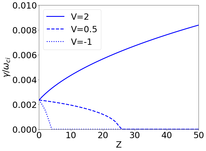
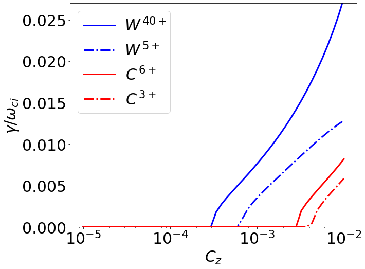
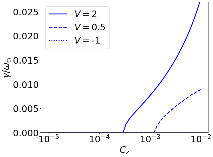
Figure 10 illustrates the role of the mass ratio on the maximum growthrate, for fixed and various and . From this perspective, the instability threshold can be viewed as a threshold in impurity mass, every other parameters being fixed. Similarly to the effect of mass on the instability threshold, increasing mass always increases the maximum growthrate.
Figure 11 illustrates the role of the impurity charge on the maximum growthrate, for fixed and various and . As a rule of thumb, the growthrate is less sensitive to than to . Increasing may be destabilising or stabilising depending on the parameters, and in particular depending on the flow shear ratio . For or , the i-PVG instability threshold can be viewed as a threshold in impurity charge, instability occuring only below a critical number.
Figure 12 illustrates the role of impurity concentration on the maximum growthrate, for various species and . In this point-of-view, the instability threshold is a threshold in concentration. With our arbitrary choice of , the concentration threshold is of the order of – for tunsgten, and of the order of – for carbon. However, with closer to , the concentration threshold can even be much lower. Here, the growthrate increases with increasing concentration. However, there are also cases where concentration has a non-monotonous impact [23].
Let us emphasize that figures 11 and 12 are useful to guide experiments which could test this theory. For example, impurities may be purposely injected in a linear device, to either excite the i-PVG, or to suppress a pure PVG (depending on the direction of flow shears). However, the analysis should be reproduced after measuring the values of parallel flows, since the thresholds in and are sensitive to the value of the main ion flow shear – and more specifically its closeness to marginal stability.
5 Conclusions and discussions
We investigated the role of a radial gradient of the parallel flow of impurities in a magnetized plasma. The linear dispersion relation indicates that the impurity-PVG is destabilised when . Similarly to the pure-PVG, the i-PVG is asymmetric in the space of wavevector components (, ): it is unstable only for .
If the plasma is unstable to the pure-PVG, then impurities can be stabilising if their flow shear is opposite to the flow shear of main ions. Note that this does not require flows themselves to be in opposite directions. The role of impurities is more prominent for higher mass and/or higher charge number. In general, the instability threshold and the growthrate are more sensitive to charge number than to mass.
The analytic expression of the maximum growthrate is given in Eq. (24). To investigate how the maximum growthrate depends on plasma and impurity parameters (Figs. 10-12), we assumed a perpendicular wavenumber comparable to the inverse Larmor radius (of main ions).
In the typical case of a hydrogen plasma with a concentration of , tungsten flow shear being twice the hydrogen flow shear, and assuming that the linear growthrate is maximum for , the i-PVG instability is unstable for hydrogen flow shear above a threshold , and most unstable for parallel wavenumbers .
Although the present work should in principle capture the main linear properties of the i-PVG, the reader should keep in mind that it is subject to several caveats: it is a local analysis, assuming cold ions and Boltzmann electrons. Our model does not include collisional effects, viscosity, resistivity. We limited our analysis to two species, but it can be straightforwardly generalised to more species.
The present work focused on the linear properties of the i-PVG. Although, the (quasi-)steady-state spectrum of fluctuations may roughly reflect the location in -space of most unstable modes, nonlinear simulations and analysis are necessary to improve predictions and understanding of steady-state fluctuations. In particular, the present work cannot address the role of zonal flows, which can be generated by PVGs [24]. Impurities may play an interesting role in both the generation and the damping of zonal flows.
Impurities are transported in the radial direction, in general by both neoclassical and turbulent processes, although one process may dominate depending on the species and plasma parameters. The efficiency of fusion depends on the radial distribution of impurities, which results from transport. For example, slight tungsten contamination of the core yields prohibitive energy losses. Therefore, it is essential to improve our understanding of impurity transport. However, the model adopted here assumes a Boltzmann response of electrons to electric fluctuations, which precludes any radial transport of electrons, and forces impurity transport to exactly balance main ion transport. This assumption is reasonable for the presented linear analysis, but is too strong for providing any conclusion about impurity transport. Relaxing this assumption is left for future work.
Acknowledgments
This work was supported by a scholarship by Kyushu University, the joint research project in RIAM, the Grants-in-Aide for Scientific Research of JSPS of Japan (JP21H01066), a grant from the Chaire Energies Durables of Ecole Polytechnique, and funding from the Agence Nationale de la Recherche for the project GRANUL (ANR-19-CE30-0005).
References
- [1] N. D’Angelo, Phys. Fluids 8, 1748 (1965).
- [2] N. D’angelo and S. V. Goeler, Phys. Fluids 9, 309 (1966).
- [3] T. Kaneko, H. Tsunoyama, and R. Hatakeyama, Phys. Rev. Lett. 90, 125001 (2003).
- [4] P. J. Catto, M. N. Rosenbluth, and C. Liu, Phys. Fluids 16, 1719 (1973).
- [5] D. McCarthy, Phys. Plasmas 9, 2451 (2002).
- [6] X. Garbet et al., Phys. Plasmas 9, 3893 (2002).
- [7] J. Drake et al., Nucl. Fusion 32, 1657 (1992).
- [8] I. Chapman, S. Brown, R. Kemp, and N. Walkden, Nucl. Fusion 52, 042005 (2012).
- [9] W. Wang et al., Nucl. Fusion 55, 122001 (2015).
- [10] S. L. Newton, S. C. Cowley, and N. F. Loureiro, Plasma Phys. Control. Fusion 52, 125001 (2010).
- [11] M. Barnes et al., Phys. Rev. Lett. 106, 175004 (2011).
- [12] A. Schekochihin, E. Highcock, and S. Cowley, Plasma Phys. Control. Fusion 54, 055011 (2012).
- [13] E. Highcock et al., Phys. Rev. Lett. 109, 265001 (2012).
- [14] A. Field et al., Rev. Sci. Instr. 83, 013508 (2012).
- [15] G. Wang et al., Plasma Phys. Control. Fusion 40, 429 (1998).
- [16] T. Kobayashi et al., Phys. Plasmas 23, 102311 (2016).
- [17] S. Inagaki et al., Sci. Rep. 6, 22189 (2016).
- [18] Y. Kosuga, S.-I. Itoh, and K. Itoh, Plasma Fusion Research 10, 3401024 (2015).
- [19] F. Brochard et al., in 49th EPS Conference on Plasma Physics (IAEA Publications, Vienna, 2023), p. THS/P5–03.
- [20] W. Guo, L. Wang, and G. Zhuang, Nucl. Fusion 59, 076012 (2019).
- [21] D. Testa et al., Phys. Plasmas 9, 243 (2002).
- [22] B. Grierson et al., Phys. Plasmas 26, 042304 (2019).
- [23] M. Lesur, J. Bourgeois, and Y. Kosuga, in Fusion Energy 2023 (Proc. 29th Int. Conf. London) (Vienna: IAEA, International Centre, 2023).
- [24] Y. Kosuga, S.-I. Itoh, and K. Itoh, Phys. Plasmas 24, 032304 (2017).