Sparse MTTKRP Acceleration for Tensor Decomposition on GPU
Abstract.
Sparse Matricized Tensor Times Khatri-Rao Product (spMTTKRP) is the bottleneck kernel of sparse tensor decomposition. In this work, we propose a GPU-based algorithm design to address the key challenges in accelerating spMTTKRP computation, including (1) eliminating global atomic operations across GPU thread blocks, (2) avoiding the intermediate values being communicated between GPU thread blocks and GPU global memory, and (3) ensuring a balanced distribution of workloads across GPU thread blocks. Our approach also supports dynamic tensor remapping, enabling the above optimizations in all the modes of the input tensor. Our approach achieves a geometric mean speedup of 1.5, 2.0, and 21.7 in total execution time across widely used datasets compared with the state-of-the-art GPU implementations. Our work is the only GPU implementation that can support tensors with modes greater than 4 since the state-of-the-art works have implementation constraints for tensors with a large number of modes.
1. Introduction
††Distribution Statement A: Approved for public release. Distribution is unlimited.Tensor Decomposition (TD) provides an intuitive method for representing multidimensional data by effectively encapsulating lower-dimensional multi-aspect structures. TD is used in various domains, including network analysis (Fernandes et al., 2020), machine learning (Cheng et al., 2020; Sidiropoulos et al., 2017; Mondelli and Montanari, 2019), and signal processing (Wen et al., 2020). Within the domain of TD, Canonical Polyadic Decomposition (CPD) has emerged as a widely used approach, with the computationally intensive Matricized Tensor Times Khatri-Rao Product (MTTKRP) being the most time-consuming kernel.
Real-world tensors often exhibit irregular shapes and nonzero value distributions, which pose significant challenges when performing spMTTKRP computations on GPU. These challenges arise from irregular memory access patterns, load imbalances among a large number of GPU threads, and the synchronization overhead associated with performing atomic operations.
Recent efforts have proposed mode-agnostic tensor optimizations to address these issues by maintaining a single tensor copy, distributing spMTTKRP computations across GPU threads, and optimizing load balancing for the overall computation (Li et al., 2018a). However, these implementations use global atomic operations, which introduce a considerable synchronization latency between streaming multiprocessors. Additionally, these approaches increase the demands on external memory since they store the intermediate computation results in GPU global memory for future use. It introduces challenges in scalability, limiting the applicability of these approaches. As the size of the tensor increases, there is a looming risk of memory explosion, further exacerbating the scalability problem. To accommodate the irregular data access patterns inherent in each tensor mode, proposed tensor formats in the literature rely on multiple copies, often called mode-specific tensor formats (Nisa et al., 2019c, a; Liu et al., 2017; Phipps and Kolda, 2019) where mode-specific optimizations are used in each tensor copy. However, replicating the original tensor across different permutations of nonzero tensor elements becomes impractical as the number of modes grows. In this paper, we compare our work against state-of-the-art mode-agnostic and mode-specific implementations as discussed in Section 5.1.4 and Section 5.6.
In our prior work (Wijeratne et al., 2023b), we have introduced FLYCOO, a tensor format tailored to accelerate spMTTKRP on Field Programmable Gate Arrays (FPGAs). FLYCOO optimizes data locality across all tensor modes when accessing the input tensor and factor matrices within the FPGA external memory. Furthermore, (Wijeratne et al., 2023b) proposes a dynamic tensor remapping technique that is performed during execution. This strategic tensor reordering reduces inter-processor dependencies during elementwise computations. Moreover, this approach eliminates the need for multiple tensor copies corresponding to the number of tensor modes and mitigates memory explosion arising from the large number of intermediate values generated during the execution.
In this paper, we adopt and refine the FLYCOO format to create a parallel algorithm tailored for GPUs, effectively obviating the necessity for specialized hardware. We introduce GPU-specific optimizations, facilitating load-balanced computation across GPU Streaming Multiprocessors (SMs) without global atomic operations.
The key contributions of this work are:
-
•
We introduce a novel parallel algorithm to perform spMTTKRP on GPU. Our algorithm eliminates the intermediate value communication across GPU thread blocks. It achieves 2.3 higher L1-cache throughput during the execution time compared with the state-of-the-art.
-
•
We introduce dynamic tensor remapping on GPU to reorder the tensor during runtime, enabling mode-specific optimizations to the tensor format. These optimizations lead to 1.2 - 1.9 higher streaming multiprocessor throughput compared with the state-of-the-art.
-
•
We map our proposed parallel algorithm to GPU thread blocks where each thread block can concurrently execute spMTTKRP elementwise computation without global atomic operations and perform dynamic tensor remapping without atomic operations among GPU threads.
-
•
Our approach achieves a geometric mean speedup of 1.5 and 2.0 in total execution time compared with the baselines with mode-specific optimizations. Our work also shows a geometric mean speedup of 21.7 in execution time compared with the state-of-the-art mode-agnostic implementations.
2. Background and Related Work
2.1. Introduction to Tensors
A tensor is a generalization of an array to multiple dimensions. In the simplest high-dimensional case, a tensor is a three-dimensional array, which can be visualized as a data cube. For a thorough review of tensors, refer to (Kolda and Bader, 2009). Table 1 summarizes the tensor notations.
| Symbol | Details |
|---|---|
| vector outer product | |
| Kronecker product | |
| Khatri-Rao product | |
| matrix | |
| vector | |
| scalar | |
| sparse tensor | |
| mode- matricization of |
2.1.1. Tensor mode
In Tensor Decomposition, the number of dimensions of an input tensor is commonly called the number of tensor modes. For example, a vector can be seen as a mode-1 tensor. A -mode, real-valued tensor is denoted by . This paper focuses on tensors of mode three or higher for tensor decomposition.
2.1.2. Indices of a nonzero tensor element
For a 3-mode tensor, , a nonzero tensor element is indicated as . Here, , , and are the positions or coordinates of in the tensor , which are commonly referred to as indices of the tensor element.
2.1.3. Tensor matricization
denotes the mode- matricization or matrix unfolding (Favier and de Almeida, 2014) of . is defined as the matrix where the parenthetical ordering indicates, the mode- column vectors are arranged by sweeping all the other mode indices through their ranges.
2.1.4. Canonical Poliyedic Tensor Decomposition (CPD)
CPD decomposes into a sum of single-mode tensors (i.e., arrays), which best approximates . For example, given a 3-mode tensor , our goal is to approximate the original tensor as , where is a positive integer and , , and .
For each of the three modes, the spMTTKRP operation can be expressed as
| (1) |
The alternating least squares (ALS) method is used to compute CPD. In a 3-mode tensor, CPD sequentially performs the computations in Equation 1, iteratively. This can be generalized to higher mode tensors. Note that the matricization of is different for each factor matrix computation. In this paper, performing MTTKRP on all the matricizations of an input tensor is called computing MTTKRP along all the modes. The outputs , , and are the factor matrices that approximate . , , and refers to the column of , , and , respectively.
In this paper, we focus on MTTKRP on sparse tensors (spMTTKRP), which means the tensor is sparse. Note however, that the factor matrices are dense.
2.1.5. Elementwise computation
The focus of this paper is to reduce the total execution time of spMTTKRP along all the modes of the tensor. Efficiently performing the elementwise computation is described below.
Figure 1 summarizes the elementwise computation of a nonzero tensor element in mode 2 of a tensor with 3 modes.
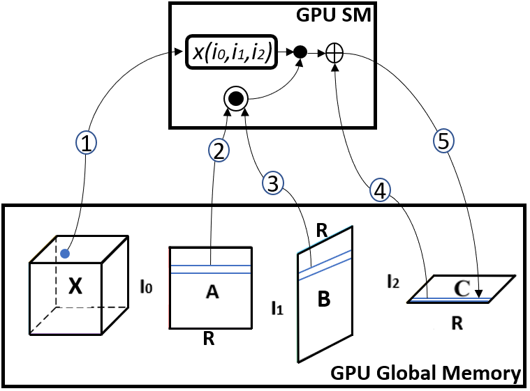
In Figure 1, the elementwise computation is carried out on a nonzero tensor element, denoted as . In sparse tensors, is typically represented in formats such as COOrdinate (COO). These formats store the indices (, , and ) along with the element value (i.e., ).
To perform the computation, is first loaded onto the processing units (i.e., streamings multiprocessors for GPU) from the external memory (Step 1). The compute device retrieves the rows , , and from the factor matrices using the index values extracted from (Step 2, Step 3, and Step 4). Then the compute device performs the following computation:
Here, refers to the column index of a factor matrix row (). The operation involves performing a Hadamard product between row and row , and then multiplying each element of the resulting product by . Finally, the updated value is stored in the external memory (Step 5).
2.2. Related Work
A. Nguyen et al. (Nguyen et al., 2022a) propose the Blocked Linearized CoOrdinate (BLCO) format that enables efficient out-of-memory computation of tensor algorithms using a unified implementation that works on a single tensor copy. In contrast to BLCO, we use a dynamic tensor format that can be used to reorder the tensor during runtime. Our work also does not require a conflict resolution algorithm like BLCO that can introduce additional overhead to the overall execution time.
I. Nisa et al. (Nisa et al., 2019c, a) propose a novel tensor format to distribute the workload among GPU threads. This work requires multiple tensor copies to perform spMTTKP along all the modes of the input tensor. Unlike (Nisa et al., 2019c, a), our work employs a dynamic tensor remapping technique to optimize data locality during elementwise computation and eliminate the global atomic operations.
J. Li et al. (Li et al., 2018a) introduce a GPU implementation employing HiCOO (Li et al., 2018b) tensor format to accelerate spMTTKRP. Their approach incorporates a block-based format with compression techniques to handle sparse tensors efficiently. Compared with (Li et al., 2018a), our work reduces the intermediate value communication to the GPU global memory with a novel tensor format and introduces a novel tensor partitioning scheme to load balance the total computations among GPU SMs.
In our prior work (Wijeratne et al., 2023b), we developed a custom accelerator design targeted for Field Programmable Gate Array (FPGA) to perform spMTTKRP on sparse tensors. We introduce a specialized tensor format called FLYCOO, which supports custom hardware-specific optimizations. We also adopted the FLYCOO tensor format to perform spMTTKRP on multi-core CPU (Wijeratne et al., 2023a). However, it is important to note that tackling spMTTKRP on a GPU presents a unique set of challenges compared to FPGA and CPU architectures. In this work, we adapt the FLYCOO format and propose GPU-specific optimizations, including ensuring a balanced distribution of workloads across GPU thread blocks, eliminating global atomic operations across GPU thread blocks, and avoiding the intermediate values being communicated across GPU thread blocks.
3. Optimizing Tensor Format for GPU
In this paper, we develop a GPU-specific dynamic tensor remapping based on adapting the mode-agnostic tensor format FLYCOO (Wijeratne et al., 2023b). In this Section, we first introduce the dynamic tensor remapping used in FLYCOO. After that, we briefly summarize the novelty of our work following the notion of hypergraph representation of a tensor and then use it to describe our dynamic tensor remapping strategy for GPUs.
In the following, When performing spMTTKRP for mode of a tensor, we denote mode as the output mode and its corresponding factor matrix as the output factor matrix. The rest of the tensor modes are called input modes, and the corresponding factor matrices are called input factor matrices.
3.1. Dynamic Tensor Remapping
Dynamic tensor remapping involves reordering nonzero tensor elements at runtime based on the next mode in which spMTTKRP is performed.
Initially, the tensor is ordered based on the indices of mode 0. As the spMTTKRP computation proceeds for mode 0, the tensor is dynamically reordered according to the indices of mode 1. Consequently, when the computation for mode 1 begins, the tensor is already ordered according to the indices of mode 1.
3.2. Modified FLYCOO Tensor Format
We refine the tensor element representation by introducing a novel remap ID scheme that can perform dynamic tensor remapping on each nonzero tensor element independently of each other (see Section 3.5). Hence, it avoids atomic operations among GPU threads while performing dynamic tensor remapping(see Observation 1).
We also introduce a SM-based tensor partitioning scheme that load balances the total computations among the GPU SMs (see Section 3.4). It reduces the idle time of SMs, resulting in higher overall GPU compute throughput.
3.3. Hypergraph Representation
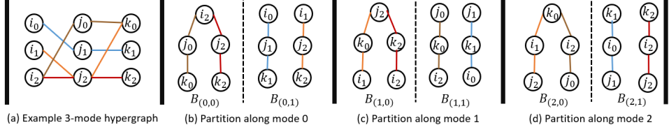
For a mode tensor , with nonzero elements, we consider the hypergraph, with vertex set and each nonzero tensor element in being represented as a hyperedge in . Here, is the set of all the indices in mode and . Figure 3 shows an example hypergraph representation of a 3-mode tensor.
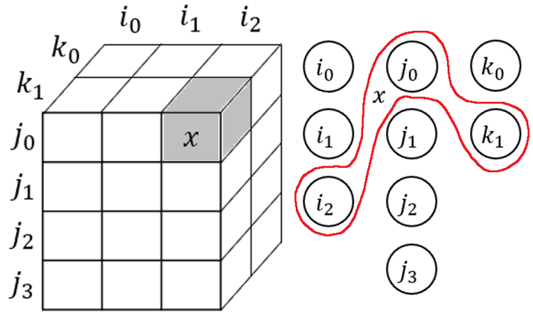
Observe that (Ref. Section 2.1.5) when computing spMTTKRP for a row in factor matrix of mode (the output mode), elementwise computations are performed on the nonzero tensor elements with the same mode index (Ref. Section 2.1.2) as the mode factor matrix row. In the hypergraph representation, the computation of the output factor matrix of mode involves performing elementwise operations on all the hyperedges connected to the same vertex in mode of the tensor. Hence, we propose a partitioning scheme that brings all the hyperedges connected to the same output mode vertex into the same partition. Doing so allows each tensor partition to be executed without dependencies among tensor partitions while updating the output values.
3.4. Tensor Partitioning Scheme
Following the notation introduced in Section 3.3, consider the input tensor and its corresponding hypergraph representation where is partitioned into tensor partitions along each mode. In , for a given mode , the vertices in are ordered based on the number of hyperedges in incident on each vertex. Let us denote the ordered vertex set for mode as . Subsequently, we iterate through the ordered list, , vertex by vertex, and assign each vertex to a partition in a cyclic fashion. This step effectively partitions the vertices in mode among the tensor partitions. Next, we collect all the hyperedges incident on each tensor partition. We denote these hyperedges that map to partition as Partition ID where . Once the partitioning is complete, we order the hyperedges based on the partition IDs (i.e., ) and assign a remap id, to each hyperedge, reflecting its position within the overall tensor. This entire process is repeated for all the modes of the hypergraph. Algorithm 1 summarizes the tensor partitioning scheme.
Figure 2 demonstrates a partitioning scheme for an example hypergraph with 4 hyperedges and 3 vertices along each mode and . In the Figure, different hyperedges are represented by lines with different colors. In mode 0, vertex is incident to 2 hyperedges, while vertices and each have a single hyperedge incident to them. Following the partitioning scheme outlined in Algorithm 1, we assign hyperedges incident to to partition 0 of mode 0 (i.e., ) and hyperedges incident to and to . In this configuration, each partition of mode 0 contains 2 hyperedges. This process is similarly used for the remaining modes, as shown in Figure 2.
3.4.1. Load Balancing
3.5. Tensor Element Representation
Using the FLYCOO tensor format in (Wijeratne et al., 2023b) and the proposed tensor partitioning scheme in Section 3.4, a tensor can be represented as a sequence , where each element is a tuple , , . Here, represents a vector of remap ids based on the position of in each output tensor mode and represents a vector of indices of in each mode (see Section 2.1.2).
3.5.1. Memory Requirements
Following the tensor element representation, a tensor element is a tuple , , . A single nonzero element in the FLYCOO format requires bits, where is the number of bits needed to store the floating-point value of the nonzero tensor element. Here, , , and .
4. Parallel Algorithm
4.1. Elementwise Computation on GPU
Algorithm 2 describes the elementwise computation carried out on each nonzero tensor element. In Algorithm 2, the rows of the input factor matrices are loaded from GPU global memory (Algorithm 2: lines 9-10) depending on the indices of the current tensor element () that is being executed in the GPU thread. Each GPU thread block locally updates the output factor matrix (Algorithm 2: lines 15) while each thread inside the thread block maintains the coherency to ensure the correctness of the program. The elementwise computation between the tensor element and the rows of the input factor matrices (Algorithm 2, lines 9-15) is the same as in Section 2.1.5.
4.2. Dynamic Tensor Remapping on GPU
Algorithm 3 shows executing dynamic tensor remapping on a nonzero tensor element. As described in Section 3.1, dynamic tensor remapping reorders the tensor during execution time to support the spMTTKRP computation along the subsequent mode. Algorithm 3 shows the dynamic tensor remapping performed during mode elementwise computation. Hence, Algorithm 3 remap the tensor according to the remap ids of mode to support the spMTTKRP computation along the subsequent mode mod . The reordered nonzero tensor elements are collected in the tensor copy, (Algorithm 3: line 6). With the proposed tensor partitioning scheme in Section 3.4, all the threads in a GPU thread block that perform dynamic tensor remapping can independently operate on nonzero elements, avoiding atomic operations among the GPU threads as demonstrated in Observation 1.
4.3. Parallel Algorithm Mapping to GPU Thread Blocks
The basic computing unit of a GPU is a thread. According to the GPU programming model, a multi-threaded program is partitioned into blocks of threads (i.e., thread blocks) that operate independently. Thread blocks are organized into a multi-dimensional grid. For a thorough overview of the GPU programming model, please refer to (Ansorge, 2022; Zeller, 2011).
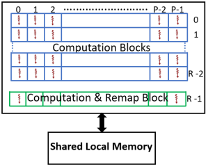
We propose a GPU implementation where GPU thread blocks can perform Elementwise Computation (i.e., Algorithm 2) and Dynamic Tensor Remapping (i.e., Algorithm 3). Figure 4 shows a thread block with the dimensions of , where denotes the rank of the factor matrices and indicates the number of nonzero tensor elements parallelly loaded to a thread block. In Figure 4, each thread corresponds to a distinct square within the thread block. Each column of the thread block shares the same nonzero tensor element. In the Figure 4, we indicate the threads that only perform the elementwise computation in blue and the threads that perform elementwise computation with dynamic tensor remapping in green.
Algorithm 4 outlines the computations executed on each GPU thread block. In Algorithm 4, corresponds to tensor partition in mode (see Section 3.4). When a GPU SM is idle, a thread block and its corresponding tensor partition are assigned to the SM for computation. Once a tensor partition is assigned for computation, the thread block performs elementwise spMTTKRP computation and dynamic tensor remapping on the assigned partition. Each column in the thread block loads a single nonzero tensor element at a time and shares it across the threads in the same column. Each thread column extracts the embedded information from the loaded nonzero tensor element (Algorithm 4: line 12-15). Subsequently, each thread block performs elementwise computation (Algorithm 4: line 17). Only the last row () of the thread block performs dynamic tensor remapping (Algorithm 4: line 18-19) on each loaded tensor element. To achieve threadwise parallelism in elementwise computation, each thread in a column only executes the computations on its corresponding rank (Algorithm 2: line 12 - 15).
According to Algorithm 4, the dynamic tensor remapping and the elementwise computation update data in the memory during the execution time. Since there are multiple thread blocks operating in parallel, the threads should not cause any race conditions while updating the data to maintain the correctness of the program. In our work, we avoid race conditions in dynamic tensor remapping and elementwise computation as follows:
(1) Dynamic tensor remapping: GPU threads in all the thread blocks update different locations of tensor copy during the execution time using the unique remap IDs embedded in nonzero tensor elements as discussed in Section 3.4. It leads to avoiding atomic operations in the implementation during dynamic tensor remapping (See Observation 1). Atomic operations are used to prevent race conditions between threads in the same thread block or different thread blocks (Nishitsuji, 2023; Cook, 2012), which leads to synchronization overheads.
(2) spMTTKRP elementwise computation: During the spMTTKRP elementwise computation, multiple threads can simultaneously update the same row of the output factor matrix. Therefore, we need atomic operations among the threads, ensuring the correctness of spMTTKRP elementwise computation. Since each tensor partition is assigned to a single thread block, the proposed Algorithm 4 eliminates the need for global atomic operations among GPU thread blocks (See Observation 2). Global atomic operations are used to prevent conflicts while updating values between threads in different thread blocks (Nishitsuji, 2023; Cook, 2012). Global atomic operations lead to significant synchronization overhead among threads in different GPU thread blocks.
Observation 1.
For a mode input tensor in FLYCOO format, the GPU threads can perform dynamic tensor remapping for each mode () without atomic operations among any GPU threads.
Proof: According to the FLYCOO tensor representation discussed in Section 3.5, we define as , representing a nonzero tensor element, each has a distinct remap id, denoted as , which denotes the location of in during the dynamic tensor remapping process. As per the tensor partitioning scheme defined in Section 3.4, it is guaranteed that is a unique remap ID for in mode . Consequently, the thread responsible for dynamic tensor remapping of can independently perform at the location without interference from other GPU threads. Given that this condition holds for all , dynamic tensor remapping for tensor can be executed without the need for atomic operations.
Observation 2.
Elementwise computations of spMTTKRP can be performed without global atomic operations among GPU thread blocks.
Proof: Consider tensor element where is a partition of the input tensor in mode . Let the index of in mode be where update the row of output factor matrix of mode during the elementwise computation. Consequently, race conditions for can only occur with threads that execute nonzero tensor elements with index . According to the tensor partitioning scheme described in Section 3.4, all the tensor elements with index are in . Since all the nonzero tensor elements of tensor partition are executed on a single thread block, race conditions corresponding to row only occur inside the same thread block. Thus, there is no need for global atomic operations between GPU thread blocks while executing elementwise computation on . Given that this condition holds for all , there is no need for global atomic operations among GPU thread blocks during spMTTKRP elementwise computation.
4.4. Overall Algorithm
Algorithm 5 shows the overall parallel Algorithm for performing spMTTKRP along all the modes of an input tensor on GPU. Algorithm 5 takes (1) which is an input tensor ordered according to , and (2) factor matrices denoted as .
As shown in Algorithm 5, the spMTTKRP is performed mode by mode (Algorithm 5: line 7). Within each mode, each thread block (Algorithm 5: line 9) executes a tensor partition mapped to it. At the end of all the computations of a mode, the GPU is globally synchronized before the next mode’s computations to maintain the correctness of the program (Algorithm 5: line 10). Since we perform dynamic tensor remapping, holds a tensor copy ordered according to the next mode to be computed at the end of each mode computation. Hence, the memory pointers to each tensor copy are swapped, preparing them for the subsequent mode computation (Algorithm 5: line 12).
5. Experimental Results
5.1. Experimental Setup
5.1.1. Platforms
We conduct experiments on the NVIDIA RTX 3090, featuring the Ampere architecture. The platform has 82 Streaming Multiprocessors (SMs) and 10496 cores running at 1.4 GHz, sharing 24 GB of GDDR6X global memory. Table 2 shows the details of the platform.
| Frequency | 1695 MHz |
|---|---|
| Peak Performance | 35.6 TFLOPS |
| On-chip Memory | 6 MB L2 Cache |
| Memory Bandwidth | 936.2 GB/s |
We use a 2-socket AMD Ryzen Threadripper 3990X CPU with 32 physical cores (64 threads) running at 2.2 GHz, sharing 256 GB of external CPU memory for preprocessing the input tensors.
5.1.2. Implementation
5.1.3. Datasets
We use tensors from the Formidable Repository of Open Sparse Tensors and Tools (FROSTT) dataset (Smith et al., 2017) and Recommender Systems and Personalization Datasets (He and McAuley, 2016; Bollacker et al., 2008; Rappaz et al., 2021; McAuley, 2021). Table 3 summarizes the characteristics of the tensors.
5.1.4. Baselines
We evaluate the performance of our work by comparing it with the state-of-the-art GPU implementations: BLCO (Nguyen et al., 2022a), MM-CSF (Nisa et al., 2019c), and ParTI-GPU (Li et al., 2018a). To achieve optimal results with ParTI-GPU, we use the recommended configurations provided in the source code (Li et al., 2019). For our experiments, we utilize the open-source BLCO repository (Nguyen et al., 2022b), ParTI repository (Li et al., 2019), and MM-CSF (Nisa et al., 2019b) repository. The BLCO (Nguyen et al., 2022a) repository allows running MTTKRP mode-by-mode (i.e., mode-specific MTTKRP) where the input tensor is ordered specific to the given mode before running MTTKRP on GPU (Nguyen et al., 2022b).
5.1.5. Default Configuration
We use RTX 3090 with , , and as our configuration for conducting the experiments.
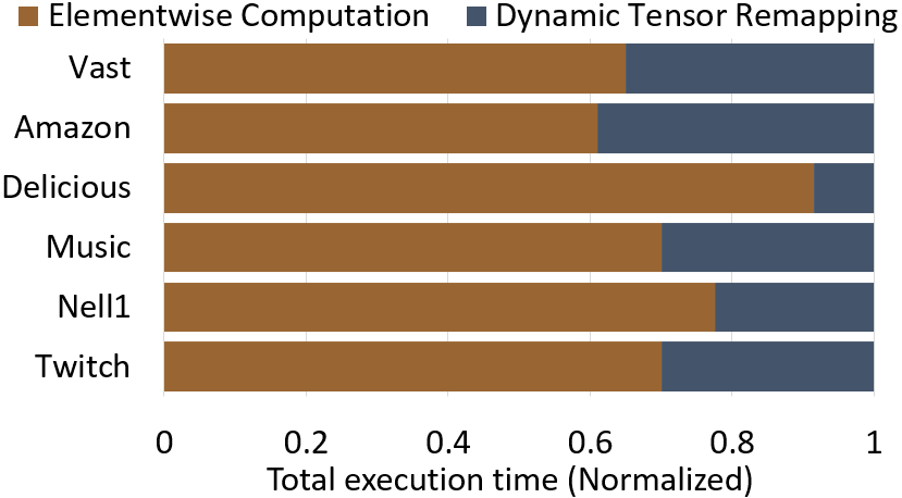
5.2. Performance of Dynamic Remapping
Figure 5 shows a detailed breakdown of the total execution time (normalized) between elementwise computation and dynamic tensor remapping. To determine the execution time of elementwise computations in each mode, we use a mode-specific tensor copy for the computations in that mode where each tensor copy is in FLYCOO format and ordered according to the remap id (see Section 3.4) of the corresponding mode.
5.3. Compute SM Throughput
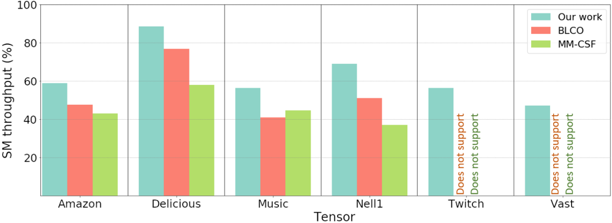
Compute SM throughput is a commonly used metric introduced by NVIDIA Nsight Compute (Iyer and Kiel, 2016) for GPU to report the utilization achieved by the SMs while executing a kernel with respect to the theoretical maximum utilization of the selected GPU (Iyer and Kiel, 2016). NVIDIA Nsight Compute provides the achieved throughput of the kernel as a percentage value.
Figure 6 compares the SM throughput of our work for each dataset against the state-of-the-art. We use NVIDIA Nsight Compute to measure the throughput, as mentioned above. In all the datasets, our work shows 1.2 - 1.4 and 1.3 - 2.0 higher compute throughput than BLCO and MM-CSF, respectively. Our work shows higher throughout due to the minimum SM idle time of the proposed load balancing scheme and eliminating the intermediate results communication between the SMs. Since the baselines do not support tensors with a large number of modes, we could not report the SM throughput values for BLCO and MM-CSF on Twitch and Vast.
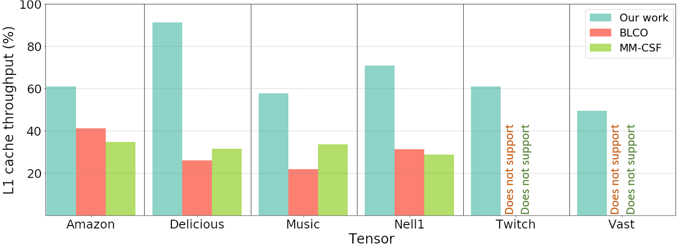
5.4. L1 Cache Throughput
L1 cache throughput is defined as the sustained memory throughput between all the L1 caches and their connected SMs as a percentage of the maximum theoretical throughput that can be achieved (NVIDIA, 2023) during the execution time of a kernel. We use NVIDIA Nsight Compute to evaluate the L1 cache throughput. Figure 7 shows the L1 cache throughput comparison of our work against the baselines. In all the datasets, our work shows 1.5 - 2.7 and 1.7 - 3.0 higher L1 cache throughput compared with BLCO and MM-CSF. This is due to the significant amount of data in the L1 cache being reused during the execution time.
5.5. Impact of Algorithm to GPU Block Mapping
In our work, we map our computational model onto the GPU thread block. The number of columns in the thread block is set to match the parallel loading of nonzero tensor elements (). Figure 8 illustrates the impact of varying on SM throughput for . In our thread block design, R equals the number of rows in a thread block (see Section 4.3).
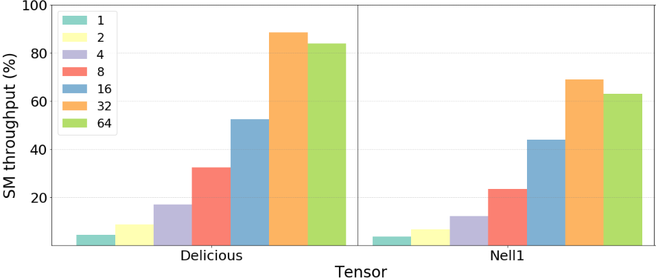
We observe a linear increase in throughput as increases from to . However, for , a decrease in throughput is noted due to multiple elementwise computations associated with different columns of the output factor matrix map into the same row of the thread block. Note that each thread block of the RTX 3090 GPU accommodates 1024 threads. Hence, keeping distributes the elementwise computations among the threads (i.e., , when and ), optimally. It is consistent across all the tensors. Therefore, we set the parameter value .
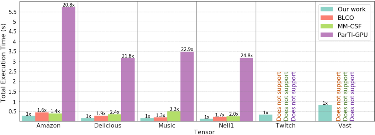
Figure 9 shows the total execution time of our work and the baselines on the RTX 3090. The corresponding speedup achieved by our work over each baseline is displayed at the top of the respective bar. Similar to the baselines (Nguyen et al., 2022a; Nisa et al., 2019c; Li et al., 2018a), we set the rank of the factor matrices () to 32. Our work demonstrates a geometric mean of 1.5, 2.0, and 21.7 in speedup compared to BLCO, MM-CSF, and ParTI-GPU. Table 4 summarizes the overall speedup achieved by our approach compared to each baseline.
It is worth noting that MM-CSF operates as a mode-specific implementation, necessitating multiple copies of the tensor during execution. BLCO’s implementation involves ordering the tensor at the beginning of each mode computation and optimizing the input tensor for efficient execution of the specific mode. These overheads of MM-CSF and BLCO are not considered in the reported timings in Figure 9. Note that our work considers dynamic remapping overhead.
5.6. Overall Performance
Our work stands out as the only GPU implementation capable of executing large tensors with a higher number of modes, such as Twitch and Vast. In contrast, BLCO, MM-CSF, and ParTI-GPU lack support for tensors with the number of modes greater than 4.
Our work avoids communicating intermediate values among SMs and between SMs and GPU global memory. These intermediate values are stored in the L1 cache and reused with high L1 cache throughput (see Figure 7). Also, our load-balancing scheme improves the overall SM throughput, reducing the idle time of the GPU SMs.
5.7. Preprocessing Time
The preprocessing of an input tensor involves generating tensor partitions and converting the tensor into FLYCOO format by representing a nonzero tensor element in FLYCOO tensor element representation. To accelerate this process, we use OpenMP (Chandra, 2001) and Boost library (Schäling, 2014).
Although this work does not focus on the accelerating preprocessing time, we have included a comparison of preprocessing times in Figure 10 for the sake of completeness. For the comparison, we use the baselines that report their preprocessing time. The CPU configuration used for preprocessing can be found in Section 5.1.1.
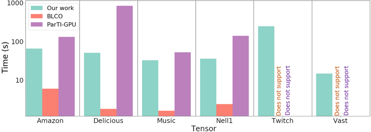
Our preprocessing is faster than ParTI-GPU as our preprocessing approach only looks at the nonzero tensor elements during partitioning. In contrast, the ParTI-GPU partitioning scheme (Li et al., 2018a) spans the entire index space across all the modes of a tensor, which is much larger than the number of nonzero tensor elements.
As described in Section 3.4, we partition the tensor along all the modes. BLCO (Nguyen et al., 2022a) partitions the tensor once before executing spMTTKRP along a specific mode. Hence, BLCO preprocesses the tensor faster than our work. Note that we compare the preprocessing time of BLCO to order the tensor for a single mode.
6. Conclusion and Future Work
This paper introduced a parallel algorithm design for GPUs to accelerate spMTTKRP across all the modes of an input tensor. The experimental results demonstrate that Our approach achieves a geometric mean speedup of 1.5 and 2.0 in total execution time compared with the state-of-the-art mode-specific implementations and 21.7 geometric mean speedup with the state-of-the-art mode-agnostic implementations.
Our future work focuses on adapting the proposed parallel algorithm on heterogeneous computing platforms. It will ensure that our work can be effectively applied across various hardware.
ACKNOWLEDGEMENT
This work is supported by the National Science Foundation (NSF) under grant CNS-2009057 and in part by DEVCOM Army Research Lab under grant W911NF2220159.
References
- (1)
- Ansorge (2022) Richard Ansorge. 2022. Programming in parallel with CUDA: a practical guide. Cambridge University Press.
- Bollacker et al. (2008) Kurt Bollacker, Colin Evans, Praveen Paritosh, Tim Sturge, and Jamie Taylor. 2008. Freebase: A Collaboratively Created Graph Database for Structuring Human Knowledge. In Proceedings of the 2008 ACM SIGMOD International Conference on Management of Data (Vancouver, Canada) (SIGMOD ’08). Association for Computing Machinery, New York, NY, USA, 1247–1250. https://doi.org/10.1145/1376616.1376746
- Chandra (2001) Rohit Chandra. 2001. Parallel programming in OpenMP. Morgan kaufmann.
- Cheng et al. (2020) Zhiyu Cheng, Baopu Li, Yanwen Fan, and Yingze Bao. 2020. A novel rank selection scheme in tensor ring decomposition based on reinforcement learning for deep neural networks. In ICASSP 2020-2020 IEEE International Conference on Acoustics, Speech and Signal Processing (ICASSP). IEEE, 3292–3296.
- Cook (2012) Shane Cook. 2012. CUDA programming: a developer’s guide to parallel computing with GPUs. Newnes.
- Fatica (2008) Massimiliano Fatica. 2008. CUDA toolkit and libraries. In 2008 IEEE hot chips 20 symposium (HCS). IEEE, 1–22.
- Favier and de Almeida (2014) Gérard Favier and André LF de Almeida. 2014. Overview of constrained PARAFAC models. EURASIP Journal on Advances in Signal Processing 2014, 1 (2014), 1–25.
- Fernandes et al. (2020) Sofia Fernandes, Hadi Fanaee-T, and João Gama. 2020. Tensor decomposition for analysing time-evolving social networks: An overview. Artificial Intelligence Review (2020), 1–26.
- Graham (1969) Ronald L. Graham. 1969. Bounds on multiprocessing timing anomalies. SIAM journal on Applied Mathematics 17, 2 (1969), 416–429.
- He and McAuley (2016) Ruining He and Julian McAuley. 2016. Ups and Downs: Modeling the Visual Evolution of Fashion Trends with One-Class Collaborative Filtering. In Proceedings of the 25th International Conference on World Wide Web (Montréal, Québec, Canada) (WWW ’16). International World Wide Web Conferences Steering Committee, Republic and Canton of Geneva, CHE, 507–517. https://doi.org/10.1145/2872427.2883037
- Iyer and Kiel (2016) Kumar Iyer and Jeffrey Kiel. 2016. GPU debugging and Profiling with NVIDIA Parallel Nsight. Game Development Tools (2016), 303–324.
- Kolda and Bader (2009) Tamara G Kolda and Brett W Bader. 2009. Tensor decompositions and applications. SIAM review 51, 3 (2009), 455–500.
- Li et al. (2018a) Jiajia Li, Yuchen Ma, and Richard Vuduc. 2018a. ParTI!: A parallel tensor infrastructure for multicore CPUs and GPUs. A parallel tensor infrastructure for multicore CPUs and GPUs (2018).
- Li et al. (2018b) Jiajia Li, Jimeng Sun, and Richard Vuduc. 2018b. HiCOO: Hierarchical Storage of Sparse Tensors. In SC18: International Conference for High Performance Computing, Networking, Storage and Analysis. 238–252. https://doi.org/10.1109/SC.2018.00022
- Li et al. (2019) Jiajia Li, Bora Uçar, Ümit V. Çatalyürek, Jimeng Sun, Kevin Barker, and Richard Vuduc. 2019. Efficient and Effective Sparse Tensor Reordering. https://github.com/hpcgarage/ParTI
- Liu et al. (2017) Bangtian Liu, Chengyao Wen, Anand D. Sarwate, and Maryam Mehri Dehnavi. 2017. A Unified Optimization Approach for Sparse Tensor Operations on GPUs. In 2017 IEEE International Conference on Cluster Computing (CLUSTER). 47–57. https://doi.org/10.1109/CLUSTER.2017.75
- McAuley (2021) Julian McAuley. 2021. Recommender Systems and Personalization Datasets. https://cseweb.ucsd.edu/~jmcauley/datasets.html#
- Mondelli and Montanari (2019) Marco Mondelli and Andrea Montanari. 2019. On the connection between learning two-layer neural networks and tensor decomposition. In The 22nd International Conference on Artificial Intelligence and Statistics. PMLR, 1051–1060.
- Nguyen et al. (2022a) Andy Nguyen, Ahmed E. Helal, Fabio Checconi, Jan Laukemann, Jesmin Jahan Tithi, Yongseok Soh, Teresa Ranadive, Fabrizio Petrini, and Jee W. Choi. 2022a. Efficient, out-of-Memory Sparse MTTKRP on Massively Parallel Architectures. In Proceedings of the 36th ACM International Conference on Supercomputing (Virtual Event) (ICS ’22). Association for Computing Machinery, New York, NY, USA, Article 26, 13 pages. https://doi.org/10.1145/3524059.3532363
- Nguyen et al. (2022b) Andy Nguyen, Ahmed E Helal, Fabio Checconi, Jan Laukemann, Jesmin Jahan Tithi, Yongseok Soh, Teresa Ranadive, Fabrizio Petrini, and Jee W Choi. 2022b. Efficient, out-of-memory sparse MTTKRP on massively parallel architectures. https://github.com/jeewhanchoi/blocked-linearized-coordinate
- Nisa et al. (2019a) Israt Nisa, Jiajia Li, Aravind Sukumaran-Rajam, Prasant Singh Rawat, Sriram Krishnamoorthy, and P. Sadayappan. 2019a. An Efficient Mixed-Mode Representation of Sparse Tensors. In Proceedings of the International Conference for High Performance Computing, Networking, Storage and Analysis (Denver, Colorado) (SC ’19). Association for Computing Machinery, New York, NY, USA, Article 49, 25 pages. https://doi.org/10.1145/3295500.3356216
- Nisa et al. (2019b) Israt Nisa, Jiajia Li, Aravind Sukumaran-Rajam, Prasant Singh Rawat, Sriram Krishnamoorthy, and Ponnuswamy Sadayappan. 2019b. An Efficient Mixed-Mode Representation of Sparse Tensors. https://github.com/isratnisa/MM-CSF
- Nisa et al. (2019c) Israt Nisa, Jiajia Li, Aravind Sukumaran-Rajam, Richard Vuduc, and P. Sadayappan. 2019c. Load-Balanced Sparse MTTKRP on GPUs. In 2019 IEEE International Parallel and Distributed Processing Symposium (IPDPS). 123–133. https://doi.org/10.1109/IPDPS.2019.00023
- Nishitsuji (2023) Takashi Nishitsuji. 2023. Basics of OpenCL. In Hardware Acceleration of Computational Holography. Springer, 83–95.
- NVIDIA (2023) NVIDIA. 2023. DEVELOPER TOOLS Documentation. https://docs.nvidia.com/nsight-compute/ProfilingGuide/index.html#
- Phipps and Kolda (2019) Eric T. Phipps and Tamara G. Kolda. 2019. Software for Sparse Tensor Decomposition on Emerging Computing Architectures. SIAM Journal on Scientific Computing 41, 3 (2019), C269–C290. https://doi.org/10.1137/18M1210691 arXiv:https://doi.org/10.1137/18M1210691
- Rappaz et al. (2021) Jérémie Rappaz, Julian McAuley, and Karl Aberer. 2021. Recommendation on Live-Streaming Platforms: Dynamic Availability and Repeat Consumption. In Proceedings of the 15th ACM Conference on Recommender Systems (Amsterdam, Netherlands) (RecSys ’21). Association for Computing Machinery, New York, NY, USA, 390–399. https://doi.org/10.1145/3460231.3474267
- Schäling (2014) Boris Schäling. 2014. The boost C++ libraries. Vol. 3. XML press Laguna Hills.
- Sidiropoulos et al. (2017) Nicholas D. Sidiropoulos, Lieven De Lathauwer, Xiao Fu, Kejun Huang, Evangelos E. Papalexakis, and Christos Faloutsos. 2017. Tensor Decomposition for Signal Processing and Machine Learning. IEEE Transactions on Signal Processing 65, 13 (2017), 3551–3582. https://doi.org/10.1109/TSP.2017.2690524
- Smith et al. (2017) Shaden Smith, Jee W. Choi, Jiajia Li, Richard Vuduc, Jongsoo Park, Xing Liu, and George Karypis. 2017. FROSTT: The Formidable Repository of Open Sparse Tensors and Tools. http://frostt.io/
- Wen et al. (2020) Fuxi Wen, Hing Cheung So, and Henk Wymeersch. 2020. Tensor decomposition-based beamspace esprit algorithm for multidimensional harmonic retrieval. In ICASSP 2020-2020 IEEE International Conference on Acoustics, Speech and Signal Processing (ICASSP). IEEE, 4572–4576.
- Wijeratne et al. (2023a) Sasindu Wijeratne, Rajgopal Kannan, and Viktor Prasanna. 2023a. Dynasor: A Dynamic Memory Layout for Accelerating Sparse MTTKRP for Tensor Decomposition on Multi-core CPU. arXiv:2309.09131 [cs.DC]
- Wijeratne et al. (2023b) Sasindu Wijeratne, Ta-Yang Wang, Rajgopal Kannan, and Viktor Prasanna. 2023b. Accelerating Sparse MTTKRP for Tensor Decomposition on FPGA. In Proceedings of the 2023 ACM/SIGDA International Symposium on Field Programmable Gate Arrays (Monterey, CA, USA) (FPGA ’23). Association for Computing Machinery, New York, NY, USA, 259–269. https://doi.org/10.1145/3543622.3573179
- Zeller (2011) Cyril Zeller. 2011. CUDA C/C++ Basics. (2011).