Multi-center decomposition of molecular densities: A numerical perspective

Abstract

In this study, we analyze various Iterative Stockholder Analysis (ISA) methods for molecular density partitioning, focusing on the numerical performance of the recently proposed Linear approximation of Iterative Stockholder Analysis model (LISA) [J. Chem. Phys. 156, 164107 (2022)]. We first provide a systematic derivation of various iterative solvers to find the unique LISA solution. In a subsequent systematic numerical study, we evaluate their performance on 48 organic and inorganic, neutral and charged molecules and also compare LISA to two other well-known ISA variants: the Gaussian Iterative Stockholder Analysis (GISA) and Minimum Basis Iterative Stockholder analysis (MBIS). The study reveals that LISA-family methods can offer a numerically more efficient approach with better accuracy compared to the two comparative methods. Moreover, the well-known issue with the MBIS method, where atomic charges obtained for negatively charged molecules are anomalously negative, is not observed in LISA-family methods. Despite the fact that LISA occasionally exhibits elevated entropy as a consequence of the absence of more diffuse basis functions, this issue can be readily mitigated by incorporating additional or integrating supplementary basis functions within the LISA framework. This research provides the foundation for future studies on the efficiency and chemical accuracy of molecular density partitioning schemes.

I Introduction

In computational chemistry, an interesting question is how to define an atom within a multi-atom molecule. This plays an important role in many applications. For example, in the development of traditional force fields,Case2005 ; Salomon-Ferrer2013 ; Salomon-Ferrer2013a ; Brooks1983 ; Brooks2009 ; Patel2004a ; Patel2004 ; Vanommeslaeghe2015 ; Zhu2012 ; Harder2016 ; Jorgensen1996 ; Berendsen1995 ; Pronk2013 ; VanDerSpoel2005 ; Phillips2005 ; Zimmerman1977 ; Ponder2010 ; Allinger1989 ; Allinger2003 ; Halgren1996 ; Halgren1999 ; Hagler1994 ; Hwang1994 ; Hwang1998 ; Maple1994 ; Maple1994a ; Maple1998 ; Casewit1992 ; Rappe1992 ; Lifson1968 ; Warshel1970 ; Hagler1979 atoms are usually treated as classical particles with some partial charges, allowing the direct computation of electrostatic interactions. In polarizable force fields,Warshel1976 ; Kaminski2002 ; Ren2002 ; Jorgensen2007 ; Shi2013 ; Lamoureux2003a ; Yu2003 ; Lemkul2016 ; Kunz2009 ; Mortier1985 ; Mortier1986 ; Kale2011 ; Kale2012 ; Kale2012a ; Bai2017 ; Cools-Ceuppens2022 ; Verstraelen2013 ; Verstraelen2014 ; Cheng2022 these partial charges are also utilized to reproduce molecular polarizabilities. Partitioning molecules into atomic contributions enables one to define distributed polarizability, and charge-flow contributions to polarizability can then be introduced.Misquitta2018 This non-local charge-flow effect could play an important role in non-additive dispersion energy calculations in low-dimensional nanostructures or metallic systems,Dobson2006 ; Dobson2012 ; Misquitta2010 ; Misquitta2014 where long-range charge fluctuations result in dispersion interactions with non-standard power laws, with a smaller magnitude of the exponent of $R$ where $R$ represents the intermolecular distance.Dobson2006 ; Dobson2016 In addition, recent study shows that the charge-flow effect could also play significant roles in the anisotropy of molecular response properties, e.g., anisotropic dipole polarizability and dispersion coefficients.Cheng2023a

Unfortunately, there is no theoretically rigorous definition of an atom within a molecule.Heidar-Zadeh2018 Or in other words, the splitting of molecular orbitals into atomistic contributions is not an intrinsic property in quantum mechanics. Therefore, numerous partitioning schemes have been proposed in the literature to calculate atom-in-molecule (AIM) properties. These methods can be broadly classified into two categories.Heidar-Zadeh2018 The first category involves the numerical partitioning of the molecular wavefunction in Hilbert space, such as the orbital-based methods of Mulliken, Mulliken1955a ; Mulliken1955b ; Mulliken1955c ; Mulliken1955d Löwdin, Löwdin1950 ; Löwdin1970 ; Davidson1967 etc. The second category divides a molecular descriptor in real space, exemplified by the electron-density-based methods of Hirshfeld,Hirshfeld1977 ; Bultinck2007 and Bader, Bader1972 etc. For more details, readers should refer to recent studies.Ayers2000 ; C.Lillestolen2008 ; Lillestolen2009 ; Bultinck2009 ; Verstraelen2012b ; Verstraelen2013a ; Misquitta2014b ; Heidar-Zadeh2015 ; Verstraelen2016 ; Heidar-Zadeh2018 ; Benda2022

In this work, we focus on the real-space-oriented methods of the Iterative Stockholder Analysis (ISA) family,Lillestolen2007 ; Misquitta2018 which utilize the Kullback–Leibler entropy as the objective function. The partitioning problem is then converted to a constrained optimization problem that provides a mathematically sound definition of an exact partitioning. For its discretization, recent work by some of our authors proposed a unified framework for ISA family methods from a mathematical perspective and introduced a new scheme, the linear approximation of ISA, denoted as LISA.Benda2022 The constraint optimization problem defining the LISA-solution is strictly convex and has a unique local minimizer. This work focuses on the numerical performance of LISA compared to other ISA-based methods.

The remainder of this paper is structured as follows. In Section II, we describe the relevant methodology for this study. We begin by defining relevant spaces and sets and then introduce the global constrained minimization problem defining the LISA-solution. Either, this problem is solved directly as a global constrained minimization or one can investigate the (non-linear) equations defining critical points of the underlying Lagrangian. These non-linear equations can be solved iteratively using a fixed point procedure and possibly accelerated using different versions of direct inversion in the iterative subspace method. Alternatively, these non-linear equations can also be rewritten as a root-finding problem, and therefore, Newton-type, and quasi-Newton methods can be introduced and utilized. Furthermore, the problem can also be solved by alternating the minimization between the AIM- and pro-atom densities. The optimization of the pro-atom densities, for given AIM-densities, has a similar structure as the global, original constrained optimization problem but formulated locally and giving rise to small independent problems which can be solved in parallel. Nevertheless, all the optimization methods introduced for the global problem above can be employed in this local version. In Section III, we provide computational details on solver schemes for ISA, including their notation, convergence criteria, and basis functions. The results and discussions are presented in Section IV. Lastly, a summary is given in Section V. Atomic units are used throughout.

II Methods

We first recall the constrained optimization problem from Ref. 79, the unique solution of which defines the LISA solution. We then derive various numerical methods to compute approximations of it.

II.1 Relevant spaces and sets

We first remind some notation from the previous article. Benda2022 We start with introducing

$$X:=\left\{f\in L^{1}(\mathbb{R}^{3})\cap L^{\infty}(\mathbb{R}^{3})\middle|\lim_{|\mathbf{r}|\to\infty}f(\mathbf{r})=0,\int_{\mathbb{R}^{3}}|\mathbf{r}|\,|f(\mathbf{r})|\,d\mathbf{r}<\infty\right\},$$ (1)

and use the notation $X_{+}=\{f\in X|f\geq 0\mbox{ a.e. }\}$. We consider a molecule consisting of $M$ atoms and frequently use the variable $a$, where $1\leq a\leq M$, as the index for the atoms, or more generally, sites.

The convex set ${\mathbfcal{K}}_{\rho,\mathbf{R}}$ containing the AIM densities is defined by

$${\mathbfcal{K}}_{\rho,\mathbf{R}}=\left\{\bm{\rho}=(\rho_{a})_{1\leq a\leq M}\in X_{+}^{M}\;\middle|\;\sum_{a=1}^{M}\rho_{a}(\mathbf{r})=\rho(\mathbf{r})\right\},$$ (2)

with $\mathbf{R}=\{(\mathbf{R}_{a})_{1\leq a\leq M}\in(\mathbb{R}^{3})^{M}\}$, a collection of $M$ sites, and $\rho_{a}$ being centered at $\mathbf{R}_{a}$. For the LISA discretization, we introduce, for each site $\mathbf{R}_{a}$, $m_{a}$ positive basis functions $g_{a,k}\in X_{+}$ centered at $\mathbf{R}_{a}$ and radially symmetric. Here, $g_{a,k}:\mathbb{R}^{3}\to\mathbb{R}_{+}$ and $\tilde{g}_{a,k}:\mathbb{R}_{+}\to\mathbb{R}_{+}$ are related by $\tilde{g}_{a,k}(r)=g_{a,k}(\mathbf{r})$ where $r=|\mathbf{r}-\mathbf{R}_{a}|$, such that $\tilde{g}_{a,k}(r)$ is monotonically decaying. Although $\mathbf{R}_{a}$ could also represent an arbitrary expansion center as pointed out in Ref. 79, we focus in this work on the case where it denotes the position of the nucleus with index $a$. Further, we assume that $g_{a,k}(\mathbf{r})$ is normalized such that

$$\int_{\mathbb{R}^{3}}g_{a,k}(\mathbf{r})\,d\mathbf{r}=1,$$ (3)

and, we focus on exponential functions of the following format:

$$g_{a,k}(\mathbf{r})=\frac{n_{a,k}\alpha_{a,k}^{3/n_{a,k}}}{4\pi\Gamma(3/n_{a,k})}e^{-\alpha_{a,k}|\mathbf{r}-\mathbf{R}_{a}|^{n_{a,k}}}.$$ (4)

The subscripts $a$ and $k$ still denote the indices of atoms and basis functions, respectively. Specifically, for Gaussian basis functions, we have $n_{a,k}=2$ for all $a$ and $k$, while for Slater basis functions, $n_{a,k}=1$ holds true for all $a$ and $k$, corresponding to

$$g_{a,k}(\mathbf{r})=\left(\frac{\alpha_{a,k}}{\pi}\right)^{3}e^{-\alpha_{a,k}|\mathbf{r}-\mathbf{R}_{a}|^{2}},$$ (5)

and

$$g_{a,k}(\mathbf{r})=\frac{\alpha_{a,k}^{3}}{8\pi}e^{-\alpha_{a,k}|\mathbf{r}-\mathbf{R}_{a}|}$$ (6)

respectively.

For the pro-atom charge distributions, we will now distinguish between

$$\mathcal{K}^{0}_{a,\text{LISA}}=\left\{\rho_{a}^{0}(\mathbf{r})=\sum_{k=1}^{m_{a}}c_{a,k}\,g_{a,k}(\mathbf{r}),\;c_{a,k}\in\mathbb{R}\right\},$$ (7)

and

$$\mathcal{K}^{0}_{a,\text{LISA},+}=\left\{\rho_{a}^{0}(\mathbf{r})=\sum_{k=1}^{m_{a}}c_{a,k}\,g_{a,k}(\mathbf{r}),\;c_{a,k}\in\mathbb{R}_{+}\right\}.$$ (8)

The difference is that the latter only allows for non-negative coefficients $c_{a,k}$.

Note that each $\rho_{a}^{0}\in\mathcal{K}^{0}_{a,\text{LISA}}$ (or $\mathcal{K}^{0}_{a,\text{LISA},+}$) is represented by the vector $\mathbf{c}_{a}=(c_{a,1},\ldots,c_{a,m_{a}})\in\mathbb{R}^{m_{a}}$ (or $\mathbb{R}_{+}^{m_{a}}$) in terms of

$$\rho_{a}^{0}(\mathbf{r})=\sum_{k=1}^{m_{a}}c_{a,k}\,g_{a,k}(\mathbf{r}).$$ (9)

We now introduce

$${\mathbfcal{K}}^{0}_{\text{LISA}} =\mathcal{K}^{0}_{1,\text{LISA}}\times\ldots\times\mathcal{K}^{0}_{M,\text{LISA}},$$ (10)

$${\mathbfcal{K}}^{0}_{\text{LISA},+} =\mathcal{K}^{0}_{1,\text{LISA},+}\times\ldots\times\mathcal{K}^{0}_{M,\text{LISA},+}.$$ (11)

One main difference in the definition of ${\mathbfcal{K}}^{0}_{\text{LISA}}$ (or ${\mathbfcal{K}}^{0}_{\text{LISA},+}$) from that in Ref. 79 is the utilization of the same basis functions for identical atom types within a molecule. However, the definition in this work is more general, as it only incorporates the atom index $a$. The definition from Ref. 79 can be easily reproduced by assuming that the basis functions are identical for each atom type.

Furthermore, the pro-molecule density, denoted as $\rho^{0}(\mathbf{r})$, is defined by

$$\rho^{0}(\mathbf{r})=\sum_{a=1}^{M}\rho_{a}^{0}(\mathbf{r})=\sum_{a=1}^{M}\sum_{k=1}^{m_{a}}c_{a,k}\,g_{a,k}(\mathbf{r}).$$ (12)

All degrees of freedom are then collected in the big vector $\mathbf{c}=(\mathbf{c}_{1},\ldots,\mathbf{c}_{M})\in\mathbb{R}^{P}$ (or $\mathbb{R}_{+}^{P}$) using encapsulated notation with $P=\sum_{a=1}^{M}m_{a}$. Note that $\rho_{a}^{0}(\mathbf{r})$ depends linearly on $\mathbf{c}_{a}$ while $\rho^{0}(\mathbf{r})$ depends linearly on $\mathbf{c}$.

For two sets of AIM and pro-atom densities $\bm{\rho}\in{\mathbfcal{K}}_{\rho,\mathbf{R}}$ and $\bm{\rho}^{0}\in{\mathbfcal{K}}^{0}_{\text{LISA}}$ (or ${\mathbfcal{K}}^{0}_{\text{LISA},+}$) , we now introduce the relative entropy given by the Kullback-Leibler (KL) divergenceBenda2022

$$S(\bm{\rho},\bm{\rho}^{0})=\sum_{a=1}^{M}\int_{\mathbb{R}^{3}}\rho_{a}(\mathbf{r})\ln\left(\frac{\rho_{a}(\mathbf{r})}{\rho_{a}^{0}(\mathbf{r})}\right)\,d\mathbf{r},$$ (13)

with the conventions

$$0\cdot\ln\left(\frac{0}{0}\right) =0 p\cdot\ln\left(\frac{p}{0}\right) =\infty\quad\forall p>0 0\cdot\ln\left(\frac{0}{p}\right) =0.$$ (14)

II.2 Definition of the LISA solution

We now slightly deviate from the presentation of LISA introduced in Ref. 79 since we will present two different, but highly connected, variants. Indeed, we consider first the version introduced in Ref. 79

$$\left(\bm{\rho}^{{\rm opt}}_{+},\bm{\rho}_{+}^{0,{\rm opt}}\right)\in\mathop{\rm argmin}_{\left(\bm{\rho},\bm{\rho}^{0}\right)\in{\mathbfcal{C}}_{\rho,\mathbf{R},+}}S(\bm{\rho},\bm{\rho}^{0})$$ (15)

where ${\mathbfcal{C}}_{\rho,\mathbf{R},+}$ is given by

$${\mathbfcal{C}}_{\rho,\mathbf{R},+}=\big{\{}(\bm{\rho},\bm{\rho}^{0})\in{\mathbfcal{K}}_{\rho,\mathbf{R}}\times{\mathbfcal{K}}^{0}_{\text{LISA},+}\;\big{|}\;{\mathbfcal{N}}(\bm{\rho})={\mathbfcal{N}}(\bm{\rho}^{0})\big{\}},$$ (16)

and ${\mathbfcal{N}}(\bm{\rho})$ denotes the vector of $M$ components given by

$$[{\mathbfcal{N}}(\bm{\rho})]_{a}=\mathcal{N}(\rho_{a})=\int_{\mathbb{R}^{3}}\rho_{a}(\mathbf{r})\,d\mathbf{r}\qquad\forall\,1\leq a\leq M.$$ (17)

Second, we introduce the variant without non-negativity condition on the coefficients $\mathbf{c}\in\mathbb{R}^{P}$, i.e.

$$\left(\bm{\rho}^{{\rm opt}},\bm{\rho}^{0,{\rm opt}}\right)\in\mathop{\rm argmin}_{\left(\bm{\rho},\bm{\rho}^{0}\right)\in{\mathbfcal{C}}_{\rho,\mathbf{R}}}S(\bm{\rho},\bm{\rho}^{0})$$ (18)

where ${\mathbfcal{C}}_{\rho,\mathbf{R}}$ is given by

$${\mathbfcal{C}}_{\rho,\mathbf{R}}=\big{\{}(\bm{\rho},\bm{\rho}^{0})\in{\mathbfcal{K}}_{\rho,\mathbf{R}}\times{\mathbfcal{K}}^{0}_{\text{LISA}}\;\big{|}\;{\mathbfcal{N}}(\bm{\rho})={\mathbfcal{N}}(\bm{\rho}^{0})\big{\}}.$$ (19)

Note that we have three kinds of constraints in both variants:

• (C1): Decomposition of the charge:

  $$\sum_{a=1}^{M}\rho_{a}(\mathbf{r})=\rho(\mathbf{r})$$ (20)

• (C2): Consistency between AIM- and pro-atom charge: ${\mathbfcal{N}}(\bm{\rho})={\mathbfcal{N}}(\bm{\rho}^{0})$, i.e.,

  $$\int_{\mathbb{R}^{3}}\rho_{a}(\mathbf{r})\,d\mathbf{r}=\int_{\mathbb{R}^{3}}\rho^{0}_{a}(\mathbf{r})\,d\mathbf{r}\qquad\forall a=1,\ldots,M.$$ (21)

  The extra degrees of freedom enable one to ensure that the population of each pro-atom and its corresponding AIM are equal, thus eliminating any ambiguity in the statistical interpretation of Eq. (13).Parr2005 ; Verstraelen2016

• (C3): Positivity of the pro-atom density:

  $$\rho_{a}^{0}(\mathbf{r})\geq 0\qquad\forall\,\mathbf{r}\in\mathbb{R}^{3},\quad\text{or}\quad\sum_{k}c_{a,k}\tilde{g}_{a,k}(r)\geq 0\qquad\forall\,r\in\mathbb{R}_{+}.$$ (22)

  It should be noted that if $S(\bm{\rho},\bm{\rho}^{0})<+\infty$ holds, then condition (C3) is always satisfied, because a locally negative pro-atom density leads to infinite entropy. However, this condition can be applied to create a robust implementation, for example, by improving the Newton method discussed below through the addition of a line search.

In addition to that, a chemical property is desirable:

• (CP): The spherical average of $\rho_{a}^{0}(\mathbf{r})$, denoted as $\rho_{a}^{0}(r)$ with $r=|\mathbf{r}-\mathbf{R}_{a}|$ , should decay monotonically,Weinstein1975 ; Simas1988 ; Ayers2003 ; Verstraelen2012b ; Heidar-Zadeh2018

  $$\frac{\partial{\rho_{a}^{0}(r)}}{\partial{r}}\leq 0,\quad\text{or}\quad\sum_{k}c_{a,k}\frac{\partial\tilde{g}_{a,k}(r)}{\partial r}\leq 0.$$ (23)

  This chemical constraint is important in practice. Note that the condition expressed in Eq. (23) is always satisfied by the solution to Eq. (15), given that $\tilde{g}_{a,k}$ takes the form described in Eq. (4). This is because each $g_{a,k}$ is decreasing and each $c_{a,k}$ is non-negative. However, ISA encounters difficulties at the chemical level when a central atom is encased in a spherical shell of other atoms. In such cases, the numerical implementations of ISA lead to significantly increase at the locations of subsequent atom shells.Verstraelen2012b ; Heidar-Zadeh2018 This can result to an abnormally high population for the central atom, resulting in an atomic density that is nonmonotonic and violates the “sensibility” requirement.Heidar-Zadeh2018 ISA also lacks conformational stability, as even a minor alteration of the molecular symmetry (where atoms surrounding the central atom are positioned on an elliptical rather than a spherical surface) can affect the density.Heidar-Zadeh2018

The solution $\bm{\rho}^{0,{\rm opt}}_{+}$ of Eq. (15) satisfies all Eqs. (20)-(23) since, in $\mathcal{K}^{0}_{a,\text{LISA},+}$, there holds $c_{a,k}\geq 0$, $g_{a,k}(\mathbf{r})\geq 0$ and $\frac{\partial{\tilde{g}_{a,k}(r)}}{\partial{r}}\leq 0$. Note that there can be solutions with negative coefficients that still satisfy Eqs. (20)-(22). In this sense, restricting the pro-atom densities to ${\mathbfcal{C}}_{\rho,\mathbf{R}}$ is sufficient for Eq. (23) to hold but not necessary. Further, since ${\mathbfcal{C}}_{\rho,\mathbf{R},+}\subset{\mathbfcal{C}}_{\rho,\mathbf{R}}$ the entropy might be higher:

$$S(\bm{\rho}^{{\rm opt}},\bm{\rho}^{0,{\rm opt}})\leq S(\bm{\rho}^{{\rm opt}}_{+},\bm{\rho}^{0,{\rm opt}}_{+}).$$ (24)

As pointed out in Remark 3 of Ref. 79, it can be proven that the LISA-problems Eqs. (15) and (18) are equivalent to the alternative constrained optimization problem with Eq. (12):

$$\min_{\bm{c}\in\mathbb{R}_{+}^{P}}\int_{\mathbb{R}^{3}}\rho(\mathbf{r})\ln\left(\frac{\rho(\mathbf{r})}{\rho^{0}(\mathbf{r})}\right)d\mathbf{r},\qquad\text{s.t.}\qquad\text{Eq.}~{}\eqref{eq:common-constraint}$$ (25)

and

$$\min_{\bm{c}\in\mathbb{R}^{P}}\int_{\mathbb{R}^{3}}\rho(\mathbf{r})\ln\left(\frac{\rho(\mathbf{r})}{\rho^{0}(\mathbf{r})}\right)d\mathbf{r},\qquad\text{s.t.}\qquad\text{Eq.}~{}\eqref{eq:common-constraint}$$ (26)

with

$$\int_{\mathbb{R}^{3}}(\rho^{0}(\mathbf{r})-\rho(\mathbf{r}))\,d\mathbf{r}=0.$$ (27)

The atomic densities $\rho_{a}$ are then obtained by,

$$\rho_{a}(\mathbf{r}) =\rho(\mathbf{r})w_{a}(\mathbf{r}),$$ (28)

$$w_{a}(\mathbf{r}) =\frac{\rho_{a}^{0}(\mathbf{r})}{\rho^{0}(\mathbf{r})},$$ (29)

in which the functions $w_{a}(\bm{r})$ ($0\leq w_{a}(\bm{r})\leq 1$) are so-called AIM weights functions, determining which proportion of the molecular density is assigned to atom $a$. Stone1981

In the following, we present different approaches to compute the LISA approximation. These approaches are derived from one of constrained optimization problems presented by Eqs. (15), (18), (25)-(26). It should be noted that in the practical context of implementing the methods, any integral will be replaced by appropriate quadrature that will be specified in Section III. For sake of a simple presentation, we present here all methods with exact quadrature.

II.3 Global approach

We first investigate the optimality conditions of the convex constrained optimization problem Eq. (26). Since this is a convex optimization problem in the discrete variable $\mathbf{c}$ with an affine constraint, let us thus introduce the Lagrangian

$$L_{{\rm glob}}(\mathbf{c},\mu)=\int_{\mathbb{R}^{3}}\rho(\mathbf{r})\ln\left(\frac{\rho(\mathbf{r})}{\rho^{0}(\mathbf{r})}\right)d\mathbf{r}+\mu\int_{\mathbb{R}^{3}}\left(\rho^{0}(\mathbf{r})-\rho(\mathbf{r})\right)d\mathbf{r},$$ (30)

where the dependency of $\mathbf{c}$ enters through $\rho^{0}$ defined in Eq. (12). Differentiating with respect to $c_{a,k}$ yields

$$0=\frac{\partial L_{{\rm glob}}(\mathbf{c},\mu)}{\partial c_{a,k}}=-\int_{\mathbb{R}^{3}}\frac{\rho(\mathbf{r})}{\rho^{0}(\mathbf{r})}g_{a,k}(\mathbf{r})\,d\mathbf{r}+\mu\int_{\mathbb{R}^{3}}g_{a,k}(\mathbf{r})\,d\mathbf{r}.$$ (31)

Multiplying by $c_{a,k}$ and summing over all $a,k$ yields

$$\int_{\mathbb{R}^{3}}\rho(\mathbf{r})\,d\mathbf{r}=\mu\int_{\mathbb{R}^{3}}\rho^{0}(\mathbf{r})\,d\mathbf{r}.$$ (32)

Since

$$\frac{\partial L_{{\rm glob}}(\mathbf{c},\mu)}{\partial\mu}=0\qquad\Leftrightarrow\qquad\int_{\mathbb{R}^{3}}\rho^{0}(\mathbf{r})\,d\mathbf{r}=\int_{\mathbb{R}^{3}}\rho(\mathbf{r})\,d\mathbf{r},$$ (33)

we deduce that $\mu=1$ and, since $\int_{\mathbb{R}^{3}}g_{a,k}(\mathbf{r})\,d\mathbf{r}=1$, that the unique solution of Eq. (26) satisfies

$$\int_{\mathbb{R}^{3}}\frac{\rho(\mathbf{r})}{\rho^{0}(\mathbf{r})}g_{a,k}(\mathbf{r})\,d\mathbf{r}=1.$$ (34)

Multiplying Eq. (34) by $c_{a,k}$ and summing over $k$, in combination with Eq. (28), yields

$$\int_{\mathbb{R}^{3}}\rho_{a}^{0}(\mathbf{r})\,d\mathbf{r}=\sum_{k}c_{a,k}\int_{\mathbb{R}^{3}}g_{a,k}(\mathbf{r})\,d\mathbf{r}=\int_{\mathbb{R}^{3}}\rho(\mathbf{r})\frac{\rho_{a}^{0}(\mathbf{r})}{\rho^{0}(\mathbf{r})}d\mathbf{r}=\int_{\mathbb{R}^{3}}\rho_{a}(\mathbf{r})\,d\mathbf{r},$$ (35)

satisfying thus (C2) as well.

In the following, we now present different solvers either based on the optimality condition Eq. (34) or on the direct convex constrained optimality problem Eqs. (25)-(26).

II.3.1 Fixed-point iterations and accelerations thereof

Multipliying Eq. (34) by $c_{a,k}$ gives rise to a natural fixed-point iteration scheme

$$c^{(m+1)}_{a,k}=\int_{\mathbb{R}^{3}}\frac{\rho(\mathbf{r})}{\rho^{0,(m)}(\mathbf{r})}c^{(m)}_{a,k}g_{a,k}(\mathbf{r})\,d\mathbf{r}.$$ (36)

with

$$\rho^{0,(m)}(\mathbf{r})=\sum_{a,k}c^{(m)}_{a,k}g_{a,k}(\mathbf{r}).$$ (37)

Note that this iterative scheme conserves the sign of $c_{a,k}$, i.e. if a non-negative initial condition $c^{(0)}_{a,k}$ is chosen, there holds $c^{(m)}_{a,k}\geq 0$ for all iterations $m$. In this sense, this scheme, if initialized with non-negative $c_{a,k}$, does not allow solving the minimization problem Eq. (18) if the solution contains a negative coefficient $c_{a,k}$. We refer to Eq. (36) as gLISA-SC where “SC” stands for self-consistency.

This fixed-point iterative scheme can in theory be accelerated using different versions of direct inversion in the iterative subspace (DIIS) but for the non-negative solution Eq. (25) it is not straightforward to conserve positivity due to the mixing. In this work, we utilize the DIIS methods as proposed in Ref. 86, albeit with two modifications. First, the residual function is redefined as the deviation between the optimization solutions of the current and previous iterations, as opposed to using the commutator from Ref. 86, which was specifically designed for computational chemistry applications. Consequently, the methods employed in this work include restarted DIIS (R-DIIS), fixed-depth DIIS (FD-DIIS), and adapted-depth DIIS (AD-DIIS), corresponding to R-CDIIS, FD-CDIIS, and AD-CDIIS in Ref.86, respectively. Second, we apply an upper bound to the DIIS subspace size, a step that was not necessary in the original work where the number of unknown parameters, i.e., the elements of the Fock matrix, is typically larger than the DIIS size. The gLISA methods with R-DIIS, FD-DIIS, and AD-DIIS are denoted as gLISA-R-DIIS, gLISA-FD-DIIS, and gLISA-AD-DIIS, respectively. All three methods are designed, in principle, to solve the solution as described in Eq. (26).

II.3.2 Newton Method

The Newton method can be applied to both unconstrained optimization and root-finding problems within the context of our study. Indeed, Eq. (34) is a root-finding problem where we seek the roots of the vector function $\bm{h}(\bm{c})=\bm{0}$, with each component defined as:

$$h_{a,k}(\bm{c}) =1-\int_{\mathbb{R}^{3}}\frac{\rho(\mathbf{r})}{\rho^{0}(\mathbf{r})}g_{a,k}(\mathbf{r})\,d\mathbf{r}.$$ (38)

On the other hand, since the critical point of the Lagrangian in Eq. (30) is of the form ($\mathbf{c}_{\text{opt}},\mu=1$), $\mathbf{c}_{\text{opt}}$ is also the unique minimum of $F_{\text{glob}}$ defined by

$$F_{\text{glob}}(\mathbf{c}) =\int_{\mathbb{R}^{3}}\rho(\mathbf{r})\ln\left(\frac{\rho(\mathbf{r})}{\rho^{0}(\mathbf{r})}\right)\,d\mathbf{r}+\int_{\mathbb{R}^{3}}\left(\rho^{0}(\mathbf{r})-\rho(\mathbf{r})\right)\,d\mathbf{r}.$$ (39)

This formulation leads to an unconstrained optimization problem that can be solved using Newton method, which involves computing the gradient and Hessian of $F_{\text{glob}}(\mathbf{c})$ as follows:

$$\frac{\partial F_{\text{glob}}(\mathbf{c})}{\partial c_{a,k}} =1-\int_{\mathbb{R}^{3}}\frac{\rho(\mathbf{r})}{\rho^{0}(\mathbf{r})}g_{a,k}(\mathbf{r})\,d\mathbf{r}=h_{a,k}(\bm{c}),$$ (40)

$$\frac{\partial^{2}F_{\text{glob}}(\mathbf{c})}{\partial c_{a,k}\partial c_{a^{\prime},k^{\prime}}} =\int_{\mathbb{R}^{3}}\frac{\rho(\mathbf{r})}{[\rho^{0}(\mathbf{r})]^{2}}g_{a,k}(\mathbf{r})g_{a^{\prime},k^{\prime}}(\mathbf{r})\,d\mathbf{r}=Dh_{(a,k),(a^{\prime},k^{\prime})}(\bm{c}).$$ (41)

The Newton step in this context is formulated as $\bm{c}^{(m+1)}=\bm{c}^{(m)}+\delta^{(m)}$, where $\delta^{(m)}$ is obtained by solving the linear system involving the Jacobian matrix $D\bm{h}(\bm{c}^{(m)})$ of $\bm{h}$ defined by Eq. (41).

However, the Newton method might not always respect the non-negativity constraints for some variables during the iterations. To address this, we implement a modified Newton method (referred to as gLISA-M-NEWTON), which includes step-size control to ensure that $\rho_{a}^{0}(\mathbf{r})\geq 0$ at all quadrature points. This approach guarantees to comply with the chemical constraints of the problem.

While we employ Newton method only for Eq. (26), the step-size control could also be adapted for Eq. (25) and the constraint $c_{a,k}\geq 0$.

II.3.3 Quasi-Newton Method

The primary challenge in applying the Newton method to unconstrained optimization problems is computing the Hessian matrix, which is particularly computationally expensive for large-scale problems. To circumvent this, the quasi-Newton method provides an efficient alternative by approximating the (inverse) Hessian matrix, thus reducing computational overhead.

In this study, we use the Broyden-Fletcher-Goldfarb-Shanno (BFGS) algorithm, a widely recognized quasi-Newton method. The BFGS technique, falling under the umbrella of Broyden-type algorithms, iteratively refines the approximation of the inverse Hessian matrix, thereby streamlining the process of finding the minimum of the objective function. This method is particularly advantageous when the exact computation of the Hessian is cumbersome or impractical.

The iterative update mechanism in the BFGS method proceeds as follows:

$$\bm{c}^{(m+1)}=\bm{c}^{(m)}-\alpha_{m}H_{m}\bm{h}(\bm{c}^{(m)}),$$ (42)

where $\alpha_{m}$ represents the step size, and $H_{m}$ denotes the current approximation to the inverse Hessian matrix. The update formula for $H_{m}$ is given by:

$$H_{m+1}=\left(I-\frac{\bm{s}_{m}\bm{y}_{m}^{T}}{\bm{y}_{m}^{T}\bm{s}_{m}}\right)H_{m}\left(I-\frac{\bm{y}_{m}\bm{s}_{m}^{T}}{\bm{y}_{m}^{T}\bm{s}_{m}}\right)+\frac{\bm{s}_{m}\bm{s}_{m}^{T}}{\bm{y}_{m}^{T}\bm{s}_{m}},$$ (43)

with $\bm{s}_{m}=\delta^{(m)}=\bm{c}^{(m+1)}-\bm{c}^{(m)}$ and $\bm{y}_{m}=\bm{h}(\bm{c}^{(m+1)})-\bm{h}(\bm{c}^{(m)})$. This approach efficiently approximates the (inverse) Hessian matrix without direct computation, rendering the quasi-Newton method a preferred choice for handling large-scale optimization tasks.

Initially, we set the approximated (inverse) Hessian matrix to the identity matrix to commence the optimization process. The step size $\alpha_{m}$ is dynamically determined through a line search technique, akin to the one used in the modified Newton method, ensuring optimal progression along the descent path. Consequently, this method is denoted as gLISA-QUASI-NEWTON in our framework.

While the primary application of the quasi-Newton method in this study is directed at solving Eq. (26), it is important to note that the step-size control mechanism is adaptable and can be extended to handle the positivity constraint $c_{a,k}\geq 0$ in Eq. (25), ensuring that the solution remains chemically viable throughout the optimization process.

II.3.4 Convex minimization method

Finally, we consider a direct minimization approach. Eqs. (25) can be treated as a convex optimization problem where the objective function is

$$s_{\text{KL}}(\mathbf{c})=\int_{\mathbb{R}^{3}}\rho(\mathbf{r})\ln\left(\frac{\rho(\mathbf{r})}{\rho^{0}(\mathbf{r})}\right)d\mathbf{r},$$ (44)

with equality constraints defined in Eq. (27) and inequality constraints, i.e., $\mathbf{c}\geq 0$. Therefore, this constitutes a strictly convex optimization problem. The gradient and Hessian of $s_{\text{KL}}(\mathbf{c})$ are given by

$$\frac{\partial s_{\text{KL}}(\mathbf{c})}{c_{a,k}} =-\int_{\mathbb{R}^{3}}\frac{\rho(\mathbf{r})}{\rho^{0}(\mathbf{r})}g_{a,k}(\mathbf{r})\,d\mathbf{r}$$ (45)

$$\frac{\partial^{2}s_{\text{KL}}(\mathbf{c})}{\partial c_{a,k}\partial c_{a^{\prime},k^{\prime}}} =\int_{\mathbb{R}^{3}}\frac{\rho(\mathbf{r})}{[\rho^{0}(\mathbf{r})]^{2}}g_{a,k}(\mathbf{r})g_{a^{\prime},k^{\prime}}(\mathbf{r})\,d\mathbf{r}.$$ (46)

We refer to this method as gLISA-CVXOPT.

Note that all methods introduced so far have the prefix “gLISA-” which refers to iterative procedures to solve the LISA-problem directly based on a global (g) ansatz either by direct minimization of Eq. (25), (26) or based on the global optimality condition Eq. (34).

II.4 Alternating minimization methods

As proposed in Ref. 79, to solve the solution to Eq. (15) or (18) we can also consider the following alternating minimization scheme:

• Initialization: Let ${\mathbfcal{K}}^{0}={\mathbfcal{K}}^{0}_{\mathrm{\text{LISA},+}}$ or ${\mathbfcal{K}}^{0}={\mathbfcal{K}}^{0}_{\mathrm{\text{LISA}}}$ depending on whether one aims to solve Eq. (15) or Eq. (18). Choose $\bm{\rho}^{0,(0)}\in{\mathbfcal{K}}^{0}$ such that $S(\bm{\rho}|\bm{\rho}^{0,(0)})<+\infty$.

• Iteration $m\geq 1$:

  • Step 1: Set

    $$\bm{\rho}^{(m)}=\operatorname*{arg\,min}_{\bm{\rho}\in{\mathbfcal{K}}_{\rho,\mathbf{R}}}~{}S(\bm{\rho}|\bm{\rho}^{0,(m-1)}),$$ (47)

  • Step 2: Find

    $$\bm{\rho}^{0,(m)}\in\operatorname*{arg\,min}_{\begin{subarray}{c}\bm{\rho}^{0}\in{\mathbfcal{K}}^{0},\\ {\mathbfcal{N}}(\bm{\rho}^{0})={\mathbfcal{N}}(\bm{\rho}^{(m)})\end{subarray}}S(\bm{\rho}^{(m)}|\bm{\rho}^{0}).$$ (48)

The solution to step 1, i.e., Eq. (47), is given byBenda2022

$$\rho_{a}^{(m)}=\rho(\mathbf{r})w_{a}^{(m-1)}(\mathbf{r})$$ (49)

where $w_{a}^{(m-1)}$ is the $(m-1)$-th iteration AIM weights functions of atom $a$. It remains to clarify Step 2 given by Eq. (48). Since the entropy $S$ is a sum over local (i.e. site-wise) contributions, see Eq. (13), and the constraints are also local, the constrained optimization problems Eq. (48) can be solved independently for each $a$ and writes

$$\min_{\rho_{a}^{0}\in\mathcal{K}^{0}_{\rm\text{LISA},+}}\int_{\mathbb{R}^{3}}\rho_{a}^{(m)}(\mathbf{r})\ln\left(\frac{\rho_{a}^{(m)}(\mathbf{r})}{\rho_{a}^{0}(\mathbf{r})}\right)\,d\mathbf{r},$$ (50)

and

$$\min_{\rho_{a}^{0}\in\mathcal{K}^{0}_{\text{LISA}}}\int_{\mathbb{R}^{3}}\rho_{a}^{(m)}(\mathbf{r})\ln\left(\frac{\rho_{a}^{(m)}(\mathbf{r})}{\rho_{a}^{0}(\mathbf{r})}\right)\,d\mathbf{r},$$ (51)

corresponding to ${\mathbfcal{K}}^{0}={\mathbfcal{K}}^{0}_{\mathrm{\text{LISA},+}}$ and ${\mathbfcal{K}}^{0}={\mathbfcal{K}}^{0}_{\mathrm{\text{LISA}}}$, respectively, subject to the constraint (C2), i.e., Eq. (21).

These independent problems can be solved by different means, either by direct minimization taking the constraints into account or by solving the resulting (local) non-linear equations defining the critical point(s) of a (local) Lagrangian.

It should be noted that for a single-atom molecule, Eqs. (50)-(51) can be treated as special cases of Eqs. (25)-(26) with $m=0$, respectively. In addition, $\rho_{a}^{(m)}$ is provided in each iteration. In this sense, the notion “atom-in-molecule“ has a second meaning for this class of solvers. Therefore, all methods proposed in the global approach can be used in the local approach as well. Next, we provide more mathematical details for the numerical implementations.

One way to compute the minimum is by solving the first-order optimality condition of this constrained optimization problem. To do this, we introduce the (local) Lagrangian $L_{{\rm loc},a}$ associated with Eq. (51) as follows:

$$L_{{\rm loc},a}(\mathbf{c}_{a},\mu_{a})=\int_{\mathbb{R}^{3}}\rho_{a}^{(m)}(\mathbf{r})\ln\left(\frac{\rho_{a}^{(m)}(\mathbf{r})}{\rho_{a}^{0}(\mathbf{r})}\right)\,d\mathbf{r}+\mu_{a}\int_{\mathbb{R}^{3}}\left[\rho_{a}^{0}(\mathbf{r})-\rho_{a}^{(m)}(\mathbf{r})\right]\,d\mathbf{r},$$ (52)

where we remind that $\rho_{a}^{0}$ depends (linearly) on $\mathbf{c}_{a}$ through Eq. (9). The computation of the first-order optimality condition is then as in Eq. (34) and writes

$$0 =-\int_{\mathbb{R}^{3}}\frac{\rho_{a}^{(m)}(\mathbf{r})}{\rho_{a}^{0}(\mathbf{r})}g_{a,k}(\mathbf{r})\,d\mathbf{r}+\mu_{a}.$$ (53)

Analogously to the developments of Section II.3, one can show that $\mu_{a}=1$. The first-order optimality condition of the constrained optimization problem Eq. (51) then writes

$$1=\int_{\mathbb{R}^{3}}\frac{\rho_{a}^{(m)}(\mathbf{r})}{\rho^{0}_{a}({\mathbf{r}})}g_{a,k}(\mathbf{r})\,d\mathbf{r}.$$ (54)

For each $a$, this is a set of $m_{a}$ coupled non-linear equations in $c_{a,k}$, which can be solved using different techniques that are explained in the following.

II.4.1 Local fixed-point iterations

Multiplying Eq. (54) by $c_{a,k}$ provides a basis to define a (local) fixed-point iteration

$$c^{(m,\ell+1)}_{a,k}=\int_{\mathbb{R}^{3}}\frac{\rho_{a}^{(m)}(\mathbf{r})}{\rho_{a}^{0,(m,\ell)}(\mathbf{r})}c^{(m,\ell)}_{a,k}g_{a,k}(\mathbf{r})\,d\mathbf{r}.$$ (55)

with

$$\rho_{a}^{0,(m,\ell)}(\mathbf{r})=\sum_{k=1}^{m_{z_{a}}}c^{(m,\ell)}_{a,k}\,g_{a,k}(\mathbf{r}).$$ (56)

We refer to this method as aLISA-SC. We observe that, with a non-negative initialization $c^{(m,0)}_{a,k}=c^{(m-1,\ell_{\max})}_{a,k}\geq 0$, this scheme conserves non-negativity, similar to its global variant gLISA-SC, and is thus intended to solve Eq. (51).

The remark concerning the non-negativity of the coefficients in the global iteration schemes in Eq. (36) also applies to the local iteration schemes in Eq. (55). Again, this fixed-point iterative scheme can be accelerated using DIIS, yielding the methods aLISA-R-DIIS, aLISA-FD-DIIS and aLISA-AD-DIIS. We observe again that no sign constraint is imposed on these methods due to the mixing; thus, this scheme aims to solve Eq. (51).

II.4.2 Local Newton method

We can use exactly the same arguments as explained in Section II.3.2, but on a local level to convert the (local) constrained optimization problem into an unconstrained one. Thus, we consider the following objective function:

$$F_{{\rm loc},a}(\mathbf{c}_{a})=\int_{\mathbb{R}^{3}}\rho_{a}^{(m)}(\mathbf{r})\ln\left(\frac{\rho_{a}^{(m)}(\mathbf{r})}{\rho_{a}^{0}(\mathbf{r})}\right)\,d\mathbf{r}+\int_{\mathbb{R}^{3}}\left[\rho_{a}^{0}(\mathbf{r})-\rho_{a}^{(m)}(\mathbf{r})\right]\,d\mathbf{r},$$ (57)

the unique local minimizer of which coincides with the solution of Eq. (51). The gradient and Hessian of $F_{{\rm loc},a}(\mathbf{c}_{a})$ are crucial for applying Newton method:

$$\frac{\partial F_{{\rm loc},a}(\mathbf{c}_{a})}{\partial c_{a,k}} =1-\int_{\mathbb{R}^{3}}\frac{\rho_{a}^{(m)}(\mathbf{r})}{\rho_{a}^{0}(\mathbf{r})}g_{a,k}(\mathbf{r})\,d\mathbf{r}=:h_{(a,k)}(\bm{c}_{a}),$$ (58)

$$\frac{\partial^{2}F_{{\rm loc},a}(\mathbf{c}_{a})}{\partial c_{a,k}\partial c_{a^{\prime},k^{\prime}}} =\int_{\mathbb{R}^{3}}\frac{\rho_{a}^{(m)}(\mathbf{r})}{[\rho_{a}^{0}(\mathbf{r})]^{2}}g_{a,k}(\mathbf{r})g_{a^{\prime},k^{\prime}}(\mathbf{r})\,d\mathbf{r}=:Dh_{(a,k),(a,k^{\prime})}(\bm{c}_{a}).$$ (59)

The update step $\bm{c}_{a}^{(m,\ell+1)}=\bm{c}_{a}^{(m,\ell)}+\delta_{a}^{(m,\ell)}$ involves the Jacobian matrix $D\bm{h}_{a}(\bm{c}_{a})$:

$$D\bm{h}_{a}(\bm{c}_{a}^{(m,\ell)})\,\delta_{a}^{(m,\ell)}=-\bm{h}_{a}(\bm{c}_{a}^{(m,\ell)}).$$ (60)

Again, we apply a step-size control to maintain the constraint $\rho_{a}^{0}(r)\geq 0$ at each quadrature point and refer to this method as aLISA-M-NEWTON.

II.4.3 Local quasi-Newton method

In the same spirit as for gLISA-QUASI-NEWTON, one can also use a quasi-Newton method for solving Eq. (51). The BFGS method employed in gLISA-QUASI-NEWTON can also be used to obtain the approximated (inverse) Hessian matrix, and we refer to this method as aLISA-QUASI-NEWTON intending to solve Eq. (51).

II.4.4 Local convex optimization

Finally, analogous to the global solvers and as explained in Ref. 79, we also present the strategy to solve the directly constrained optimization problem Eq. (50) under the non-negativity constraint in $\mathcal{K}^{0}=\mathcal{K}^{0}_{\rm LISA,+}$. The objective function is given by

$$s_{\text{KL}}(\mathbf{c}_{a})=\int_{\mathbb{R}^{3}}\rho_{a}^{(m)}(\mathbf{r})\ln\left(\frac{\rho_{a}^{(m)}(\mathbf{r})}{\rho_{a}^{0}(\mathbf{r})}\right)\,d\mathbf{r},$$ (61)

and gradient and Hessian of $s_{\text{KL}}(\mathbf{c}_{a})$ are given by

$$\frac{\partial s_{\text{KL}}(\mathbf{c}_{a})}{c_{a,k}} =-\int_{\mathbb{R}^{3}}\frac{\rho(\mathbf{r})}{\rho^{0}(\mathbf{r})}g_{a,k}(\mathbf{r})\,d\mathbf{r}$$ (62)

$$\frac{\partial^{2}s_{\text{KL}}(\mathbf{c}_{a})}{\partial c_{a,k}\partial c_{a^{\prime},k^{\prime}}} =\int_{\mathbb{R}^{3}}\frac{\rho(\mathbf{r})}{[\rho^{0}(\mathbf{r})]^{2}}g_{a,k}(\mathbf{r})g_{a^{\prime},k^{\prime}}(\mathbf{r})\,d\mathbf{r}.$$ (63)

We refer to this method as aLISA-CVXOPT.

We finish this subsection with the remark that all variants of methods originating from the alternating minimization scheme have a similar numerical performance since computing the AIM-densities by Eq. (49) is the far-most computationally expensive part as it is the only non-local computation and the number of outer iterations (indexed by $m$) is independent of the local solver for Step 2 (assuming it is solved to comparable and high-enough accuracy).

II.5 Summary of the solver notation

Three distinct ISA discretization methods are evaluated in this study: the Gaussian iterative stockholder analysis model (GISA),Verstraelen2012b the minimum basis iterative stockholder analysis model (MBIS),Verstraelen2016 and LISABenda2022 for which we derived a variety of solvers in the previous sections II.3 and II.4.

For LISA-family methods, we introduce several notations to distinguish them. On the one hand, we introduce two notations, LISA+ and LISA±, to refer to all LISA solvers with and without the non-negative $c_{a,k}$ constraints, respectively. On the other hand, depending on whether the global version of LISA is used, we employ the notations gLISA (with prefix “gLISA-”) and aLISA (with prefix “aLISA-”) to refer to the global and alternating versions of LISA solvers, respectively. Here, “global” refers to the approach where a set of globally coupled equations is solved either by direct (global) minimization or by using a global solver for the root-finding problem (Section II.3), as opposed to the alternating minimization schemes (Section II.4). Additionally, gLISA+ is used to refer to all solvers that belong to the LISA+ and gLISA categories, while gLISA± refers to all solvers in the LISA± and gLISA categories. Similarly, the notations aLISA+ (aLISA±) are used to refer to all solvers in the LISA+ (LISA±) and aLISA categories, respectively. Table 1 summarizes all LISA sub-categories used in this work.

Table 1: Summarized LISA sub-categories used in this work.

		LISA solvers
		gLISA	aLISA
LISA solvers	LISA+	gLISA+	aLISA+
	LISA±	gLISA±	aLISA±

In theory, all LISA+ and LISA± solvers should converge to the their respective optima owing to the uniqueness of the minimizer in convex optimization problems. However, deviations exist between gLISA and aLISA solvers due to quadrature errors, which depend on the molecular grids employed. Generally, employing finer grids yields better results, though at an increased computational cost. Ultimately, all solvers across the four sub-categories are expected to converge to their respective numerically unique solutions.

Moreover, the aLISA+ solvers corresponds to the schemes introduced in the original contribution.Benda2022 It should be noted that both GISA and MBIS methods can also be viewed as alternating optimization problem. In the GISA scheme, the quadratic programming problem is solved, as noted in Ref. 79; therefore, it is denoted as GISA-QUADPROG. For the MBIS scheme, due to the use of the self-consistent solver, it is denoted as MBIS-SC in this work. All methods are listed in Table 2.

Table 2: Summarized ISA solvers used in this work. See text for more details.

Category-I	Category-II	Notation	Algorithm
		GISA-QUADPROG	Eqs. (15), (45)-(46) in Ref.79
		MBIS-SC	Eqs. (15), and Ref.78
LISA+	gLISA+	gLISA-CVXOPT	Eqs. (15), (25), (27)-(29), (44)-(46)
		gLISA-SC	Eqs. (15), (25), (27)-(29), (36)-(37)
	aLISA+	aLISA-CVXOPT	Eqs. (15), (50), (61)-(63)
		aLISA-SC	Eqs. (15), (50), (55)-(56)
LISA±	gLISA±	gLISA-FD-DIIS	Eqs. (18),(27)-(29), (36)-(37), and Algorithm 2 in Ref.86
		gLISA-R-DIIS	Eqs. (18), (26)-(29), (36)-(37), and Algorithm 3 in Ref.86
		gLISA-AD-DIIS	Eqs. (18), (26)-(29), (36)-(37), and Algorithm 4 in Ref.86
		gLISA-M-NEWTON	Eqs. (18), (26)-(29), (38)-(41) with a line search
		gLISA-QUASI-NEWTON	Eqs. (18), (26)-(29), (38)-(41), (42)-(43) with a line search
	aLISA±	aLISA-FD-DIIS	Eqs. (18), (51), (55)-(56), and and Algorithm 2 in Ref.86
		aLISA-R-DIIS	Eqs. (18), (51), (55)-(56), and Algorithm 3 in Ref.86
		aLISA-AD-DIIS	Eqs. (18), (51), (55)-(56), and Algorithm 4 in Ref.86
		aLISA-M-NEWTON	Eqs. (18), (51), (57)-(60) with a line search
		aLISA-QUASI-NEWTON	Eqs. (18), (42)-(43), (51), (57)-(60) with a line search

III Computational details

As anticipated in Section II, the implementation of the LISA-family methods requires numerical quadrature, and in this work, the Becke-Lebedev grids are employed for numerical integration over molecular volumes.Becke1988 These grids consist of a set of atomic grids with atomic weight functions between neighboring atoms. The atomic weight functions determine the contribution of each atom to the molecule, and in this work, Becke atomic weight functions are used.Becke1988 Each atomic grid consists of radial and angular components. For simplicity, 120 Gauss-Chebyshev radial points and 194 Lebedev-Laikov angular points were employed for all atoms. The Gauss-Chebyshev integration interval $[-1,1]$ is mapped into the semi-infinite radial interval $[0,+\infty)$ based on Ref. 87.

The algorithms for GISA has been implemented according to the methodology outlined in Ref.79. To solve quadratic problems (QP) in GISA, the “qpsolver” package was employed,qpsolvers2023 which offers a general interface for various QP solvers. In this work, the “quadprog” solver was used. The parameters for H, C, N, and O atoms were adopted from the previous work,Verstraelen2012b whereas parameters for other elements were obtained using the procedure proposed in Ref.74. The exponents for Gaussian functions are used for both GISA and LISA methods in this work, listed in Table S1, where a larger number of basis functions is used for heavier elements. It should be noted that the results of some solver, e.g., aLISA-SC and gLISA-SC, depend on the initial values. Specifically, initial values set to zero could consistently result in the corresponding $c_{a,k}$ being zero. Therefore, the initial values are obtained by fitting only to the corresponding neutral atom density and are required to be positive and non-zero (with the lowest value being $10^{-4}$), as presented in Table S2. Additionally, we scale all initial values to correspond with the molecular population, ensuring that the sum of all initial $c_{a,k}$ values equals the molecular population. The implementation of the MBIS model is based upon in Ref. 78.

The convergence criteria can vary among different solvers and Table 3 lists the convergence criteria used in this work. For all solvers employing the alternating minimization strategy, including GISA-QUADPROG, MBIS-SC, and aLISA solvers, the outer iterations indexed by $m$ are stopped after the root-mean-square (rms) deviation (increment) $\varepsilon_{\rm out}$ between the pro-molecule densities of the last and the previous iterations drops below a threshold of $10^{-8}$:

$$\varepsilon_{\rm out}:=\sqrt{\int_{\mathbb{R}^{3}}[\rho^{0,(m,\ell_{\max})}(\mathbf{r})-\rho^{0,(m-1,\ell_{\max})}(\mathbf{r})]^{2}\,d\mathbf{r}}<10^{-8}.$$ (64)

This criterion is also used for the gLISA-SC, gLISA-M-NEWTON, and gLISA-QUASI-NEWTON solvers. The criterion chosen for inner iterations indexed by $\ell$ (if applicable) depends on the solver. For the GISA-QUADPROG solver, the convergence threshold is related to machine precision as this comes with the used software package.

The MBIS-SC, aLISA-SC, aLISA-M-NEWTON, and aLISA-QUASI-NEWTON solvers are stopped after the rms deviation (increment) $\varepsilon_{\rm inn}$ between the pro-atom densities of the last and the previous iteration drops below a threshold of $10^{-12}$ (see Ref. 74):

$$\varepsilon_{\rm inn}:=\max_{a=1,\ldots,M}\sqrt{\int_{\mathbb{R}^{3}}[\rho_{a}^{0,(m,\ell)}(\mathbf{r})-\rho_{a}^{0,(m,\ell-1)}(\mathbf{r})]^{2}\,d\mathbf{r}}<10^{-12}.$$ (65)

We use the same threshold for both aLISA-CVXOPT and gLISA-CVXOPT listed in Table 3, and the meaning of the convergence options can be found in Ref.89. The criteria of aLISA-CVXOPT used for the inner loop can reproduce the same results as the ones obtained with aLISA-SC. Specifically, the deviation of the number of outer iterations between aLISA-CVXOPT and aLISA-SC are less than one. The threshold chosen for DIIS is the $L_{2}$ norm of the residual error vector ($\epsilon_{\|r\|_{2}}$), set to $10^{-12}$ for all cases. Additional input options for DIIS variants are provided in Table 3, with their explanations available in Ref. 86.

Table 3: Summarized convergence criteria used in all solvers.

Categroy-I	Categroy-II	Solver	Outer loop options	Inner loop options
		GISA-QUADPROG	$\varepsilon_{\rm out}<10^{-8}$	Machine precision
		MBIS-SC	$\varepsilon_{\rm out}<10^{-8}$	$\varepsilon_{\rm inn}<10^{-12}$
LISA+	gLISA+	gLISA-CVXOPT	$\epsilon_{\text{feas}}<10^{-8}$, $\epsilon_{\text{abs}}<10^{-7}$, and $\epsilon_{\text{rel}}<10^{-6}$	$--$
		gLISA-SC	$\varepsilon_{\rm out}<10^{-8}$	$--$
	aLISA+	aLISA-CVXOPT	$\varepsilon_{\rm out}<10^{-8}$	$\epsilon_{\text{feas}}<10^{-8}$, $\epsilon_{\text{abs}}<10^{-7}$, and $\epsilon_{\text{rel}}<10^{-6}$
		aLISA-SC	$\varepsilon_{\rm out}<10^{-8}$	$\varepsilon_{\rm inn}<10^{-12}$
LISA±	gLISA±	gLISA-FD-DIIS	$\epsilon_{\|r\|_{2}}<10^{-8}$, $q=8$	$--$
		gLISA-R-DIIS	$\epsilon_{\|r\|_{2}}<10^{-8}$, $\tau<10^{-3}$	$--$
		gLISA-AD-DIIS	$\epsilon_{\|r\|_{2}}<10^{-8}$, $\delta<10^{-4}$	$--$
		gLISA-M-NEWTON	$\varepsilon_{\rm out}<10^{-8}$	$--$
		gLISA-QUASI-NEWTON	$\varepsilon_{\rm out}<10^{-8}$	$--$
	aLISA±	aLISA-M-NEWTON	$\varepsilon_{\rm out}<10^{-8}$	$\varepsilon_{\rm inn}<10^{-12}$
		aLISA-QUASI-NEWTON	$\varepsilon_{\rm out}<10^{-8}$	$\varepsilon_{\rm inn}<10^{-12}$
		aLISA-R-DIIS	$\varepsilon_{\rm out}<10^{-8}$	$\epsilon_{\|r\|_{2}}<10^{-12}$, $\tau<10^{-2}$
		aLISA-FD-DIIS	$\varepsilon_{\rm out}<10^{-8}$	$\epsilon_{\|r\|_{2}}<10^{-12}$, $q=5$
		aLISA-AD-DIIS	$\varepsilon_{\rm out}<10^{-8}$	$\epsilon_{\|r\|_{2}}<10^{-12}$, $\delta<10^{-2}$

All calculations were conducted using the “Horton-Part” module YingXing2023 on a MacBook Pro equipped with an Apple M2 Pro chip, comprising 12 cores (8 for performance and 4 for efficiency), and 16 GB of memory. For benchmark testing in this study, we utilized 42 organic and inorganic molecules from the TS42 dataset,Cheng2022 along with additional 6 charged molecular ions and anions from Ref. 59, where the molecular structures were optimized using DFT at the B3LYP/aug-cc-pVDZ level with GAUSSIAN16.g16 The LDA/aug-cc-pVDZ level of theory Kohn1965 ; Kendall1992 was used for molecular density calculations because it resulted in a good correspondence with experimental data in previous work.Cheng2022 It should be noted that benchmarking different levels is beyond the scope of this work and will be investigated in future work.

IV Results and discussion

IV.1 Properties

Table 4 summarizes the convergence performance of various computational solvers on 48 molecules, by detailing the number of molecules for which specific optimization constraints were met. Specifically, $N(c_{a,k})$ denotes the number of molecules where the optimized parameter $c_{a,k}$ fell below $-10^{-4}$, corresponding to the negative $c_{a,k}$. We observed convergence issues during the optimization process if the pro-atom density, i.e., $\rho_{a}^{0}$, dropped below $-10^{-12}$. Therefore, the column labeled $N_{\text{Conv.}}$ shows the total number of molecules for which the solver successfully converged. The specific molecules for which the solvers did not converge are listed as well. The numerical observations confirm the expected behavior as stated after the definition of each method in Section II. Specifically, solvers like GISA-QUADPROG, MBIS-SC, and all LISA+ solvers maintain non-negative values of both $c_{a,k}$ and $\rho_{a}^{0}$ when non-negative initial values are provided. Not all LISA± solvers converge for all molecules; for example, aLISA-R-CDIIS, aLISA-AD-CDIIS, aLISA-FD-CDIIS, gLISA-R-CDIIS, gLISA-AD-CDIIS, and gLISA-QUASI-NEWTON do not. However, this does not imply that they cannot converge with any user-tailored parameters.

We found that there are of 38 molecules where the optimized $c_{a,k}$ values include negative numbers for LISA± solvers, such as gLISA-M-NEWTON, aLISA-M-NEWTON, and aLISA-QUASI-NEWTON. The gLISA-FD-DIIS solver converges for all test molecules; however, it does not always yield the expected correct negative $c_{a,k}$ values, in comparison to gLISA-M-NEWTON. It can also be observed that the gLISA-QUASI-NEWTON solver converges for all neutral molecules and negatively charged molecules but not for positively charged ones. Additionally, it still achieves non-negative values for $c_{a,k}$ for SO2 and SiH4, whereas negative $c_{a,k}$ values are obtained using the gLISA-M-NEWTON solver. This can be attributed to the use of nearly linearly-dependent basis functions due to similar $\alpha_{a,k}$ coefficients for Si (9.51 and 7.87) and S (17.64 and 17.51) atoms as shown in Table S1.

For simplicity, in the subsequent discussion, we analyze only those solvers that consistently yield converged results, as indicated by $N_{\text{Conv.}}=48$ in Table 4.

Table 4: Convergence results of solvers for 48 molecules. $N_{\text{Conv.}}$ denotes the total number of molecules for which the solver successfully converged, and $N(c_{a,k})$ represents the number of molecules with $c_{a,k}$ optimized to a value less than $-10^{-4}$. The last column lists moleucles with unconverged results.

Category-I	Category-II	Solver	$N_{\text{Conv.}}$	$N(c_{a,k})$	Unconverged cases
		GISA-QUADPROG	48	0
		MBIS-SC	48	0
LISA+	gLISA+	gLISA-CVXOPT	48	0
		gLISA-SC	48	0
	aLISA+	aLISA-CVXOPT	48	0
		aLISA-SC	48	0
LISA±	gLISA±	gLISA-FD-DIIS	48	1
		gLISA-R-DIIS	46	0	HBr, SiH4
		gLISA-AD-DIIS	40	0	CCl4, COS, CS2, H2S, HBr, HCl, SiH4, CH3+
		gLISA-QUASI-NEWTON	46	35	CH3+, H3O+
	aLISA±	aLISA-FD-DIIS	40	0	HBr, SiH4, CH3+, CH3-, H3O+, NH2-, NH4+, OH-
		aLISA-R-DIIS	46	3	HBr, SiH4
		aLISA-AD-DIIS	43	1	CH3-, H3O+, NH2-, NH4+, OH-
		aLISA-M-NEWTON	48	38
		aLISA-QUASI-NEWTON	48	38

IV.2 Performance

Figure 1 (a) displays a comparison of all ISA schemes with different solvers that yield converged results in terms of the number of iterations in the outer iterations (indexed by $m$). gLISA-FD-DIIS results are not presented because it failed to find all the required negative optimized $c_{a,k}$ values compared to gLISA-M-NEWTON discussed in Section IV.1. We also compare the total time used for the molecular density partitioning, as shown in Figure 1 (b). While the time usage for outer iterations remains consistent across alternating methods, variation in time spent on inner iterations arises from differing characteristics among solvers. Thus, in absolute timings the variation among all aLISA solvers is small since the Step 2 calculations are all local and thus independent problems. In consequence, the time spent in Step 2 is relatively small compared to the time spent in Step 1 which is a global update.

Several observations can be made:

1. The number of outer iterations in MBIS-SC is lower than in all aLISA methods but higher than all gLISA methods, except for the gLISA-SC method. Additionally, it is slightly higher than in the GISA-QUADPROG method. This leads to the conclusion that the MBIS-SC method is faster than all aLISA methods, as shown in Figure 1 (b), because recalculating AIM weights in Step 1 (Eq. (47)) is the main computational cost. This is also the reason why all aLISA methods, except for aLISA-CVXOPT where the Hessian matrix is required and computationally expensive, have very similar total time usage.

2. These numerical results confirm the theory that all aLISA+ or aLISA± methods converge to their unique solution (15) or (18) respectively using the same number of outer iterations when a similar convergence criterion for inner iterations is applied (with the exception of H3O+ where the solution lies extremely close to the boundary of the feasible set).

3. The number of outer iterations of the gLISA-SC solver is much higher than for all other solvers, as shown in Figure 1 (a), resulting to it being the most computationally costly solver. In contrast, the gLISA-CVXOPT solver has nearly the lowest number of outer iterations among all solvers, but it still incurs a higher computational cost for large molecules than other solvers, except for the gLISA-SC solver. This can be attributed to the requirement for gradient and Hessian matrices during the optimization, which are normally computationally expensive.

4. Although the gLISA-M-NEWTON method has the lowest number of outer iterations, its time usage is higher for larger molecules compared to the MBIS-SC method due to the costly calculations of the Jacobian matrix. However, this can be improved using the quasi-Newton method, i.e., the gLISA-QUASI-NEWTON method. The total number of outer iterations increases, but it is still lower than that of the MBIS-SC method, as shown in Figure 1 (a). Besides the approximation of the Jacobian matrix, there is no matrix inversion in the quasi-Newton method. Therefore, the total time usage of the gLISA-QUASI-NEWTON method significantly reduces. Some exceptions are observed only for diatomic molecule systems, where gLISA-M-NEWTON and MBIS-SC are slightly faster. One potential issue with the gLISA-QUASI-NEWTON method is that the line search might fail, i.e., $\rho_{a}(\mathbf{r})<0$ for some $\mathbf{r}$. For instance, in the case of a positively charged molecule ions, e.g., CH3+ and H3O+, has shown signs of non-robustness while performing remarkably well on neutral or negatively charged molecules, which has been discussed in Section IV.1.

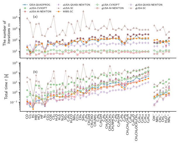
Figure 1: Benchmark testing of different ISA methods with various solvers.

IV.3 Convergence and accuracy

In this section, we first investigate the consistency and precision of entropy calculations within the LISA framework, specifically examining the effects of negative (from LISA± solvers) and non-negative (from LISA+ solvers) parameters on the entropy outcomes. For molecules with non-negative optimized $c_{a,k}$ values, the entropy differences are observed to be less than $10^{-5}$ between aLISA+ and aLISA± solvers. In cases where the pro-atom $c_{a,k}$ coefficients can take negative, aLISA± solvers are shown to achieve lower entropy values compared to aLISA+ solvers, with the difference maintained below $10^{-4}$ except for H3O+ where the difference is $-2.5\times 10^{-3}$. A detailed comparison of the converged entropy between aLISA± (represented by aLISA-M-NEWTON) and aLISA+ (represented by aLISA-SC) solvers can be found in Table 5. The entropy difference between any gLISA solvers and aLISA+ is less than $6\times 10^{-3}$.

Table 5: Comparision of converged entropy between aLISA-M-NEWTON and aLISA-SC solvers.

Molecule	aLISA-M-NEWTON	aLISA-SC	Molecule	aLISA-M-NEWTON	aLISA-SC
CO	0.06183321	0.06183321	Cl2	0.08958828	0.08975218
H2	0.02736409	0.02736409	HBr	0.07610432	0.07909211
HCl	0.03821032	0.03831474	HF	0.02978911	0.02978911
N2	0.05178624	0.05178624	CO2	0.04023066	0.04023066
COS	0.05997184	0.06003172	CS2	0.06028581	0.06037959
H2O	0.03806443	0.03806443	H2S	0.07030862	0.07042643
N2O	0.04043933	0.04043933	SO2	0.05605274	0.05604687
C2H2	0.09165923	0.09166115	H2CO	0.07787287	0.07787716
NH3	0.05774993	0.05774993	CCl4	0.12103100	0.12140725
CH4	0.04791988	0.04865526	SiH4	0.09808597	0.09813977
C2H4	0.09452415	0.09471247	CH3OH	0.08943380	0.08974105
CH3CHO	0.10559780	0.10633781	CH3NH2	0.10469464	0.10507311
C2H6	0.08808395	0.08951780	C2H5OH	0.12156226	0.12238322
C3H6	0.12559076	0.12639253	CH3OCH3	0.13892528	0.13950614
CH3COCH3	0.13185302	0.13342077	CH3NHCH3	0.14713276	0.14801049
C3H8	0.12460286	0.12648920	C3H7OH	0.15787796	0.15905492
C4H8	0.15509782	0.15773012	C6H6	0.20258266	0.20334263
CH3CH3CH3N	0.17390093	0.17510509	C4H10	0.16028960	0.16281083
C4H10O	0.19301351	0.19494893	CH3CH2OCH2CH3	0.20235187	0.20407238
C5H12	0.19608408	0.19923136	C6H14	0.23212627	0.23560304
C7H16	0.26697768	0.27137861	C8H18	0.30658548	0.31053885
OH-	0.09685251	0.09687230	NH2-	0.29375341	0.30137830
CH3+	0.21960476	0.21996092	CH3-	0.51980227	0.52591730
H3O+	0.04643185	0.04896827	NH4+	0.04948623	0.04948623

Figure 2 presents the results of the converged entropies obtained using different solvers. In general, MBIS-SC converges to the highest entropy, followed by the GISA-QUADPROG solver, while all LISA-family methods converge to the lowest entropy. Two exceptions are observed, i.e., NH2- and CH3-, where MBIS-SC has a lower entropy compared to both GISA-QUADPROG and any LISA-family solvers. This can be attributed to the lack of more diffused basis functions in GISA or LISA, because the Gaussian exponential coefficients are obtained by fitting ions with only 1 a.u. charge. By simply adding an extra Gaussian (Slater) basis function with an exponential coefficient of $0.1$ ($1.0$) for the H atom, a lower entropy can be obtained for CH3-, NH2- and OH- using aLISA-M-NEWTON or aLISA-SC as shown in Table 6.

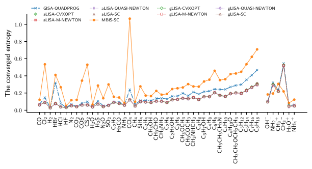
Figure 2: Converged entropy of ISA methods with various solvers.

Table 6: Converged entropy comparison between MBIS-SC and aLISA-SC (aLISA-M-NEWTON) with the addition of an extra Gaussian (Slater) basis function, each with exponential coefficients equal to $0.1$ ($1.0$). aLISA+@1g (aLISA±@1g) and aLISA+@1s (aLISA±@1s) denote aLISA-SC (aLISA-M-NEWTON) with the extra Gaussian and Slater basis functions, respectively.

Molecule	MBIS-SC	aLISA+@1g	aLISA±@1g	aLISA+@1s	aLISA±@1s
CH3-	$0.2185$	$0.1905$	$0.1752$	$0.1763$	$0.1614$
OH-	$0.1834$	$0.0479$	$0.0453$	$0.0471$	$0.0444$
NH2-	$0.1943$	$0.1098$	$0.1056$	$0.1112$	$0.1071$

Next, we compare the convergence behavior of the entropy for different ISA methods. Figure 3 displays the entropies obtained by different ISA methods at each outer iteration for four example molecules, i.e., C2H2, C2H4, C2H5OH, and C2H6. The results of other molecules can be found in the Supporting Information. To facilitate a clear comparison, we only consider the first 15 iterations for all solvers, and all iterations are included for solvers where the total number of outer iterations is less than 15, e.g., gLISA-CVXOPT and gLISA-M-NEWTON. As discussed in Ref. 79, all variants of aLISA with non-negative $c_{a,k}$ (aLISA+) or $c_{a,k}$ with both signs (aLISA±) should maintain consistency in the number of iterations, entropies, atomic charges, and $c_{a,k}$ values at each outer iteration, due to the unique solution of the strictly convex optimization problem. Therefore, we consider only the results of aLISA-SC and aLISA-M-NEWTON as specific instances representing aLISA+ and aLISA± solvers. As mathematically proven in Ref. 79, the entropy of the aLISA solvers decays monotonically. All aLISA methods converge slightly faster than GLISA-SC but generally slower than other solvers, given the initial values used in this work, as shown in Figures 1(a) and 3. Additionally, our numerical tests demonstrate that among all gLISA methods only gLISA-SC and gLISA-CVXOPT possess the characteristic of monotonically decreasing entropy. gLISA-SC exhibits slower convergence compared to all other LISA-family methods. gLISA-CVXOPT converges faster than all other LISA methods except for gLISA-M-NEWTON, but the issues of computational efficiency may impede its practical applications. The entropy of the second iteration of gLISA-M-NEWTON is higher than that of other LISA-family solvers, except for gLISA-CVXOPT, because the identity matrix is always used as the initial Hessian matrix. For gLISA-CVXOPT, the $c_{a,k}$ is optimized with respect to inequality constraints, which leads to slower entropy convergence in the first few iterations.

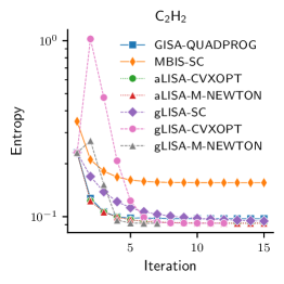
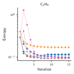
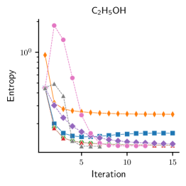
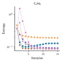
Figure 3: Evolution of the entropy of various ISA solvers.

IV.4 Comparison of AIM charges

First, we observed that all aLISA+, aLISA±, gLISA±, and gLISA+ solvers generally converge to their respective unique solutions as expected, and the corresponding AIM charges are reasonably close to each other, with the maximum charge difference being less than 0.01 a.u. However, a few exceptions include the aLISA± solvers (aLISA-M-NEWTON and aLISA-QUASI-NEWTON) for CH3-, H3O+, and NH2-, and the gLISA± (gLISA-M-NEWTON) solver for CH3- and NH2- which, compared to aLISA+, yield results that differ between 0.01 and 0.09. This suggests that allowing negative $c_{a,k}$, i.e., LISA±, could play an important role in systems of charged molecules. Additionally, there is a systematic difference in the comparison between all gLISA and aLISA methods, where CCl4 exhibits a difference of 0.02. Somewhat related, we observed a deviation between the sum of AIM charges, i.e., the molecular population, and the total number of electrons in the molecular system by all gLISA solvers. This discrepancy is attributed to the quadrature error arising from the (global) molecular grids. In principle, Eq. (39) conserves molecular charges when exact integration is applied. For simplicity and clarity, in the following analysis, we will consider AIM charges obtained by the aLISA solvers, and use aLISA-M-NEWTON and aLISA-SC solvers as representative of aLISA± and aLISA+ solvers, respectively. For simplicity, we use GISA, MBIS, aLISA±, and aLISA+ to refer to GISA-QUADPROG, MBIS-SC, aLISA-M-NEWTON, and aLISA-SC, respectively.

Figure 4 shows a series of scatter plots comparing AIM charges via the GISA, MBIS, and aLISA± methods on 48 test molecules. It should be noted that the aLISA+ are not included due to the tiny difference between aLISA± and aLISA+ in AIM charges. A consistent linear correlation exists across all elements, signifying a robust relationship between the GISA and MBIS methods respectively and the aLISA± AIM charges. This uniformity underscores the consistency in computational approaches for AIM charge determination. Most data points of MBIS for the majority of elements closely follow the diagonal line (represented as a dashed line), indicating strong methodological agreement between MBIS and aLISA±. However, a few outliers suggest possible variations in charge calculations.

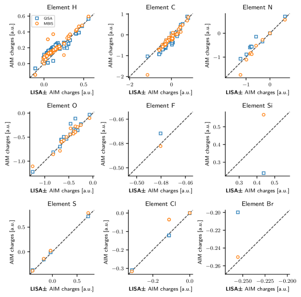
Figure 4: Comparison AIM charges among GISA, MBIS, and aLISA± for 48 molecules.

To study the deviations in AIM charges due to different methods, we compared AIM charges among the GISA, MBIS, and aLISA±, methods for CCl4, CS2, and SiH4 in the TS42 dataset and all charged molecules from the Ref. 59. The outliers in the plots are primarily attributed to these molecules. The results are listed in Table 7. Some computational values available in the literature are also listed for comparison. For the CCl4 and CS2 molecules, the electrostatic potential (ESP) fitting charges are included.Torii2003 ; Torii2004 For all charged molecules, we compiled the AIM values obtained using the Hirshfeld-E (HE) method at the UB3LYP/aug-cc-pVDZ level from Ref. 59.

Some observations can be obtained. For the CCl4 molecule, the charge comparison reveals distinct differences between the aLISA and MBIS methods. Specifically, for the carbon atom, the aLISA± (aLISA+) method estimates a charge of 0.450 (0.448), which aligns more closely with the ESP values of 0.422 (Ref. 94) and 0.380 (Ref. 95), compared to the MBIS estimate of 0.140. For the CS2 molecule, aLISA and MBIS methods yield AIM charges with opposite signs. The aLISA±/aLISA+ charge for the carbon atom is 0.073, closer to the ESP value of 0.088,Torii2003 while the MBIS method predicts a negative charge of $-0.044$. These observations suggest that, in terms of ESP fitting charges, the aLISA method provides a more accurate approximation of the atomic charges in CCl4 and CS2 compared to the MBIS method. Interestingly, the AIM charges obtained by aLISA± and aLISA+, through the addition of an extra Gaussian (Slater) basis function with exponential coefficients equal to 0.1 (1.0) for the H atom, are also listed in the table. The differences between the aLISA± and aLISA+ methods are less than 1% except for CH3- for which the differences are 7%.

Furthermore, GISA shows a trend similar to aLISA for both CCl4 and CS2 molecules. However, the AIM charges produced by GISA for CS2 are smaller than those from aLISA. Notably, for SiH4, the AIM charges from GISA are significantly lower compared to those from aLISA and MBIS.

It has been observed that MBIS can yield anomalously negative values for anionic molecules.Heidar-Zadeh2018 For all charged molecules, the aLISA results demonstrate good agreement with the HE values. In contrast, large discrepancies are evident between the MBIS and HE results for OH- and NH2-, consistent with findings from previous work.Heidar-Zadeh2018 It should be noted that the difference of AIM charges obtained by aLISA with and without extra basis functions is very small. This implies that even when aLISA converge to a higher entropy compared to MBIS, the former solvers can still predict reasonable AIM charges. The extra diffuse basis function seems to mainly contribute to the tail of the atomic density. However, this could be more important in force field development and in calculations of higher-ranking atomic moments and polarizabilities.Misquitta2014b ; Verstraelen2016

Table 7: Comparison of atomic charges among the GISA-QUADPROG (GISA), aLISA-M-NEWTON (aLISA±), aLISA-SC (aLISA+) and MBIS-SC (MBIS) methods for molecules CCl4 and CS2, along with available values from the literature. The values in the parenthesis for the aLISA±/aLISA+ solver are computed by adding an extra Gaussian and Slater basis with exponential coefficients equal to $0.1$ and $1.0$, respectively.

Molecule	Atom	GISA	aLISA±	aLISA+	MBIS	Others
CCl4	C	$0.485$	$0.450$	$0.448$	$0.140$	$0.422$ (Ref. 94) and $0.380$ (Ref. 95)
CS2	C	$0.020$	$0.073$	$0.073$	$-0.044$	$0.088$ (Ref. 94)
SiH4	Si	$0.239$	$0.443$	$0.443$	$0.568$	$--$
CH3+	C	$0.307$	$0.425$	$0.428$	$0.349$	$0.447$ (Ref. 59)
CH3-	C	$-1.032$	$-1.147$	$-1.067$	$-1.920$	$-1.047$ (Ref. 59)
			($-1.133$, $-1.146$)	($-1.039$, $-1.052$)
H3O+	O	$-0.698$	$-0.683$	$-0.693$	$-0.785$	$-0.731$ (Ref. 59)
OH-	O	$-1.223$	$-1.250$	$-1.250$	$-1.107$	$-1.200$ (Ref. 59)
			($-1.199$, $-1.205$)	($-1.181$, $-1.187$)
NH4+	N	$-0.565$	$-0.761$	$-0.761$	$-0.877$	$-0.871$ (Ref. 59)
NH2-	N	$-1.069$	$-1.183$	$-1.183$	$-1.743$	$-1.244$ (Ref. 59)
			($-1.190$, $-1.199$)	($-1.160$, $-1.173$)

V Conclusions

In this study, we conducted a comprehensive numerical analysis of various ISA solvers used in molecular density partitioning, including MBIS, GISA, and the recently developed LISA schemes. Initially, we adapted the original LISA approach to a broader framework by removing the non-negativity constraint on the pro-atomic expansion coefficients, $c_{a,k}$. This modification resulted in two sub-categories of LISA variants, termed LISA+ and LISA±, which correspond to LISA methods with and without the non-negativity requirement on $c_{a,k}$. Next, we derived an equivalent global version of LISA, denoted as gLISA, compared to the previously used two-step alternating aLISA scheme. Based on this, LISA-family methods can also be classified into two categories denoted by gLISA and aLISA with the prefix “gLISA-” and “aLISA-” to indicate the global and alternating version algorithms used, respectively. Then, by examining the critical points of the Lagrangian associated with either the global or local constrained convex optimization problem, we formulated it as a set of non-linear equations. This alternative approach provides two equivalent formulations for solving the original convex optimization problem in the form of a root-finding problem or a fixed-point problem. Therefore, alternative optimization algorithms can be employed for both aLISA and gLISA. For the root-finding problem, we used a Newton solver, while for the fixed-point problem, we utilized an iteratively self-consistent solver, along with accelerating techniques such as DIIS. Combining LISA+/LISA± and gLISA/aLISA results four different sub-categories of LISA variants, i.e., gLISA+, aLISA+, gLISA± and aLSIA±, which converge to their respective optima numerically. In the end, we developed 18 different ISA solvers, which have been implemented in the “Horton-Part” package.YingXing2023 These solvers include 1 GISA, 1 MBIS, 2 gLISA+, 2 aLISA+, 5 gLISA± and 5 aLSIA± solvers.

Regarding numerical benchmarks, we computed AIM charges for 42 organic and inorganic molecules in the TS42 database with extra 6 charged molecules from the literature using these solvers. Initially, the numerical calculations showed that two aLISA+ (aLISA-CVXOPT and aLISA-SC), two aLISA± (aLISA-M-NEWTON and aLISA-QUASI-NEWTON), two gLISA+ (gLISA-CVXOPT and gLISA-SC) and two gLISA± (gLISA-FD-DIIS and gLISA-M-NEWTON) converge for all molecules. Our numerical results show that the entropy obtained by LISA± methods is, not surprisingly, lower than that obtained with all LISA+ solvers. However, gLISA-FD-DIIS, that has no restriction on the sign of the parameters, cannot always obtain the solution with negative parameters corresponding to the lowest entropy.

The ISA solvers that have converged results were then employed to compare the performance in terms of the number of outer iterations, the total partitioning time. Additionally, we investigated the convergence behavior of entropy for these solvers. The key findings from our analysis are as follows:

1. Considering gLISA+ solvers, the gLISA-SC solver exhibited the highest number of outer iterations, making it the most computationally intensive in practice. Due to its lower number of outer iterations, the gLISA-CVXOPT solver has been observed to be more efficient for small molecules than some aLISA solvers. However, for large molecules, it remained computationally demanding due to the requirement for gradient and Hessian matrices in its optimization process.

2. For gLISA± solvers, the gLISA-M-NEWTON solver shows the best performance in terms of the number of outer iterations. However, it is computationally expensive for larger molecules due to the costly calculations of the Jacobian matrix. Using the quasi-Newton method, the gLISA-QUASI-NEWTON solver, which generally provides lower entropy at a lower computational cost, could be a potentially efficient and accurate AIM scheme. However, the numerical results show that it may not be robust for charged molecule systems but worked systematically well on the neutral molecules of our test set.

3. For all aLISA variants, tiny deviations in the outer iteration count were observed for all systems, leading to a similar total time for all aLISA methods, except for aLISA-CVXOPT where the Hessian matrix is computationally expensive.

4. After adding more diffused basis functions for CH3- and OH-, all LISA-family solvers converged to the lowest entropy levels, while the MBIS-SC solver consistently converged to the highest entropy levels. All MBIS, gLISA+, and aLISA solvers showed a monotonic decay of the entropy. However, the GISA-QUADPROG solver exhibits non-monotonic entropy convergence with respect to the outer iteration count, which is in alignment with previous studies. The MBIS-SC solver emerged as the fastest among the tested solvers except for some gLISA solvers, e.g., gLISA-QUASI-NEWTON but suffers from higher entropy values.

Next, we compared the AIM charges obtained by the MBIS, GISA, and LISA-family methods. We found that the difference in AIM charges obtained by different LISA-family solvers was tiny except for some charged molecules. Therefore, we chose aLISA-M-NEWTON and aLISA-SC as the representative of all aLISA± and aLISA+ solvers. The results suggest that all aLISA± and aLISA+, i.e., aLISA, solvers provide more accurate results than MBIS compared to ESP charges. In addition, LISA solvers also show better performance in charged molecular systems compared to the MBIS method regarding the AIM charges of anionic molecules.

In conclusion, this study offers a comprehensive evaluation of the performance of various ISA methods employing different solvers. We have implemented more computationally robust and efficient LISA-family variants, and our numerical results demonstrate that some of them even provide lower information entropy compared to MBIS, with lower computational costs. Table 8 presents, reviews, and assesses different ISA methods based on the criteria presented in Ref. 59, with a recommended solver for each LISA category.

Table 8: Checklist of desired AIM traits for different ISA methods.

			LISA
			LISA+		LISA±
Features	GISA	MBIS	gLISA+	aLISA+	gLISA±	aLISA±
Mathematical
Universality	✓	✓	✓	✓	✓	✓
Information-Theoretic	✓	✓	✓	✓	✓	✓
Variational $\rho(r)$	×	✓	✓	✓	✓	✓
Variational $\rho^{0}_{a}(r)$	×	✓	✓	✓	✓	✓
Uniqueness	×	×	✓	✓	✓	✓
Black box (Bias-FreeHeidar-Zadeh2018 )	✓	✓	✓	✓	✓	✓
Practical
Computational Robustness	×	?	✓	✓	?	✓
Computational Efficiency	✓	✓	✓	✓	✓	✓

• ✓ indicates the method complies with the feature.

• × indicates the method does not comply with the feature.

• ? indicates that further investigation is required.

• Recommended gLISA+ solver: gLISA-CVXOPT.

• Recommended gLISA± solver: gLISA-M-NEWTON.

• Recommended aLISA+ solver: aLISA-SC.

• Recommended aLISA± solver: aLISA-M-NEWTON.

It is important to note that the chemical accuracy and robustness of LISA-family methods have not been explored in this work. These aspects are vital for practical applications and will be the focus of future studies. This study, therefore, establishes a numerical groundwork for future research on LISA partitioning schemes in molecular density partitioning.

Dataset Availability Statement

The data that support the findings of this study are available within the article and its supplementary material. The “Horton-Part” package can be found at https://github.com/LISA-partitioning-method/horton-part.

Supplementary Material

The Supplementary Material is a PDF document that includes the exponents and initial values for the Gaussian density basis used in both GISA and LISA methods, and the evolution of entropy for other molecules, which are not covered in the main text.

References

- (1) David A. Case, Thomas E. Cheatham III, Tom Darden, Holger Gohlke, Ray Luo, Kenneth M. Merz Jr., Alexey Onufriev, Carlos Simmerling, Bing Wang, and Robert J. Woods. The Amber biomolecular simulation programs. J. Comput. Chem., 26(16):1668–1688, 2005.
- (2) Romelia Salomon-Ferrer, David A. Case, and Ross C. Walker. An overview of the Amber biomolecular simulation package. WIREs Comput. Mol. Sci., 3(2):198–210, 2013.
- (3) Romelia Salomon-Ferrer, Andreas W. Götz, Duncan Poole, Scott Le Grand, and Ross C. Walker. Routine Microsecond Molecular Dynamics Simulations with AMBER on GPUs. 2. Explicit Solvent Particle Mesh Ewald. J. Chem. Theory Comput., 9(9):3878–3888, 2013.
- (4) Bernard R. Brooks, Robert E. Bruccoleri, Barry D. Olafson, David J. States, S. Swaminathan, and Martin Karplus. CHARMM: A program for macromolecular energy, minimization, and dynamics calculations. J. Comput. Chem., 4(2):187–217, 1983.
- (5) B. R. Brooks, C. L. Brooks III, A. D. Mackerell Jr., L. Nilsson, R. J. Petrella, B. Roux, Y. Won, G. Archontis, C. Bartels, S. Boresch, A. Caflisch, L. Caves, Q. Cui, A. R. Dinner, M. Feig, S. Fischer, J. Gao, M. Hodoscek, W. Im, K. Kuczera, T. Lazaridis, J. Ma, V. Ovchinnikov, E. Paci, R. W. Pastor, C. B. Post, J. Z. Pu, M. Schaefer, B. Tidor, R. M. Venable, H. L. Woodcock, X. Wu, W. Yang, D. M. York, and M. Karplus. CHARMM: The biomolecular simulation program. J. Comput. Chem., 30(10):1545–1614, 2009.
- (6) Sandeep Patel, Alexander D. Mackerell Jr., and Charles L. Brooks III. CHARMM fluctuating charge force field for proteins: II Protein/solvent properties from molecular dynamics simulations using a nonadditive electrostatic model. J. Comput. Chem., 25(12):1504–1514, 2004.
- (7) Sandeep Patel and Charles L. Brooks III. CHARMM fluctuating charge force field for proteins: I parameterization and application to bulk organic liquid simulations. J. Comput. Chem., 25(1):1–16, 2004.
- (8) K. Vanommeslaeghe and A. D. MacKerell. CHARMM additive and polarizable force fields for biophysics and computer-aided drug design. Biochim. Biophys. Acta (BBA) - Gen. Subj., 1850(5):861–871, 2015.
- (9) Xiao Zhu, Pedro E. M. Lopes, and Alexander D. MacKerell Jr. Recent developments and applications of the CHARMM force fields. WIREs Comput. Mol. Sci., 2(1):167–185, 2012.
- (10) Edward Harder, Wolfgang Damm, Jon Maple, Chuanjie Wu, Mark Reboul, Jin Yu Xiang, Lingle Wang, Dmitry Lupyan, Markus K. Dahlgren, Jennifer L. Knight, Joseph W. Kaus, David S. Cerutti, Goran Krilov, William L. Jorgensen, Robert Abel, and Richard A. Friesner. OPLS3: A Force Field Providing Broad Coverage of Drug-like Small Molecules and Proteins. J. Chem. Theory Comput., 12(1):281–296, 2016.
- (11) William L. Jorgensen, David S. Maxwell, and Julian Tirado-Rives. Development and Testing of the OPLS All-Atom Force Field on Conformational Energetics and Properties of Organic Liquids. J. Am. Chem. Soc., 118(45):11225–11236, 1996.
- (12) H. J. C. Berendsen, D. van der Spoel, and R. van Drunen. GROMACS: A message-passing parallel molecular dynamics implementation. Comput. Phys. Commun., 91(1):43–56, 1995.
- (13) Sander Pronk, Szilárd Páll, Roland Schulz, Per Larsson, Pär Bjelkmar, Rossen Apostolov, Michael R. Shirts, Jeremy C. Smith, Peter M. Kasson, David van der Spoel, Berk Hess, and Erik Lindahl. GROMACS 4.5: A high-throughput and highly parallel open source molecular simulation toolkit. Bioinformatics, 29(7):845–854, 2013.
- (14) David Van Der Spoel, Erik Lindahl, Berk Hess, Gerrit Groenhof, Alan E. Mark, and Herman J. C. Berendsen. GROMACS: Fast, flexible, and free. J. Comput. Chem., 26(16):1701–1718, 2005.
- (15) James C. Phillips, Rosemary Braun, Wei Wang, James Gumbart, Emad Tajkhorshid, Elizabeth Villa, Christophe Chipot, Robert D. Skeel, Laxmikant Kalé, and Klaus Schulten. Scalable molecular dynamics with NAMD. J. Comput. Chem., 26(16):1781–1802, 2005.
- (16) S. Scott Zimmerman, Marcia S. Pottle, George Némethy, and Harold A. Scheraga. Conformational Analysis of the 20 Naturally Occurring Amino Acid Residues Using ECEPP. Macromolecules, 10(1):1–9, 1977.
- (17) Jay W. Ponder, Chuanjie Wu, Pengyu Ren, Vijay S. Pande, John D. Chodera, Michael J. Schnieders, Imran Haque, David L. Mobley, Daniel S. Lambrecht, Robert A. Distasio, Martin Head-Gordon, Gary N.I. Clark, Margaret E. Johnson, and Teresa Head-Gordon. Current status of the AMOEBA polarizable force field. J. Phys. Chem. B, 114(8):2549–2564, 2010.
- (18) Norman L. Allinger, Young H. Yuh, and Jenn Huei Lii. Molecular mechanics. The MM3 force field for hydrocarbons. 1. J. Am. Chem. Soc., 111(23):8551–8566, 1989.
- (19) Norman L. Allinger, Kuo-Hsiang Chen, Jenn-Huei Lii, and Kathleen A. Durkin. Alcohols, ethers, carbohydrates, and related compounds. I. The MM4 force field for simple compounds. J. Comput. Chem., 24(12):1447–1472, 2003.
- (20) Thomas A. Halgren. Merck molecular force field. I. Basis, form, scope, parameterization, and performance of MMFF94. J. Comput. Chem., 17(5-6):490–519, 1996.
- (21) Thomas A. Halgren. MMFF VII. Characterization of MMFF94, MMFF94s, and other widely available force fields for conformational energies and for intermolecular-interaction energies and geometries. J. Comput. Chem., 20(7):730–748, 1999.
- (22) A. T. Hagler and C. S. Ewig. On the use of quantum energy surfaces in the derivation of molecular force fields. Comput. Phys. Commun., 84(1):131–155, 1994.
- (23) M. J. Hwang, T. P. Stockfisch, and A. T. Hagler. Derivation of Class II Force Fields. 2. Derivation and Characterization of a Class II Force Field, CFF93, for the Alkyl Functional Group and Alkane Molecules. J. Am. Chem. Soc., 116(6):2515–2525, 1994.
- (24) M.-J. Hwang, X. Ni, M. Waldman, C. S. Ewig, and A. T. Hagler. Derivation of class II force fields. VI. Carbohydrate compounds and anomeric effects. Biopolymers, 45(6):435–468, 1998.
- (25) J.r. Maple, M.-J. Hwang, T.p. Stockfisch, and A.t. Hagler. Derivation of Class II Force Fields. III. Characterization of a Quantum Force Field for Alkanes. Isr. J. Chem., 34(2):195–231, 1994.
- (26) J. R. Maple, M.-J. Hwang, T. P. Stockfisch, U. Dinur, M. Waldman, C. S. Ewig, and A. T. Hagler. Derivation of class II force fields. I. Methodology and quantum force field for the alkyl functional group and alkane molecules. J. Comput. Chem., 15(2):162–182, 1994.
- (27) J. R. Maple, M.-J. Hwang, K. J. Jalkanen, T. P. Stockfisch, and A. T. Hagler. Derivation of class II force fields: V. Quantum force field for amides, peptides, and related compounds. J. Comput. Chem., 19(4):430–458, 1998.
- (28) C. J. Casewit, K. S. Colwell, and A. K. Rappe. Application of a universal force field to organic molecules. J. Am. Chem. Soc., 114(25):10035–10046, 1992.
- (29) A. K. Rappe, C. J. Casewit, K. S. Colwell, W. A. III Goddard, and W. M. Skiff. UFF, a full periodic table force field for molecular mechanics and molecular dynamics simulations. J. Am. Chem. Soc., 114(25):10024–10035, 1992.
- (30) S. Lifson and A. Warshel. Consistent Force Field for Calculations of Conformations, Vibrational Spectra, and Enthalpies of Cycloalkane and n-Alkane Molecules. J. Chem. Phys., 49(11):5116–5129, 1968.
- (31) Arieh Warshel and Shneior Lifson. Consistent Force Field Calculations. II. Crystal Structures, Sublimation Energies, Molecular and Lattice Vibrations, Molecular Conformations, and Enthalpies of Alkanes. J. Chem. Phys., 53(2):582–594, 1970.
- (32) Arnold T. Hagler, Peter S. Stern, Shneior Lifson, and Sara Ariel. Urey-Bradley force field, valence force field, and ab initio study of intramolecular forces in tri-tert-butylmethane and isobutane. J. Am. Chem. Soc., 101(4):813–819, 1979.
- (33) A. Warshel and M. Levitt. Theoretical studies of enzymic reactions: Dielectric, electrostatic and steric stabilization of the carbonium ion in the reaction of lysozyme. J. Mol. Biol., 103(2):227–249, 1976.
- (34) George A. Kaminski, Harry A. Stern, B. J. Berne, Richard A. Friesner, Yixiang X. Cao, Robert B. Murphy, Ruhong Zhou, and Thomas A. Halgren. Development of a polarizable force field for proteins via ab initio quantum chemistry: First generation model and gas phase tests. J. Comput. Chem., 23(16):1515–1531, 2002.
- (35) Pengyu Ren and Jay W. Ponder. Consistent treatment of inter- and intramolecular polarization in molecular mechanics calculations. J. Comput. Chem., 23(16):1497–1506, 2002.
- (36) William L. Jorgensen, Kasper P. Jensen, and Anastassia N. Alexandrova. Polarization Effects for Hydrogen-Bonded Complexes of Substituted Phenols with Water and Chloride Ion. J. Chem. Theory Comput., 3(6):1987–1992, 2007.
- (37) Yue Shi, Zhen Xia, Jiajing Zhang, Robert Best, Chuanjie Wu, Jay W. Ponder, and Pengyu Ren. Polarizable Atomic Multipole-Based AMOEBA Force Field for Proteins. J. Chem. Theory Comput., 9(9):4046–4063, 2013.
- (38) Guillaume Lamoureux and Benoît Roux. Modeling induced polarization with classical Drude oscillators: Theory and molecular dynamics simulation algorithm. J. Chem. Phys., 119(6):3025–3039, 2003.
- (39) Haibo Yu, Tomas Hansson, and Wilfred F. van Gunsteren. Development of a simple, self-consistent polarizable model for liquid water. J. Chem. Phys., 118(1):221–234, 2003.
- (40) Justin A. Lemkul, Jing Huang, Benoît Roux, and Alexander D. Jr. MacKerell. An Empirical Polarizable Force Field Based on the Classical Drude Oscillator Model: Development History and Recent Applications. Chem. Rev., 116(9):4983–5013, 2016.
- (41) Anna-Pitschna E. Kunz and Wilfred F. van Gunsteren. Development of a Nonlinear Classical Polarization Model for Liquid Water and Aqueous Solutions: COS/D. J. Phys. Chem. A, 113(43):11570–11579, 2009.
- (42) Wilfried J. Mortier, Karin Van Genechten, and Johann Gasteiger. Electronegativity equalization: Application and parametrization. J. Am. Chem. Soc., 107(4):829–835, 1985.
- (43) Wilfried J. Mortier, Swapan K. Ghosh, and S. Shankar. Electronegativity-equalization method for the calculation of atomic charges in molecules. J. Am. Chem. Soc., 108(15):4315–4320, 1986.
- (44) Seyit Kale and Judith Herzfeld. Pairwise Long-Range Compensation for Strongly Ionic Systems. J. Chem. Theory Comput., 7(11):3620–3624, 2011.
- (45) Seyit Kale, Judith Herzfeld, Stacy Dai, and Michael Blank. Lewis-inspired representation of dissociable water in clusters and Grotthuss chains. J. Biol. Phys., 38(1):49–59, 2012.
- (46) Seyit Kale and Judith Herzfeld. Natural polarizability and flexibility via explicit valency: The case of water. J. Chem. Phys., 136(8):084109, 2012.
- (47) Chen Bai, Seyit Kale, and Judith Herzfeld. Chemistry with semi-classical electrons: Reaction trajectories auto-generated by sub-atomistic force fields. Chem. Sci., 8(6):4203–4210, 2017.
- (48) Maarten Cools-Ceuppens, Joni Dambre, and Toon Verstraelen. Modeling Electronic Response Properties with an Explicit-Electron Machine Learning Potential. J. Chem. Theory Comput., 18(3):1672–1691, 2022.
- (49) T. Verstraelen, P. W. Ayers, V. Van Speybroeck, and M. Waroquier. ACKS2: Atom-condensed Kohn-Sham DFT approximated to second order. J. Chem. Phys., 138(7):074108, 2013.
- (50) Toon Verstraelen, Steven Vandenbrande, and Paul W. Ayers. Direct computation of parameters for accurate polarizable force fields. J. Chem. Phys., 141(19):194114, 2014.
- (51) YingXing Cheng and Toon Verstraelen. A new framework for frequency-dependent polarizable force fields. J. Chem. Phys., 157(12):124106, 2022.
- (52) Alston J. Misquitta and Anthony J. Stone. ISA-pol: distributed polarizabilities and dispersion models from a basis-space implementation of the iterated stockholder atoms procedure. Theor. Chem. Acc., 137(11):153, 2018.
- (53) John F. Dobson, Angela White, and Angel Rubio. Asymptotics of the Dispersion Interaction: Analytic Benchmarks for van der Waals Energy Functionals. Phys. Rev. Lett., 96(7):073201, 2006.
- (54) John F. Dobson and Tim Gould. Calculation of dispersion energies. J. Phys. Condens. Matter, 24(7):073201, 2012.
- (55) Alston J. Misquitta, James Spencer, Anthony J. Stone, and Ali Alavi. Dispersion interactions between semiconducting wires. Phys. Rev. B, 82(7):075312, 2010.
- (56) Alston J. Misquitta, Ryo Maezono, Neil D. Drummond, Anthony J. Stone, and Richard J. Needs. Anomalous nonadditive dispersion interactions in systems of three one-dimensional wires. Phys. Rev. B, 89(4):045140, 2014.
- (57) John F. Dobson, Andreas Savin, János G. Ángyán, and Ru-Fen Liu. Spooky correlations and unusual van der waals forces between gapless and near-gapless molecules. J. Chem. Phys., 145(20):204107, 2016.
- (58) YingXing Cheng and Toon Verstraelen. The significance of fluctuating charges for molecular polarizability and dispersion coefficients. J. Chem. Phys., 159(9):094111, 2023.
- (59) Farnaz Heidar-Zadeh, Paul W. Ayers, Toon Verstraelen, Ivan Vinogradov, Esteban Vöhringer-Martinez, and Patrick Bultinck. Information-Theoretic Approaches to Atoms-in-Molecules: Hirshfeld Family of Partitioning Schemes. J. Phys. Chem. A, 122(17):4219–4245, 2018.
- (60) R. S. Mulliken. Electronic Population Analysis on LCAO–MO Molecular Wave Functions. I. J. Chem. Phys., 23(10):1833–1840, 1955.
- (61) R. S. Mulliken. Electronic Population Analysis on LCAO-MO Molecular Wave Functions. III. Effects of Hybridization on Overlap and Gross AO Populations. J. Chem. Phys., 23(12):2338–2342, 1955.
- (62) R. S. Mulliken. Electronic Population Analysis on LCAO-MO Molecular Wave Functions. IV. Bonding and Antibonding in LCAO and Valence-Bond Theories. J. Chem. Phys., 23(12):2343–2346, 1955.
- (63) R. S. Mulliken. Electronic Population Analysis on LCAO–MO Molecular Wave Functions. II. Overlap Populations, Bond Orders, and Covalent Bond Energies. J. Chem. Phys., 23(10):1841–1846, 1955.
- (64) Per-Olov Löwdin. On the Non-Orthogonality Problem Connected with the Use of Atomic Wave Functions in the Theory of Molecules and Crystals. J. Chem. Phys., 18(3):365–375, 1950.
- (65) Per-Olov Löwdin. On the Nonorthogonality Problem*. In Per-Olov Löwdin, editor, Advances in Quantum Chemistry, pages 185–199. Academic Press, January 1970.
- (66) Ernest R. Davidson. Electronic Population Analysis of Molecular Wavefunctions. J. Chem. Phys., 46(9):3320–3324, 1967.
- (67) F. L. Hirshfeld. Bonded-atom fragments for describing molecular charge densities. Theoret. Chim. Acta, 44(2):129–138, 1977.
- (68) Patrick Bultinck, Christian Van Alsenoy, Paul W. Ayers, and Ramon Carbó-Dorca. Critical analysis and extension of the Hirshfeld atoms in molecules. J. Chem. Phys., 126(14):144111, 2007.
- (69) R. F. W. Bader and P. M. Beddall. Virial Field Relationship for Molecular Charge Distributions and the Spatial Partitioning of Molecular Properties. J. Chem. Phys., 56(7):3320–3329, 1972.
- (70) Paul W. Ayers. Atoms in molecules, an axiomatic approach. I. Maximum transferability. J. Chem. Phys., 113(24):10886–10898, 2000.
- (71) Timothy C. Lillestolen and Richard J. Wheatley. Redefining the atom: atomic charge densities produced by an iterative stockholder approach. Chem. Commun., 0(45):5909–5911, 2008.
- (72) Timothy C. Lillestolen and Richard J. Wheatley. Atomic charge densities generated using an iterative stockholder procedure. J. Chem. Phys., 131(14):144101, 2009.
- (73) Patrick Bultinck, David L. Cooper, and Dimitri Van Neck. Comparison of the Hirshfeld-I and iterated stockholder atoms in molecules schemes. Phys. Chem. Chem. Phys., 11(18):3424–3429, 2009.
- (74) T. Verstraelen, P. W. Ayers, V. Van Speybroeck, and M. Waroquier. The conformational sensitivity of iterative stockholder partitioning schemes. Chem. Phys. Lett., 545:138–143, 2012.
- (75) T. Verstraelen, P. W. Ayers, V. Van Speybroeck, and M. Waroquier. Hirshfeld-E Partitioning: AIM Charges with an Improved Trade-off between Robustness and Accurate Electrostatics. J. Chem. Theory Comput., 9(5):2221–2225, 2013.
- (76) Alston J. Misquitta, Anthony J. Stone, and Farhang Fazeli. Distributed Multipoles from a Robust Basis-Space Implementation of the Iterated Stockholder Atoms Procedure. J. Chem. Theory Comput., 10(12):5405–5418, 2014.
- (77) Farnaz Heidar-Zadeh and Paul W. Ayers. How pervasive is the Hirshfeld partitioning? J. Chem. Phys., 142(4):044107, 2015.
- (78) Toon Verstraelen, Steven Vandenbrande, Farnaz Heidar-Zadeh, Louis Vanduyfhuys, Veronique Van Speybroeck, Michel Waroquier, and Paul W. Ayers. Minimal Basis Iterative Stockholder: Atoms in Molecules for Force-Field Development. J. Chem. Theory Comput., 12(8):3894–3912, 2016.
- (79) Robert Benda, Eric Cancès, Virginie Ehrlacher, and Benjamin Stamm. Multi-center decomposition of molecular densities: A mathematical perspective. J. Chem. Phys., 156(16):164107, 2022.
- (80) T. C. Lillestolen and R. J. Wheatley. First-Principles Calculation of Local Atomic Polarizabilities. J. Phys. Chem. A, 111(43):11141–11146, 2007.
- (81) Robert G. Parr, Paul W. Ayers, and Roman F. Nalewajski. What Is an Atom in a Molecule? J. Phys. Chem. A, 109(17):3957–3959, 2005.
- (82) Harel Weinstein, Peter Politzer, and Shalom Srebrenik. A misconception concerning the electronic density distribution of an atom. Theor. chim. acta, 38(2):159–163, 1975.
- (83) Alfred M. Simas, Robin P. Sagar, Andrew C. T. Ku, and Vedene H. Smith Jr. The radial charge distribution and the shell structure of atoms and ions. Can. J. Chem., 66(8):1923–1930, 1988.
- (84) Paul W. Ayers and Robert G. Parr. Sufficient condition for monotonic electron density decay in many-electron systems. Int. J. Quantum Chem., 95(6):877–881, 2003.
- (85) A. J. Stone. Distributed multipole analysis, or how to describe a molecular charge distribution. Chem. Phys. Lett., 83(2):233–239, 1981.
- (86) Maxime Chupin, Mi-Song Dupuy, Guillaume Legendre, and Éric Séré. Convergence analysis of adaptive DIIS algorithms with application to electronic ground state calculations. ESAIM: Math. Model. Numer. Anal., 55(6):2785–2825, 2021.
- (87) A. D. Becke. A multicenter numerical integration scheme for polyatomic molecules. J. Chem. Phys., 88(4):2547–2553, 1988.
- (88) Stéphane Caron, Daniel Arnström, Suraj Bonagiri, Antoine Dechaume, Nikolai Flowers, Adam Heins, Takuma Ishikawa, Dustin Kenefake, Giacomo Mazzamuto, Donato Meoli, Brendan O’Donoghue, Adam A. Oppenheimer, Abhishek Pandala, Juan José Quiroz Omaña, Nikitas Rontsis, Paarth Shah, Samuel St-Jean, Nicola Vitucci, Soeren Wolfers, @bdelhaisse, @MeindertHH, @rimaddo, @urob, and @shaoanlu. qpsolvers: Quadratic Programming Solvers in Python, 2023. Accessed on Jan 16, 2024.
- (89) Martin Andersen, Joachim Dahl, and Lieven Vandenberghe. Cvxopt, 2023. Accessed on Sep 15, 2023.
- (90) YingXing Cheng. Horton-part 1.1.3, 2024. Accessed on Apr 08, 2024.
- (91) M. J. Frisch, G. W. Trucks, H. B. Schlegel, G. E. Scuseria, M. A. Robb, J. R. Cheeseman, G. Scalmani, V. Barone, G. A. Petersson, H. Nakatsuji, X. Li, M. Caricato, A. V. Marenich, J. Bloino, B. G. Janesko, R. Gomperts, B. Mennucci, H. P. Hratchian, J. V. Ortiz, A. F. Izmaylov, J. L. Sonnenberg, D. Williams-Young, F. Ding, F. Lipparini, F. Egidi, J. Goings, B. Peng, A. Petrone, T. Henderson, D. Ranasinghe, V. G. Zakrzewski, J. Gao, N. Rega, G. Zheng, W. Liang, M. Hada, M. Ehara, K. Toyota, R. Fukuda, J. Hasegawa, M. Ishida, T. Nakajima, Y. Honda, O. Kitao, H. Nakai, T. Vreven, K. Throssell, J. A. Montgomery, Jr., J. E. Peralta, F. Ogliaro, M. J. Bearpark, J. J. Heyd, E. N. Brothers, K. N. Kudin, V. N. Staroverov, T. A. Keith, R. Kobayashi, J. Normand, K. Raghavachari, A. P. Rendell, J. C. Burant, S. S. Iyengar, J. Tomasi, M. Cossi, J. M. Millam, M. Klene, C. Adamo, R. Cammi, J. W. Ochterski, R. L. Martin, K. Morokuma, O. Farkas, J. B. Foresman, and D. J. Fox. Gaussian˜16 Revision C.01, 2016. Gaussian Inc. Wallingford CT.
- (92) W. Kohn and L. J. Sham. Self-Consistent Equations Including Exchange and Correlation Effects. Phys. Rev., 140(4A):A1133–A1138, 1965.
- (93) Rick A. Kendall, Thom H. Dunning, and Robert J. Harrison. Electron affinities of the first-row atoms revisited. systematic basis sets and wave functions. J. Chem. Phys., 96(9):6796–6806, 1992.
- (94) Hajime Torii. The role of atomic quadrupoles in intermolecular electrostatic interactions of polar and nonpolar molecules. J. Chem. Phys., 119(4):2192–2198, 2003.
- (95) Hajime Torii. Atomic quadrupolar effect in the methanol–CCl4 and water–CCl4 intermolecular interactions. Chem. Phys. Lett., 393(1):153–158, 2004.