Effective Front-Descent Algorithms with Convergence Guarantees

Abstract

In this manuscript, we address continuous unconstrained optimization problems and we discuss descent type methods for the reconstruction of the Pareto set. Specifically, we analyze the class of Front Descent methods, which generalizes the Front Steepest Descent algorithm allowing the employment of suitable, effective search directions (e.g., Newton, Quasi-Newton, Barzilai-Borwein). We provide a deep characterization of the behavior and the mechanisms of the algorithmic framework, and we prove that, under reasonable assumptions, standard convergence results and some complexity bounds hold for the generalized approach. Moreover, we prove that popular search directions can indeed be soundly used within the framework. Then, we provide a completely novel type of convergence results, concerning the sequence of sets produced by the procedure. In particular, iterate sets are shown to asymptotically approach stationarity for all of their points; additionally, in finite precision settings, the sets are shown to only be enriched through exploration steps in later iterations, and suitable stopping conditions can be devised. Finally, the results from a large experimental benchmark show that the proposed class of approaches far outperforms state-of-the-art methodologies.

90C29, 90C26, 90C30

1 Introduction

In this paper, we are interested in multi-objective optimization problems of the form

(1) $$\min_{x\in\mathbb{R}^{n}}\;F(x)=(f_{1}(x),\ldots,f_{m}(x))^{\top},$$

where $F:\mathbb{R}^{n}\to\mathbb{R}^{m}$ is a continuously differentiable function. Plenty of real-world problems can be formalized as instances of this mathematical framework, see, e.g., [12, 15, 21, 28]; basically, this is the case of all tasks where the quality of a solution is measured based on more than a single criterion - i.e., many objective functions. Clearly, a solution which is simultaneously optimal for each individual objective function is unlikely to exist. For this reason, Pareto’s theory is commonly brought into play to characterize the concept of optimality in this class of problems. For a thorough discussion on continuous multi-objective optimization, we refer the reader to [7].

Pareto optimal solutions provide, in rough terms, unimprovable trade-offs among the objectives. The set of all Pareto optimal solutions is called the Pareto set of the problem, and the image of this set through $F$ is referred to as Pareto front. In applications, it is often preferable to leave to a knowledgeable decision maker the choice of the most suitable among the optimal trade-offs. In this perspective, we can understand the increasing interest towards algorithms capable of generating (a uniform and spread approximation of) the full Pareto front of multi-objective problems.

Standard approaches to tackle problems of the form Eq. 1 include scalarization and evolutionary algorithms [5]. However, both classes of methods have shortcomings: evolutionary algorithms, although flexible, have no theoretical guarantees and poor scalability [20, Sec. 4.2]; on the other hand, scalarization requires a careful choice of the weights [8, Sec. 7], and without suitable regularity assumptions large parts of the front are often even unobtainable [7, Sec. 4.1].

A more recent family of approaches thus started drawing interest: descent methods. Inspired by the seminal work of Fliege and Svaiter [9], extensions of classical descent algorithms for single-objective optimization started being proposed [8, 11, 19, 23, 27]. Initially, these algorithms were designed to produce a single efficient solution of the problem; steepest-descent type methodologies could therefore be employed to refine given solutions [20], or used in a multi-start fashion to produce Pareto front approximations. However, multi-starting single point algorithms does not allow in general to generate spread and uniform fronts. To overcome this limitation, in recent years descent methods have been proposed that explicitly handle a list of candidate solutions: the set of points is improved in a structured way, as a whole, at each iteration [3, 4, 18, 22, 25].

In this work, we are mainly focused on the Front Steepest Descent (FSD) method, originally proposed in [3] and refined in [18]. The algorithm works carrying out, from each point in the current set of solutions, line searches along directions that are of descent for all or for a subset of objectives. This strategy ensures not only to improve the solutions, driving them towards the stationarity, but also to move towards unexplored regions of the Pareto front.

The present work has multiple aims: first, we provide an improved theoretical characterization of the mechanisms of FSD methods and, in particular, of the produced sequences of solutions. The new theoretical perspective opens up the use, within the algorithm, of other types of descent directions that have widely be shown to be effective in the single-point setting (for instance, the class of Newton-type directions is particularly appealing [8, 11, 19, 27]).

The discussion therefore shift towards a broader class of algorithms than simple FSD, which we call Front Descent (FD) methods. This family of algorithms is deeply analyzed from the theoretical point of view: on the one hand, a simple condition on search directions allows to recover the same global convergence guarantees known in the literature for base FSD; moreover, some complexity bound is provided and, for specific choices of directions, we can also prove faster local convergence rates for some sequences of solutions.

On the other hand, under an additional, reasonable assumption on algorithm’s implementation, we are able to obtain convergence properties related to any sequence of solutions and, most importantly, to the entire set of points iteratively updated by the procedure. This type of results, novel in the literature, allows us

• to provide a theoretical characterization of empirically observed behaviors of FD algorithms;

• to properly define suitable stopping conditions.

Finally, thorough numerical experiments show that the proposed methods can exhibit significantly superior performance than base FSD and other state-of-the-art methods for Pareto front reconstruction in continuous optimization.

The rest of the paper is organized as follows. In Section 2, we review the preliminary material needed to read the work; in particular, we recall the basic concepts of multi-objective optimization in Section 2.1, the front steepest descent algorithm in Section 2.2 and popular search directions for multi-objective optimization in Section 2.3. Then, we provide a discussion on linked sequences produced by FSD in Section 3. In Section 4, we describe the main algorithmic framework proposed in this work. Then, we provide a thorough theoretical analysis of the methodology in Section 5: in Section 5.1 we give results concerning linked sequences produced by the algorithm, whereas in Section 5.2 we carry out the novel analysis concerning the sequence of sets of solutions. Next, in Section 6, we show the results of the computational experiments assessing the effectiveness of the proposed class of methods. We finally give some concluding remarks in Section 7.

2 Preliminaries

In the next subsections, we provide brief overviews on basic concepts in multi-objective optimization, the front steepest descent method and descent directions.

2.1 Basic concepts in multi-objective optimization

Descent algorithms in multi-objective optimization (MOO) are designed to solve instances of problem Eq. 1 according to the concepts of Pareto optimality. It is therefore useful to begin the discussion recalling some key definitions; first of all, we employ the standard partial ordering on $\mathbb{R}^{m}$: $u\leq v$ means $u_{i}\leq v_{i}$ for all $i=1,\ldots,m$; similarly, $u<v$ if $u_{i}<v_{i}$ for all $i$; moreover we denote by $u\lneqq v$ when $u\leq v$ and $u\neq v$. This third relation allows to introduce the notion of dominance between solutions of Eq. 1: given $x,y\in\mathbb{R}^{n}$, we say that $y$ is dominated by $x$ if $F(x)\lneqq F(y)$.

It is now possible to introduce the formal definitions of Pareto optimality.

Definition 2.1.

A point $\bar{x}\in\mathbb{R}^{n}$ is called

1. Pareto optimal (or efficient) for problem Eq. 1 if $\nexists\;y\in\mathbb{R}^{n}$ s.t. $F(y)\lneqq F(\bar{x})$, i.e., $y$ dominates $\bar{x}$;

2. weakly Pareto optimal for problem Eq. 1 if $\nexists\;y\in\mathbb{R}^{n}$ s.t. $F(y)<F(\bar{x})$.

Clearly, Pareto optimality, which is a quite strong condition, implies weak Pareto optimality. Note that local versions of the above optimality concepts can also be given; in that case, the property has to hold in a neighborhood of $\bar{x}$. Under differentiability assumptions, a necessary condition for weak efficiency is Pareto-stationarity.

Lemma 2.2.

Let $F:\mathbb{R}^{n}\to\mathbb{R}^{m}$ be a continuously differentiable function and $\bar{x}$ be a (local) weakly Pareto optimal point for problem Eq. 1. Then, $\bar{x}$ is Pareto-stationary for problem Eq. 1, i.e., $\min\limits_{d\in\mathbb{R}^{n}}\max\limits_{j=1,\ldots,m}\nabla f_{j}(\bar{x})^{\top}d=0.$

The three conditions - Pareto optimality, weak Pareto optimality and Pareto stationarity - become equivalent under strict convexity assumptions on $F$ [8].

Taking inspiration from traditional nonlinear programming, a key tool exploited to characterize continuous MOO problems and to define algorithms is that of (multi-objective) descent direction.

Definition 2.3.

Let $x\in\mathbb{R}^{n}$. A direction $d\in\mathbb{R}^{n}$ is referred to as a

• common descent direction at $x$ if, for all $j=1,\ldots,m$, $d$ is a descent direction for $f_{j}$ at $x$.

• partial descent direction at $x$ if there exists $I\subset\{1,\ldots,m\}$ such that, for all $j\in I$, $d$ is a descent direction for $f_{j}$ at $x$.

Lemma 2.4.

Let $x\in\mathbb{R}^{n}$ and $d\in\mathbb{R}^{n}$.

1. If $\max\limits_{j=1,\ldots,m}\nabla f_{j}(x)^{\top}d<0,$ then $d$ is a common descent direction for $F$ at $x$.

2. If there exists $I\subset\{1,\ldots,m\}$ such that $\max\limits_{j\in I}\nabla f_{j}(x)^{\top}d<0$, then $d$ is a partial descent direction for $F$ at $x$.

If we denote by $J_{F}(x)$ the Jacobian of $F$, the above conditions can be rewritten in a compact way as $J_{F}(x)d<0$ and $(J_{F}(x)d)_{I}<0$, respectively. We can also denote by $\mathcal{D}(x,d)$ the quantity $\max_{j=1,\ldots,m}\nabla f_{j}(x)^{\top}d$, so that $J_{F}(x)d\leq\boldsymbol{1}\mathcal{D}(x,d)$ and $\mathcal{D}(x,d)<0$ for a common descent direction.

It is easy to see that, at a Pareto-stationary point, there is no common descent direction; however, partial descent directions still might exist in that case. We shall now recall the definition of both common and partial steepest descent directions.

Definition 2.5.

Let $x\in\mathbb{R}^{n}$. We have that

• the steepest common descent direction [9] for $F$ at $x$ is defined by:

  $$v(x)=\operatorname*{\arg\min}\limits_{d\in\mathbb{R}^{n}}\max\limits_{j=1,\ldots,m}\nabla f_{j}(x)^{\top}d+\frac{1}{2}\|d\|^{2};$$

• the steepest partial descent direction [2, 3] for $F$ at $x$ w.r.t. the subset of objectives $I\subset\{1,\ldots,m\}$ is defined by:

  $$v^{I}(x)=\operatorname*{\arg\min}\limits_{d\in\mathbb{R}^{n}}\;\max\limits_{j\in I}\;\nabla f_{j}(x)^{\top}d+\frac{1}{2}\|d\|^{2}.$$

Note that we are allowed to use the equality sign in the above definitions thanks to the uniqueness of the solution for the problems (whose objective function is strongly convex and continuous).

The optimal value of the steepest descent direction problems can be seen as a measure for (approximate) stationarity of solutions. We are thus interested in also defining the functions $\theta:\mathbb{R}^{n}\to\mathbb{R}$ and $\theta^{I}:\mathbb{R}^{n}\to\mathbb{R}$ as

$$\theta(x)=\min\limits_{d\in\mathbb{R}^{n}}\max\limits_{j=1,\ldots,m}\nabla f_{j}(x)^{\top}d+\frac{1}{2}\|d\|^{2},\qquad\theta^{I}(x)=\min\limits_{d\in\mathbb{R}^{n}}\;\max\limits_{j\in I}\;\nabla f_{j}(x)^{\top}d+\frac{1}{2}\|d\|^{2}.$$

Of course, $v^{I}$ and $\theta^{I}$ coincide with $v$ and $\theta$ if $I=\{1,\ldots,m\}$. A fundamental property is that mappings $v^{I}(x)$ and $\theta^{I}(x)$ are continuous [9]. Moreover, a point $\bar{x}$ is Pareto-stationary if and only if $\theta(\bar{x})=0$ and $v(\bar{x})=0$. Also, note that the value of $\theta(x)$ is always nonpositive and that $\mathcal{D}(x,v(x))\leq-\frac{1}{2}\|v(x)\|^{2}$.

2.2 Front Steepest Descent

In this section we describe the prototypical Front Descent type algorithm: the Front Steepest Descent (FSD) [3]. The FSD has been designed to construct an approximation of the Pareto front, which is the set of all Pareto efficient points; obviously, in the nonconvex case, this goal is not reasonably obtainable, similarly as it is not reasonable to ask for certified global optima in the single-objective case. Thus, the actual aim will be that of constructing a front of mutually non-dominated Pareto-stationary points as spread and uniform as possible.

The conceptual scheme of the method can be seen in Algorithm 1. The pseudocode refers to the perfected version of the algorithm discussed in [18], with a couple of minor modifications that will be addressed later in this section.

1:  Input: $F:\mathbb{R}^{n}\rightarrow\mathbb{R}^{m}$, $X^{0}$ set of mutually nondominated points w.r.t. $F$, $\alpha_{0}>0,$ $\delta\in(0,1),\gamma\in(0,1)$.

2:  $k=0$

3:  while a stopping criterion is not satisfied do

4:     $\hat{X}^{k}=X^{k}$

5:     for all $x_{c}\in X^{k}$ do

6:        if $x_{c}\in\hat{X}^{k}$  then

7:           if $\theta(x_{c})<0$  then

8:              $\alpha_{c}^{k}=\max\limits_{h\in\mathbb{N}}\{\alpha_{0}\delta^{h}\mid F(x_{c}+\alpha_{0}\delta^{h}v(x_{c}))\leq F(x_{c})+\boldsymbol{1}\gamma\alpha_{0}\delta^{h}\mathcal{D}(x_{c},v(x_{c}))\}$

9:           else

10:              $\alpha_{c}^{k}=0$

11:           end if

12:           $z_{c}^{k}=x_{c}+\alpha_{c}^{k}v(x_{c})$

13:           $\hat{X}^{k}=\hat{X}^{k}\setminus\left\{y\in\hat{X}^{k}\mid F(z^{k}_{c})\lneqq F(y)\right\}\cup\left\{z^{k}_{c}\right\}$

14:           for all $I\subset\{1,\ldots,m\}$ s.t. $\theta^{I}(z_{c}^{k})<0$  do

15:              if $z_{c}^{k}\in\hat{X}^{k}$ then

16:                 $\alpha_{c}^{I}$ = $\max\limits_{h\in\mathbb{N}}\{\alpha_{0}\delta^{h}\mid\forall y\in\hat{X}^{k},\;\exists\,j\text{ s.t. }f_{j}(z_{c}^{k}+\alpha_{0}\delta^{h}v^{I}(z_{c}^{k}))<f_{j}(y)\}$

17:                 $\hat{X}^{k}=\hat{X}^{k}\setminus\left\{y\in\hat{X}^{k}\mid F\left(z_{c}^{k}+\alpha_{c}^{I}v^{I}(z_{c}^{k})\right)\lneqq F(y)\right\}\cup\left\{z_{c}^{k}+\alpha_{c}^{I}v^{I}(z_{c}^{k})\right\}$

18:              end if

19:           end for

20:        end if

21:     end for

22:     $X^{k+1}=\hat{X}^{k}$

23:     $k=k+1$

24:  end while

25:  return  $X^{k}$

Algorithm 1 FrontSteepestDescent

As we can infer by its name, the approach makes use of steepest directions; the algorithm handles a list of solutions $X^{k}$, which is updated, at each iteration, as follows.

• Sequentially, each point $x_{c}$ in the current set $X^{k}$ undergoes a two-phase optimization procedure.

• The first phase (steps 6-13), that can be interpreted as a refinement step, consists in a single-point steepest descent step starting at $x_{c}$; we obtain a new point $z_{c}^{k}$ that provides a sufficient decrease of all the objective functions, unless $x_{c}$ itself is already Pareto-stationary; in the latter case, $z_{c}^{k}$ is set equal to $x_{c}$.

• The second phase (steps 14-17) aims at exploring the objectives space and possibly enriching the set $X^{k}$ with new nondominated points; in this part, line searches are carried out starting at $z^{k}_{c}$ along steepest partial descent directions, considering subsets of objectives such that $\theta^{I}(z_{c}^{k})<0$. The line search for this phase looks at the entire (updated) set of points $\hat{X}^{k}$: the stepsize is accepted as soon as it leads to a point which is not dominated by any other point in the current list of solutions.

• Each time a new point is added to the list, a filtering procedure is carried out to remove all points that become dominated.

We notice that, differently than [18], at step 14 we only consider proper subsets of $\{1,\ldots,m\}$; then, as a second modification, the sufficient decrease condition in the line search at step 8 employs quantity $\mathcal{D}(x_{c},v(x_{c}))$ instead of $\theta(x_{c})$. By very simple patches to the proofs, which we do not report here for the sake of brevity, it can be easily seen that these changes do not alter any theoretical property known for Algorithm 1: all steps are well defined and the overall procedure enjoys asymptotic convergence properties. Here below, we summarize these theoretical results.

Lemma 2.6 ([18, Prop. 3.1]).

Instruction 8 of Algorithm 1 is well defined.

Lemma 2.7 ([18, Prop. 3.2-3.3]).

Let $X^{k}$ be a set of mutually nondominated points. Then:

1. for the entire iteration $k$, $\hat{X}^{k}$ is a set of mutually nondominated points;

2. the line search at step 16 of Algorithm 1 is always well-defined;

3. $X^{k+1}$ is a set of mutually nondominated solutions.

The above result thus means that the algorithm is sound, as long as the initial set $X^{0}$ contains nondominated solutions. Another useful property can be stated.

Lemma 2.8 ( [18, Lemma 3.1]).

After step 13 of Algorithm 1, $z^{k}_{c}$ belongs to $\hat{X}^{k}$. Moreover, for all $\tilde{k}>k$, there exists $y\in X^{\tilde{k}}$ such that $F(y)\leq F(z_{c}^{k})$.

Next, in order to characterize the convergence properties of the algorithm, we need to resort to the concept of linked sequence [22].

Definition 2.9.

Let $\left\{X^{k}\right\}$ be the sequence of sets of nondominated points produced by Algorithm 1. We define a linked sequence as a sequence $\left\{x_{j_{k}}\right\}$ such that, for any $k=1,2,\ldots$, the point $x_{j_{k}}\in X^{k}$ is generated at iteration $k-1$ of Algorithm 1 while processing the point $x_{j_{k-1}}\in X^{k-1}$.

We are now able to recall the main convergence result.

Proposition 2.10 ([18, Prop. 3.4]).

Let $X^{0}$ be a set of mutually nondominated points and $x_{0}\in X^{0}$ be a point s.t. the set $\mathcal{L}(x_{0})=\bigcup_{j=1}^{m}\left\{x\in\mathbb{R}^{n}\mid f_{j}(x)\leq f_{j}(x_{0})\right\}$ is compact. Let $\left\{X^{k}\right\}$ be the sequence of sets of nondominated points produced by Algorithm 1. Let $\left\{x_{j_{k}}\right\}$ be a linked sequence, then it admits accumulation points and every accumulation point is Pareto-stationary for problem Eq. 1.

2.3 Search directions

Taking inspiration from the scalar optimization case, several types of search directions have been considered to design iterative algorithms for multi-objective optimization.

Of course, the steepest descent direction $v(x)$ is the most straightforward choice; in fact, the steepest descent direction can be seen as a special case of a more general framework: given symmetric positive definite matrices $B_{1},\ldots,B_{m}$, we define

(2) $$\theta_{N}(x)=\min_{d\in\mathbb{R}^{n}}\max_{j=1,\ldots,m}\nabla f_{j}(x)^{\top}d+\frac{1}{2}d^{\top}B_{j}d,\qquad v_{N}(x)=\operatorname*{\arg\min}_{d\in\mathbb{R}^{n}}\max_{j=1,\ldots,m}\nabla f_{j}(x)^{\top}d+\frac{1}{2}d^{\top}B_{j}d.$$

If we set $B_{1}=\ldots=B_{m}=I$, we immediately get back $\theta(x)$ and $v(x)$; if, on the other hand, $B_{j}=\nabla^{2}f_{j}(x)$ for all $j=1,\ldots,m$, we retrieve multi-objective Newton’s direction [8]. Note that it can be easily proved that $\theta_{N}(x)\leq\mathcal{D}(x,v_{N}(x))/2$, regardless of the definition of the matrices $B_{1},\ldots,B_{m}$ (see, e.g., the proof of [11, Theorem 5]). In general, directions of the form $v_{N}(x)$ are referred to as Newton-type directions in MOO [11], including Quasi-Newton [26, 27] and limited memory QN directions [19].

As an alternative, conjugate gradient methods [23] define the search direction $d_{k}$ at a given iteration $k$ as $d_{k}=v(x^{k})+\beta_{k}d_{k-1}$. Moreover, a Barzilai-Borwein method has recently been proposed [1], where the descent direction is obtained solving

(3) $$\theta_{a}(x)=\min_{d\in\mathbb{R}^{n}}\max_{j=1,\ldots,m}\frac{\nabla f_{j}(x)^{\top}d}{a_{j}}+\frac{1}{2}\|d\|^{2},\qquad v_{a}(x)=\operatorname*{\arg\min}_{d\in\mathbb{R}^{n}}\max_{j=1,\ldots,m}\frac{\nabla f_{j}(x)^{\top}d}{a_{j}}+\frac{1}{2}\|d\|^{2},$$

where scalars $0<a_{\text{min}}\leq a_{1},\ldots,a_{m}\leq a_{\text{max}}$ are used to rescale the gradients.

In general, search directions shall satisfy some conditions to ensure that the corresponding descent algorithm enjoys convergence guarantees. A rather simple condition to check is that directions are steepest-descent-related [17].

3 Characterization of Linked Sequences

In the definition of Algorithm 1 we made a slight change w.r.t. [18], which is not substantial in practice and does not spoil the convergence properties either. The modification concerns the exploration phase (steps 14-17), where the improper subset $I=\{1,\ldots,m\}$ is not employed.

This apparently irrelevant change actually allows us to easily get an enhanced characterization of the linked sequences of points generated by the FSD method. In fact, we will classify linked sequences as either refining linked sequences or exploring linked sequences, according to the following definition.

Definition 3.1.

Let $\left\{X^{k}\right\}$ be the sequence of sets of nondominated points produced by Algorithm 1 and let $\left\{x_{j_{k}}\right\}$ be a linked sequence. If there exists $\bar{k}$ such that, for all $k>\bar{k}$, $x_{j_{k}}=z_{j_{k-1}}^{k-1}$, i.e., $x_{j_{k}}=x_{j_{k-1}}+\alpha_{j_{k-1}}^{k-1}v(x_{j_{k-1}})$, we say that $\left\{x_{j_{k}}\right\}$ is a refining linked sequence.

If, otherwise, for any $\bar{k}$ there exists $k>\bar{k}$ such that $x_{j_{k}}$ is obtained at iteration $k-1$ by steps 14-17, we say that $\left\{x_{j_{k}}\right\}$ is an exploring linked sequence.

Basically, a refining linked sequence is such that, from a certain iteration onwards, only steepest common descent steps are carried out so that the current solution is improved and driven towards Pareto-stationarity. On the other hand, exploring sequences include an infinite number of steps of enrichment of the Pareto set approximation. The two different kinds of linked sequences are illustrated in Fig. 1.

(a) Refining linked sequences

(b) Exploring linked sequences

Figure 1: Examples of linked sequences on a bi-objective problem. The red solid arrows indicate common descent (refining) steps, whereas orange dotted ones denote partial descent (exploring) steps. For the latter, we indicate the considered subset of objective functions, with $I_{1}=\{1\}$ and $I_{2}=\{2\}$. The black solid line denotes the Pareto front of the problem.

Note that the aforementioned modification to Algorithm 1 is fundamental for the above definitions. Indeed, the exploration step w.r.t. the subset $I=\{1,\ldots,m\}$ would most often result in $z_{c}^{k}$ being removed from $\hat{X}^{k}$, making the concept of refining sequence somewhat unsubstantial. Now, the above distinction immediately allows us to give the following complexity result for all refining linked sequences.

Proposition 3.2.

Assume the gradients $\nabla f_{1}(x),\ldots,\nabla f_{m}(x)$ are Lipschitz continuous with constants $L_{1},\ldots,L_{m}$ ($L_{\max}=\max_{j=1,\ldots,m}L_{j}$), and that a nonempty subset $J\subseteq\{1,\ldots,m\}$ exists such that $f_{j}$ is bounded below for all $j\in J$. Let $\left\{X^{k}\right\}$ be the sequence of sets of nondominated points produced by Algorithm 1 and let $\left\{x_{j_{k}}\right\}$ be a refining linked sequence. Assume $\bar{k}$ is the smallest integer such that $x_{j_{k}}=z_{j_{k-1}}^{k-1}$ for all $k>\bar{k}$. Then, for any $\epsilon>0$, after at most $k_{\text{max}}$ iterations we get $\|v(x_{j_{k_{\text{max}}}})\|\leq\epsilon$, with $k_{\text{max}}=\bar{k}+k_{\text{ref}}$ and $k_{\text{ref}}=\mathcal{O}(\frac{1}{\epsilon^{2}})$.

Proof 3.3.

The proof straightforwardly follows from the results in [10, 17], noting that the sequence $\{x_{j_{k}}\}_{k\geq\bar{k}}$ exactly coincides with the sequence produced by the multi-objective steepest descent method with initial point $x_{j_{\bar{k}}}$.

Remark 3.4.

The above result needs to be interpreted carefully; from the one hand, no bound is provided on the iteration $\bar{k}$ where the last exploration step is carried out along the linked sequence. Of course this number might be arbitrarily large and dominate the sum defining $k_{\text{max}}$. On the other hand, Proposition 3.2 allows to characterize the cost of the tail of purely refining steps of the sequence. In other words, once a point is generated by an exploration step, we are guaranteed that in $\mathcal{O}(\frac{1}{\epsilon^{2}})$ additional iterations either it will have been driven to $\epsilon$-Pareto-stationarity or it will have been deleted from the list as a result of other points dominating it.

The other element of interest we get from the characterization of linked sequences lies in the possibility of soundly boosting the refinement step, making use of some of the efficient descent methods proposed in the literature for single-point MOO. From a computational perspective, such change might allow to drive more quickly solutions to Pareto stationarity and save computational resources to be employed to better spread the Pareto front.

4 Front Descent Algorithms

In this section, we present the main algorithm introduced in this work. The fundamental idea consists in exploiting better search directions than simple steepest descent in the refinement step of Front Descent, in order to speed up convergence towards Pareto stationarity of refining linked sequences. The analysis in following sections will also highlight that the overall number of refining steps is consequently cut down, so that more computational resources can be invested for the improvement of the spread of the constructed Pareto front.

The general Front Descent method is formally described in Algorithm 2. We can actually observe that we do not always necessarily employ the desired direction at step 18; indeed, the control at step 9 checks for the direction $v_{D}(x_{c})$ being steepest-descent-related according to [17]. If the condition is not satisfied, we resort to the steepest descent direction $v(x_{c})$.

1:  Input: $F:\mathbb{R}^{n}\rightarrow\mathbb{R}^{m}$, $X^{0}$ set of mutually nondominated points w.r.t. $F$, $\alpha_{0}>0,$ $\delta\in(0,1),\gamma\in(0,1)$, $\Gamma_{1}>0,\Gamma_{2}>0$, $\sigma\geq 0$.

2:  $k=0$

3:  while a stopping criterion is not satisfied do

4:     $\hat{X}^{k}=X^{k}$

5:     for all $x_{c}\in X^{k}$  do

6:        if $x_{c}\in\hat{X}^{k}$  then

7:           if $\theta(x_{c})<-\sigma$  then

8:              Compute a common descent direction $v_{D}(x_{c})$

9:              if $\mathcal{D}(x_{c},v_{D}(x_{c}))\leq-\Gamma_{1}\|v(x_{c})\|^{2}$ and $\|v_{D}(x_{c})\|\leq\Gamma_{2}\|v(x_{c})\|$  then

10:                 Set $d_{c}=v_{D}(x_{c})$

11:              else

12:                 Set $d_{c}=v(x_{c})$

13:              end if

14:              $\alpha_{c}^{k}=\max\limits_{h\in\mathbb{N}}\{\alpha_{0}\delta^{h}\mid F(x_{c}+\alpha_{0}\delta^{h}d_{c})\leq F(x_{c})+\mathbf{1}\gamma\alpha_{0}\delta^{h}\mathcal{D}(x_{c},d_{c})\}$

15:           else

116:              $d_{c}=v(x_{c})$

$\alpha_{c}^{k}=0$

17:           end if

18:           $z_{c}^{k}=x_{c}+\alpha_{c}^{k}d_{c}$

19:           $\hat{X}^{k}=\hat{X}^{k}\setminus\left\{y\in\hat{X}^{k}\mid F(z^{k}_{c})\lneqq F(y)\right\}\cup\left\{z^{k}_{c}\right\}$

20:           for all $I\subset\{1,\ldots,m\}$ s.t. $\theta^{I}(z_{c}^{k})<0$  do

21:              if $z_{c}^{k}\in\hat{X}^{k}$ then

22:                 $\alpha_{c}^{I}$ = $\max\limits_{h\in\mathbb{N}}\{\alpha_{0}\delta^{h}\mid\forall y\in\hat{X}^{k},\;\exists\,j\text{ s.t. }f_{j}(z_{c}^{k}+\alpha_{0}\delta^{h}v^{I}(z_{c}^{k}))<f_{j}(y)\}$

23:                 $\hat{X}^{k}=\hat{X}^{k}\setminus\left\{y\in\hat{X}^{k}\mid F\left(z_{c}^{k}+\alpha_{c}^{I}v^{I}(z_{c}^{k})\right)\lneqq F(y)\right\}\cup\left\{z_{c}^{k}+\alpha_{c}^{I}v^{I}(z_{c}^{k})\right\}$

24:              end if

25:           end for

26:        end if

27:     end for

28:     $X^{k+1}=\hat{X}^{k}$

29:     $k=k+1$

30:  end while

31:  return  $X^{k}$

Algorithm 2 FrontDescent

This kind of safeguard allows to obtain various global convergence and worst case complexity results, as we will detail in Section 5. On the other hand, it will be possible to state conditions guaranteeing that classes of search directions pass the control.

We shall also note that, differently from Algorithm 1, here we set an explicit threshold $\sigma$ for the Pareto-stationarity check at step 7. In this way, we are able to formally characterize the computational behavior of the algorithm; in fact, practical implementations of the algorithm will set a nonzero value for $\sigma$, corresponding to the acceptable accuracy for considering a point Pareto-stationary. As we will see later in this work, setting $\sigma>0$ actually allows to observe a computationally nice property of the procedure.

5 Convergence Analysis

In this section, we provide the theoretical analysis for Algorithm 2. The analysis is split into two parts: the former one concerns standard results on linked sequences, similar to those given in the literature for FSD and similar methods; the latter one concerns a novel type of results for front descent algorithms, allowing to directly characterize the behavior of the sequence of whole sets $\{X^{k}\}$.

5.1 Convergence Analysis of Linked Sequences

Before turning to the convergence analysis of Algorithm 2, we need to give some results, similar to Lemmas 2.6, 2.7, and 2.8 for FSD, stating that the procedure is well defined.

Lemma 5.1.

The line search at step 14 of Algorithm 2 is well defined.

Proof 5.2.

We have two cases, depending on the definition of direction $d_{c}$.

1. $d_{c}=v(x_{c})$ - the direction is the steepest descent direction; recalling that $\theta(x_{c})<-\sigma\leq 0$, we have $\mathcal{D}(x_{c},d_{c})<0$ and thus, by [9, Lemma 4], we get the result.

2. $d_{c}=v_{D}(x_{c})$ - the direction is the tentative direction; recalling that $\theta(x_{c})<0$, i.e., $v(x_{c})\neq 0$, we get $\mathcal{D}(x_{c},d_{c})\leq-\Gamma_{1}\|v(x_{c})\|^{2}<0$ by the first condition of step 9. By [9, Lemma 4], we again get the result.

Lemma 5.3.

Let $X^{k}$ be a set of mutually nondominated points. Then:

1. throughout the entire iteration $k$, $\hat{X}^{k}$ is a set of mutually nondominated points;

2. the line search at step 22 of Algorithm 2 is always well-defined;

3. $X^{k+1}$ is a set of mutually nondominated solutions.

Proof 5.4.

Identical proofs as for [18, Prop. 3.2-3.3] hold for this case.

Lemma 5.5.

After step 19 of Algorithm 2, $z^{k}_{c}$ belongs to $\hat{X}^{k}$. Moreover, for all $\tilde{k}>k$, there exists $y\in X^{\tilde{k}}$ such that $F(y)\leq F(z_{c}^{k})$.

Proof 5.6.

The proof of [18, Lemma 3.1] holds for this result.

We provide an additional lemma that will be useful in the following.

Lemma 5.7.

Let $X^{0}$ be a set of mutually nondominated points and $x_{0}\in X^{0}$ be a point such that the set $\mathcal{L}(x_{0})=\bigcup_{j=1}^{m}\left\{x\in\mathbb{R}^{n}\mid f_{j}(x)\leq f_{j}(x_{0})\right\}$ is compact. Let $\left\{X^{k}\right\}$ be the sequence of sets of nondominated points produced by Algorithm 2. For all $k=0,1,\ldots,$ and for all $x\in X^{k}$, we have $x\in\mathcal{L}(x_{0})$.

Proof 5.8.

Let $k$ be a generic iteration and consider any $x\in X^{k}$. First, since $X^{0}$ is a set of nondominated points and recalling point (c) of Lemma 5.3, we know that $X^{k}$ is also a set of mutually nondominated solutions. We now have one of two cases.

• $x_{0}\in X^{k}$; by the nondomination property of $X^{k}$, there exists at least one index $j$ such that $f_{j}(x)\leq f_{j}(x_{0})$; thus, $x\in\mathcal{L}(x_{0})$.

• $x_{0}\notin X^{k}$; by Lemma 5.5, we know that there exists a point $y_{k}\in X^{k}$ such that $F(y_{k})\leq F(x_{0})$; since $y_{k}$ does not dominate $x$, there exists $h\in\left\{1,\ldots,m\right\}$ such that $f_{h}(x)\leq f_{h}(y_{k})\leq f_{h}(x_{0})$, i.e., $x\in\mathcal{L}(x_{0})$ also in this case.

We are now able to state the first global convergence result, similar to the one available for FSD, concerning all linked sequences produced by the algorithm (both refining and exploring), in case $\sigma$ is set to 0.

Proposition 5.9.

Let $X^{0}$ be a set of mutually nondominated points and $x_{0}\in X^{0}$ be a point such that the set $\mathcal{L}(x_{0})=\bigcup_{j=1}^{m}\left\{x\in\mathbb{R}^{n}\mid f_{j}(x)\leq f_{j}(x_{0})\right\}$ is compact. Let $\left\{X^{k}\right\}$ be the sequence of sets of nondominated points produced by Algorithm 2, with $\sigma=0$. Let $\left\{x_{j_{k}}\right\}$ be a linked sequence, then it admits accumulation points and every accumulation point is Pareto-stationary for problem Eq. 1.

Proof 5.10.

By Lemma 5.7, the entire sequence $\{x_{j_{k}}\}$ is contained in the compact set $\mathcal{L}(x_{0})$, and thus admits accumulation points.

We can now take an accumulation point $\bar{x}$ of a linked sequence $\{x_{j_{k}}\}$, i.e., we consider a subsequence $K\subseteq\{1,2,\ldots\}$ such that $x_{j_{k}}\to\bar{x}$ for $k\to\infty$, $k\in K$. Let us assume, by contradiction, that $\bar{x}$ is not Pareto-stationary, i.e., $\|v(\bar{x})\|>0$ and $\theta(\bar{x})<0$. By the continuity of $v(\cdot)$, there exists $\varepsilon>0$ such that for all $k\in K$ sufficiently large we have $\|v(x_{j_{k}})\|>\varepsilon>0$.

Let $z_{j_{k}}^{k}=x_{j_{k}}+\alpha_{j_{k}}^{k}d_{j_{k}}$ the point obtained at step 18 of the algorithm when processing $x_{j_{k}}$. By the continuity of $v(\cdot)$, $v(x_{j_{k}})\to v(\bar{x})$ for $k\in K$, $k\to\infty$. By the second condition in the control at step 9, either $d_{j_{k}}=v(x_{j_{k}})$ or $\|d_{j_{k}}\|\leq\Gamma_{2}\|v(x_{j_{k}})\|$; therefore, $\|d_{j_{k}}\|\leq\max\{1,\Gamma_{2}\}\|v(x_{j_{k}})\|.$ Since $v(x_{j_{k}})\to v(\bar{x})$, the sequence $d_{j_{k}}$ is bounded for $k\in K$. Moreover, $\alpha_{j_{k}}^{k}\in[0,\alpha_{0}]$, which is a compact set. Therefore, there exists a further subsequence $K_{1}\subseteq K$ such that, for $k\in K_{1}$, $k\to\infty$, we have

$$\lim_{\begin{subarray}{c}k\to\infty\\ k\in K_{1}\end{subarray}}\alpha_{j_{k}}^{k}=\bar{\alpha}\in[0,\alpha_{0}],\qquad\qquad\lim_{\begin{subarray}{c}k\to\infty\\ k\in K_{1}\end{subarray}}d_{j_{k}}=\bar{d},\qquad\qquad\lim_{\begin{subarray}{c}k\to\infty\\ k\in K_{1}\end{subarray}}z_{j_{k}}^{k}=\bar{x}+\bar{\alpha}\bar{d}=\bar{z}.$$

By the definition of $\alpha_{j_{k}}^{k}$ and $z_{j_{k}}^{k}$ (steps 14-18) we have that

$$F(z_{j_{k}}^{k})\leq F(x_{j_{k}})+\boldsymbol{1}\gamma\alpha_{j_{k}}^{k}\mathcal{D}(x_{j_{k}},d_{j_{k}}).$$

By the first condition at step 9, we either have $\mathcal{D}(x_{j_{k}},d_{j_{k}})\leq-\Gamma_{1}\|v(x_{j_{k}})\|^{2}$ or $\mathcal{D}(x_{j_{k}},d_{j_{k}})=\mathcal{D}(x_{j_{k}},v(x_{j_{k}}))\leq-\frac{1}{2}\|v(x_{j_{k}})\|^{2}$; thus, we can write

$$F(z_{j_{k}}^{k})\leq F(x_{j_{k}})-\boldsymbol{1}\min\left\{\frac{1}{2},\Gamma_{1}\right\}\gamma\alpha_{j_{k}}^{k}\|v(x_{j_{k}})\|^{2}.$$

Taking the limits for $k\in K_{1}$, $k\to\infty$, we get

(4) $$F(\bar{z})\leq F(\bar{x})-\boldsymbol{1}\min\left\{\frac{1}{2},\Gamma_{1}\right\}\gamma\bar{\alpha}\|v(\bar{x})\|^{2}\leq F(\bar{x})-\boldsymbol{1}\min\left\{\frac{1}{2},\Gamma_{1}\right\}\gamma\bar{\alpha}\varepsilon^{2}.$$

Let us now denote by $k_{1}(k)$ the smallest index in $K_{1}$ such that $k_{1}(k)>k$. For any $k\in K_{1}$, we know from Lemma 5.5 that there exists $y_{j_{k_{1}(k)}}\in X^{k_{1}(k)}$ such that $F(y_{j_{k_{1}(k)}})\leq F(z_{j_{k}}^{k})$; since $x_{j_{k_{1}(k)}}\in X^{k_{1}(k)}$ too and, by Lemma 5.3, the points in $X^{k_{1}(k)}$ are mutually nondominated, there must exist $h(k)\in\{1,\ldots,m\}$ such that

$$f_{h(k)}(x_{j_{k_{1}(k)}})\leq f_{h(k)}(y_{j_{k_{1}(k)}})\leq f_{h(k)}(z_{j_{k}}^{k}).$$

Taking the limits along a further subsequence $K_{2}\subseteq K_{1}$ such that $h(k)=h$ for all $k\in K_{2}$, we get $f_{h}(\bar{x})\leq f_{h}(\bar{z})$. Recalling Eq. 4, we then obtain

$$f_{h}(\bar{x})\leq f_{h}(\bar{z})\leq f_{h}(\bar{x})-\min\left\{\frac{1}{2},\Gamma_{1}\right\}\gamma\bar{\alpha}\varepsilon^{2}.$$

Noting that $\bar{\alpha}\in[0,\alpha_{0}]$, $\varepsilon>0$ and $\gamma>0$, we deduce that $\bar{\alpha}=\lim_{k\to\infty,k\in K_{2}}\alpha_{j_{k}}^{k}=0$. Being $\bar{x}$ not stationary, for all $k\in K_{2}$ sufficiently large $\theta(x_{j_{k}})<0$ holds and $\alpha_{j_{k}}^{k}$ is therefore defined at step 14. Since $\alpha_{j_{k}}^{k}\to 0$, given any $q\in\mathbb{N}$, for all $k\in K_{2}$ large enough we necessarily have $\alpha_{j_{k}}^{k}<\alpha_{0}\delta^{q}$. This means that the Armijo condition $F\left(x_{j_{k}}+\alpha d_{j_{k}}\right)\leq F(x_{j_{k}})+\boldsymbol{1}\gamma\alpha\mathcal{D}(x_{j_{k}},d_{j_{k}})$ is not satisfied by $\alpha=\alpha_{0}\delta^{q}$, i.e., for some $\tilde{h}(k)$ we have

$$f_{\tilde{h}(k)}\left(x_{j_{k}}+\alpha_{0}\delta^{q}d_{j_{k}}\right)>f_{\tilde{h}(k)}(x_{j_{k}})+\gamma\alpha_{0}\delta^{q}\mathcal{D}(x_{j_{k}},d_{j_{k}}).$$

Taking the limits along a suitable subsequence such that $\tilde{h}(k)=\tilde{h}$, we get

$$f_{\tilde{h}}\left(\bar{x}+\alpha_{0}\delta^{q}\bar{d}\right)\geq f_{\tilde{h}}(\bar{x})+\gamma\alpha_{0}\delta^{q}\mathcal{D}(\bar{x},\bar{d}).$$

Being $q$ arbitrary and recalling [9, Lemma 4], it must be $\mathcal{D}(\bar{x},\bar{d})\geq 0$. On the other hand, we know that $\mathcal{D}(x_{j_{k}},d_{j_{k}})\leq-\min\left\{\frac{1}{2},\Gamma_{1}\right\}\|v(x_{j_{k}})\|^{2}$. Taking the limits we get $\mathcal{D}(\bar{x},\bar{d})\leq-\min\left\{\frac{1}{2},\Gamma_{1}\right\}\|v(\bar{x})\|^{2}<0$. The contradiction finally ends the proof.

Similarly as in Proposition 3.2 for FSD, we can also get a complexity result for refining linked sequences (cfr. Remark 3.4).

Proposition 5.11.

Assume the gradients $\nabla f_{1}(x),\ldots,\nabla f_{m}(x)$ are Lipschitz continuous with constants $L_{1},\ldots,L_{m}$ ($L_{\max}=\max_{j=1,\ldots,m}L_{j}$), and that a nonempty subset $J\subseteq\{1,\ldots,m\}$ exists such that $f_{j}$ is bounded below for all $j\in J$. Let $\left\{X^{k}\right\}$ be the sequence of sets of nondominated points produced by Algorithm 2 with $\sigma=0$ and let $\left\{x_{j_{k}}\right\}$ be a refining linked sequence. Assume $\bar{k}$ is the smallest integer such that $x_{j_{k}}=z_{j_{k-1}}^{k-1}$ for all $k>\bar{k}$. Then, for any $\epsilon>0$, after at most $k_{\text{max}}$ iterations we get $\|v(x_{j_{k_{\text{max}}}})\|\leq\epsilon$, with $k_{\text{max}}=\bar{k}+k_{\text{ref}}$ and $k_{\text{ref}}=\mathcal{O}(\frac{1}{\epsilon^{2}})$.

Proof 5.12.

In order to prove the result, we shall note that the sequence $\{x_{j_{k}}\}_{k\geq\bar{k}}$ exactly coincides with the sequence produced by the single-point multi-objective descent method with Armijo-type line search: $x_{j_{k+1}}=x_{j_{k}}+\alpha_{j_{k}}^{k}d_{j_{k}}$. By [17], in order to prove the result it is sufficient to show that the sequence of descent directions $\{d_{j_{k}}\}_{k\geq\bar{k}}$ is steepest-descent-related, satisfying, for some $c_{1},c_{2}>0$, $\mathcal{D}(x_{j_{k}},d_{j_{k}})\leq-c_{1}\|v(x_{j_{k}})\|^{2}$ and $\|d_{j_{k}}\|\leq c_{2}\|v(x_{j_{k}})\|$.

Now, $d_{j_{k}}$ is either equal to $v(x_{j_{k}})$ or $v_{D}(x_{j_{k}})$. In the former case, the above conditions straightforwardly hold with $c_{1}=\frac{1}{2}$ and $c_{2}=1$.

On the other hand, if $d_{j_{k}}=v_{D}(x_{j_{k}})$, from the control at step 9 we are guaranteed that the above conditions hold with $c_{1}=\Gamma_{1}$ and $c_{2}=\Gamma_{2}$. By setting $c_{1}=\min\{\frac{1}{2},\Gamma_{1}\}$ and $c_{2}=\max\{1,\Gamma_{2}\}$ we thus get the thesis.

Next, we provide results concerning conditions guaranteeing that Newton-type directions will indeed be steepest-descent-related, i.e., that $v_{D}(x_{c})=v_{N}(x_{c})$ will satisfy the conditions at step 9 of Algorithm 2.

Proposition 5.13.

Assume $\Gamma_{1},\Gamma_{2}$ are set in Algorithm 2 such that $\Gamma_{1}\leq\frac{c_{1}}{2c_{2}^{2}}$ and $\Gamma_{2}\geq\frac{1}{c_{1}}$, with $c_{2}>c_{1}>0$. Further assume that direction $v_{D}(x_{c})$ is a Newton-type direction, computed according to (2) with matrices $B_{j}(x_{c})$ such that, for all $j=1,\ldots,m$,

$$c_{1}\leq\lambda_{\text{min}}(B_{j}(x_{c}))\leq\lambda_{\text{max}}(B_{j}(x_{c}))\leq c_{2},$$

where $\lambda_{\text{min}}(B_{j}(x_{c}))$ and $\lambda_{\text{max}}(B_{j}(x_{c}))$ denote the minimum and maximum eigenvalues of $B_{j}(x_{c})$ respectively. Then, $v_{D}(x_{c})=v_{N}(x_{c})$ always passes the tests at step 9.

Proof 5.14.

By the result in [17, Lemma 2.8], we have that $\|v_{N}(x_{c})\|\leq\frac{1}{c_{1}}\|v(x_{c})\|$ and that $\mathcal{D}(x_{c},v_{N}(x_{c}))\leq-\frac{c_{1}}{2c_{2}^{2}}\|v(x_{c})\|^{2}$. This proves the assertion.

The above result ensures us that, if we choose to employ Newton-type directions in the refinement step, and if we employ some safeguarding technique in the definition of matrices $B_{j}(x_{c})$, making them uniformly positive definite, there will actually be no need of the control at step 9 and to eventually resort to the steepest descent direction.

The situation is somewhat different if we are interested in using the true Hessian matrices $\nabla^{2}f_{j}(x_{c})$ to construct $v_{N}(x_{c})$, i.e., if we want to employ pure Newton’s direction. In fact, in order to recover interesting convergence speed results for refining linked sequences, we need Newton’s direction not to be altered in later iterations. We prove by the following result that this is actually the case when a refining linked sequence gets close to a second-order Pareto-stationary solution.

Proposition 5.15.

Assume that $F\in C^{2}(\mathbb{R}^{n},\mathbb{R}^{m})$. Let $\{x_{j_{k}}\}$ be a refining linked sequence produced by Algorithm 2 with $\sigma=0$, $\alpha_{0}=1$, $\gamma\in(0,\frac{1}{2})$ and $v_{D}(x_{j_{k}})=v_{N}(x_{j_{k}})$ computed at step 8 according to (2) with matrices $B_{h}(x_{j_{k}})=\nabla^{2}f_{h}(x_{j_{k}})+\eta_{h}^{k}I$ for all $h=1,\ldots,m$, where

(5) $$\eta_{h}^{k}=\begin{cases}-\lambda_{\text{min}}(\nabla^{2}f_{h}(x_{j_{k}}))+\kappa,&\mbox{if }\lambda_{\text{min}}(\nabla^{2}f_{h}(x_{j_{k}}))\leq 0,\\ 0,&\mbox{otherwise},\end{cases}$$

and $\kappa>0$. Let $\bar{x}$ be a local Pareto optimal point s.t. $\nabla^{2}f_{h}(\bar{x})$ is positive definite for all $h=1,\ldots,m$. Assume that

$$\Gamma_{1}\leq\frac{\omega^{3}}{2}\frac{\min\limits_{h=1,\ldots,m}\lambda_{\text{min}}(\nabla^{2}f_{h}(\bar{x}))}{\max\limits_{h=1,\ldots,m}\lambda_{\text{max}}^{2}(\nabla^{2}f_{h}(\bar{x}))},\qquad\Gamma_{2}\geq\frac{1}{\omega\min\limits_{h=1,\ldots,m}\lambda_{\text{min}}(\nabla^{2}f_{h}(\bar{x}))},$$

with $\omega\in(0,1)$. Then, there exist a neighborhood $\mathcal{N}(\bar{x})$ of $\bar{x}$ and $0<\rho\leq r$ such that, if $x_{j_{\bar{k}}}\in\mathcal{B}(\bar{x},\rho)\subset\mathcal{N}(\bar{x})$ for some $\bar{k}$ s.t. $x_{j_{k+1}}=z_{j_{k}}^{k}$ for all $k\geq\bar{k}$, the following properties hold for all $k\geq\bar{k}$:

1. $\eta_{h}^{k}=0$ for all $h=1,\ldots,m$, i.e., $v_{N}(x_{j_{k}})$ is the Newton’s direction at $x_{j_{k}}$;

2. $d_{j_{k}}=v_{N}(x_{j_{k}})$, i.e., $v_{N}(x_{j_{k}})$ satisfies the conditions at step 9;

3. $\alpha^{k}_{j_{k}}=1$, i.e., no backtracking is needed in the Armijo-type line search at step 14;

4. $x_{j_{k}}\in\mathcal{B}(x_{j_{\bar{k}}},r)\subset\mathcal{N}(\bar{x})$.

Furthermore, the sequence $\left\{x_{j_{k}}\right\}$ converges superlinearly to a local Pareto optimal point $x^{\star}\in\mathcal{B}(x_{j_{\bar{k}}},r)$. If $\nabla^{2}f_{h}(\cdot)$ are additionally Lipschitz continuous in $\mathcal{N}(\bar{x})$ for all $h=1,\ldots,m$, the convergence is quadratic.

Proof 5.16.

By the continuity of the second derivatives and the positive definiteness of $\nabla^{2}f_{h}(\bar{x})$ ($h=1,\ldots,m$), there exists a neighborhood $\mathcal{N}(\bar{x})$ of $\bar{x}$ such that, for all $x\in\mathcal{N}(\bar{x})$ and $h=1,\ldots,m$,

(6) $$0<\omega\lambda_{\text{min}}(\nabla^{2}f_{h}(\bar{x}))\leq\lambda_{\text{min}}(\nabla^{2}f_{h}(x)),\quad\lambda_{\text{max}}(\nabla^{2}f_{h}(x))\leq\frac{1}{\omega}\lambda_{\text{max}}(\nabla^{2}f_{h}(\bar{x})).$$

Now, let us consider an iteration $k\geq\bar{k}$ such that $x_{j_{k}}\in\mathcal{N}(\bar{x})$. By equation (6), we get that, for all $h=1,\ldots,m$, $\lambda_{\text{min}}(\nabla^{2}f_{h}(x_{j_{k}}))>0$ and, as a consequence, $\eta_{h}^{k}=0$. Moreover, given (6) and the definitions of $\Gamma_{1},\Gamma_{2}$, we can set

$$c_{1}=\omega\min\limits_{h=1,\ldots,m}\lambda_{\text{min}}(\nabla^{2}f_{h}(\bar{x})),\quad c_{2}=\frac{1}{\omega}\max\limits_{h=1,\ldots,m}\lambda_{\text{max}}(\nabla^{2}f_{h}(\bar{x}))$$

so that Proposition 5.13 holds, i.e., $v_{N}(x_{j_{k}})$ satisfies the conditions at step 9. We then conclude that, at iteration $k$, the pure Newton’s direction is employed.

Now, from [8, Corollary 5.2] and [8, Theorem 5.1], we obtain that

$$F(x_{j_{k}}+v_{N}(x_{j_{k}}))\leq F(x_{j_{k}})+\boldsymbol{1}(2\gamma\theta_{N}(x_{j_{k}}))\leq F(x_{j_{k}})+\boldsymbol{1}\gamma\mathcal{D}(x_{j_{k}},v_{N}(x_{j_{k}}))$$

with $2\gamma<1$ by assumption. Thus, $\alpha_{0}=1$ satisfies the sufficient decrease condition of the Armijo-type line search at step 14. Following a similar reasoning as in the proof of [11, Theorem 5], we can use again [8, Theorem 5.1] to have $x_{j_{k+1}}\in\mathcal{B}(x_{j_{\bar{k}}},r)\subset\mathcal{N}(\bar{x})$.

Since $x_{j_{\bar{k}}}\in\mathcal{B}(x_{j_{\bar{k}}},r)$, we can proceed by inductive arguments to prove that items (i), (ii), (iii), (iv) hold for all $k\geq\bar{k}$. Moreover, this last result indicates that the sequence $\{x_{j_{k}}\}_{k\geq\bar{k}}$ coincides with the one generated by the Newton method [8]. Therefore, all the convergence results directly follow from [8, Theorem 5.1, Corollary 5.2, Theorem 6.1, Corollary 6.2].

We conclude this section showing that the Barzilai-Borwein type direction from [1] makes the control at step 9 irrelevant if $\Gamma_{1}$ and $\Gamma_{2}$ are suitably chosen.

Proposition 5.17.

Assume $\Gamma_{1},\Gamma_{2}$ are set in Algorithm 2 such that $\Gamma_{1}\leq\frac{a_{{\text{min}}}}{4a_{\text{max}}^{2}}$ and $\Gamma_{2}\geq\frac{1}{a_{{\text{min}}}}$, with $a_{\text{max}}>a_{\text{min}}>0$. Further assume that direction $v_{D}(x_{c})=v_{a}(x_{c})$ is computed according to (3), with $a_{\text{min}}\leq a_{j}\leq a_{\text{max}}$ for all $j=1,\ldots,m$. Then, $v_{D}(x_{c})$ always passes the tests at step 9.

Proof 5.18.

By the definition of $v_{a}(x_{c})$, we have

$$\max_{j=1,\ldots,m}\frac{\nabla f_{j}(x_{c})^{\top}v_{a}(x_{c})}{a_{j}}+\frac{1}{2}\|v_{a}(x_{c})\|^{2} =\min_{d\in\mathbb{R}^{n}}\max_{j=1,\ldots,m}\frac{\nabla f_{j}(x_{c})^{\top}d}{a_{j}}+\frac{1}{2}\|d\|^{2}$$

$$\leq\min_{d\in\mathbb{R}^{n}}\max_{j=1,\ldots,m}\frac{\nabla f_{j}(x_{c})^{\top}d}{a_{\text{max}}}+\frac{1}{2}\|d\|^{2},$$

where the inequality follows from $a_{j}\leq a_{\text{max}}$ for all $j$ and the fact that the two minima are both attained by directions such that $\nabla f_{j}(x)^{\top}d\leq 0$ for all $j$. Then, we can write

$$\min_{d\in\mathbb{R}^{n}}\max_{j=1,\ldots,m}\frac{\nabla f_{j}(x_{c})^{\top}d}{a_{\text{max}}}+\frac{1}{2}\|d\|^{2}=\frac{1}{a_{\text{max}}}\min_{d\in\mathbb{R}^{n}}\max_{j=1,\ldots,m}{\nabla f_{j}(x_{c})^{\top}d}+\frac{a_{\text{max}}}{2}d^{\top}Id=\frac{1}{a_{\text{max}}}\theta_{N}(x_{c}),$$

where $\theta_{N}(x_{c})$ is obtained from (2) with $B_{j}=a_{\text{max}}I$ for all $j$. Recalling that $\theta_{N}(x)\leq\mathcal{D}(x,v_{N}(x))/2$ and then [17, Lemma 2.8], we get

$$\frac{1}{a_{\text{max}}}\theta_{N}(x_{c})\leq\frac{1}{2a_{\text{max}}}\mathcal{D}(x_{c},v_{N}(x_{c}))\leq\frac{1}{2a_{\text{max}}}\left(\frac{-a_{\text{max}}}{2(a_{\text{max}})^{2}}\|v(x_{c})\|^{2}\right)=-\frac{1}{4a_{\text{max}}^{2}}\|v(x_{c})\|^{2}.$$

On the other hand:

$$\max_{j=1,\ldots,m}\frac{\nabla f_{j}(x_{c})^{\top}v_{a}(x_{c})}{a_{j}}+\frac{1}{2}\|v_{a}(x_{c})\|^{2}\geq\max_{j=1,\ldots,m}\frac{\nabla f_{j}(x_{c})^{\top}v_{a}(x_{c})}{a_{j}}\\ \geq\max_{j=1,\ldots,m}\frac{\nabla f_{j}(x_{c})^{\top}v_{a}(x_{c})}{a_{{\text{min}}}}=\frac{1}{a_{\text{min}}}\mathcal{D}(x_{c},v_{a}(x_{c})),$$

where the second inequality comes from $v_{a}(x_{c})$ being a descent direction and $a_{j}\geq a_{\text{min}}$ for all $j$. Putting everything together, we get

(7) $$\mathcal{D}(x_{c},v_{a}(x_{c}))\leq-\frac{a_{{\text{min}}}}{4a_{\text{max}}^{2}}\|v(x_{c})\|^{2}.$$

Now, we note that $v_{a}(x_{c})$ is the steepest descent direction for $(\frac{f_{1}(x)}{a_{1}},\ldots,\frac{f_{m}(x)}{a_{m}})^{\top}$ at $x_{c}$; thus, we have $\theta_{a}(x_{c})=-\frac{1}{2}\|v_{a}(x_{c})\|^{2}$ (see, e.g., [11, Eq. (16)]). We also have

$$\theta_{a}(x_{c}) =\max_{j=1,\ldots,m}\frac{\nabla f_{j}(x_{c})^{\top}v_{a}(x_{c})}{a_{j}}+\frac{1}{2}\|v_{a}(x_{c})\|^{2}$$

$$\geq\frac{1}{a_{{\text{min}}}}\left(\max_{j=1,\ldots,m}\nabla f_{j}(x_{c})^{\top}v_{a}(x_{c})+\frac{a_{\text{min}}}{2}\|v_{a}(x_{c})\|^{2}\right)$$

$$\geq\frac{1}{a_{{\text{min}}}}\min_{d\in\mathbb{R}^{n}}\max_{j=1,\ldots,m}\nabla f_{j}(x_{c})^{\top}d+\frac{a_{\text{min}}}{2}d^{\top}Id=\frac{1}{a_{{\text{min}}}}\theta_{N}(x_{c}),$$

where now $\theta_{N}(x_{c})$ is obtained according to (2) with $B_{j}=a_{\text{min}}I$ for all $j$. From the solution of the dual problem, letting $\nu_{1},\ldots,\nu_{m}$ the Lagrange multipliers s.t. $\nu_{j}\geq 0$ for all $j\in\{1,\ldots,m\}$ and $\mathbf{1}^{\top}\nu=1$, we get (see, e.g., [11, Eq. (10)])

$$\theta_{N}(x_{c})=-\frac{1}{2}v_{N}(x_{c})^{T}\left[\sum_{j=1}^{m}\nu_{j}a_{\text{min}}I\right]v_{N}(x_{c})=\frac{-a_{\text{min}}}{2}\|v_{N}(x_{c})\|^{2}.$$

We thus obtain

$$\theta_{a}(x_{c})\geq\frac{1}{a_{{\text{min}}}}\theta_{N}(x_{c})=\frac{1}{a_{{\text{min}}}}\left(-\frac{a_{\text{min}}}{2}\|v_{N}(x_{c})\|^{2}\right)=-\frac{1}{2}\|v_{N}(x_{c})\|^{2}.$$

Therefore, we can finally write $\|v_{a}(x_{c})\|^{2}=-2\theta_{a}(x_{c})\leq\|v_{N}(x_{c})\|^{2},$ i.e.,

$$\|v_{a}(x_{c})\|\leq\|v_{N}(x_{c})\|\leq\frac{1}{a_{\text{min}}}\|v(x_{c})\|,$$

where the last inequality follows from [17, Lemma 2.8]. The above result, combined with (7), completes the proof.

5.2 Convergence Results for the Sequence of Sets of Points

In this section, we are interested in analyzing the properties of the sequence $\{X^{k}\}$ considering the sets $X^{k}$ as a whole, rather than looking at their individual points. For this analysis, we will consider the practical and general case for Algorithm 2 where the tolerance $\sigma$ is not necessarily zero.

In order to do so, we need to give some definitions (for reference, see e.g. [16]).

Definition 5.19.

Let ${\zeta}\in\mathbb{R}^{m}$ a reference point and let $Y\subseteq\mathbb{R}^{m}$ be a (possibly infinite) set of points. We define the dominated region as

$$\Lambda(Y)=\left\{y\in\mathbb{R}^{m}\mid\exists\,\bar{y}\in Y:\;\bar{y}\leq y\leq{\zeta}\right\}.$$

In addition, the hypervolume associated to $Y$ is defined as the volume (or the Lebesgue measure) of the set $\Lambda(Y)$ and is denoted by $V(Y)$.

Note that if $Y_{\text{nd}}$ is the set of nondominated points in $Y$, we have $\Lambda(Y_{\text{nd}})=\Lambda(Y)$. Thus, the dominated region and the hypervolume of a set only depend on the nondominated points in the set. We are thus particularly interested in looking at the hypervolume of stable sets, i.e., sets of mutually nondominated points.

Hypervolume is often employed as a measure to compare Pareto front approximations in multi-objective optimization problems. A graphical representation of dominated region and hypervolume for a bi-objective optimization problem is shown in Fig. 2a. Note that, if the set $Y\in\mathbb{R}^{m}$ is finite, the dominated region is a polytope, obtained as the union of hyper-boxes.

A fundamental property that we will also need is the following.

Lemma 5.20.

Let $\zeta\in\mathbb{R}^{m}$ be a reference point and let $Y$ be a stable set such that $y\leq\zeta$ for all $y\in Y$. Let $\bar{y}\in Y$ and $\mu\in\mathbb{R}^{m}$ s.t. $\mu<\bar{y}$. Then, the set $Z=Y\cup\{\mu\}\setminus\{\bar{y}\}$ is such that

$$V(Z)-V(Y)\geq\prod_{j=1}^{m}(\bar{y}_{j}-\mu_{j})>0.$$

Proof 5.21.

We start by noting that, being $\mu<\bar{y}$ and since the dominated region and the hypervolume of a set only depend on its nondominated solutions, we have $\Lambda(Z)=\Lambda(\hat{Z})$ and $V(Z)=V(\hat{Z})$, with $\hat{Z}=Y\cup\{\mu\}$. Now, we prove two properties.

1. If $w\in\Lambda(Y)$, then $w\in\Lambda(\hat{Z})$ - i.e., $\Lambda(\hat{Z})\supseteq\Lambda(Y)$ and thus measure of the dominated region cannot decrease if a new nondominated point is added.

2. Let $[\mu,\bar{y})=[\mu_{1},\bar{y}_{1})\times\ldots\times[\mu_{m},\bar{y}_{m})$. For all $w\in[\mu,\bar{y})$, we have $w\notin\Lambda(Y)$ and $w\in\Lambda(\hat{Z})$ - i.e., the hyperrectangle $[\mu,y)$ is entirely included in the new dominated region $\Lambda(\hat{Z})$, whereas it was entirely excluded by the old dominated region $\Lambda(Y)$.

We prove the two properties one at a time.

1. Let $w\in\Lambda(Y)$; then, by the definition of $\Lambda$, $w\leq\zeta$ and there exists $y^{\prime}\in Y$ such that $y^{\prime}\leq w$. Since $y^{\prime}\in Y\subset\hat{Z}$, we have $y^{\prime}\leq w\leq\zeta$ with $y^{\prime}\in\hat{Z}$, and the property is thus proved.

2. By definition, for any $w\in[\mu,\bar{y})$ we have $\mu\leq w$ and $w<\bar{y}$; moreover $\bar{y}\leq\zeta$; thus, $\mu\leq w\leq\zeta$, i.e., $w\in\Lambda(\hat{Z})$.

   Now, $Y$ is stable, so for any $y^{\prime}\in Y$ there must exist $j\in\{1,\ldots,m\}$ s.t. $y_{j}^{\prime}\geq\bar{y}_{j}$ and then $w_{j}<\bar{y}_{j}\leq y_{j}^{\prime}$. Thus, there is no $y^{\prime}\in Y$ such that $y^{\prime}\leq w$ and then $w\notin\Lambda(Y)$.

Now, by property (a) we get that

$$V(Z)-V(Y)=V(\hat{Z})-V(Y)=V(\hat{Z}\setminus Y).$$

From property (b) we know that $[\mu,\bar{y})\subseteq\hat{Z}\setminus Y$. Thus, we can write

$$V(\hat{Z}\setminus Y)\geq V([\mu,\bar{y}))=\prod_{j=1}^{m}(\bar{y}_{j}-\mu_{j}).$$

Combining the last two equations we get the thesis.

The result from above Lemma is graphically explained in Fig. 2b.

(a) The dominated region $\Lambda(Y)$ for the set $Y$, given the reference point $\zeta$. The hypervolume of $Y$ is the area of $\Lambda(Y)$.

(b) Given a stable set $Y$, when a point $\mu$ is added that dominates $\bar{y}\in Y$, the dominated region enlarges to at least contain the full hyperbox $[\mu,\bar{y})$.

Figure 2: Graphical representation of Definition 5.19 and Lemma 5.20.

Before turning to the convergence analysis, we give a last definition regarding a sort of Pareto-stationarity measure for sets of stable points.

Definition 5.22.

Let $\mathcal{X}$ be the set of all sets $X\subseteq\mathbb{R}^{n}$ of mutually nondominated points w.r.t. $F$, i.e., $X\in\mathcal{X}$ if $F(X)$ is a stable set. We define the map $\Theta:\mathcal{X}\to\mathbb{R}$ as

$$\Theta(X)=\min_{x\in X}\theta(x).$$

Function $\Theta(\cdot)$ thus returns the common steepest descent value $\theta(\cdot)$ of the “least” Pareto-stationary point in the set $X$. $\Theta(X)$ of course always takes nonpositive values and is zero if and only if all the points in $X$ are Pareto-stationary. At this point, we need to state an assumption on the implementation of the algorithm. In Algorithm 2, the first point to be processed in the for loop of steps 5-23, at each iteration $k$, belongs to the set $\operatorname*{\arg\min}_{x\in X^{k}}\theta(x)$. Note that the above assumption is not restrictive for Algorithm 2, although checking for the point with the smallest value of $\theta$ might slightly increase the overall computational cost of each iteration.

We are finally able to provide a convergence result concerning the asymptotic “Pareto-stationarity” of the sets $\{X^{k}\}$.

Proposition 5.23.

Let $X^{0}$ be a set of mutually nondominated points and $x_{0}\in X^{0}$ be a point such that the set $\mathcal{L}(x_{0})=\bigcup_{j=1}^{m}\left\{x\in\mathbb{R}^{n}\mid f_{j}(x)\leq f_{j}(x_{0})\right\}$ is compact. Let $\left\{X^{k}\right\}$ be the sequence of sets of nondominated points produced by Algorithm 2 under Definition 5.22. Then,

1. if $\sigma>0$, there exists $\bar{k}$ such that $\Theta(X^{{k}})\geq-\sigma$ for all $k\geq\bar{k}$;

2. if $\sigma=0$, $\lim_{k\to\infty}\Theta(X^{k})=0$.

Proof 5.24.

We begin the proof showing that a reference point $\zeta\in\mathbb{R}^{m}$ exists such that $F(\xi)\leq\zeta$ for all $\xi\in X^{k}$, for all $k\in\{0,1,\ldots\}$. To this aim, let $\bar{\zeta}\in\mathbb{R}^{m}$ such that $\bar{\zeta}_{j}=\max_{x\in\mathcal{L}(x_{0})}f_{j}(x),$ which is well-defined being $F$ continuous and $\mathcal{L}(x_{0})$ compact. Let $k$ be any iteration and $\xi\in X^{k}$. By Lemma 5.7 we have $\xi\in\mathcal{L}(x_{0})$. Therefore, for all $h\in\{1,\ldots,m\}$, we have $f_{h}(\xi)\leq\max_{x\in\mathcal{L}(x_{0})}f_{h}(x)=\bar{\zeta}_{h},$ and thus

(8) $$F(\xi)\leq\bar{\zeta}\quad\text{ for all }\xi\in X^{k},\;\text{for all }k.$$

Now let us assume by contradiction that the thesis is false, in the two cases:

1. there exists an infinite subsequence $K\subseteq\{0,1,\ldots\}$ such that for all $k\in K$, we have $\Theta(X^{k})<-\sigma$;

2. there exists an infinite subsequence $K\subseteq\{0,1,\ldots\}$ and a value $\epsilon>0$ such that, for all $k\in K$, we have $\Theta(X^{k})<-\epsilon$.

We can thus analyze the two cases at once, assuming that there exists an infinite subsequence $K\subseteq\{0,1,\ldots\}$ and a value $\bar{\sigma}>0$ such that, for all $k\in K$, we have $\Theta(X^{k})<-\bar{\sigma}$.

Now, let $\{x^{k}\}$ be a sequence of points such that, for all $k$, $x^{k}\in\operatorname*{\arg\min}_{x\in X^{k}}\theta(x),$ i.e., $\{x^{k}\}$ is the sequence of “least Pareto-stationary points” in $\{X^{k}\}$, with $\theta(x^{k})=\Theta(X^{k})$. By Lemma 5.7, we know that $\{x^{k}\}\subseteq\mathcal{L}(x^{0})$, and so does $\{x^{k}\}_{K}$ which thus admits accumulation points.

Let $\bar{x}$ be such an accumulation point, i.e., there exists $K_{1}\subseteq K$ such that $x^{k}\to\bar{x}$ for $k\in K_{1}$, $k\to\infty$. Let us define $z^{k}=x^{k}+\alpha_{k}d_{k}$ as the point obtained at step 18 of the algorithm while processing point $x^{k}$, which is certainly considered due to Definition 5.22; by the continuity of $v(\cdot)$, we get $v(x^{k})\to v(\bar{x})$ for $k\in K_{1}$, $k\to\infty$. By the second condition in the control at step 9 of the algorithm, either $d_{k}=v(x^{k})$ or $\|d_{k}\|\leq\Gamma_{2}\|v(x^{k})\|$; therefore, $\|d_{k}\|\leq\max\{1,\Gamma_{2}\}\|v(x^{k})\|$. Since $v(x^{k})\to v(\bar{x})$, the sequence $d_{k}$ is bounded for $k\in K_{1}$. Moreover, $\alpha_{k}\in[0,\alpha_{0}]$, which is a compact set. Therefore, there exists a further subsequence $K_{2}\subseteq K_{1}$ such that, for $k\in K_{2}$, $k\to\infty$,

$$\lim_{\begin{subarray}{c}k\to\infty\\ k\in K_{2}\end{subarray}}\alpha_{k}=\bar{\alpha}\in[0,\alpha_{0}],\qquad\qquad\lim_{\begin{subarray}{c}k\to\infty\\ k\in K_{2}\end{subarray}}d_{k}=\bar{d},\qquad\qquad\lim_{\begin{subarray}{c}k\to\infty\\ k\in K_{2}\end{subarray}}z^{k}=\bar{x}+\bar{\alpha}\bar{d}=\bar{z}.$$

By the definition of $\{x^{k}\}$ and $K$, we have for all $k\in K$ that $\theta(x^{k})=\Theta(X^{k})<-\bar{\sigma}<0$. Then, $\alpha_{k}$ has certainly be obtained, at step 14, by the line search along the direction $d_{k}$, and we have

$$F(z^{k})\leq F(x^{k})+\boldsymbol{1}\gamma\alpha_{k}\mathcal{D}(x^{k},d_{k}).$$

By the instructions of the algorithm (in particular from the first condition at step 9) we have $\mathcal{D}(x^{k},d_{k})\leq-\Gamma_{1}\|v(x^{k})\|^{2}$ or $\mathcal{D}(x^{k},d_{k})=\mathcal{D}(x^{k},v(x^{k}))\leq-\frac{1}{2}\|v(x^{k})\|^{2}$, therefore

(9) $$F(z^{k})\leq F(x^{k})-\boldsymbol{1}\min\left\{\frac{1}{2},\Gamma_{1}\right\}\gamma\alpha_{k}\|v(x^{k})\|^{2}.$$

By the continuity of $\theta$, we also have, taking the limits for $k\in K_{2}$, $k\to\infty$,

$$\theta(\bar{x})=\lim_{\begin{subarray}{c}k\to\infty\\ k\in K_{2}\end{subarray}}\theta(x^{k})\leq-\bar{\sigma}<0.$$

Then, $\bar{x}$ is not Pareto-stationary and $\|v(\bar{x})\|=\eta_{1}>0$. Then, by the continuity of $v$ and of the norm function, there exists a value $\eta_{2}$ such that $0<\eta_{2}\leq\eta_{1}$ and $\|v(x^{k})\|\geq\eta_{2}$ for all $k\in K_{2}$ sufficiently large. Plugging this inequality into Eq. 9, we get for $k\in K_{2}$ sufficiently large

(10) $$F(z^{k})\leq F(x^{k})-\boldsymbol{1}\min\left\{\frac{1}{2},\Gamma_{1}\right\}\gamma\alpha_{k}\eta_{2}^{2}.$$

We now consider the behavior of the hypervolume metric along the sequence of sets $\{X^{k}\}$. By the instructions of the algorithm, a point is removed from the current set of solutions only when a new point is added that dominates it. In other words, if $\xi\in X^{k}$ and $\xi\notin X^{k+1}$, there exists $\xi_{1}\in X^{k+1}$ such that $F(\xi_{1})\lneqq F(\xi)$. Therefore, $(X^{k+1}\cup X^{k})_{\text{nd}}=X^{k+1}_{\text{nd}}=X^{k+1}$, where the last equality follows from the nondominance property of $\{X^{k}\}$ (Lemma 5.3); moreover, it is straightforward to observe that, since $X^{k}\subseteq(X^{k+1}\cup X^{k})$, we have $\Lambda(X^{k})\subseteq\Lambda(X^{k+1}\cup X^{k})$. Thus, by the properties of the dominated region, we have:

$$\Lambda(X^{k+1})=\Lambda((X^{k+1}\cup X^{k})_{\text{nd}})=\Lambda(X^{k+1}\cup X^{k})\supseteq\Lambda(X^{k}).$$

Then, we can also write $V(X^{k+1})\geq V(X^{k}),$ i.e., the sequence $\{V(X^{k})\}$ is monotone nondecreasing and thus admits limit $\bar{V}$. We can note that this value $\bar{V}$ is finite; indeed, similarly as $\bar{\zeta}$, let $\pi\in\mathbb{R}^{m}$ be such that $\pi_{j}=\min_{x\in\mathcal{L}(x_{0})}f_{j}(x)$. We then observe that $\Lambda(X^{k})\subseteq\{y\in\mathbb{R}^{m}\mid\pi\leq y\leq\bar{\zeta}\}$, the latter set being a compact set and thus having a finite measure $M$. Therefore, $V(X^{k})\leq M<\infty$.

Now, by Lemma 5.5, a point $y^{k}$ exists, for all $k$, such that $y^{k}\in X^{k+1}$ with $F(y^{k})\leq F(z^{k})$. We have $(X^{k+1}\cup X^{k})\supseteq X^{k}\cup\{y^{k}\}\supseteq X^{k}$, so that, by the properties of the dominated region, we can also write:

$$\Lambda(X^{k+1})=\Lambda(X^{k+1}\cup X^{k})\supseteq\Lambda(\{y^{k}\}\cup X^{k})\supseteq\Lambda(X^{k}).$$

and thus

(11) $$V(X^{k+1})\geq V(\{y^{k}\}\cup X^{k})\geq V(X^{k}).$$

We shall now note that $F(y^{k})\leq F(z^{k})<F(x^{k})$; thus, $x^{k}$ is dominated by $y^{k}$ and

(12) $$V(\{y^{k}\}\cup X^{k})=V(\{y^{k}\}\cup X^{k}\setminus\{x^{k}\}).$$

We shall also note that, by Lemma 5.3, for all $k$ the set $X^{k}$ contains mutually nondominated points, i.e., $F(X^{k})$ is a stable set. Recalling Eq. 8, we have that all the assumptions of Lemma 5.20 are satisfied when we evaluate $V(\{y^{k}\}\cup X^{k}\setminus\{x^{k}\})$. In particular, we get

(13) $$V(\{y^{k}\}\cup X^{k}\setminus\{x^{k}\})-V(X^{k})\geq\prod_{j=1}^{m}(f_{j}(x^{k})-f_{j}(y^{k}))\geq\prod_{j=1}^{m}(f_{j}(x^{k})-f_{j}(z^{k})).$$

Putting together Eq. 10, Eq. 11, Eq. 12 and Eq. 13, we finally obtain that

$$V(X^{k+1})-V(X^{k})\geq V(\{y^{k}\}\cup X^{k}\setminus\{x^{k}\})-V(X^{k})\geq\left(\min\left\{\frac{1}{2},\Gamma_{1}\right\}\gamma\alpha_{k}\eta_{2}^{2}\right)^{m}.$$

Recalling that $V(X^{k})\to\bar{V}$, we can take the limits for $k\in K_{2}$, $k\to\infty$ to obtain

$$\lim_{\begin{subarray}{c}k\to\infty\\ k\in K_{2}\end{subarray}}\left(\min\left\{\frac{1}{2},\Gamma_{1}\right\}\gamma\alpha_{k}\eta_{2}^{2}\right)^{m}\leq 0.$$

Since $\min\left\{\frac{1}{2},\Gamma_{1}\right\}>0$, $\eta_{2}>0$ and $\gamma>0$, we necessarily have that $\alpha_{k}\to 0$ for $k\in K_{2}$, $k\to\infty$.

Since $\alpha_{k}$ is defined at step 14 and, for $k\in K_{2}$, $\alpha_{k}\to 0$, given any $q\in\mathbb{N}$, for all $k\in K_{2}$ large enough we necessarily have $\alpha_{k}<\alpha_{0}\delta^{q}$. The step $\alpha=\alpha_{0}\delta^{q}$ hence does not satisfy the Armijo condition $F\left(x^{k}+\alpha d_{k}\right)\leq F(x^{k})+\boldsymbol{1}\gamma\alpha\mathcal{D}(x^{k},d_{k})$, i.e., for some $\tilde{h}(k)$ we have

$$f_{\tilde{h}(k)}\left(x^{k}+\alpha_{0}\delta^{q}d_{k}\right)>f_{\tilde{h}(k)}(x^{k})+\gamma\alpha_{0}\delta^{q}\mathcal{D}(x^{k},d_{k}).$$

Taking the limits along a suitable subsequence such that $\tilde{h}(k)=\tilde{h}$, we get

$$f_{\tilde{h}}\left(\bar{x}+\alpha_{0}\delta^{q}\bar{d}\right)\geq f_{\tilde{h}}(\bar{x})+\gamma\alpha_{0}\delta^{q}\mathcal{D}(\bar{x},\bar{d}).$$

Being $q$ arbitrary and recalling [9, Lemma 4], it must be $\mathcal{D}(\bar{x},\bar{d})\geq 0$. Yet, we know that $\mathcal{D}(x^{k},d_{k})\leq-\min\left\{\frac{1}{2},\Gamma_{1}\right\}\|v(x^{k})\|^{2}$. In the limit we obtain $\mathcal{D}(\bar{x},\bar{d})\leq-\min\left\{\frac{1}{2},\Gamma_{1}\right\}\|v(\bar{x})\|^{2}<0$. We finally get a contradiction, which completes the proof.

By the above proposition we immediately deduce that, under the additional requirement of Definition 5.22, we can obtain a stronger result concerning the convergence of any sequence of points $\{x^{k}\}$ such that $x^{k}\in X^{k}$, and not just linked sequences.

Corollary 5.25.

Let $\left\{X^{k}\right\}$ be the sequence of sets of nondominated points produced by Algorithm 2 under the assumptions of Proposition 5.23 and with $\sigma=0$. Let $\left\{x^{k}\right\}$ be any sequence such that $x^{k}\in X^{k}$ for all $k$, then it admits accumulation points and every accumulation point is Pareto-stationary for problem Eq. 1.

Proof 5.26.

From Lemma 5.7, we have that $\{x^{k}\}\subseteq\mathcal{L}(x_{0})$ and thus admits cluster points. By the definition of $\Theta(\cdot)$, we know that $0\geq\theta(x^{k})\geq\Theta(X^{k})$, for all $k$. Taking the limit along any subsequence $K$ such that $x^{k}\to\bar{x}$ for $k\in K$, $k\to\infty$, recalling Proposition 5.23, we have $\theta(\bar{x})=0$. This completes the proof.

Another nice consequence of Proposition 5.23 is the following one.

Corollary 5.27.

Let $\left\{X^{k}\right\}$ be the sequence of sets of nondominated points produced by Algorithm 2 under the assumptions of Proposition 5.23, with $\sigma=0$. For any $\epsilon>0$ there exists $\bar{k}$ such that, for all $k\geq\bar{k}$, $\Theta(X^{k})>-\epsilon$.

Proof 5.28.

The result straightforwardly follows from Proposition 5.23.

Remark 5.29.

Corollary 5.27, combined with Proposition 5.23, suggests that we could set a threshold $\epsilon$ on the value of $\Theta(X^{k})$ to define a stopping condition for the algorithm, as long as we choose $\epsilon\geq\sigma$. However, such a stopping condition might be activated when there is still room to improve the spread of the solution. We shall thus observe, by similar reasonings as those in the proof of Proposition 5.23, that the improvement in the hypervolume $V(X^{k})$ also goes to zero. The stopping condition

(14) $$\frac{V(X^{k+1})-V(X^{k})}{V(X^{k})}<\varepsilon_{hv}$$

is therefore enough to guarantee finite termination of the algorithm and it might be more suitable in practice.

Finally, we obtain a very strong result from the implementation perspective, concerning the behavior of the algorithm.

Corollary 5.30.

Let $\left\{X^{k}\right\}$ be the sequence of sets of nondominated points produced by Algorithm 2 under the assumptions of Proposition 5.23, with $\sigma>0$. Then, there exists $\bar{k}$ such that, for all $k\geq\bar{k}$, no point is processed by steps 7-14 at iteration $k$. Moreover, for all iterations $k\geq\bar{k}$, all points $\tilde{x}_{c}^{k}=z_{c}^{k}+\alpha_{c}^{I}v^{I}(z_{c}^{k})$ obtained at steps 20-23 satisfy $\theta(\tilde{x}_{c}^{k})\geq-\sigma$.

Proof 5.31.

The result directly follows from Proposition 5.23, the definition of $\Theta$ and the control at step 7.

Remark 5.32.

The above result is rather powerful when we look at implementable versions of Algorithm 2. Indeed, it guarantees us that, if we set a tolerance on Pareto-stationarity of the points in the list of solutions, not only the algorithm at some point will stop carrying out refinement steps, but also that exploration steps will always provide points that are, straight away, sufficiently stationary according to the predefined threshold.

6 Computational Experiments

In this section, we report the results of thorough computational experiments where we tested possible exemplars of the Front Descent (FD) method, as well as some state-of-the-art approaches. All the code for the experiments was developed in Python3; the experiments were run on a computer with the following characteristics: Ubuntu 22.04, Intel Xeon Processor E5-2430 v2 6 cores 2.50 GHz, 32 GB RAM. When a solver is needed to handle subproblems of the form (2)-(3), we employ Gurobi optimizer (version 10).

We considered the following types of direction in the refinement step of Algorithm 2: steepest common descent direction (FD-SD) [18], Newton direction (FD-N) [11], limited memory Quasi-Newton direction (FD-LMQN) [19] and Barzilai-Borwein direction (FD-BB) [1]. For all variants of FD, we employed the following experimental setting: $\alpha_{0}=1$, $\delta=0.5$, $\gamma=10^{-4}$, $\Gamma_{1}=10^{-2}$, $\Gamma_{2}=10^{2}$, $\sigma=10^{-7}$. We also employed a heuristic based on crowding distance [5] to avoid the generation of too many close points. Using the same mechanism as in [11], at each iteration of FD-N we forced the eigenvalues of the Hessian matrices to be greater than $\rho=10^{-2}$ so as to have the matrices $B_{j}$ definite positive for all $j$. In FD-LMQN we considered memory size equal to $5$, while in FD-BB the scalars $a_{j}$ used to rescale the gradients were bounded in $[10^{-3},10^{3}]$.

As for the state-of-the-art approaches for Pareto front reconstruction in continuous unconstrained MOO, we considered the Non-dominated Sorting Genetic Algorithm II (NSGA-II) [5] and the MO Trust-Region approach (MOTR) [25]. For both algorithms, we set the parameters values as indicated in their respective papers. Since NSGA-II is non-deterministic, it was run 5 times with 5 different seeds for the pseudo-random number generator: only the best execution (chosen based on the Purity metric [4]) was considered for comparisons.

All algorithms were evaluated on a collection of unconstrained problems, both convex (JOS_1 [14, 19], the rescaled version of MAN_1 [20] proposed in [19], SLC_2 [29], MOP_7 [13]) and non-convex (MMR_5 [24], the rescaled version of MOP_2 [13] reported in [19], MOP_3 [13], CEC09_1, CEC09_2, CEC09_3, CEC09_7, CEC09_8, CEC09_10 [30]). Most of the problems are bi-objective, while a small portion (MOP_7, CEC09_8, CEC09_10) presents three objective functions; we refer the reader to the cited papers for more details on the formulations. Whenever possible, we varied the number of variables choosing $n\in\{2,3,4,5,6,8,10,12,15,17,20,25,30,35,40,45,\allowbreak 100,200\}$. For each problem, $n$ points were uniformly sampled as starting solutions from the hyper-diagonal of a hyperbox, defined by lower and upper bounds suggested in the reference paper of each problem.

Finally, in order to summarize the results of the experiments, we made use of performance profiles [6]. We mainly considered standard metrics from MOO literature: Purity, $\Gamma$–spread, $\Delta$–spread [4] and Hyper-volume [31]. Since Purity and Hyper-volume have higher values for better performance, they were pre-processed before being used for performance profiles; for Purity, we considered the inverse of the obtained values. For the Hyper-volume, we profiled the value $V_{\text{ref}}-V_{\text{solver}}+\eta$, where $V_{\text{ref}}$ is the hypervolume of the reference front obtained combining the fronts obtained by all the solvers on a problem instance and $\eta=10^{-7}$ is for numerical reasons.

6.1 Preliminary Assessment of FD Methods Properties

First, we evaluate the behavior of the Front Descent algorithm on two selected problems: MAN_1 with $n=20$ and CEC09_2 with $n=10$. In Table 1, we analyze the progress of FD-SD on the two problems. We can note that, as anticipated in Corollaries 5.30 and 5.32, setting a tolerance $\sigma>0$, after a problem-specific number of iterations (70 for MAN_1; 160 for CEC09_2) FD-SD stopped carrying out refinement steps; from this point onward, each point generated by an exploration step is $\sigma$-Pareto-stationary.

Table 1: Details on the execution of FD-SD on MAN_1 problem ($n=20$) and CEC09_2 problem ($n=10$) with $\sigma=0.05$. For each considered iteration, we report: the number of initial solutions $|X^{k}|$ and the percentage of $\sigma$-Pareto-stationary points among them; the number $n_{r}$ of refinement steps performed during the iteration and the number of iterations passed since any refinement step was done; the number $n_{e}$ of exploration steps and the percentage of points produced in this phase that are $\sigma$-Pareto-stationary already; the number of points in the next iterate set $|X^{k+1}|$.

MAN_1, $n=$ 20
$k$	$|X^{k}|$ (% stat.)	$n_{r}$ (last)	$n_{e}$ (% stat.)	$|X^{k+1}|$
1	10 (0)	8 (0)	4 (25)	12
10	40 (55)	16 (0)	5 (20)	43
20	102 (97)	3 (0)	12 (91)	114
30	259 (99)	2 (0)	27 (92)	280
40	488 (99)	2 (0)	48 (85)	510
50	778 (99)	2 (0)	77 (92)	828
60	1402 (100)	0 (1)	140 (100)	1479
70	2403 (100)	0 (1)	235 (100)	2551
80	4133 (100)	0 (11)	394 (100)	4361
90	6967 (100)	0 (21)	676 (100)	7350
100	11163 (100)	0 (31)	1054 (100)	11680

   CEC09_2, $n=$ 10 $k$ $|X^{k}|$ (% stat.) $n_{r}$ (last) $n_{e}$ (% stat.) $|X^{k+1}|$ 1 2 (50) 1 (0) 4 (25) 5 20 99 (98) 1 (0) 11 (90) 107 40 176 (98) 2 (0) 16 (87) 187 60 248 (99) 1 (0) 15 (93) 254 80 440 (99) 2 (0) 28 (92) 447 100 784 (100) 0 (5) 46 (100) 789 120 1150 (100) 0 (25) 79 (100) 1185 140 1325 (100) 0 (4) 94 (100) 1304 160 1437 (100) 0 (12) 101 (100) 1427 180 1753 (100) 0 (32) 133 (100) 1802 200 2015 (100) 0 (52) 140 (100) 2030

In such scenario, we can employ the hyper-volume based stopping condition proposed in Remark 5.29. In Fig. 3, we show the Pareto front reconstructions obtained by FD-SD on the two problems with different values for the hyper-volume improvement threshold $\varepsilon_{hv}$ in (14). We conclude that properly setting $\varepsilon_{hv}$ allows us to control the quality of the generated Pareto front: in particular, employing smaller values for $\varepsilon_{hv}$ led us to more accurate Pareto front reconstructions, at the expense, reasonably, of an increased computational cost. This behavior is also well observed in the performance profiles (Fig. 4) on a wider set of bi-objective problems.

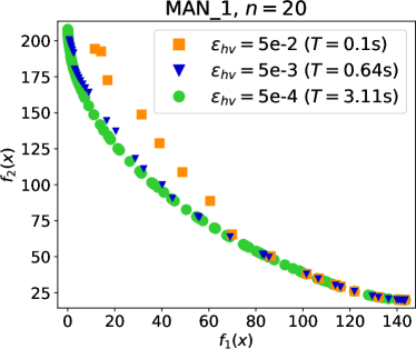
(a)

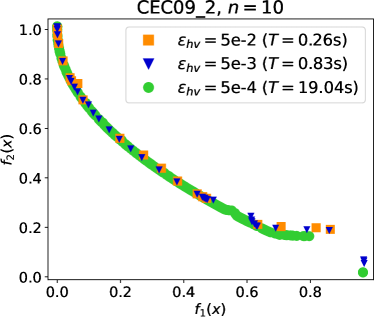
(b)

Figure 3: Pareto front reconstructions by FD-SD on MAN_1 ($n=20$) and CEC09_2 ($n=10$) problems with different values for the Hyper-volume improvement threshold $\varepsilon_{hv}$ (Remark 5.29). For each execution, the runtime $T$ is reported.

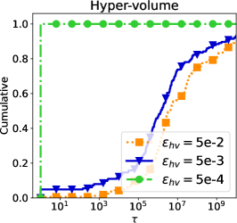
(a)

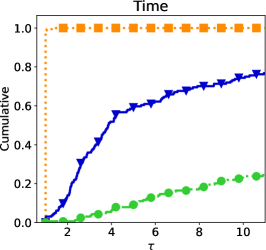
(b)

Figure 4: Performance profiles w.r.t. Hyper-volume and Time for FD-SD on the bi-objective optimization problems listed in Section 6. The axes were set for a better visualization of the results.

6.2 Overall Comparison

After assessing the properties typical of FD methods, we now compare all the FD variants on the set of bi-objective optimization problems listed in Section 6. Given the results in Section 6.1, here we considered $\varepsilon_{hv}=5\times 10^{-4}$ for all the algorithms. In Fig. 5, we show the performance profiles w.r.t. Purity, Time, Hyper-volume and Spread metrics. As for the first metric, we observe that the employment of Newton-type and Barzilai-Borwein directions in the refinement phase actually helps to improve the quality of the Pareto front reconstruction w.r.t. the classical use of steepest descent direction. However, except for FD-BB, the use of additional information on the Newton-type directions led to an higher consumption of resources, as can be observed in the performance profiles w.r.t. Time. Regarding the Hyper-volume and $\Gamma$–spread metrics, we have that FD-N was the best, with FD-BB having a similar performance, especially in robustness. As for $\Delta$–spread, all the methodologies worked equally well.

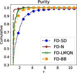
(a)

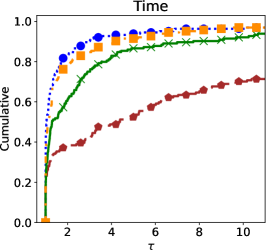
(b)

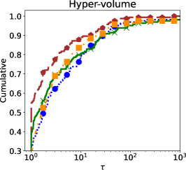
(c)

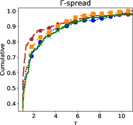
(d)

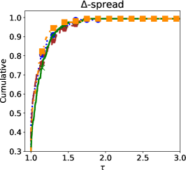
(e)

Figure 5: Performance profiles w.r.t. Purity, Time, Hyper-volume and Spread metrics for FD-SD, FD-N, FD-LMQN, FD-BB on the bi-objective optimization problems listed in Section 6. The axes were set for a better visualization of the results.

For the last comparison, we then decided to use FD-BB, being the best compromise w.r.t. all the metrics. In the comparisons with NSGA-II and MOTR, we run all the algorithms with a time limit of 2 minutes on each problem, being the best stopping criterion to compare such structurally different approaches (of course, any additional stopping condition indicating that an algorithm cannot improve the set of solutions anymore was considered). FD-BB was the clear winner on both Purity and Hyper-volume. Regarding the $\Gamma$–spread, the proposed approach obtained a similar performance as MOTR on effectiveness and appeared to be the most robust algorithm; on $\Delta$–spread, all the algorithms again performed equally well.

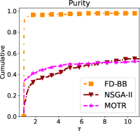
(a)

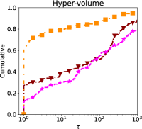
(b)

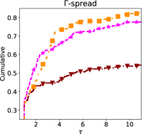
(c)

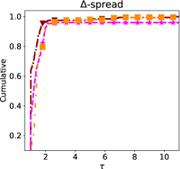
(d)

Figure 6: Performance profiles w.r.t. Purity, Hyper-volume and Spread metrics for FD-BB, NSGA-II and MOTR on all the problems listed in Section 6. The axes were set for a better visualization of the results.

7 Conclusions

In this paper, we introduced the class of Front Descent algorithms for Pareto front reconstruction in smooth multiobjective optimization. For this general class of algorithms, we provided an insightful characterization of its mechanisms, a thorough theoretical analysis of convergence, with some innovative results concerning the sequence of iterate sets, and the experimental evidence of its superiority w.r.t. methods from the state-of-the-art.

The theoretical analysis somehow sheds some light on the strong performance that the algorithm exhibits in terms of the purity metric. Interesting future research might focus on some formal investigation regarding the observed ability of the algorithm to effectively spread the Pareto front - or at least some of its parts in the nonconvex setting. Other research could of course be focused also on adaptations of the framework to the constrained setting.

References

• [1] J. Chen, L. Tang, and X. Yang, Barzilai-Borwein proximal gradient methods for multiobjective composite optimization problems with improved linear convergence, arXiv preprint arXiv:2306.09797, (2023).
• [2] G. Cocchi, M. Lapucci, and P. Mansueto, Pareto front approximation through a multi-objective augmented Lagrangian method, EURO Journal on Computational Optimization, 9 (2021), p. 100008.
• [3] G. Cocchi, G. Liuzzi, S. Lucidi, and M. Sciandrone, On the convergence of steepest descent methods for multiobjective optimization, Computational Optimization and Applications, 77 (2020), pp. 1–27.
• [4] A. L. Custódio, J. A. Madeira, A. I. F. Vaz, and L. N. Vicente, Direct multisearch for multiobjective optimization, SIAM Journal on Optimization, 21 (2011), pp. 1109–1140.
• [5] K. Deb, A. Pratap, S. Agarwal, and T. Meyarivan, A fast and elitist multiobjective genetic algorithm: NSGA-II, IEEE Transactions on Evolutionary Computation, 6 (2002), pp. 182–197.
• [6] E. D. Dolan and J. J. Moré, Benchmarking optimization software with performance profiles, Mathematical Programming, 91 (2002), pp. 201–213.
• [7] G. Eichfelder, Twenty years of continuous multiobjective optimization in the twenty-first century, EURO Journal on Computational Optimization, 9 (2021), p. 100014.
• [8] J. Fliege, L. G. Drummond, and B. F. Svaiter, Newton’s method for multiobjective optimization, SIAM Journal on Optimization, 20 (2009), pp. 602–626.
• [9] J. Fliege and B. F. Svaiter, Steepest descent methods for multicriteria optimization, Mathematical Methods of Operations Research, 51 (2000), pp. 479–494.
• [10] J. Fliege, A. I. F. Vaz, and L. N. Vicente, Complexity of gradient descent for multiobjective optimization, Optimization Methods and Software, 34 (2019), pp. 949–959.
• [11] M. L. Gonçalves, F. S. Lima, and L. Prudente, Globally convergent Newton-type methods for multiobjective optimization, Computational Optimization and Applications, 83 (2022), pp. 403–434.
• [12] J. Handl, D. B. Kell, and J. Knowles, Multiobjective optimization in bioinformatics and computational biology, IEEE/ACM Transactions on Computational Biology and Bioinformatics, 4 (2007), pp. 279–292.
• [13] S. Huband, P. Hingston, L. Barone, and L. While, A review of multiobjective test problems and a scalable test problem toolkit, IEEE Transactions on Evolutionary Computation, 10 (2006), pp. 477–506.
• [14] Y. Jin, M. Olhofer, and B. Sendhoff, Dynamic weighted aggregation for evolutionary multi-objective optimization: Why does it work and how?, in Proceedings of the genetic and evolutionary computation conference, 2001, pp. 1042–1049.
• [15] Y. Jin and B. Sendhoff, Pareto-based multiobjective machine learning: An overview and case studies, IEEE Transactions on Systems, Man, and Cybernetics, Part C (Applications and Reviews), 38 (2008), pp. 397–415.
• [16] R. Lacour, K. Klamroth, and C. M. Fonseca, A box decomposition algorithm to compute the hypervolume indicator, Computers & Operations Research, 79 (2017), pp. 347–360.
• [17] M. Lapucci, Convergence and complexity guarantees for a wide class of descent algorithms in nonconvex multi-objective optimization, Operations Research Letters, 54 (2024), p. 107115.
• [18] M. Lapucci and P. Mansueto, Improved front steepest descent for multi-objective optimization, Operations Research Letters, 51 (2023), pp. 242–247.
• [19] M. Lapucci and P. Mansueto, A limited memory Quasi-Newton approach for multi-objective optimization, Computational Optimization and Applications, 85 (2023), pp. 33–73.
• [20] M. Lapucci, P. Mansueto, and F. Schoen, A memetic procedure for global multi-objective optimization, Mathematical Programming Computation, 15 (2023), pp. 227–267.
• [21] H. Liu, Y. Li, Z. Duan, and C. Chen, A review on multi-objective optimization framework in wind energy forecasting techniques and applications, Energy Conversion and Management, 224 (2020), p. 113324.
• [22] G. Liuzzi, S. Lucidi, and F. Rinaldi, A derivative-free approach to constrained multiobjective nonsmooth optimization, SIAM Journal on Optimization, 26 (2016), pp. 2744–2774.
• [23] L. Lucambio Pérez and L. Prudente, Nonlinear conjugate gradient methods for vector optimization, SIAM Journal on Optimization, 28 (2018), pp. 2690–2720.
• [24] E. Miglierina, E. Molho, and M. Recchioni, Box-constrained multi-objective optimization: A gradient-like method without “a priori” scalarization, European Journal of Operational Research, 188 (2008), pp. 662–682.
• [25] A. Mohammadi and A. Custódio, A trust-region approach for computing Pareto fronts in multiobjective optimization, Computational Optimization and Applications, 87 (2024), pp. 149–179.
• [26] Ž. Povalej, Quasi-Newton’s method for multiobjective optimization, Journal of Computational and Applied Mathematics, 255 (2014), pp. 765–777.
• [27] L. Prudente and D. R. Souza, A quasi-Newton method with Wolfe line searches for multiobjective optimization, Journal of Optimization Theory and Applications, 194 (2022), pp. 1107–1140.
• [28] F. Rosso, V. Ciancio, J. Dell’Olmo, and F. Salata, Multi-objective optimization of building retrofit in the mediterranean climate by means of genetic algorithm application, Energy and Buildings, 216 (2020), p. 109945.
• [29] O. Schütze, A. Lara, and C. C. Coello, The directed search method for unconstrained multi-objective optimization problems, Proceedings of the EVOLVE–A Bridge Between Probability, Set Oriented Numerics, and Evolutionary Computation, (2011), pp. 1–4.
• [30] Q. Zhang, A. Zhou, S. Zhao, P. N. Suganthan, W. Liu, S. Tiwari, et al., Multiobjective optimization test instances for the CEC 2009 special session and competition, University of Essex, Colchester, UK and Nanyang technological University, Singapore, special session on performance assessment of multi-objective optimization algorithms, technical report, 264 (2008), pp. 1–30.
• [31] E. Zitzler and L. Thiele, Multiobjective optimization using evolutionary algorithms — a comparative case study, in Parallel Problem Solving from Nature — PPSN V, A. E. Eiben, T. Bäck, M. Schoenauer, and H.-P. Schwefel, eds., Berlin, Heidelberg, 1998, Springer Berlin Heidelberg, pp. 292–301.