Tackling Prevalent Conditions in Unsupervised Combinatorial Optimization: Cardinality, Minimum, Covering, and More
Abstract
Combinatorial optimization (CO) is naturally discrete, making machine learning based on differentiable optimization inapplicable. Karalias & Loukas (2020) adapted the probabilistic method to incorporate CO into differentiable optimization. Their work ignited the research on unsupervised learning for CO, composed of two main components: probabilistic objectives and derandomization. However, each component confronts unique challenges. First, deriving objectives under various conditions (e.g., cardinality constraints and minimum) is nontrivial. Second, the derandomization process is underexplored, and the existing derandomization methods are either random sampling or naive rounding. In this work, we aim to tackle prevalent (i.e., commonly involved) conditions in unsupervised CO. First, we concretize the targets for objective construction and derandomization with theoretical justification. Then, for various conditions commonly involved in different CO problems, we derive nontrivial objectives and derandomization to meet the targets. Finally, we apply the derivations to various CO problems. Via extensive experiments on synthetic and real-world graphs, we validate the correctness of our derivations and show our empirical superiority w.r.t. both optimization quality and speed.
1 Introduction
Combinatorial optimization (CO) problems are discrete by their nature. Machine learning methods are based on differentiable optimization (e.g., gradient descent), and applying them to CO is non-trivial. In their pioneering work, Karalias & Loukas (2020) adapted the probabilistic method (Erdős & Spencer, 1974; Alon & Spencer, 2016) to incorporate discrete CO problems into differentiable optimization. Specifically, they proposed to evaluate CO objectives on a distribution of discrete choices (i.e., in a probabilistic manner), allowing for the differentiable optimization-based ML techniques to be applied to CO problems. This ignited the line of research on unsupervised (i.e., not supervised by solutions) learning for combinatorial optimization (UL4CO).
There are two components in UL4CO: (1) construction of probabilistic objectives and (2) derandomization to obtain the final discrete solutions. However, the prior works on UL4CO share multiple limitations. First, although some desirable properties of probabilistic objectives (e.g., desirable objectives should be differentiable and align well with the original discrete objectives) have been proposed, how to derive objectives satisfying such properties is still unclear. At the same time, the derandomization process is underexplored, without many practical techniques or theoretical discussions. Specifically, the existing derandomization methods are either random sampling or naive rounding. Random sampling, by its nature, may cost us a large number of samplings (and good luck) to have good results. For naive rounding, the performance may highly depend on the order of rounding and end up with mediocre solutions. They only guarantee, at best, derandomized solutions are no worse than the given continuous solutions w.r.t. the corresponding probabilistic objectives. However, how to obtain stronger guarantees in an efficient way has been an open problem.
Motivated by the limitations, in this work, we focus on objectives and constraints that have not been systematically handled within the UL4CO framework and are commonly involved in various CO problems. We study and propose UCom2 (Usupervised Combinatorial Optimization Under Commonly-involved Conditions). Specifically, our contributions are four-fold.
-
•
We concretize the targets for objective construction and derandomization with theoretical justification (Sec. 3). We theoretically show that probabilistic objectives that can be rephrased as an expectation are desirable, and propose a fast and effective derandomization scheme with a quality guarantee stronger than the existing ones.
-
•
We derive non-trivial objectives and derandomization for various prevalent conditions to meet the targets (Sec. 4). We focus on conditions that are mathematically hard to handle but commonly involved in CO problems, e.g., cardinality constraints, minimum, and covering.
-
•
We apply our derivations to different CO problems involving such prevalent conditions (Sec. 5). For each problem, we analyze what conditions are involved and derive objectives and derandomization by combining our derivations for the involved conditions.
-
•
We show the empirical superiority of UCom2 via experiments (Sec. 6). Equipped with our derivations, our method UCom2 achieves better optimization quality and speed across different CO problems on both synthetic and real-world graphs, outperforming various baselines.
Reproducibility. The code and datasets are available in the online appendix (Bu et al., 2024).111https://github.com/ai4co/unsupervised-CO-ucom2
2 Preliminaries and Background
2.1 Preliminaries
Graphs. A graph is defined by a node set , an edge set , and edge weights . We let denote the number of nodes (WLOG, ), and let denote the number of edges.
Combinatorial optimization (CO). We consider CO problems on graphs with discrete decisions on nodes. Each CO problem can be represented by a tuple with (1) an optimization objective , (2) constraints defined by a feasible set , and (3) a set of possible decisions (on each ). Given decisions with , we have a full decision .
For each graph , we can use the optimization objective function to evaluate each full decision on by , and we aim to solve . By default, we consider CO problems with binary decisions (i.e., ).222We will discuss non-binary cases in Sec. 4.5. Given , we call each node with a chosen node, and call the chosen subset (i.e., the set of chosen nodes).
2.2 Background: UL4CO
We shall introduce the background of unsupervised learning for combinatorial optimization (UL4CO), including the overall pipeline and some existing ideas/techniques.
2.2.1 The UL4CO Pipeline: Erdős Goes Neural
The UL4CO pipeline, Erdős Goes Neural (Karalias & Loukas, 2020), is based on the probabilistic method (Erdős & Spencer, 1974) with three components: objective construction, differentiable optimization, and derandomization.
Probabilistic objective construction. The high-level idea is to evaluate discrete objectives on a distribution of decisions, which accepts continuous parameterization. Specifically, given a CO problem , we first construct a penalized objective with constraint coefficient . Then, a probabilistic objective accepting probabilistic (and thus continuous) inputs is constructed such that
We see each as a vector of probabilities, with ’s being independent Bernoulli variables. Hence, we have
Remark 1.
Differentiable optimization. For differentiable optimization, we need to ensure that is differentiable (w.r.t. ). At this moment, let us assume we have constructed such a . Then, given a graph , we can use differentiable optimization (e.g., gradient descent) to obtain optimized probabilities with (ideally) small .
Derandomization. Finally, derandomization is used to obtain deterministic full decisions. For each test instance , the derandomization process transforms each obtained by probabilistic optimization into a discrete (i.e., deterministic) full decision . Karalias & Loukas (2020) showed a quality guarantee of derandomization by random sampling. See App. B for more details.
2.2.2 Local Derandomization
The theoretical quality guarantee by Karalias & Loukas (2020) is obtained by random sampling, and we may need a large number of samplings (and good luck) to have a good bound. Wang et al. (2022) further proved a deterministic (i.e., not relying on random sampling) quality guarantee by iterative rounding (i.e., a series of local derandomization along with a node enumeration). The principle of iterative rounding involves two concepts: (1) local derandomization of probabilities and (2) entry-wise concavity of probabilistic objective .
Local derandomization. Given , , and , is the result after being locally derandomized as , i.e.,
Entry-wise concavity. A probabilistic objective is entry-wise concave if and ,
.
Applying a series of local derandomization with an entry-wise concave objective does not increase the objective. Notably, Karalias & Loukas (2020) essentially proposed iterative rounding, and Wang et al. (2022) first formalized a theoretical guarantee of iterative rounding with the condition of entry-wise concavity. See App. B for more details.
3 Concretizing Targets: What Do We Need?
First, we concretize the targets for objective construction and derandomization to guide our further derivations.
3.1 Good objectives: Expectations are all you need
Good properties. We summarize some known good properties of a probabilistic objective (Karalias & Loukas, 2020; Wang et al., 2022): (P1) accepts continuous inputs (rather than discrete ); (P2) is an upper bound of the expectation of a penalized objective for some ; (P3) is differentiable w.r.t. ; (P4) is entry-wise concave w.r.t. ; (P5) has the same minimum as , i.e., and . The property (P5) has been discussed (Karalias & Loukas, 2020; Karalias et al., 2022; Kollovieh et al., 2024) but has not been explicitly formalized for UL4CO. With (P5), when we minimize , we also minimize the original objective , which avoids meaningless , e.g., a constant function with a very high value (which satisfies (P1)-(P4) but not (P5)).
Below, we show that a specific form of objectives satisfies all the good properties. First, expectations are all you need, i.e., any probabilistic objective that is the expectation of any discrete function satisfies properties (P1), (P3), and (P4).
Theorem 1 (Expectations are all you need).
For any , with is differentiable and entry-wise concave w.r.t. .
Proof.
See App. A for all the proofs. ∎
Remark 2.
Differentiability and entry-wise concavity are closed under addition. Hence, a linear combination of expectations is also differentiable and entry-wise concave. Also, probabilities are special expectations of indicator functions. The differentiability of expectation may not hold when ’s are not independent Bernoulli variables, e.g., when the expectation is taken with Lovasz extension (Bach et al., 2013).
To further satisfy (P2) and (P5), we only need to find a tight upper bound (TUB) of a penalized objective.
Definition 1 (Tight upper bounds).
Given , we say is a tight upper bound (TUB) of , iff (i.e., if and only if) with and , where .
Remark 3.
It is easy to see that is always a TUB of . When is an indicator function for the violation of constraints , the condition in Def. 1 is equivalent to and .
To conclude, we propose the following concretized target to construct the expectation of a tight upper bound.
Target 1 (Construct the expectation of a TUB).
Given with constraints , let , we aim to find such that is a TUB of and is a TUB of , and to construct a probabilistic objective with .
3.2 Fast and effective derandomization: Do it in a greedy and incremental manner
Greedy. To this end, we generalize greedy algorithms to greedy derandomization and propose an incremental scheme to improve the speed. For greedy derandomization, starting from , we repeat the following steps:
(1) we greedily find the best local derandomization, i.e.,
;
(2) we conduct the best derandomization, i.e.,
.
Theorem 2 (Goodness of greedy derandomization).
For any entry-wise concave and any , the above process of greedy derandomization can always reach a point where the final is (G1) discrete (i.e., ), (G2) no worse than (i.e., ), and (G3) a local minimum (i.e., ).
Remark 4.
Greedy derandomization improves upon the existing derandomization methods. Specifically, random sampling (Karalias & Loukas, 2020) guarantees (G1), and iterative rounding (Wang et al., 2022) guarantees (G1) and (G2). However, challenges arise regarding the time complexity since a naive way requires evaluations of at each step.
Incremental. To this end, we propose to conduct the derandomization in an incremental manner to increase the speed, which gives the following target. Our intuition is that, usually, the incremental differences are simpler than the whole function, and the computation of incremental differences is easily parallelizable.
Target 2 (Conduct incremental greedy derandomization).
We conduct greedy derandomization and improve the speed by deriving the incremental differences (IDs) for all the pairs, instead of evaluating the “whole” function, i.e., ’s.
4 Deriving Formulae to Meet the Targets
The targets in Sec. 3 provide us guidelines, while deriving objectives and derandomization to meet those targets is nontrivial. In this work, we focus on UCom2 (Usupervised Combinatorial Optimization Under Commonly-involved Conditions) and baptize our method with the same name. For various conditions that are commonly involved in different CO problems (see Sec. 5 and App. E), we shall derive (1) TUB-based probabilistic objectives to meet Target 1 and (2) incremental differences (IDs) of to meet Target 2. Some conditions were encountered in the existing works but were not properly handled within the probabilistic UL4CO pipeline. See more discussions in App. B.3.
We tackle each condition using the template below. Note that deriving TUB and IDs for each condition requires distinct, non-trivial ideas.
The conditions to be tackled below have both theoretical and empirical values. Specifically, they are mathematically hard to handle for probabilistic UL4CO, and are commonly involved in many CO problems.
4.1 Cardinality constraints
Definition. We consider constraints with . Some typical cases are or for some (Buchbinder et al., 2014).
Given , (see Sec. 2) follows a Poisson binomial distribution with parameters (Wang, 1993). The probability mass function (PMF) is for each ,
.
(S1-1). We find , i.e., the minimum distance to the feasible cardinality set .
Lemma 1.
is a TUB of .
Remark 5.
We can directly compute , but the formula we use practically performs better, which distinguishes different levels of violations. See similar ideas by, e.g., (Pogancic et al., 2019).
(S1-2). We derive . The main technical difficulty is computing the PMF of a Poisson binomial distribution, for which we adopt a discrete-Fourier-transform-based method. The main formula of (See Eq. (6) by Hong (2013)) is
,
where and . See App. C.1 for more details.
(S2). We derive the IDs of , using the recursive formula of the Poisson binomial distribution.
Lemma 2 (IDs of ).
For any , , and , let and , we have
| (1) | ||||
| (2) |
Based on that, we have
Remark 6.
4.2 Minimum (or maximum) w.r.t. a subset
Definition. We consider constraints where we have a pairwise score function (e.g., distance) and we aim to compute for some (e.g., the shortest distance to a set of points).
We fix in the analysis below, and let be a permutation of such that , where .
(S1-1). We find , which is the original objective .
Lemma 3.
is a TUB of .
(S1-2). We derive , by decomposing the objective into sub-terms.
Lemma 4.
For any , .
(S2). We derive the IDs of , by analyzing which sub-terms are changed after one step of local derandomization.
Lemma 5 (IDs of ).
For any and , let , the coefficient of in . Then
Remark 7.
When , we replace by . Since we make sure each (see Rem. 6), this does not happen in practice.
4.3 Covering
Definition. We consider conditions where some needs to be covered (i.e., at least one neighbor of is chosen). Formally, the constraints are with .
(S1-1). We find , which is the indicative function of the original constraint.
Lemma 6.
is a TUB of .
(S1-2). We drive , by decomposing the objective into sub-terms.
Lemma 7.
For any and , .
(S2). We derive the IDs of , by analyzing which sub-terms are changed after one step of local derandomization.
Lemma 8 (IDs of ).
For any and , if , then ; if , then
4.4 Cliques (or independent sets)
Definition. We consider conditions where the chosen nodes should form a clique.333Equivalently, an independent set in the complement graph. Formally, the constraints are with .
(S1-1). We find , the number of chosen node pairs violating the constraints.
Lemma 9.
is a TUB of .
(S1-2). We derive , by decomposing the objective into sub-terms.
Lemma 10.
For any , .
(S2). We derive the IDs of , by analyzing which sub-terms are changed after one step of local derandomization.
Lemma 11 (IDs of ).
For any and ,
Notes. (Karalias & Loukas, 2020) and (Min et al., 2022) essentially considered the “cliques” conditions and derived similar formula of . Our derivation of the IDs is novel, and we will also extend this to non-binary cases, which were not discussed in existing works. Moreover, our high-level targets and templates provide insights into obtaining and interpreting the derivation in a principled way.
4.5 Non-binary decisions
Definition. We consider non-binary decisions, i.e., (potentially) more than two decisions (), e.g., problems with partition or coloring. Our theoretical analysis can be extended to non-binary cases. See App. D.1 for more details.
4.6 Uncertainty
We also consider uncertainty in edge existence, i.e., edge probabilities . Due to the generality of non-binary conditions and uncertainty, the details of objective construction and derandomization will be deferred to where each specific problem is analyzed in Sec. 5.
4.7 Notes and insights
Throughout the section, two commonly used ideas for constructing TUBs are: (1) using a function itself (Lemmas 3 & 6), and (2) relaxing the binary “a constraint is violated” to “the number of violations” (Lemmas 1 & 9).
Moreover, techniques commonly used in our derivations include (1) decomposing objectives into sub-terms, and (2) analyzing which sub-terms are changed after one step of local derandomization. Such “local decomposibility” allows us to use linearity of expectation. See, e.g., similar ideas by Ahn et al. (2020) and Jo et al. (2023). See App. G.3 for more discussions.
We acknowledge that we have not covered all conditions involved in CO, but we expect that similar ideas would be applicable to some other conditions. See App. E.5 for discussions on some conditions not fully covered in this work, e.g., cycles and trees.
5 Applying the Derivations to CO Problems
In this section, we apply UCom2 to different CO problems (facility location, maximum coverage, and robust coloring) with both theoretical values, NP-hardness (Mihelic & Robic, 2004; Yanez & Ramirez, 2003), and real-world implications. See App. E for the applications to four more problems (robust -clique, robust dominating set, clique cover, and minimum spanning tree). Specifically, for each specific problem, we shall (1) check what conditions are involved and (2) construct the probabilistic objective and derandomization process by combining the analyses in Sec. 4.
5.1 Facility location
The facility location problem is abstracted from real-world scenarios, where the goal is to find some good locations among candidate locations (Drezner & Hamacher, 2004).
Definition. Given (1) a complete weighted graph , where the distance between each pair of nodes is , and , and (2) the number of locations to choose, we aim to find a subset such that (c1) , and (c2) is minimized.
Involved conditions: (1) cardinality constraints and (2) minimum w.r.t. a subset (see Secs. 4.1 & 4.2).
Details. Given and ,
.
For and , the ID is .
5.2 Maximum coverage
The maximum coverage problem (Khuller et al., 1999) is a classical CO problem with real-world applications, including public traffic management (Ali & Dyo, 2017), web management (Saha & Getoor, 2009), and scheduling (Marchiori & Steenbeek, 2000).
Definition. Given (1) items (WLOG, assume the items are ), each with weight , (2) a family of sets with each and (3) the number of sets to choose, we aim to choose from the given sets such that (c1) and (c2) the total weights of the covered items is maximized, where is the set of covered items.
Details. Construct a bipartite graph , where iff . For and ,
.
For and , the ID is .
5.3 Robust coloring
The robust coloring problem (Yanez & Ramirez, 2003) generalizes the coloring problem (Jensen & Toft, 2011). It is motivated by real-world scheduling problems where some conflicts can be uncertain, with notable applications to supply chain management (Lim & Wang, 2005).

Definition. Given (1) an uncertain graph and (2) the number of colors, let represent hard conflicts which we must avoid, and let represent soft conflicts which possibly happen, we aim to find a -coloring on , where each node has a color , such that (c1) no hard conflicts are violated (i.e., ), and (c2) the probability that no violated soft conflicts happen (i.e., ) is maximized.
We fix and in the analysis below.
Involved conditions: (1) independent sets,444The nodes in each color group should be an independent set. (2) uncertainty, and (3) non-binary decisions (see Secs. 4.4 to 4.6).
Details. Regarding (c1), we extend the derivations in Sec. 4.4 to non-binary cases. We use
,
which is a TUB of with , and use . Regarding (c2), maximizing is equivalent to minimizing
.
With and , the final objective is with constraint coefficient .
Lemma 12.
is a TUB of and is a TUB of .
We derive each term in as follows.
Lemma 13.
For any , and with
,
and .
Proof sketch.
We extend the ideas in Lemma 10. ∎
We then derive the IDs of each term in .
Lemma 14 (IDs of the terms in ).
For any , , and ,
, and .
Proof sketch.
We extend the ideas in Lemma 11. Changing only affects with , and we compute the differences for each . ∎
We finally get the overall IDs .
Notes. When practitioners encounter new problems that involve the conditions covered in this work, they can simply combine our derivations for the involved conditions, just as we did in this section. Indeed, we believe many other CO problems involve the conditions considered in this work.
6 Experiments
Through extensive experiments on various problems, we shall show the effectiveness of UCom2.
6.1 Facility location and maximum coverage
We conduct experiments on the facility location problem and the maximum coverage problem (Secs. 5.1 & 5.2). For the experimental settings, we mainly follow an existing work (Wang et al., 2023), with additional datasets and baselines. For fair comparisons, we consider inductive settings (training and test sets are different) and use the same GNN architectures as Wang et al. (2023). See App. G.1 for discussions on transductive settings. See App. F.1 for the detailed experimental settings.
| Method | rand500 | rand800 | starbucks | mcd | subway | average | average rank \bigstrut | ||||||||
| obj | time | obj | time | obj | time | obj | time | obj | time | obj | time | obj | time | sum \bigstrut | |
| random | 1.43 | 263.29 | 1.51 | 125.65 | 1.86 | 461.54 | 1.64 | 122.45 | 1.52 | 119.40 | 1.61 | 240.34 | 11.6 | 13.6 | 25.2 \bigstrut[t] |
| greedy | 1.19 | 2.30 | 1.16 | 3.08 | 1.21 | 12.52 | 1.19 | 5.87 | 1.11 | 12.94 | 1.17 | 7.34 | 8.6 | 4.0 | 12.6 |
| Gurobi | 1.07 | 133.68 | 1.26 | 65.47 | 1.07 | 197.08 | 1.51 | 63.88 | 2.63 | 69.08 | 1.51 | 105.84 | 9.0 | 11.8 | 20.8 |
| SCIP | 1.73 | 103.55 | 2.35 | 100.34 | 19.76 | 154.83 | 55.10 | 247.91 | 55.01 | 366.47 | 26.79 | 194.62 | 15.8 | 12.8 | 28.6 |
| CardNN-S | 1.14 | 15.29 | 1.06 | 8.45 | 1.62 | 36.98 | 1.16 | 11.99 | 1.08 | 10.14 | 1.21 | 16.57 | 7.4 | 5.4 | 12.8 |
| CardNN-GS | 1.00 | 78.38 | 1.01 | 74.22 | 1.07 | 76.69 | 1.15 | 21.60 | 1.03 | 14.99 | 1.05 | 53.18 | 4.0 | 9.0 | 13.0 |
| CardNN-HGS | 1.00 | 110.14 | 1.01 | 95.11 | 1.07 | 174.87 | 1.15 | 49.20 | 1.02 | 28.48 | 1.05 | 91.56 | 3.4 | 11.2 | 14.6 |
| CardNN-noTTO-S | 1.43 | 2.23 | 1.55 | 1.05 | 3.34 | 3.90 | 3.90 | 1.00 | 3.54 | 1.00 | 2.75 | 1.84 | 14.0 | 1.6 | 15.6 |
| CardNN-noTTO-GS | 1.14 | 31.39 | 1.15 | 27.18 | 1.52 | 15.73 | 1.26 | 8.03 | 1.23 | 2.21 | 1.26 | 16.91 | 8.8 | 4.8 | 13.6 |
| CardNN-noTTO-HGS | 1.14 | 40.97 | 1.15 | 32.30 | 1.45 | 29.98 | 1.27 | 14.44 | 1.21 | 3.67 | 1.24 | 24.27 | 8.4 | 6.6 | 15.0 |
| EGN-naïve | 1.10 | 86.45 | 1.14 | 44.66 | 1.14 | 232.44 | 1.66 | 24.53 | 1.47 | 60.13 | 1.30 | 89.64 | 8.6 | 10.6 | 19.2 |
| RL-transductive | 2.32 | 329.11 | 2.24 | 157.07 | 10.24 | 3461.54 | 2.77 | 918.37 | 2.51 | 895.52 | 4.02 | 1152.32 | 14.6 | 15.6 | 30.2 |
| RL-inductive | 1.70 | 329.17 | 1.85 | 157.35 | 2.72 | 577.00 | 2.55 | 153.08 | 2.36 | 149.28 | 2.24 | 273.18 | 13.2 | 15.0 | 28.2 \bigstrut[b] |
| UCom2-short | 1.05 | 1.00 | 1.03 | 1.00 | 1.03 | 1.00 | 1.05 | 1.31 | 1.04 | 1.77 | 1.04 | 1.89 | 4.2 | 1.4 | 5.6 \bigstrut[t] |
| UCom2-middle | 1.00 | 32.56 | 1.00 | 15.65 | 1.03 | 4.35 | 1.01 | 4.47 | 1.01 | 13.05 | 1.01 | 14.02 | 2.0 | 4.8 | 6.8 |
| UCom2-long | 1.00 | 81.03 | 1.00 | 31.12 | 1.00 | 20.27 | 1.00 | 19.41 | 1.00 | 22.88 | 1.00 | 34.94 | 1.0 | 7.8 | 8.8 \bigstrut[b] |
| Method | rand500 | rand1000 | twitch | railway | average | average rank \bigstrut | |||||||
| obj | time | obj | time | obj | time | obj | time | obj | time | obj | time | sum \bigstrut | |
| random | 0.82 | 2666.67 | 0.79 | 727.27 | 0.52 | 369.23 | 0.96 | 315.79 | 0.77 | 1019.74 | 12.8 | 14.0 | 26.8 \bigstrut[t] |
| greedy | 0.98 | 1.00 | 0.99 | 1.00 | 1.00 | 1.06 | 1.00 | 1.00 | 0.99 | 1.02 | 7.3 | 1.3 | 8.5 |
| Gurobi | 1.00 | 1333.89 | 1.00 | 363.94 | 1.00 | 1.00 | 1.00 | 158.87 | 1.00 | 464.42 | 3.3 | 8.8 | 12.0 |
| SCIP | 0.97 | 1334.11 | 0.96 | 362.09 | 1.00 | 5.05 | 1.00 | 159.84 | 0.98 | 465.27 | 6.3 | 10.8 | 17.0 |
| CardNN-S | 0.93 | 130.33 | 0.93 | 35.94 | 1.00 | 12.25 | 0.97 | 3.71 | 0.96 | 45.56 | 8.0 | 5.5 | 13.5 |
| CardNN-GS | 0.99 | 448.11 | 1.00 | 169.55 | 1.00 | 25.38 | 1.00 | 23.21 | 1.00 | 166.56 | 4.3 | 9.0 | 13.3 |
| CardNN-HGS | 0.99 | 618.22 | 1.00 | 248.33 | 1.00 | 47.28 | 1.00 | 35.86 | 1.00 | 237.42 | 3.3 | 10.5 | 13.8 |
| CardNN-noTTO-S | 0.70 | 20.33 | 0.69 | 6.18 | 0.01 | 1.43 | 0.94 | 1.54 | 0.58 | 7.37 | 16.0 | 2.8 | 18.8 |
| CardNN-noTTO-GS | 0.82 | 115.56 | 0.79 | 61.18 | 0.02 | 2.97 | 0.96 | 7.53 | 0.65 | 46.81 | 13.5 | 5.0 | 18.5 |
| CardNN-noTTO-HGS | 0.82 | 132.56 | 0.79 | 75.15 | 0.19 | 3.62 | 0.96 | 12.14 | 0.69 | 55.87 | 12.3 | 6.5 | 18.8 |
| EGN-naive | 0.92 | 1334.56 | 0.91 | 364.45 | 0.13 | 185.22 | 0.97 | 159.13 | 0.73 | 510.84 | 11.3 | 12.8 | 24.0 |
| RL-transductive | 0.92 | 3333.33 | 0.82 | 909.09 | 0.95 | 2769.23 | 0.96 | 2368.42 | 0.91 | 2345.02 | 11.5 | 15.5 | 27.0 |
| RL-inductive | 0.77 | 3334.00 | 0.77 | 909.64 | 0.59 | 464.48 | 0.96 | 397.08 | 0.77 | 1276.30 | 13.8 | 15.5 | 29.3 \bigstrut[b] |
| UCom2-short | 0.99 | 10.67 | 0.99 | 5.55 | 1.00 | 2.80 | 1.00 | 2.63 | 1.00 | 5.41 | 5.8 | 2.8 | 8.5 \bigstrut[t] |
| UCom2-middle | 1.00 | 168.44 | 1.00 | 23.76 | 1.00 | 17.58 | 1.00 | 10.75 | 1.00 | 55.13 | 3.8 | 6.5 | 10.3 |
| UCom2-long | 1.00 | 333.56 | 1.00 | 222.85 | 1.00 | 29.77 | 1.00 | 21.11 | 1.00 | 151.82 | 2.3 | 9.0 | 11.3 \bigstrut[b] |
Methods. We compare UCom2 with: (1) random: locations or sets are picked uniformly at random; (2) greedy: deterministic greedy algorithms; (3-4) Gurobi (Gurobi Optimization, LLC, 2023) and SCIP (Bestuzheva et al., 2021; Perron & Furnon, 2023): the problems are formulated as MIPs and the two solvers are used; (5) CardNN (Wang et al., 2023): a SOTA UL4CO method with three variants; (6) CardNN-noTTO: CardNN directly optimizes on each test graph in test time, and these are variants of CardNN without test-time optimization; (7) EGN-naive: EGN (Karalias & Loukas, 2020) with a naive probabilistic objective construction and iterative rounding; (8) RL: a reinforcement-learning method (Kool et al., 2019). See App. G.2 for discussions on reinforcement learning.
| Method | collins, 18 colors | collins, 25 colors | gavin, 8 colors | gavin, 15 colors | krogan, 8 colors | krogan, 15 colors | ppi, 47 colors | ppi, 50 colors | average rank \bigstrut | ||||||||||
| obj | time | obj | time | obj | time | obj | time | obj | time | obj | time | obj | time | obj | time | obj | time | sum \bigstrut | |
| greedy-RD | 115.33 | 300.34 | 23.42 | 300.79 | 66.51 | 300.53 | 7.36 | 301.46 | 117.47 | 300.06 | 0.87 | 301.24 | 4.16 | 301.31 | 1.23 | 301.24 | 2.88 | 3.25 | 6.13 \bigstrut[t] |
| greedy-GA | 114.36 | 188.21 | 22.20 | 243.93 | 66.51 | 398.90 | 7.36 | 540.62 | 117.47 | 941.35 | 0.87 | 1256.66 | 3.66 | 1416.38 | 1.23 | 1484.27 | 2.50 | 4.25 | 6.75 |
| DC | 586.56 | 300.28 | 159.15 | 300.38 | 311.91 | 300.11 | 58.10 | 300.12 | 1065.52 | 300.07 | 1.76 | 300.46 | 43.35 | 300.13 | 6.72 | 300.76 | 5.00 | 2.50 | 7.50 |
| Gurobi | 87.28 | 301.71 | 16.23 | 306.10 | 42.41 | 300.80 | 7.28 | 303.50 | 46.78 | 300.80 | 0.87 | 51.70 | 4.60 | 328.48 | 1.31 | 313.23 | 2.50 | 4.00 | 6.50 |
| UCom2 (CPU) | 82.26 | 79.36 | 15.16 | 54.37 | 42.99 | 152.20 | 6.72 | 260.90 | 53.44 | 211.43 | 0.87 | 8.55 | 2.93 | 116.54 | 1.01 | 120.56 | 1.50 | 1.00 | 2.50 \bigstrut[t] |
| UCom2 (GPU) | 7.09 | 8.03 | 13.28 | 17.25 | 13.73 | 1.91 | 5.24 | 5.48 | \bigstrut[b] | ||||||||||
Datasets. We consider both synthetic and real-world graphs.
-
•
Random graphs: The number after “rand” represents the size of the random graphs. Each group of random graphs contains 100 graphs from the same distribution.
-
•
Real-world graphs: For facility location, each graph contains real-world entities with locations (starbucks, mcd, subway). For maximum coverage, each graph contains real-world sets (twitch, railway). Each group of real-world graphs contains multiple graphs from the same source.
Speed-quality trade-offs. For several methods (including UCom2), we can grant more running time to obtain better optimization quality. For UCom2, we use test-time augmentation (Jin et al., 2023) on the test graphs by adding perturbations into graph topology and features. UCom2-short does not test-time augmentation, while the other two variants use different numbers of augmented data.
Evaluation. For each group of datasets and each method, we report the average optimization objective and running time over five trials. We also report the overall objective, time, and ranks, averaged over all the groups of datasets. The average rank “sum” (ARS) is the summation of the average ranks w.r.t. objective and time. See App. F for the full results with standard deviations and ablation studies.
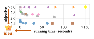
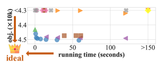
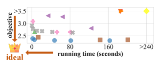
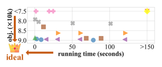
Results. On both problems, UCom2 achieves the best trade-offs overall (Tables 1 & 2). On facility location, the top- methods w.r.t. ARS are the three variants of UCom2. On maximum coverage, the three variants rank 1, 3, and 4 w.r.t. ARS, respectively. In Figure 1, we report the detailed trade-offs of different methods on the random graphs, visually illustrating the best trade-off overall by UCom2.
6.2 Robust coloring
We conduct experiments on the robust coloring problem (see Sec. 5.3) under transductive settings directly optimizing probabilistic decisions . See App. F.1 for more details.
Methods. We compare UCom2 with four baseline methods. (1-2) Greedy-RD and greedy-GA: both methods decide the colors following an enumeration of nodes, where greedy-RD follows a random (RD) permutation of the nodes while greedy-GA uses a genetic algorithm (GA) to learn the permutation;555Greedy-GA is the method proposed by (Yanez & Ramirez, 2003) in the original paper of robust coloring. (3) Deterministic coloring (DC): a deterministic greedy coloring algorithm (Kosowski & Manuszewski, 2004) is used to avoid all the hard conflicts, and it tries to avoid as many soft conflicts as possible; (4) Gurobi: the problem is formulated as an MIP and the solver is used.
Datasets. We use four real-world uncertain graphs: (1) collins, (2) gavin, (3) krogan, and (4) PPI.
Speed-quality trade-offs. We record the running time of UCom2 using only CPUs and using GPUs. For UCom2, we use multiple initial probabilities. We make sure that even with only CPUs, UCom2 uses less time than each baseline.
Evaluation. For each group of datasets and each method, we report the average optimization objective and running time over five trials. The average ranks are computed in the same way as for facility location and maximum coverage.
Results. As shown in Table 3, with the least running time, UCom2 consistently achieves (1) better optimization quality than the two greedy baselines and DC and (2) better optimization quality than Gurobi in most cases. This superiority holds even when we only use CPUs for UCom2. When using GPUs, UCom2 is even faster.
6.3 Ablation studies
We analyze different components in UCom2 and show that (1) good probabilistic objectives are helpful, (2) greedy derandomization is more effective than iterative rounding, and (3) incremental derandomization improves the speed. See App. F.3 for more details.
7 General Related Work: Learning for CO
We shall discuss more general related works, including other learning-based methods for CO problems.
Reinforcement learning for CO. Typical techniques include reinforcement learning (RL). The pioneers who applied RL to CO include (Bello et al., 2016) and (Khalil et al., 2017). Most reinforcement-learning-for-combinatorial-optimization methods focus on routing problems such as the traveling salesman problem (TSP) and the vehicle routing problem (VRP) (Berto et al., 2023; Kool et al., 2019; Kim et al., 2021; Delarue et al., 2020; Qiu et al., 2022; Nazari et al., 2018; Ye et al., 2023a; Chalumeau et al., 2023; Luo et al., 2023; Grinsztajn et al., 2023; Ye et al., 2024; Xiao et al., 2024), as well as maximum independent sets (MIP) (Ahn et al., 2020; Qiu et al., 2022; Sun & Yiming, 2023; Li et al., 2023b). See also some recent surveys on RL4CO (Mazyavkina et al., 2021; Bengio et al., 2021; Cappart et al., 2023; Munikoti et al., 2023) for more details. The existing RL-based methods still suffer from efficiency issues. See the discussions by (Wang et al., 2022) and (Wang et al., 2023). See also App. G.2 for more discussions.
Other machine-learning techniques for CO. Some other machine-learning techniques have been proposed for CO. There is recent progress based on search (Choo et al., 2022; Son et al., 2023; Li et al., 2023b), sampling (Sun et al., 2023), graph-based diffusion (Sun & Yiming, 2023), generative flow networks (Zhang et al., 2023), meta-learning (Qiu et al., 2022; Wang & Li, 2023), and quantum machine learning (Ye et al., 2023b). Physics-inspired machine learning has also been considered by researchers (Schuetz et al., 2022a; Aramon et al., 2019; Schuetz et al., 2022b). There is also a line of research on perturbation-based methods for CO (Pogancic et al., 2019; Berthet et al., 2020; Paulus et al., 2021; Ferber et al., 2023).
8 Conclusion and Discussion
In this work, we study and propose UCom2 (Usupervised Combinatorial Optimization Under Commonly-involved Conditions). Specifically, we concretize the targets for probabilistic objective construction and derandomization (Sec. 3) with theoretical justification (Theorems 1 and 2), derive non-trivial objectives and derandomization for various conditions (e.g., cardinality constraints and minimum) to meet the targets (Sec. 4; Lemmas 1 to 11), apply the derivations to different problems involving such conditions (Sec. 5), and finally show the empirical superiority of our method via extensive experiments (Sec. 6). For reproducibility, we share the code and datasets online (Bu et al., 2024).
As discussed in Sec. 4.7, we have not covered all conditions involved in CO in this work, while we believe that our high-level ideas are applicable to other conditions and problems. The performance of UCom2 and general UL4CO on other conditions (Min et al., 2023; Lachapelle et al., 2020) and hard instances (Xu et al., 2007; Li et al., 2023a) are interesting topics for future exploration.
Acknowledgments
The authors thank all the anonymous reviewers for their helpful comments.
The authors thank Dr. Runzhong Wang @ MIT, Federico Berto @ KAIST, Chuanbo Hua @ KAIST, and Dr. Junyoung Park @ Qualcomm for constructive discussions.
Fanchen Bu gives special thanks to Prof. Jaehoon Kim @ KAIST, Dr. Hong Liu @ IBS, and Yuhao Yao @ Huawei from whom Fanchen Bu studied the probabilistic method.
This work was supported by Institute of Information & Communications Technology Planning & Evaluation (IITP) grant funded by the Korea government (MSIT) (No. 2022-0-00871, Development of AI Autonomy and Knowledge Enhancement for AI Agent Collaboration) (No. 2019-0-00075, Artificial Intelligence Graduate School Program (KAIST)) (No. 2019-0-01906, Artificial Intelligence Graduate School Program (POSTECH)).
Impact Statement
This paper presents work whose goal is to advance the field of Machine Learning, especially Machine Learning for Combinatorial Optimization. There are many potential societal consequences of our work, none of which we feel must be specifically highlighted here.
References
- Ahn et al. (2020) Ahn, S., Seo, Y., and Shin, J. Learning what to defer for maximum independent sets. In ICML, 2020.
- Ali & Dyo (2017) Ali, J. and Dyo, V. Coverage and mobile sensor placement for vehicles on predetermined routes: A greedy heuristic approach. In WINSYS, 2017.
- Alon & Spencer (2016) Alon, N. and Spencer, J. H. The probabilistic method. John Wiley & Sons, 2016.
- Aramon et al. (2019) Aramon, M., Rosenberg, G., Valiante, E., Miyazawa, T., Tamura, H., and Katzgraber, H. G. Physics-inspired optimization for quadratic unconstrained problems using a digital annealer. Frontiers in Physics, 7:48, 2019.
- Bach et al. (2013) Bach, F. et al. Learning with submodular functions: A convex optimization perspective. Foundations and Trends® in machine learning, 6(2-3):145–373, 2013.
- Bello et al. (2016) Bello, I., Pham, H., Le, Q. V., Norouzi, M., and Bengio, S. Neural combinatorial optimization with reinforcement learning. In ICLR, 2016.
- Bengio et al. (2021) Bengio, Y., Lodi, A., and Prouvost, A. Machine learning for combinatorial optimization: a methodological tour d’horizon. European Journal of Operational Research, 290(2):405–421, 2021.
- Berthet et al. (2020) Berthet, Q., Blondel, M., Teboul, O., Cuturi, M., Vert, J.-P., and Bach, F. Learning with differentiable pertubed optimizers. In NeurIPS, 2020.
- Berto et al. (2023) Berto, F., Hua, C., Park, J., Kim, M., Kim, H., Son, J., Kim, H., Kim, J., and Park, J. RL4CO: an extensive reinforcement learning for combinatorial optimization benchmark. arXiv:2306.17100, 2023.
- Bestuzheva et al. (2021) Bestuzheva, K., Besançon, M., Chen, W.-K., Chmiela, A., Donkiewicz, T., van Doornmalen, J., Eifler, L., Gaul, O., Gamrath, G., Gleixner, A., et al. The scip optimization suite 8.0. arXiv 2112.08872, 2021.
- Billionnet (2005) Billionnet, A. Different formulations for solving the heaviest k-subgraph problem. INFOR: Information Systems and Operational Research, 43(3):171–186, 2005.
- Bomze et al. (1999) Bomze, I. M., Budinich, M., Pardalos, P. M., and Pelillo, M. The maximum clique problem. Handbook of Combinatorial Optimization: Supplement Volume A, pp. 1–74, 1999.
- Bu et al. (2024) Bu, F., Jo, H., Lee, S. Y., Ahn, S., and Shin, K. Tackling prevalent conditions in unsupervised combinatorial optimization: Code and datasets. https://github.com/ai4co/unsupervised-CO-ucom2, 2024.
- Buchbinder et al. (2014) Buchbinder, N., Feldman, M., Naor, J., and Schwartz, R. Submodular maximization with cardinality constraints. In SODA, 2014.
- Cappart et al. (2023) Cappart, Q., Chételat, D., Khalil, E. B., Lodi, A., Morris, C., and Velickovic, P. Combinatorial optimization and reasoning with graph neural networks. J. Mach. Learn. Res., 24:130–1, 2023.
- Caprara et al. (2000) Caprara, A., Toth, P., and Fischetti, M. Algorithms for the set covering problem. Annals of Operations Research, 98(1-4):353–371, 2000.
- Ceccarello et al. (2017) Ceccarello, M., Fantozzi, C., Pietracaprina, A., Pucci, G., and Vandin, F. Clustering uncertain graphs. In PVLDB, 2017.
- Ceria et al. (1998) Ceria, S., Nobili, P., and Sassano, A. A lagrangian-based heuristic for large-scale set covering problems. Mathematical Programming, 81:215–228, 1998.
- Chalumeau et al. (2023) Chalumeau, F., Surana, S., Bonnet, C., Grinsztajn, N., Pretorius, A., Alexandre, L., and Barrett, T. Combinatorial optimization with policy adaptation using latent space search. In NeurIPS, 2023.
- Chen et al. (2019) Chen, X., Chen, M., Shi, W., Sun, Y., and Zaniolo, C. Embedding uncertain knowledge graphs. In AAAI, 2019.
- Choo et al. (2022) Choo, J., Kwon, Y.-D., Kim, J., Jae, J., Hottung, A., Tierney, K., and Gwon, Y. Simulation-guided beam search for neural combinatorial optimization. In NeurIPS, 2022.
- Delarue et al. (2020) Delarue, A., Anderson, R., and Tjandraatmadja, C. Reinforcement learning with combinatorial actions: An application to vehicle routing. In NeurIPS, 2020.
- Diaby (2006) Diaby, M. The traveling salesman problem: a linear programming formulation. arXiv preprint cs/0609005, 2006.
- Drakulic et al. (2023) Drakulic, D., Michel, S., Mai, F., Sors, A., and Andreoli, J.-M. Bq-nco: Bisimulation quotienting for generalizable neural combinatorial optimization. In NeurIPS, 2023.
- Drezner & Hamacher (2004) Drezner, Z. and Hamacher, H. W. Facility location: applications and theory. Springer Science & Business Media, 2004.
- Erdős & Spencer (1974) Erdős, P. and Spencer, J. Probabilistic methods in combinatorics. Akadémiai Kindó, 1974.
- Feige et al. (2001) Feige, U., Peleg, D., and Kortsarz, G. The dense k-subgraph problem. Algorithmica, 29:410–421, 2001.
- Ferber et al. (2023) Ferber, A. M., Huang, T., Zha, D., Schubert, M., Steiner, B., Dilkina, B., and Tian, Y. Surco: Learning linear surrogates for combinatorial nonlinear optimization problems. In ICML, 2023.
- Gaile et al. (2022) Gaile, E., Draguns, A., Ozoliņš, E., and Freivalds, K. Unsupervised training for neural tsp solver. In LION, 2022.
- Graham & Hell (1985) Graham, R. L. and Hell, P. On the history of the minimum spanning tree problem. Annals of the History of Computing, 7(1):43–57, 1985.
- Gramm et al. (2009) Gramm, J., Guo, J., Hüffner, F., and Niedermeier, R. Data reduction and exact algorithms for clique cover. Journal of Experimental Algorithmics (JEA), 13:2–2, 2009.
- Grinsztajn et al. (2023) Grinsztajn, N., Daniel, F.-B., Shikha, S., Bonnet, C., and Barrett, T. Winner takes it all: Training performant RL populations for combinatorial optimization. In NeurIPS, 2023.
- Guha & Khuller (1998) Guha, S. and Khuller, S. Approximation algorithms for connected dominating sets. Algorithmica, 20:374–387, 1998.
- Gurobi Optimization, LLC (2023) Gurobi Optimization, LLC. Gurobi Optimizer Reference Manual, 2023. URL https://www.gurobi.com.
- Hong (2013) Hong, Y. On computing the distribution function for the poisson binomial distribution. Computational Statistics & Data Analysis, 59:41–51, 2013.
- Hu et al. (2017) Hu, J., Cheng, R., Huang, Z., Fang, Y., and Luo, S. On embedding uncertain graphs. In CIKM, 2017.
- Jensen & Toft (2011) Jensen, T. R. and Toft, B. Graph coloring problems. John Wiley & Sons, 2011.
- Jin et al. (2023) Jin, W., Zhao, T., Ding, J., Liu, Y., Tang, J., and Shah, N. Empowering graph representation learning with test-time graph transformation. In ICLR, 2023.
- Jo et al. (2023) Jo, H., Bu, F., and Shin, K. Robust graph clustering via meta weighting for noisy graphs. In CIKM, 2023.
- Karalias & Loukas (2020) Karalias, N. and Loukas, A. Erdos goes neural: an unsupervised learning framework for combinatorial optimization on graphs. In NeurIPS, 2020.
- Karalias et al. (2022) Karalias, N., Robinson, J., Loukas, A., and Jegelka, S. Neural set function extensions: Learning with discrete functions in high dimensions. In NeurIPS, 2022.
- Khalil et al. (2017) Khalil, E., Dai, H., Zhang, Y., Dilkina, B., and Song, L. Learning combinatorial optimization algorithms over graphs. In NeurIPS, 2017.
- Khuller et al. (1999) Khuller, S., Moss, A., and Naor, J. S. The budgeted maximum coverage problem. Information processing letters, 70(1):39–45, 1999.
- Kim et al. (2021) Kim, M., Park, J., et al. Learning collaborative policies to solve NP-hard routing problems. In NeurIPS, 2021.
- Kollovieh et al. (2024) Kollovieh, M., Charpentier, B., Zügner, D., and Günnemann, S. Expected probabilistic hierarchies, 2024. URL https://openreview.net/forum?id=Q3Foe1fDjh.
- Kool et al. (2019) Kool, W., Van Hoof, H., and Welling, M. Attention, learn to solve routing problems! In ICLR, 2019.
- Kosowski & Manuszewski (2004) Kosowski, A. and Manuszewski, K. Classical coloring of graphs. Contemporary Mathematics, 352:1–20, 2004.
- Lachapelle et al. (2020) Lachapelle, S., Brouillard, P., Deleu, T., and Lacoste-Julien, S. Gradient-based neural dag learning. In ICLR, 2020.
- Li et al. (2023a) Li, Y., Chen, X., Guo, W., Li, X., Luo, W., Huang, J., Zhen, H.-L., Yuan, M., and Yan, J. HardSATGEN: Understanding the difficulty of hard sat formula generation and a strong structure-hardness-aware baseline. In KDD, 2023a.
- Li et al. (2023b) Li, Y., Guo, J., Wang, R., and Yan, J. T2T: From distribution learning in training to gradient search in testing for combinatorial optimization. In NeurIPS, 2023b.
- Lim & Wang (2005) Lim, A. and Wang, F. Robust graph coloring for uncertain supply chain management. In HICSS, 2005.
- Luo et al. (2023) Luo, F., Lin, X., Liu, F., Zhang, Q., and Wang, Z. Neural combinatorial optimization with heavy decoder: Toward large scale generalization. In NeurIPS, 2023.
- Marchiori & Steenbeek (2000) Marchiori, E. and Steenbeek, A. An evolutionary algorithm for large scale set covering problems with application to airline crew scheduling. In Workshops on Real-World Applications of Evolutionary Computation, 2000.
- Mazyavkina et al. (2021) Mazyavkina, N., Sviridov, S., Ivanov, S., and Burnaev, E. Reinforcement learning for combinatorial optimization: A survey. Computers & Operations Research, 134:105400, 2021.
- Mihelic & Robic (2004) Mihelic, J. and Robic, B. Facility location and covering problems. In Proc. of the 7th International Multiconference Information Society, volume 500, 2004.
- Min et al. (2022) Min, Y., Wenkel, F., Perlmutter, M., and Wolf, G. Can hybrid geometric scattering networks help solve the maximum clique problem? In NeurIPS, 2022.
- Min et al. (2023) Min, Y., Bai, Y., and Gomes, C. P. Unsupervised learning for solving the travelling salesman problem. In NeurIPS, 2023.
- Miryoosefi & Jin (2022) Miryoosefi, S. and Jin, C. A simple reward-free approach to constrained reinforcement learning. In ICML, 2022.
- Munikoti et al. (2023) Munikoti, S., Agarwal, D., Das, L., Halappanavar, M., and Natarajan, B. Challenges and opportunities in deep reinforcement learning with graph neural networks: A comprehensive review of algorithms and applications. IEEE Transactions on Neural Networks and Learning Systems, 2023.
- Nazari et al. (2018) Nazari, M., Oroojlooy, A., Snyder, L., and Takác, M. Reinforcement learning for solving the vehicle routing problem. In NeurIPS, 2018.
- Papp et al. (2021) Papp, P. A., Martinkus, K., Faber, L., and Wattenhofer, R. DropGNN: Random dropouts increase the expressiveness of graph neural networks. In NeurIPS, 2021.
- Paulus et al. (2021) Paulus, A., Rolínek, M., Musil, V., Amos, B., and Martius, G. CombOptNet: Fit the right np-hard problem by learning integer programming constraints. In ICML, 2021.
- Perron & Furnon (2023) Perron, L. and Furnon, V. Or-tools v9.7, 2023. URL https://developers.google.com/optimization/.
- Pettie & Ramachandran (2002) Pettie, S. and Ramachandran, V. An optimal minimum spanning tree algorithm. Journal of the ACM (JACM), 49(1):16–34, 2002.
- Pogancic et al. (2019) Pogancic, M. V., Paulus, A., Musil, V., Martius, G., and Rolinek, M. Differentiation of blackbox combinatorial solvers. In ICLR, 2019.
- Qiu et al. (2022) Qiu, R., Sun, Z., and Yang, Y. DIMES: A differentiable meta solver for combinatorial optimization problems. In NeurIPS, 2022.
- Rozemberczki et al. (2021) Rozemberczki, B., Allen, C., and Sarkar, R. Multi-scale attributed node embedding. Journal of Complex Networks, 9(2):cnab014, 2021.
- Saha & Getoor (2009) Saha, B. and Getoor, L. On maximum coverage in the streaming model & application to multi-topic blog-watch. In SDM, 2009.
- Sanokowski et al. (2023) Sanokowski, S., Berghammer, W., Hochreiter, S., and Lehner, S. L. Variational annealing on graphs for combinatorial optimization. In NeurIPS, 2023.
- Schuetz et al. (2022a) Schuetz, M. J., Brubaker, J. K., and Katzgraber, H. G. Combinatorial optimization with physics-inspired graph neural networks. Nature Machine Intelligence, 4(4):367–377, 2022a.
- Schuetz et al. (2022b) Schuetz, M. J., Brubaker, J. K., Zhu, Z., and Katzgraber, H. G. Graph coloring with physics-inspired graph neural networks. Physical Review Research, 4(4):043131, 2022b.
- Shu et al. (2022) Shu, J., Xi, B., Li, Y., Wu, F., Kamhoua, C., and Ma, J. Understanding dropout for graph neural networks. In TheWebConf (WWW), 2022.
- Sinkhorn & Knopp (1967) Sinkhorn, R. and Knopp, P. Concerning nonnegative matrices and doubly stochastic matrices. Pacific Journal of Mathematics, 21(2):343–348, 1967.
- Son et al. (2023) Son, J., Kim, M., Kim, H., and Park, J. Meta-sage: Scale meta-learning scheduled adaptation with guided exploration for mitigating scale shift on combinatorial optimization. In ICML, 2023.
- Straka (2017) Straka, M. Poisson binomial distribution for python (github repository). https://github.com/tsakim/poibin, 2017.
- Sun et al. (2023) Sun, H., Goshvadi, K., Nova, A., Schuurmans, D., and Dai, H. Revisiting sampling for combinatorial optimization. In ICML, 2023.
- Sun & Yiming (2023) Sun, Z. and Yiming, Y. DIFUSCO: Graph-based diffusion solvers for combinatorial optimization. In NeurIPS, 2023.
- Viquerat et al. (2023) Viquerat, J., Duvigneau, R., Meliga, P., Kuhnle, A., and Hachem, E. Policy-based optimization: Single-step policy gradient method seen as an evolution strategy. Neural Computing and Applications, 35(1):449–467, 2023.
- Wang & Li (2023) Wang, H. and Li, P. Unsupervised learning for combinatorial optimization needs meta-learning. In ICLR, 2023.
- Wang et al. (2022) Wang, H. P., Wu, N., Yang, H., Hao, C., and Li, P. Unsupervised learning for combinatorial optimization with principled objective relaxation. In NeurIPS, 2022.
- Wang et al. (2023) Wang, R., Shen, L., Chen, Y., Yang, X., Tao, D., and Yan, J. Towards one-shot neural combinatorial solvers: Theoretical and empirical notes on the cardinality-constrained case. In ICLR, 2023.
- Wang (1993) Wang, Y. H. On the number of successes in independent trials. Statistica Sinica, pp. 295–312, 1993.
- Xiao et al. (2024) Xiao, Y., Wang, D., Li, B., Wang, M., Wu, X., Zhou, C., and Zhou, Y. Distilling autoregressive models to obtain high-performance non-autoregressive solvers for vehicle routing problems with faster inference speed. In AAAI, 2024.
- Xu et al. (2007) Xu, K., Boussemart, F., Hemery, F., and Lecoutre, C. Random constraint satisfaction: Easy generation of hard (satisfiable) instances. Artificial intelligence, 171(8-9):514–534, 2007.
- Yanez & Ramirez (2003) Yanez, J. and Ramirez, J. The robust coloring problem. European Journal of Operational Research, 148(3):546–558, 2003.
- Yannakakis (1988) Yannakakis, M. Expressing combinatorial optimization problems by linear programs. In Proceedings of the twentieth annual ACM symposium on Theory of computing, pp. 223–228, 1988.
- Ye et al. (2023a) Ye, H., Wang, J., Cao, Z., Liang, H., and Li, Y. DeepACO: Neural-enhanced ant systems for combinatorial optimization. In NeurIPS, 2023a.
- Ye et al. (2024) Ye, H., Wang, J., Liang, H., Cao, Z., Li, Y., and Li, F. Glop: Learning global partition and local construction for solving large-scale routing problems in real-time. In AAAI, 2024.
- Ye et al. (2023b) Ye, X., Yan, G., and Yan, J. Towards quantum machine learning for constrained combinatorial optimization: a quantum qap solver. In ICML, 2023b.
- Zhang et al. (2023) Zhang, D., Dai, H., Malkin, N., Courville, A., Bengio, Y., and Pan, L. Let the flows tell: Solving graph combinatorial optimization problems with gflownets. In NeurIPS, 2023.
- Zhong et al. (2015) Zhong, C., Malinen, M., Miao, D., and Fränti, P. A fast minimum spanning tree algorithm based on k-means. Information Sciences, 295:1–17, 2015.
Appendix A Proofs
Here, we provide proof for each theoretical statement in the main text.
Theorem 1 (Expectations are all you need).
For any , with is differentiable and entry-wise concave w.r.t. .
Proof.
For any and , we have
completing the proof on entry-wise concavity. Regarding differentiability, since
it suffices to show that
is differentiable w.r.t for each . Indeed, fix any , is a polynomial of ’s, and is thus differentiable w.r.t. . ∎
Theorem 2 (Goodness of greedy derandomization).
For any entry-wise concave and any , the above process of greedy derandomization can always reach a point where the final is (G1) discrete (i.e., ), (G2) no worse than (i.e., ), and (G3) a local minimum (i.e., ).
Proof of Theorem 2.
First, we claim that for any non-discrete , we can always derandomize it through a series of local derandomization while the value of does not increase. This is guaranteed by the entry-wise concavity of . Specifically, since
we have
which implies that we can always derandomize a non-discrete entry without increasing the value of . Therefore, if we greedily improve via local derandomization, we can always terminate at a discrete point, completing the proof for point (G1). Point (G2) holds since at each step we make sure that the value of does not increase. Point (G3) holds from the way we conduct local derandomization. Specifically, if the current is not a local minimum, we can always find a possible local derandomization step to proceed with the process while strictly decreasing the value of . ∎
Lemma 1.
is a tight upper bound of .
Proof.
When , , and thus and thus since is an integer. When , and thus . ∎
Lemma 2 (IDs of ).
For any , let and ,
Based on that,
Proof.
Fix any and any , we have
| (3) |
Let denote for each as in the statement, and also let denote . By Equation (3), if we start from , we have
which satisfies . Now, if
holds for all , we aim to show that it also holds for , which shall prove the statement by mathematical induction. Indeed, we have
completing the proof. If we start from , we can obtain the another term (i.e., ) in the statement in a similar way.
In practice, we use for and for , which results in higher numerical stability. ∎
Lemma 3.
is a tight upper bound of .
Proof.
As mentioned in Rem. 3, since , is a tight upper bound of . ∎
Lemma 4.
For any , .
Proof.
By the definition of expectation,
where if and only if for each and , which has probability . Hence,
∎
Lemma 5 (IDs of ).
For any and , let , the coefficient of in . Then
Proof.
When , we have
When , we have
∎
Lemma 6.
is a TUB of .
Proof.
As mentioned in Rem. 3, since , is a tight upper bound of . ∎
Lemma 7.
For any and , .
Proof.
We decompose the event . Since the subevents are mutually independent,
∎
Lemma 8 (IDs of ).
For any and , if , then ; if , then
Proof.
If , the value of does not affect since is not involved in the value of . When , if ,
if ,
∎
Lemma 10.
For any , .
Proof.
By linearity of expectation and double counting,
Then we take the expectation and use the mutual independency among ’s to get
∎
Lemma 11 (IDs of ).
For any and ,
Proof.
When ,
When ,
∎
Lemma 12.
is a TUB of and is a TUB of .
Proof.
When , at least one edge in is violated, i.e., . When , no edge in is violated, i.e., .
is a TUB of itself. ∎
Lemma 13.
For any , and .
Proof.
We have
and
∎
Lemma 14 (IDs of the terms in ).
For any , , and , and .
Proof.
When ,
where has been used. Similarly,
∎
Appendix B Additional Details on the Background
We would like to provide some additional details on the background (Section 2.2).
B.1 On the “Differentiable Optimization” in the Pipeline (Section 2.2.1)
One can directly optimize a probabilistic decision on each test instance , i.e., aim to find . One can also train an encoder (e.g., a graph neural network) parameterized by parameters on a training set to learn to output “good” (probabilistic) decisions for each training instance, i.e., aim to find . Such a trained encoder can be applied to each test instance and output a (probabilistic) decision . Training such an encoder is optional, but if trained well, it can save time for unseen cases since we do not need to optimize for each test instance from scratch.666See some related discussions at https://github.com/Stalence/erdos_neu. Even when using such an encoder, one can still further directly optimize the probabilistic decisions on each test instance. See more discussions on inductive settings and transductive settings in Appendix G.1.
B.2 Formal Theoretical Results in the Existing Works
Here, we would like to provide the detailed formal theoretical results in the existing works by (Karalias & Loukas, 2020) and (Wang et al., 2022). Recall that (Karalias & Loukas, 2020) showed a quality guarantee by random sampling.
Theorem 3 (Theorem 1 by (Karalias & Loukas, 2020)).
Assume that is non-negative.777We can always ensure this for any bounded by adding a sufficiently large positive constant to . Fix any , , and such that . For each , if , then .
Recall that (Wang et al., 2022) further proposed iterative rounding. Also, recall the following definitions: given a probability decision , an index , and , let denoted the result after the -th entry of being locally derandomized as . Formally, , and . A probabilistic objective is entry-wise concave if .
Theorem 4 (Theorem 1 by (Wang et al., 2022)).
If and is entry-wise concave and non-negative with , then for any permutation , starting from and for doing (1) and (2) will finally give a discrete such that .
B.3 Prevalent Conditions in Existing Works
As mentioned in Section 4, several conditions have been encountered in existing works. Here, for each condition analyzed in Section 4, we shall discuss how the existing works try to handle it.
Cardinality constraints. (Wang et al., 2023) specifically considered cardinality constraints. However, they used optimal transport soft top- instead of the probabilistic-method UL4CO we focus on in this work. Also, our derivation is more general since it can handle general cardinality constraints other than choosing a specific number of entities (i.e., top-). (Wang et al., 2023) claimed that cardinality constraints cannot be handled in the EGN pipeline, but this work shows that cardinality constraints can actually be properly handled by our derivations. (Karalias & Loukas, 2020) used iterative re-scaling to impose cardinality constraints. However, the operation involves clamping which may cause gradient vanishing and it is only guaranteed that the summation of the probabilities is within the desired range (i.e., cardinality constraints). However, this does not mean the whole distribution represented by the probabilities is within the desired range.888For example, if there are nodes and we want to choose nodes. After re-scaling we might get probabilities with summation exactly equal to , but is far lower than .
Minimum (maximum) w.r.t. a subset. (Wang et al., 2023) also encountered such a condition in the facility location problem which they considered. They used the to approximate the operation, which indeed provides an upper bound. However, the result of is not entry-wise concave, and thus fails to satisfy the good property required by (Wang et al., 2022), while our derivation satisfies all the good properties.
Covering. (Wang et al., 2023) also encountered such a condition in the maximum coverage problem which they considered. They used as an approximation for the probability of being covered, where . In other words, they used to approximate the probability that is not covered. As we have shown, the probability that is not covered is exactly . However, is not an upper bound of but a lower bound. Therefore, the derivation by (Wang et al., 2023) does not satisfy the conditions required for the probabilistic-method UL4CO pipeline and thus does not satisfy the good properties.
Cliques (or independent sets). (Karalias & Loukas, 2020) also considered the maximum clique problem, while our high-level targets provide insights into interpreting the derivation. Our derivation of incremental differences is novel, and we also showed how we can extend this to non-binary cases.
Other problems. Recently, UL4CO on the traveling salesman problem (TSP) has also been considered (Gaile et al., 2022; Min et al., 2023), but their derivation does not satisfy the conditions required for the probabilistic-method UL4CO pipeline (see Section 2.2.1). We see the potential application of probabilistic-method UL4CO on TSP by seeing the conditions in TSP as a combination of (1) non-binary decisions and (2) cardinality constraints, both of which are already covered in this work. Specifically, if we aim to put nodes in a cycle as the solution, then this can be understood as (1) deciding a position for each node such that (2) each position contains exactly one node. See similar ideas in the (integer) linear programming formulations of TSP (Diaby, 2006; Yannakakis, 1988).
Appendix C Additional technical details
Here, we provide some additional technical details that are omitted in the main text.
C.1 Computation of the Poisson Binomial Distribution
Appendix D Additional Theoretical Results
Here, we provide additional theoretical results.
D.1 Additional Results on Non-Binary Decisions
Here, we provide the details of our theoretical results regarding non-binary decisions.
Notations. With non-binary decisions , we use with to represent the probabilities of possible decisions, where each . Now, is the result after the -th row of being locally derandomized w.r.t. its -th entry, i.e.,
Theoretical analysis on non-binary cases. Our theoretical results (Thms. 1 & 2) can be extended to non-binary cases.999See App. D.1 for the detailed statements, where we also extend the theoretical results in the existing works by (Karalias & Loukas, 2020) and (Wang et al., 2022) to non-binary cases. With non-binary decisions, a probabilistic objective is entry-wise concave if
,
and the process of greedy derandomization is:
Theorem 5 (Expectations are all you need (non-binary version)).
For any function , with is differentiable and entry-wise concave, where with .
Proof.
For any and , we have
completing the proof on entry-wise concavity. Regarding differentiability, since , it suffices to show that is differentiable w.r.t for each . Indeed, fix any , is a polynomial of ’s, and is thus differentiable. ∎
With non-binary decisions, the process of greedy derandomization is extended as follows:
Theorem 6 (Goodness of greedy derandomization (non-binary version)).
Theorem 2 still holds in non-binary cases, i.e., with being replaced by any non-binary . Specifically, for any entry-wise concave and , the above process can always reach a point where the final is (1) discrete (i.e., ), (2) no-worse than (i.e., ), and (3) is a local minimum (i.e., ).
Proof.
See the proof for Theorem 2. It is easy to see that the reasoning still holds with being replaced by any non-binary . ∎
We also extend the theoretical results in the existing works (Karalias & Loukas, 2020; Wang et al., 2022) to non-binary cases.
Theorem 3 (Theorem 1 by (Karalias & Loukas, 2020)) Assume that is non-negative. Fix any , , and such that . If , then .
We extend Theorem 3 to non-binary cases.
Theorem 7 (Non-binary extension of Theorem 3).
Assume that is non-negative. Fix any , , and such that . If , then .
Proof.
We shall follow the main idea in the original proof of Theorem 3 by (Karalias & Loukas, 2020), which is based on Markov’s inequality. The key point is that the reasoning still holds when the decisions are non-binary. Specifically, we can define a probabilistic penalty function . Since , we have if and only if and . Therefore, using Markov’s inequality, we have
∎
Theorem 4 (Theorem 1 by (Wang et al., 2022)) If is entry-wise concave and non-negative with , then for any permutation , starting from and for doing (1) and (2) will finally give a discrete such that .
We shall show that Theorem 4 can be extended to non-binary cases.
Theorem 8 (Non-binary extension of Theorem 4).
If is entry-wise concave and non-negative with , then for any permutation , starting from and for doing (1) and (2) will finally give a discrete such that .
Proof.
We shall follow the main idea in the original proof of Theorem 4 by (Wang et al., 2022), where the key idea was that entry-wise concavity ensures that local derandomization does not increase the objective. This key idea still holds with non-binary decisions. First, since after the series of local derandomization, for each , it is locally derandomized exactly once, the final derandomized result should be discrete. Regarding and , we claim that “local derandomization does not increase the objective”. Specifically, since is entry-wise concave, i.e.,
and , we have
Hence, indeed, “local derandomization does not increase the objective”, and the final
which implies that and , i.e., , completing the proof. ∎
Appendix E Additional Problems
The robust -clique problem generalizes the maximum -clique problem (Bomze et al., 1999) and it can be seen as an uncertain variant of the heaviest -subgraph problem (Feige et al., 2001; Billionnet, 2005).
E.1 Robust -Clique
Definition. Given (1) an uncertain graph , and (2) , we aim to find a subset of nodes such that (c1) , (c2) forms a clique, and (c3) is maximized.
Involved conditions: (1) cardinality constraints, (2) cliques, and (3) uncertainty (see Sections 4.1, 4.4 & 4.6).
Details. Regarding conditions (c1)-(c2), we can directly use the derivations for them. Regarding condition (c3), fix any , the probability that all the edges between nodes in exist is
Maximizing the probability is equivalent to minimizing
We let and let
The final objective is
with constraint coefficients .
Regarding the incremental differences, we only need to derive the incremental differences of , which is
and
E.2 Robust Dominating Set
The robust dominating set problem generalizes the minimal dominating set problem (Guha & Khuller, 1998) and can also be seen as an uncertain version of set covering (Caprara et al., 2000).
Definition. Given (1) an uncertain graph , and (2) , we aim to find a subset of nodes such that (c1) , (c2) is a dominating set in the underlying deterministic graph, that is, for each , either or has a neighbor in , and (c3) the probability that is indeed a dominating set when considering the edge uncertainty, i.e. is maximized. For each edge , is the event that exists under edge certainty, which happens with probability .
Involved conditions: (1) cardinality constraints, (2) covering, and (3) uncertainty (see Sections 4.1, 4.3, & 4.6).
Details. Regarding conditions (c1), we can directly use the derivations for it. Specifically, .
Conditions (c2) and (c3) can be combined together. We first add self-loops on each node (so that each node can cover itself), and then consider the condition as with
Then we define as the expected number of nodes that are not covered (when taking the edge uncertain into consideration). It is easy to see that . Note that here the uncertainty comes from the edge probabilities while the decisions are discrete. The formula of is
where is the neighborhood of . We then define , and its formula is
Combining all the conditions, the final probabilistic objective is
with constraint coefficient .
Regarding the incremental differences, we only need to derive the incremental differences of , which is
and
E.3 Clique Cover
The clique cover problem (Gramm et al., 2009) is a classical NP-hard combinatorial problem. We consider its decision version, which is NP-complete.
Definition. Given (1) a graph and (2) , we aim to partition the nodes into groups, such that each group forms a clique.
Details. This is basically the non-binary extension of the “cliques” condition. For each , the condition holds for group- if the group is either empty or forms a clique. The group- is empty with probability , and we can use
where with . Then the violation probability
Therefore, we can have the final probabilistic objective
If we create a complete graph with self-loops on , then
for any . Hence, we have
and the incremental differences can be handled by those of and .
E.4 Minimum Spanning Tree
The minimum spanning tree problem (Graham & Hell, 1985) is a classical combinatorial problem. Notably, it is not theoretically difficult and we have fast algorithms (Pettie & Ramachandran, 2002; Zhong et al., 2015) for the problem. But it is still interesting to see that our method can be applied to such a problem.
Definition. Given a graph , we aim to find a subset of edges to form a connected tree (i.e., without cycles) containing all the nodes such that the total edge weights in the tree are minimized. Instead of considering choosing edges, we consider the decisions on nodes. Specifically, we put the nodes into different layers. Let be the number of layers, it is a non-binary problem, where each node is put into layer- with . For each node in layer , it would be connected to a parent in the previous layer- so that the edge weight of is minimized. The conditions are: (c1) each node is either in layer-, or it can find a parent in the previous layer, and (c2) the total edge weights are minimized.
Involved conditions: (1) minimum (maximum) w.r.t. a subset, (2) covering and (3) non-binary decisions (see Sections 4.2, 4.3, and 4.5).
Details. Regarding (c1), we let be the number of nodes for which (c1) is violated. For each node , it is in layer- with probability and it can find at least one parent with probability
where with . Again, is the neighborhood of . Note how the idea of “covering” is used here. Therefore, the probability that (c1) is violated for the node is
Now we are ready to compute
Regarding (c2), we use the idea of “minimum (maximum) w.r.t. a subset”. For a spanning tree, the total edge weights are
Note that in a minimum spanning tree, each non-root node should have a single parent. For each node , the expected is
where with . The idea of “minimum (maximum) w.r.t. a subset” has been used, where we consider the nodes being chosen into layer-. Therefore, we have
Combining the conditions, the final probabilistic objective is
with constraint coefficient . The incremental differences can be handled by those of and .
E.5 On cycles and trees
Cycles. As discussed in Appendix B.3, CO problems involving cycles can be handled as follows. The conditions that nodes should form a cycle can be seen as a combination of (1) non-binary decisions and (2) cardinality constraints. Specifically, if we aim to put nodes in a cycle, then this can be understood as (1) deciding a position for each node such that (2) each position contains exactly one node.
Trees. In MST (and other CO problems involving trees), an implicit condition is acyclicity (Lachapelle et al., 2020). In our way of organizing nodes into sequences of layers, acyclicity is naturally satisfied. However, this might be tricky if we also need to decide how each node chooses its parent(s) and child(ren). For MST, this is deterministic in the sense that each non-root node should always choose the closest node in the above layer as its only parent, so that the total distance is minimized. In general, we may need additional decisions (parameters) for the choice of edges.
We acknowledge that we do not have in-depth empirical results for problems on cycles and trees (e.g., TSP and MST) in this work. However, many advanced heuristics are available for TSP, and there are fast exact algorithms for MST. Based on our preliminary experiments, we suspect that a general framework like probabilistic-method-based UL4CO (at least in its current stage) cannot be empirically comparable to them, even with our proposed schemes. Hence, from a practical standpoint, we found it less prioritized to develop new methods for such problems, which was also why we focused on the conditions and problems in this work. Note that we do not intend to imply that constraints for TSP and MST are less important. Instead, we suspect that addressing TSP and MST effectively enough to be practical requires sophisticated and potentially complex designs tailored specifically for such problems, which is beyond the scope of this work. The further exploration on problems involving cycles and trees (and other conditions that cannot be trivially covered using the derivations in this work) is one of our future directions.
Appendix F Complete Experimental Settings and Results
Here, we provide detailed experimental settings and some additional experimental results.
F.1 Detailed Experimental Settings
Here, we provide some details of the experimental settings.
F.1.1 Hardware
All the experiments are run on a machine with two Intel Xeon® Silver 4210R (10 cores, 20 threads) processors, a 256GB RAM, and RTX2080Ti (11GB) GPUs. For the methods using GPUs, a single GPU is used.
F.1.2 Facility Location
Here, we provide more details about the settings of the experiments on the facility location problem. For the experiments on facility location and maximum coverage, we mainly follow the settings by (Wang et al., 2023) and use their open-source implementation.101010https://github.com/Thinklab-SJTU/One-Shot-Cardinality-NN-Solver
Datasets. We consider both random synthetic graphs and real-world graphs:
-
•
Rand500: We follow the way of generating random graphs by (Wang et al., 2023). We generate 100 random graphs, where each graph contains 500 nodes. Each node has a two-dimensional location , where and are sampled in , independently, uniformly at random.
-
•
Rand800: The rand800 graphs are generated in a similar way. The only difference is that each rand800 graph contains 800 nodes.
-
•
Starbucks: The Starbucks datasets were used by (Wang et al., 2023). We quote their descriptions as follows: \sayThe datasets are built based on the project named Starbucks Location Worldwide 2021 version,111111https://www.kaggle.com/datasets/kukuroo3/starbucks-locations-worldwide-2021-version which is scraped from the open-accessible Starbucks store locator webpage.121212https://www.starbucks.com/store-locator We analyze and select 4 cities with more than 100 Starbucks stores, which are London (166 stores), New York City (260 stores), Shanghai (510 stores), and Seoul (569 stores). The locations considered are the real locations represented as latitude and longitude.
-
•
MCD: The MCD (McDonald’s) dataset is available online.131313https://www.kaggle.com/datasets/mdmdata/mcdonalds-locations-united-states. The dataset contains the locations of MCD branches in the United States. We divide the dataset into multiple sub-datasets by state, where each sub-dataset contains branches in the same state. We use the data from 8 states with the most ranches: CA (1248 branches), TX (1155 branches), FL (889 branches), NY (597 branches), PA (483 branches), IL (650 branches), OH (578 branches), and GA (442 branches).
-
•
Subway: The Subway dataset is available online.141414https://www.kaggle.com/datasets/thedevastator/subway-the-fastest-growing-franchise-in-the-worl Similar to the MCD dataset, it contains the locations of subway branches in the United States. We also divide the dataset into multiple sub-datasets by state, where each sub-dataset contains branches in the same state. We use the data from 8 states with the most ranches: CA (2590 branches), TX (21994 branches), FL (1490 branches), NY (1066 branches), PA (865 branches), IL (1110 branches), OH (1171 branches), and GA (852 branches).
-
•
For the real-world datasets, we use min-max normalization to make sure that each coordinate of each node (location) is also in as in the random graphs.
Inductive settings. We follow the settings by (Wang et al., 2023). For random graphs, the model is trained and tested on random graphs from the same distribution, but the training set and the test set are disjoint. For real-world graphs, the model is trained on the rand500 graphs.
Methods. We consider both traditional methods and machine-learning methods:
-
•
Random: Among all the locations, locations are picked uniformly at random; 240 seconds are given on each test graph.
-
•
Greedy: deterministic greedy algorithms. We use the implementation of (Wang et al., 2023).
- •
-
•
CardNN (Wang et al., 2023): Three variants proposed in the original paper. We use the implementation of the original authors.
-
•
CardNN-noTTO: In addition to training, CardNN also directly optimizes on each test graph in test time, and this is a variant of CardNN without test-time optimization. We use the implementation of the original authors.
- •
-
•
RL: A reinforcement-learning method (Kool et al., 2019). We adapt the implementation by (Berto et al., 2023).151515https://github.com/kaist-silab/rl4co
Speed-quality trade-offs. For the proposed method UCom2, we use test-time augmentation (Jin et al., 2023) on the test graphs by adding perturbations into both graph topology and features to obtain additional data. Specifically, we use edge dropout (Papp et al., 2021; Shu et al., 2022) and add Gaussian noise into features. The noise scale and the edge dropout ratios are both 0.2, which we do not fine-tune. The three variants of UCom2 are obtained by using different numbers of additional augmented data and taking the best objective. Specifically, the “short” version uses only the original test graphs, the “middle” version uses less time than CardNN-GS, and the “long” version uses less time than CardNN-HGS.
Evaluation. Given locations ’s for the nodes , if the final selected nodes are , the final objective is , where the distance metric is the Euclidean squared distance used by (Wang et al., 2023). We choose locations in each graph, except for the rand800 graphs where we choose locations.
Hyperparameter fine-tuning. For the proposed method UCom2 and the method CardNN by (Wang et al., 2023), we conduct hyperparameter fine-tuning. For UCom2, we fine-tune the learning rate (LR) and constraint coefficient (CC). For CardNN, we fine-tune the training learning rate (LR)161616CardNN uses (possibly) different learning rates for training and test-time optimization. and the Gumbel noise scale . For random graphs, we choose the best hyperparameter setting w.r.t. the objective on the training set, because the distribution of the training set and the distribution of the test set are the same. For real-world graphs, we choose the smallest graph in each group of datasets as the validation graph, and we choose the best hyperparameter setting w.r.t. the objective on the validation graph. There is no specific reason to choose the smallest, and we just want to have a deterministic way to choose validation graphs.
We make sure that the number of candidate combinations (which is 15) is the same for both methods. Our hyperparameter search space is as follows:
-
•
For UCom2: and
-
•
For CardNN: and
Notably, after our fine-tuning, the performance of CardNN is at least the same and usually better than the performance using the hyperparameter settings in the open-source code of CardNN provided by the original authors. The best hyperparameter settings for each dataset are:
-
•
Rand500:
-
–
UCom2: ,
-
–
CardNN: ,
-
–
-
•
Rand800:
-
–
UCom2: ,
-
–
CardNN: ,
-
–
-
•
Starbucks:
-
–
UCom2: ,
-
–
CardNN: ,
-
–
-
•
MCD:
-
–
UCom2: ,
-
–
CardNN: ,
-
–
-
•
Subway:
-
–
UCom2: ,
-
–
CardNN: ,
-
–
F.1.3 Maximum Coverage
Here, we provide more details about the settings of the experiments on the maximum coverage problem.
Datasets. We consider both random synthetic graphs and real-world graphs:
-
•
Rand500: We follow the way of generating random graphs by (Wang et al., 2023). Each item has a random weight chosen uniformly at random between and . Each set contains a random number of items, and the number of items is chosen uniformly at random between and . Each rand500 dataset contains 500 sets and 1000 items.
-
•
Rand1000: The rand1000 graphs are generated in a similar way. The only difference is that each rand1000 dataset contains 1000 sets and 2000 items.
-
•
Twitch: The Twitch datasets were used by (Wang et al., 2023). We quote their descriptions as follows: \sayThis social network dataset is collected by (Rozemberczki et al., 2021) and the edges represent the mutual friendships between streamers. The streamers are categorized by their streaming language, resulting in 6 social networks for 6 languages. The social networks are DE (9498 nodes), ENGB (7126 nodes), ES (4648 nodes), FR (6549 nodes), PTBR (1912 nodes), and RU (4385 nodes). The objective is to cover more viewers, measured by the sum of the logarithmic number of viewers. We took the logarithm to enforce diversity because those top streamers usually have the dominant number of viewers.
-
•
Railway: The railway datasets (Ceria et al., 1998) are available online.171717https://plato.asu.edu/ftp/lptestset/rail. The data were collected from real-world crew membership in Italian railways. We have three datasets: (1) rail507 with 507 sets and 63009 items, (2) rail516 with 516 sets and 47311 items, and (3) rail582 with 582 sets and 55515 items.
Inductive settings. We follow the settings by (Wang et al., 2023). For random graphs, the model is trained and tested on random graphs from the same distribution, but the training set and the test set are disjoint. For real-world graphs, the model is trained on the rand500 graphs.
Methods. See the method descriptions above for the facility location problem in Appendix F.1.2.
Speed-quality trade-offs. See the descriptions above for the facility location problem in Appendix F.1.2.
Evaluation. Let ’s denote the weights of the items. The final objective is the summation of the weights of the covered items. An item is covered if at least one set containing is chosen. This is the term in Section 5.2.
Hyperparameter fine-tuning. The overall fine-tuning principles are the same as in the experiments on the facility location problem. See Appendix F.1.2.
Our hyperparameter search space is as follows:
-
•
For UCom2: and
-
•
For CardNN: and
The best hyperparameter settings for each dataset are:
-
•
Rand500:
-
–
UCom2: ,
-
–
CardNN: ,
-
–
-
•
Rand1000:
-
–
UCom2: ,
-
–
CardNN: ,
-
–
-
•
Twitch:
-
–
UCom2: ,
-
–
CardNN: ,
-
–
-
•
Railway:
-
–
UCom2: ,
-
–
CardNN: ,
-
–
F.1.4 Robust Coloring
Here, we provide more details about the settings of the experiments on the robust coloring problem.
Datasets. We use four real-world uncertain graphs (Hu et al., 2017; Ceccarello et al., 2017; Chen et al., 2019). They are available online.181818https://github.com/Cecca/ugraph/tree/master/Reproducibility/Data; https://github.com/stasl0217/UKGE/tree/master/data Some basic statistics of the datasets are as follows:
-
•
Collins: nodes and edges; a deterministic greedy coloring algorithm uses 18 colors for the hard conflicts, and 36 colors for all the conflicts.
-
•
Gavin: nodes and edges; a deterministic greedy coloring algorithm uses 7 colors for the hard conflicts, and 16 for all the conflicts.
-
•
Krogan: nodes edges; a deterministic greedy coloring algorithm uses 8 colors for the hard conflicts, and 25 for all the conflicts.
-
•
PPI: nodes edges; a deterministic greedy coloring algorithm uses 47 colors for the hard conflicts, and 53 for all the conflicts.
We take the largest connected component of each dataset. For each dataset, the edges with the highest edge weights are chosen as the hard conflicts.
Methods. We consider four baseline methods:
-
•
Greedy-RD: The method first samples a random permutation of nodes, and then following the permutation, for each node, greedily chooses the best coloring to (1) avoid all the hard conflicts and (2) optimizes the objective; 300 seconds are given on each test graph.
-
•
Greedy-GA: This is the method proposed by (Yanez & Ramirez, 2003) in the original paper of robust coloring. The difference between greedy-RD and greedy-GA is that greedy-GA uses a genetic algorithm (GA) to learn a good permutation instead of randomly sampling permutations; in the GA algorithm, the number of iterations is 20, the population size is 20, the crossover probability is 0.6, the mutation probability is 0.1, the elite ratio is 0.01, the parents proportion is 0.3.
-
•
Deterministic coloring (DC): a deterministic greedy coloring algorithm (Kosowski & Manuszewski, 2004) is used to satisfy all the hard conflicts, and the soft conflicts are included in different random orders until no more soft conflicts can be satisfied. The maximum possible number of soft conflicts that can be included is found by binary search; 300 seconds are given on each test graph.
-
•
Gurobi: the problem is formulated as an MIP and the solver is used; 300 seconds are given on each test graph.
Hyperparameters. For UCom2, we do not fine-tune hyperparameters. We consistently use learning rate and the constraint coefficient is set as the highest penalty on soft conflicts, i.e., .
Speed-quality trade-offs. We record the running time of our method using only CPUs and using GPUs. For our method, we start from multiple random initial probabilities (each entry is sampled uniformly at random in ), while making sure that even with only CPUs, our method uses less time than each baseline.
Evaluation. The recorded objective is the negative log-likelihood of no soft conflicts being violated, i.e., the function in Section 5.3.
F.2 Full Results
Here, we provide the full raw results on each problem, together with the standard deviations of the results obtained by five random independent trials.
In Table 4, we provide the full raw results with standard deviations on the facility location problem.
In Table 5, we provide the full raw results with standard deviations on the maximum coverage problem.
| method | rand500 | rand800 | starbucks | mcd | subway \bigstrut | |||||
|---|---|---|---|---|---|---|---|---|---|---|
| obj | time | obj | time | obj | time | obj | time | obj | time \bigstrut | |
| random | 3.43 | 240.00 | 3.48 | 240.00 | 0.54 | 240.00 | 1.54 | 240.00 | 2.72 | 240.00 \bigstrut[t] |
| (std) | 0.006 | 0.000 | 0.011 | 0.000 | 0.014 | 0.000 | 0.029 | 0.000 | 0.025 | 0.000 |
| greedy | 2.85 | 2.10 | 2.67 | 5.88 | 0.35 | 6.51 | 1.12 | 11.51 | 1.99 | 26.00 |
| (std) | 0.000 | 0.012 | 0.000 | 0.025 | 0.000 | 0.032 | 0.000 | 0.054 | 0.000 | 0.115 |
| Gurobi | 2.56 | 121.86 | 2.92 | 125.04 | 0.31 | 102.48 | 1.42 | 125.20 | 4.71 | 138.85 |
| (std) | 0.009 | 0.028 | 0.019 | 0.197 | 0.013 | 2.328 | 0.110 | 0.044 | 0.633 | 0.248 |
| SCIP | 4.16 | 94.39 | 5.43 | 191.64 | 5.73 | 80.51 | 51.79 | 485.91 | 98.47 | 736.60 |
| (std) | 0.012 | 0.289 | 0.000 | 1.234 | 2.722 | 2.511 | 0.000 | 2.755 | 0.000 | 15.188 |
| CardNN-S | 2.74 | 13.94 | 2.46 | 16.13 | 0.47 | 19.23 | 1.09 | 23.50 | 1.93 | 20.38 |
| (std) | 0.006 | 0.320 | 0.003 | 0.758 | 0.020 | 4.722 | 0.008 | 1.979 | 0.015 | 0.580 |
| CardNN-GS | 2.41 | 71.45 | 2.34 | 141.76 | 0.31 | 39.88 | 1.08 | 42.34 | 1.85 | 30.12 |
| (std) | 0.002 | 0.906 | 0.002 | 0.713 | 0.004 | 1.153 | 0.014 | 4.045 | 0.018 | 0.788 |
| CardNN-HGS | 2.41 | 100.40 | 2.34 | 181.66 | 0.31 | 90.93 | 1.08 | 96.44 | 1.83 | 57.25 |
| (std) | 0.001 | 1.474 | 0.001 | 0.849 | 0.005 | 4.547 | 0.024 | 4.519 | 0.015 | 3.947 |
| CardNN-noTTO-S | 3.44 | 2.03 | 3.57 | 2.01 | 0.97 | 2.03 | 3.67 | 1.96 | 6.33 | 2.01 |
| (std) | 0.067 | 0.020 | 0.041 | 0.032 | 0.168 | 0.217 | 0.227 | 0.254 | 0.310 | 0.016 |
| CardNN-noTTO-GS | 2.74 | 28.61 | 2.66 | 51.92 | 0.44 | 8.18 | 1.18 | 15.73 | 2.20 | 4.45 |
| (std) | 0.009 | 0.332 | 0.008 | 1.038 | 0.018 | 0.093 | 0.035 | 1.171 | 0.077 | 0.381 |
| CardNN-noTTO-HGS | 2.74 | 37.35 | 2.65 | 61.69 | 0.42 | 15.59 | 1.19 | 28.31 | 2.17 | 7.37 |
| (std) | 0.012 | 2.305 | 0.009 | 0.350 | 0.010 | 0.042 | 0.024 | 0.363 | 0.069 | 0.039 |
| EGN-naive | 2.65 | 78.80 | 2.63 | 85.30 | 0.33 | 120.87 | 1.56 | 48.08 | 2.63 | 120.87 |
| (std) | 0.254 | 9.846 | 0.134 | 0.139 | 0.020 | 8.679 | 0.128 | 8.655 | 0.777 | 1.182 |
| RL-transductive | 5.57 | 300.00 | 5.18 | 300.00 | 2.97 | 1800.00 | 2.60 | 1800.00 | 4.50 | 1800.00 |
| (std) | 0.356 | 0.000 | 0.362 | 0.000 | 0.245 | 0.000 | 0.261 | 0.000 | 0.415 | 0.000 |
| RL-inductive | 4.07 | 300.06 | 4.27 | 300.54 | 0.79 | 300.04 | 2.40 | 300.04 | 4.23 | 300.05 |
| (std) | 0.227 | 0.019 | 0.143 | 0.157 | 0.148 | 0.014 | 0.241 | 0.016 | 0.395 | 0.015 \bigstrut[b] |
| UCom2-short | 2.51 | 0.91 | 2.38 | 1.91 | 0.30 | 0.52 | 0.99 | 2.56 | 1.86 | 3.56 \bigstrut[t] |
| (std) | 0.076 | 0.084 | 0.005 | 0.034 | 0.003 | 0.365 | 0.020 | 0.154 | 0.063 | 1.600 |
| UCom2-middle | 2.41 | 29.68 | 2.31 | 29.90 | 0.30 | 2.26 | 0.95 | 8.77 | 1.80 | 26.23 |
| (std) | 0.065 | 1.755 | 0.002 | 1.388 | 0.004 | 1.371 | 0.009 | 0.207 | 0.068 | 3.913 |
| UCom2-long | 2.40 | 73.86 | 2.31 | 59.43 | 0.29 | 10.54 | 0.94 | 38.04 | 1.79 | 45.99 |
| (std) | 0.065 | 4.383 | 0.002 | 3.894 | 0.005 | 6.114 | 0.004 | 0.985 | 0.078 | 6.808 \bigstrut[b] |
| method | rand500 | rand1000 | twitch | railway \bigstrut | ||||
|---|---|---|---|---|---|---|---|---|
| obj | time | obj | time | obj | time | obj | time \bigstrut | |
| random | 36874.94 | 240.00 | 70756.03 | 240.00 | 17756.52 | 240.00 | 7333.90 | 240.00 \bigstrut[t] |
| (std) | 22.534 | 0.000 | 24.965 | 0.000 | 213.655 | 0.000 | 3.774 | 0.000 |
| greedy | 44312.81 | 0.09 | 88698.89 | 0.33 | 33822.40 | 0.69 | 7603.00 | 0.76 |
| (std) | 0.000 | 0.005 | 0.000 | 0.006 | 0.000 | 0.012 | 0.000 | 0.015 |
| Gurobi | 44880.59 | 120.05 | 89636.32 | 120.10 | 33840.40 | 0.65 | 7586.40 | 120.74 |
| (std) | 7.132 | 0.001 | 22.677 | 0.004 | 0.000 | 0.012 | 3.878 | 0.017 |
| SCIP | 43805.35 | 120.07 | 86274.66 | 119.49 | 33840.40 | 3.28 | 7585.50 | 121.48 |
| (std) | 4.420 | 0.002 | 0.000 | 0.052 | 0.000 | 0.004 | 0.000 | 0.025 |
| CardNN-S | 42037.90 | 11.73 | 83434.44 | 11.86 | 33836.16 | 7.96 | 7397.10 | 2.82 |
| (std) | 75.443 | 0.465 | 143.252 | 0.808 | 1.541 | 0.253 | 8.834 | 0.369 |
| CardNN-GS | 44737.28 | 40.33 | 89313.37 | 55.95 | 33840.08 | 16.50 | 7616.70 | 17.64 |
| (std) | 7.150 | 0.430 | 42.942 | 0.070 | 0.640 | 0.495 | 4.411 | 1.221 |
| CardNN-HGS | 44742.53 | 55.64 | 89330.76 | 81.95 | 33840.32 | 30.73 | 7619.90 | 27.25 |
| (std) | 5.967 | 0.972 | 36.536 | 0.142 | 0.160 | 1.513 | 4.923 | 4.501 |
| CardNN-noTTO-S | 31283.61 | 1.83 | 62120.08 | 2.04 | 246.12 | 0.93 | 7148.10 | 1.17 |
| (std) | 3431.866 | 0.149 | 6841.483 | 0.334 | 322.740 | 0.081 | 0.490 | 0.020 |
| CardNN-noTTO-GS | 37010.18 | 10.40 | 71171.64 | 20.19 | 844.52 | 1.93 | 7324.40 | 5.72 |
| (std) | 171.453 | 0.915 | 464.520 | 0.293 | 722.439 | 0.134 | 5.571 | 0.413 |
| CardNN-noTTO-HGS | 37012.94 | 11.93 | 71198.82 | 24.80 | 6594.08 | 2.35 | 7324.70 | 9.23 |
| (std) | 173.545 | 0.635 | 437.536 | 0.348 | 4753.903 | 0.056 | 6.508 | 0.723 |
| EGN-naive | 41259.13 | 120.11 | 81689.73 | 120.27 | 4425.52 | 120.39 | 7376.60 | 120.94 |
| (std) | 187.784 | 0.005 | 325.560 | 0.032 | 5480.695 | 0.435 | 7.303 | 0.420 |
| RL-transductive | 41461.65 | 300.00 | 73597.20 | 300.00 | 32143.20 | 1800.00 | 7307.00 | 1800.00 |
| (std) | 580.240 | 0.000 | 957.157 | 0.000 | 315.444 | 0.000 | 53.139 | 0.000 |
| RL-inductive | 34536.00 | 300.06 | 69155.00 | 300.18 | 19840.60 | 301.91 | 7320.50 | 301.78 |
| (std) | 22.154 | 0.017 | 42.216 | 0.022 | 55.146 | 0.254 | 9.578 | 0.195 \bigstrut[b] |
| ours-short | 44622.79 | 0.96 | 89130.65 | 1.83 | 33828.40 | 1.82 | 7607.10 | 2.00 \bigstrut[t] |
| (std) | 9.158 | 0.106 | 33.987 | 0.116 | 0.000 | 0.145 | 4.329 | 0.055 |
| ours-middle | 44971.97 | 15.16 | 89496.45 | 7.84 | 33828.40 | 11.43 | 7617.80 | 16.05 |
| (std) | 16.313 | 1.057 | 29.199 | 0.117 | 0.000 | 0.301 | 4.007 | 0.135 |
| ours-long | 45000.41 | 30.02 | 89721.94 | 73.54 | 33828.40 | 19.35 | 7620.50 | 16.09 |
| (std) | 16.399 | 2.097 | 23.553 | 1.007 | 0.000 | 0.578 | 5.206 | 0.118 \bigstrut[b] |
F.3 Ablation Studies
Here, we provide the results of ablation studies.
F.3.1 Q1: Are Good Probabilistic Objectives Helpful?
Here, we check whether the probabilistic objectives derived by us are helpful. We compare (a) EGN-naive (non-good objectives and iterative rounding) and (b) UCom2-iterative (good objectives and iterative rounding). It is difficult to compare the full-fledged version of UCom2 (good objectives and greedy derandomization) and a variant with non-good objectives and greedy derandomization, because we find computing the incremental differences of non-good objectives nontrivial (yet less meaningful).
In Tables 6 and 7, we show the performance of EGN-naive and UCom2-iterative on facility location and maximum coverage. We observe that in most cases, the optimization objective with the good objectives is better. However, we also observe that using the good objectives, the running time is sometimes higher. This is because the good objective of cardinality constraints proposed by us is mathematically more complicated than the one used in EGN-naive formulated by (Wang et al., 2023), which is for the cardinality constraint that at most nodes are chosen. See also Appendix B.3. This also validates the necessity of our fast incremental derandomization scheme, which can improve the speed.
| method | rand500 | rand800 | starbucks | mcd | subway \bigstrut | |||||
|---|---|---|---|---|---|---|---|---|---|---|
| obj | time | obj | time | obj | time | obj | time | obj | time \bigstrut | |
| EGN-naive | 2.65 | 78.80 | 2.63 | 85.30 | 0.33 | 120.87 | 1.56 | 48.08 | 2.63 | 120.87 \bigstrut[t] |
| UCom2-iterative | 2.65 | 169.56 | 2.67 | 205.12 | 0.33 | 162.15 | 1.05 | 87.45 | 1.96 | 52.37 \bigstrut[b] |
| method | rand500 | rand1000 | twitch | railway \bigstrut | ||||
|---|---|---|---|---|---|---|---|---|
| obj | time | obj | time | obj | time | obj | time \bigstrut | |
| EGN-naive | 41378.43 | 120.72 | 81393.77 | 101.23 | 15448.20 | 120.72 | 7290.00 | 120.76 \bigstrut[t] |
| UCom2-iterative | 42820.04 | 131.78 | 84397.79 | 209.95 | 16093.80 | 137.08 | 7304.50 | 120.21 \bigstrut[b] |
F.3.2 Q2: Is Greedy Derandomization Better than Iterative Rounding?
Here, we check whether the proposed greedy derandomization is helpful, especially when compared to the iterative rounding proposed by (Wang et al., 2022). We compare (a) the full-fledged version of UCom2 (good objectives and greedy derandomization) and (b) UCom2-iterative (good objectives and iterative rounding). In Tables 8 and 9, we show the performance of UCom2 and UCom2-iterative on facility location and maximum coverage.
We observe that when using (incremental) greedy derandomization (compared to iterative rounding), UCom2 archives better optimization objectives within a shorter time, validating that the greedy derandomization scheme proposed by us is indeed helpful.
| method | rand500 | rand800 | starbucks | mcd | subway \bigstrut | |||||
|---|---|---|---|---|---|---|---|---|---|---|
| obj | time | obj | time | obj | time | obj | time | obj | time \bigstrut | |
| UCom2-iterative | 2.65 | 169.56 | 2.67 | 205.12 | 0.33 | 162.15 | 1.05 | 87.45 | 1.96 | 52.37 \bigstrut |
| UCom2-short | 2.51 | 0.91 | 2.38 | 1.91 | 0.30 | 0.52 | 0.99 | 2.56 | 1.86 | 10.35 \bigstrut[t] |
| UCom2-middle | 2.41 | 29.68 | 2.31 | 29.90 | 0.30 | 2.26 | 0.95 | 8.77 | 1.80 | 26.23 |
| UCom2-long | 2.40 | 73.86 | 2.31 | 59.43 | 0.29 | 10.54 | 0.94 | 38.04 | 1.79 | 45.99 \bigstrut[b] |
| method | rand500 | rand1000 | twitch | railway \bigstrut | ||||
|---|---|---|---|---|---|---|---|---|
| obj | time | obj | time | obj | time | obj | time \bigstrut | |
| UCom2-iterative | 42820.04 | 131.78 | 84397.79 | 209.95 | 16093.80 | 137.08 | 7304.50 | 120.21 \bigstrut |
| UCom2-short | 44622.80 | 0.96 | 89130.70 | 1.83 | 33828.40 | 1.82 | 7607.10 | 2.00 \bigstrut[t] |
| UCom2-middle | 44972.00 | 15.16 | 89496.50 | 7.84 | 33828.40 | 11.43 | 7616.00 | 8.17 |
| UCom2-long | 45000.40 | 30.02 | 89721.90 | 73.54 | 33828.40 | 19.35 | 7620.50 | 16.04 \bigstrut[b] |
In conclusion, each component in UCom2 is helpful in most cases, but only when combining both good objectives with greedy derandomization can we obtain the best synergy.
F.3.3 Q3: Does Incremental Derandomization Improve the Speed?
Here, we want to check how much the proposed incremental derandomization scheme using incremental differences helps in improving the speed. With greedy derandomization, we compare the running time of incremental derandomization and naive derandomization (i.e., evaluating the objective on each possible local derandomization case), on facility location and maximum coverage.
In Tables 10 and 11, we show the running time of UCom2 when using incremental derandomization and when using naive derandomization, on facility location and maximum coverage.
We observe that using incremental derandomization significantly improves the derandomization speed, and the superiority is usually more significant when the dataset sizes increase.
| rand500 | rand800 | starbucks | mcd | subway \bigstrut | |
| naive derandomization | 317.46 | 1061.02 | 231.85 | 1710.84 | 10196.05 \bigstrut[t] |
| incremental derandomization | 0.37 | 1.70 | 1.28 | 3.56 | 11.25 \bigstrut[b] |
| speed-up ratio | 849.65 | 623.30 | 180.77 | 480.14 | 906.30 \bigstrut |
| rand500 | rand1000 | twitch | railway \bigstrut | |
| naive derandomization | 240.77 | 1186.06 | 2247.88 | 359.86 \bigstrut[t] |
| incremental derandomization | 0.91 | 2.48 | 1.82 | 1.90 \bigstrut[b] |
| speed-up ratio | 265.49 | 478.14 | 1231.81 | 189.52 \bigstrut |
F.3.4 Q4: How Does UCom2 Perform with Different Constraint Coefficients?
Here, we want to check how UCom2 performs when using different constraint coefficients (i.e., different values) and fixing the other hyperparameters.
In Tables 12 to 14, we show the performance of UCom2 when using different values, on facility location, maximum coverage, and robust coloring.
For facility location and maximum coverage, the candidate values are the same as in Appendices F.1.2 and F.1.3. We use the fastest version of UCom2 without test-time augmentation.
For robust coloring, let the originally used , we consider three candidate values: , , and . The other hyperparameters are fixed as the same.
Our observations are as follows. For facility location and maximum coverage:
-
•
For random graphs, since the distribution of the training set and the distribution of the test set are the same, the originally used values perform well, usually the best among the candidates.
-
•
For real-world graphs, the originally used values do not achieve the best performance in some cases. In our understanding, this is because we use the smallest graph in each group of datasets as the validation graph, while the smallest graph possibly has a slightly different data distribution from the other graphs in the group, i.e., the test set.
-
•
Overall, certain sensitivity w.r.t can be observed, but usually, multiple values can achieve reasonable performance.
For robust coloring:
-
•
Overall, all the candidates vales can achieve similar performance.
-
•
In other words, the performance of our method is not very sensitive to the value of on robust coloring.
| rand500 | rand800 | starbucks | mcd | subway \bigstrut | |
| 1e-1 | 2.50 | 2.47 | 0.31 | 1.02 | 1.75 \bigstrut |
| 1e-2 | 2.51 | 2.38 | 0.30 | 0.99 | 1.86 \bigstrut |
| 1e-3 | 3.19 | 2.79 | 1.85 | 1.41 | 3.83 \bigstrut |
| rand500 | rand1000 | twitch | railway \bigstrut | |
| 10 | 43744.80 | 87165.08 | 33801.80 | 7607.10 \bigstrut |
| 100 | 44382.36 | 88543.73 | 33828.40 | 7602.00 \bigstrut |
| 500 | 44622.80 | 89130.70 | 33825.80 | 7575.50 \bigstrut |
| collins | gavin | krogan | ppi \bigstrut | |||||
|---|---|---|---|---|---|---|---|---|
| 18 colors | 25 colors | 8 colors | 15 colors | 8 colors | 15 colors | 47 colors | 50 colors \bigstrut | |
| 78.32 | 15.61 | 46.56 | 6.70 | 52.04 | 0.87 | 2.93 | 1.01 \bigstrut | |
| (originally used) | 82.26 | 15.16 | 42.99 | 6.72 | 52.44 | 0.87 | 2.93 | 1.01 \bigstrut |
| 81.17 | 15.83 | 44.96 | 6.77 | 55.25 | 0.87 | 2.93 | 1.01 \bigstrut | |
Appendix G Additional discussions
G.1 Inductive Settings and Transductive Settings
As discussed in Appendix B.1, the differentiable optimization in the pipeline can be done either in an inductive setting or in a transductive setting. Although ideally, a well-trained encoder can save much time without degrading the performance, in practice, inductive settings can be less effective (Li et al., 2023b), especially when the training set and the test set have very different distributions (Drakulic et al., 2023).
As shown in our experimental results, the performance of CardNN (Wang et al., 2023) highly relies on test-time optimization (compare CardNN and CardNN-noTTO), which implies that the training is actually less essential than the direct optimization on test instances.
For UCom2, we also observe that, when the training set and the test set are from different distributions, the training can be less helpful. Even applying derandomization on random probabilities can work well sometimes (but not always).
G.2 Reinforcement Learning and Probabilistic-Method-Based UL4CO
The connections between reinforcement learning and probabilistic-method-based UL4CO have been discussed by (Wang et al., 2022). The direct connection comes from the fact that the policy gradient tries to approximate expectations by sampling, while probabilistic-method-based UL4CO aims to directly evaluate expectations.
Differences also exist. In many cases, RL methods generate decisions in an autoregressive manner, while UL4CO methods try to do it in a one-shot manner (Wang et al., 2023), although one-shot RL has also been recently considered (Viquerat et al., 2023). Both the overhead of sampling and the autoregressive decision-encoding can potentially explain why UL4CO is usually more efficient than RL methods.
We focus on cases under prevalent conditions in this work. In RL, there are also similar subfields studying RL under constraints. On top of the basic difficulties of “sampling”, constrained sampling for RL is even trickier and less efficient. Moreover, the analysis has been limited to simple constraints, e.g., linear and convex ones (Miryoosefi & Jin, 2022). We believe that this work shows that UL4CO is especially promising in cases under prevalent conditions.
G.3 Local decomposability
As discussed in Section 4.6, a common technique we used in our derivations is decomposing objectives or constraints into sub-terms and analyzing the sub-terms. Here, we would like to further discuss the importance and implications of this “local decomposability”. As discussed in existing works (Ahn et al., 2020; Jo et al., 2023), local decomposability allows us to deal with each sub-term separately, and it is convenient for constructing loss functions. We would like to point out that this is especially useful for probabilistic-method-based UL4CO, since we can thus use linearity of expectation to take the expectation of each sub-term.
Moreover, this technique can be used in combination with another common idea when we construct tight upper-bounds (TUBs), i.e., relaxing the binary “a constraint is violated” to “the number of violations (which was also mentioned in Section 4). Typically, with such relaxation, we obtain a group of sub-terms, where each sub-term represents the probability of a violation.
Notably, not all decomposable objectives are easy to handle, since we also need to consider the number of sub-terms. Specifically, if an objective (or constraint) can be represented as a polynomial of degree with terms, then the naive computation of takes time, assuming independent Bernoulli variables and multiplication is . Even when the degree is low, this might still become prohibitive when the number of terms is high. Regarding the conditions covered in this work:
-
•
For cardinality constraints, even for the simplest case where we aim to choose exactly nodes, the naive computation of expectation takes by enumerating all the -subsets, which would quickly become computationally prohibitive as increases.191919, where the degree and the number of terms .
-
•
For minimum (or maximum) w.r.t. a subset, the naive computation of expectation requires considering all possible decisions, which takes .
-
•
For cliques, the naive computation of expectation requires considering all possible decisions, which takes .
-
•
For covering, the constraint can be represented as a polynomial with the degree being the number of neighbors of the target node; even naive evaluation is doable, but our derivation of incremental differences is still nontrivial.