Classification of closed conformally flat Lorentzian manifolds with unipotent holonomy
1. Introduction
A conformal structure on a manifold is an equivalence class of semi-Riemannian metrics, where two metrics are equivalent if they are related by multiplication with a positive, smooth, real-valued function. A manifold that is locally conformally equivalent to a flat affine space is called conformally flat. Such manifolds can alternatively be characterized as those admitting a -structure where is the suitable conformally flat, -homogeneous model space. The locally homogeneous structure on gives rise to a developing pair where is a local diffeomorphism from the universal cover of to , and is the holonomy representation, such that is -equivariant. Under group-theoretic assumptions on the holonomy image, classification results for -manifolds can be obtained; for example, W. Goldman proved:
Theorem 1.1 ([10, Thm A]).
Let be a closed, conformally flat, Riemannian manifold of dimension , and assume that the image of the holonomy representation is virtually nilpotent—that is, there exists a nilpotent subgroup of finite index. Then is finitely covered by the sphere , a flat torus , or a Hopf manifold, diffeomorphic to .
In each case, the developing map is proved to be a diffeomorphism onto an open subset of , in which case the structure is called Kleinian, possibly all of , in which case it is complete (see Definition 2.3 below). Then is geometrically isomorphic to the quotient of the developing image by the holonomy action.
This article concerns closed, conformally flat Lorentzian manifolds. We consider those with unipotent holonomy image. The conformally flat model space in Lorentzian signature is . Uniquely to this signature, it has infinite fundamental group, and the target of the developing map in general is the noncompact universal cover . These spaces are introduced in §2, see also the references [4, 1]. Unipotence implies that the holonomy image stabilizes an isotropic flag in the standard representation of , which corresponds to a chain of invariant subspaces in
| (1) |
consisting of a distinguished point, contained in a photon, contained in the lightcone of . The complement of a light cone in is conformally equivalent to Minkowsi space and is called a Minkowski patch (see §2.2.1 below). Noting that acts transitively on isotropic flags, we fix one. Our proof is organized according to the intersection of the developing image with the components of this flag.
In conformal Riemannian geometry, the model is the round sphere, and the corresponding decomposition comprises just a point . In that case, with unipotent holonomy, if the developing image contains , then ; otherwise, it is a flat torus. The Lorentzian case is considerably more complex. Two cases are Lorentzian analogues of the Riemannian classification. Between these are two intermediate cases, each giving rise to new examples.
The subspace from (1) lifts in to a photon contained in a light cone, both unbounded, for any point in the preimage of . The complement of is a countable union of Minkowski patches. We denote by the connected conformal group of ; it is an infinite covering group of . Its central element generating will be denoted (see §2.2.2 for details). We denote by the composition of with the covering .
Theorem 1.2.
Let be a closed, conformally flat, Lorentzian manifold of dimension , with unipotent holonomy. Then, up to composition of with a conformal equivalence of , one of the following holds:
-
(1)
: Then is a complete -manifold. The holonomy image is generated by an element of the form with and projecting to a unipotent element of . Topologically , up to a finite covering.
-
(2)
but : Then is a diffeomorphism to a bounded open subset comprising the union of two Minkowski charts and the interstitial component of lying in their common closure. The holonomy image is generated by one element which descends to act nontrivially on . Topologically, up to a finite covering.
-
(3)
but : Then for , and is a diffeomorphism to . The holonomy image is a nilpotent extension by of a discrete Heisenberg group of rank . Topologically, is a nilmanifold, more precisely, a Heisenberg-nilmanifold bundle over with unipotent monodromy.
-
(4)
: Then is a complete -manifold. Topologically, is a nilmanifold of nilpotence degree at most 3.
In every case, is Kleinian.
Slightly more detailed statements and the proofs for cases (1), (2), (3), and (4) are in sections 3, 4, 5, and 6, respectively.
One consequence of the above theorem is the following topological classification of closed conformally flat Lorentzian manifolds of dimension with unipotent holonomy.
Corollary 1.3.
Let be a closed, conformally flat, Lorenztian manifold with unipotent holonomy, of dimension . Then is finitely covered by or is a nilmanifold of degree at most 3.
One motivation for our classification is the goal of classifying closed Lorentzian manifolds admitting an essential conformal flow—that is, a flow that does not preserve any metric in the conformal class. In the Riemannian case, these can only be by a celebrated theorem of Obata [14] and Ferrand [13]. By the Lorentzian Lichnerowicz Conjecture, which has been proved for 3-dimensional, real-analytic Lorentzian manifolds [6], all essential examples should be conformally flat. These can, however, be of infinitely-many different topological types (see [5]). The conformally flat, closed Lorentzian manifolds admitting an essential conformal flow and having unipotent holonomy correspond to cases (1) and (2) in our classification theorem above. In section 6 we obtain the following topological classification.
Theorem 1.4.
Let be a closed, conformally flat Lorentzian manifold with unipotent holonomy of dimension . Then the conformal structure on is essential if and only if is finitely covered by .
1.1. Acknowledgments
This paper generalizes to arbitrary dimension the dissertation result of the first author, in which she obtained the classification in dimension three. We thank Bill Goldman for his role in proposing the problem, the Lorentzian analogue to Theorem 1.1. As co-advisor of the first author’s dissertation, his suggestion of using the techniques of [8] for nilpotent holonomy lead to Proposition 2.16, which plays a key role in several places below. We thank him for this and for further valuable feedback.
2. Preliminary definitions and results
While conformally flat Riemannian manifolds are locally modeled on the round sphere with its group of Möbius transformations, the Einstein universe (also called the Lorentzian Möbius space) is the local model for conformally flat Lorentzian manifolds, and comes with a rank-two simple group of conformal transformations. We put conformally flat Lorentzian geometry in the context of -structures in the next subsection. Then we present the geometry of the Einstein universe and its universal cover. Finally, we focus on the action of the maximal connected unipotent subgroup of conformal transformations of the Einstein universe.
2.1. The -structure of a conformally flat Lorentzian manifold
Let . Let be the null cone of a nondegenerate quadratic form of index . Let be the image of under projectivization, a quadric hypersurface. The restriction of the quadratic form to is a degenerate symmetric form which descends to a Lorentzian metric on , well-defined up to conformal equivalence; the resulting conformal Lorentzian manifold is . The group of linear isometries of the quadratic form descends to a group of conformal transformations of which is easily seen to be transitive. The quotient will be .
Let be a conformally flat Lorentzian manifold. For each , there is an open neighborhood of and a conformal diffeomorphism of with an open subset of . Minkowski space conformally embeds in , which is shown in 2.2.1 below. In fact, is the conformal completion of in the following sense:
Theorem 2.1.
This is the Lorentzian version of the Liouville Theorem. A consequence is the following Development Theorem.
Theorem 2.2.
(compare [10, Thm 1.1]) Let be a conformally flat Lorentzian manifold with universal cover . Then there exists a pair with a conformal immersion and a homomorphism such that the diagram
commutes for all . Moreover, if is another such pair, then there exists such that and for all .
More generally, we can take the existence of such a developing pair for any to be the definition of a -structure on . The following are standard terms.
Definition 2.3.
Let be a developing pair for a -structure on . Let be the image of . The -structure is
-
(1)
complete if
-
(2)
Kleinian if for an open subset.
In the case that is not simply connected, the developing map always lifts to the universal cover , and the holonomy lifts to , the group of lifts of to . One often prefers to speak of being complete or Kleinian with respect to the -structure, but one may use both notions.
The following lemma will be applied to the developing map in order to conclude completeness in the sequel.
Lemma 2.4 (see [3, Lem 3.4]).
Let be a local diffeomorphism. Let be an open subset on which restricts to a diffeomorphism onto . Assuming is connected, then and is a diffeomorphism.
We introduce here a few techniques for studying developing pairs for -structures, which will be refined for our particular setting in subsequent sections. The general idea is that holonomy-invariant objects on correspond to well-defined objects on . Assuming is closed, these objects will provide leverage to establish completeness. A first example is the following proposition, of which the short and easy proof is left to the reader.
Proposition 2.5.
Let be a developing pair for a -structure on , and let be the image of . Let be closed and -invariant. Then is closed.
Because is a local diffeomorphism, vector fields on have well-defined pull-backs to . In fact, the same is true for vector fields on submanifolds . For , the pull-back to will be denoted .
Proposition 2.6.
Let be a developing pair for a -structure on , and let be the image of . Suppose that a regular submanifold and a complete vector field are -invariant. Let be a connected component of . If is closed, then is complete, and the image is invariant by the flow along .
Proof.
Let be the group of deck transformations of . By -invariance of , the pullback is -invariant on . The latter is a union of connected components, each of which is closed in . Therefore the image is closed in . The vector field pushes forward to this image and the push-forward is complete. Therefore is complete on . By design, intertwines the two flows, so is invariant by the flow along . ∎
2.2. The geometry of the Einstein space and its universal cover
This subsection details some of the analytic and synthetic geometry of and . Identities for causally defined sets are established, which will be used in the construction of examples in Section 4 below.
2.2.1. Geometry of
Recall that the construction of begins with a nondegenerate, index-2 quadratic form on . It is convenient to fix the following one
and to define for
which is of index 1.
Consider the following immersion of
This is a semi-Riemannian immersion of to . The image is in the null cone and is transverse to the fibers of the projectivization map. Thus the composition
defines a conformal embedding of in , called a Minkowski chart. The image of such an embedding will also be called a Minkowski patch below.
The complement of the above Minkowski patch is the intersection of with the subvariety of defined by in homogeneous coordinates. According to , this latter subvariety is the projectivization of . The intersection is the union of the totally istropic planes containing . The projectivization of a totally isotropic plane in is called a photon in . The projectivization of comprises all the photons of passing through . It is a singular hypersurface called the lightcone of , denoted . This is thus the complement of our Minkowski patch, which evidently is determined by and will accordingly be denoted .
Note that acts transitively on isotropic flags comprising an isotropic line, a totally isotropic plane, and a degenerate hypersurface, as above, and so acts transitively on configurations , where is a photon through .
The photon can be identified with , in a geometric sense. The stabilizer in of a totally isotropic plane is a subgroup isomorphic to . Thus inherits a -dimensional real-projective structure from the geometry of , isomorphic to that of .
Topologically, is homeomorphic to , where is the antipodal map on both factors. The fundamental group of is isomorphic to . Moreover, the metric corresponding to , where is the constant-curvature metric on , belongs to the conformal class of . For these facts we refer to [4], [1, Sec 4].
Another way to see the topology of is via the following useful projection. Let be a photon, corresponding to the projectivization of the totally isotropic subspace . Let
where the inner product is the one determined by . It is easily checked that is independent of the choice of basis or the choice of representing . It has a well-defined value in , as is the inverse image of in and is a maximal isotropic subspace. For any , the fiber is . For both in , the intersection is precisely . It follows that is a submersion, the fibers of which form a foliation by hypersurfaces, exhibiting as diffeomorphic to .
2.2.2. Geometry of
The universal covering is homeomorphic to such that lifts to
The generator of is represented by the deck transformation corresponding to under this identification. Each photon in this model is the graph of a unit-speed curve in .
Given a photon , with , the map from the previous section lifts to : the fibration of lifts to a foliation of by closed hypersurfaces; then any lift of corresponds to the quotient map to the leaf space of this foliation, which is diffeomorphic to . We will define a specific lift which will in fact be a map in §2.3.2 below.
Note that the geometric isomorphism lifts to a -structure on , in which it is isomorphic to , with its transitive -action.
In a useful refinement of the model for , we identify with in the usual way, by
Under this identification, becomes
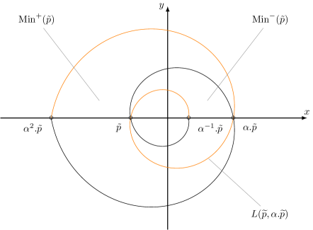
Furthermore, each photon becomes a logarithmic spiral contained in a -dimensional linear subspace of . The lightcone at a point is the revolution of any photon through around the axis connecting and . The complement of is a disjoint union of Minkowski patches, comprising the lifts of , where . The connected components are permuted by . Figure 1 shows a 2-dimensional cross-section of a light cone and a photon in it. The Minkowski patches are the regions bounded between successive loops. Two distinguished Minkowski patches adjacent to are labeled and ; these have a causal interpretation, which is given in the next section. A reference for this material is [1, Sec 4.3].
2.2.3. Causal Geometry of
A reference for some of the basic material on causality is [16, Chs 1–2]. Recall that a causal tangent vector is timelike or null, and a causal curve is one with causal velocity. A time-orientation of a Lorentzian manifold is given by a timelike vector field, and a simply connected Lorentzian manifold is always time-orientable. A causal tangent vector is future-pointing, respectively past-pointing, if its inner product with the time-orienting vector field is negative, respectively positive, and similarly for a causal curve. A piecewise smooth curve is called timelike, lightlike, or causal, respectively, if the velocity vectors, including the velocity from above and below at break points, are of the corresponding type; moreover, at the break points both velocity vectors must have the same time orientation—that is, all velocity vectors along the curve are future-pointing or all are past-pointing.
Definition 2.7.
For a time-orientable Lorentzian manifold, let .
-
(1)
chronologically precedes (often denoted ) if there is a future-directed timelike curve from to .
-
(2)
causally precedes (often denoted ) if there is a future-directed causal curve from to .
-
(3)
is causal if .
If but , we write .
Under the conformal equivalence
a time-orientation is given by the vector field . The map preserves time-orientation; thus is time-orientable, although it is not orientable (see [1, §4.2]). It is also causal (in fact, it is globally hyperbolic). For future reference, a natural choice of coordinate on gives, in homogeneous coordinates
| (2) |
Definition 2.8.
Let . The causal future set and future set are defined as
The causal past set and the past set are defined analogously.
The future and past sets of a point in have the following identifications in .
Lemma 2.9.
Let . Then the causal past and future can be expressed as
and the past and the future as
where denotes the standard Riemannian distance on .
The proof is left to the reader.
Remark 2.10.
An immediate consequence of the above lemma is that always causally precedes .
The causal future, respectively past, sets are the closure of the future, respectively past, sets. Note that given a point , its future set and its past set are not complementary; however,
Lemma 2.11.
For any point ,
Proof.
For , the distinguished Minkowski patch is the Minkowski patch containing in its closure and in the future of , while is the Minkowski patch containing in its closure, the points of which are not causally related to . We will take as definition the following, and verify a little later that these project to a Minkowski patch in as previously defined.
Definition 2.12.
For ,
-
(1)
,
-
(2)
.
The following relation follows immediately from Definition 2.12.
Proposition 2.13.
For any ,
For two points and such that for some , we define the following subsets, contained in :
The boundaries of the Minkowski patches are the following subsets of .
Corollary 2.14.
For any ,
Proof.
This proves the equality for ; the second follows from this one and Corollary 2.13. ∎
For a fixed and given any , there is such that
Strict inequality in the first case corresponds to , while strict inequality in the second case corresponds to . Equality corresponds to or , respectively. Thus is the disjoint union over of the Minkowski patches with . The first union and are each -invariant. It follows that the projection is the complement of in , which is the Minkowski patch . The projection of also equals .
2.3. Unipotent dynamics on
2.3.1. The maximal unipotent subgroup
The maximal unipotent subgroup of is the unipotent radical of the minimal parabolic subgroup. (These groups are of course unique only up to conjugacy in .) The latter subgroup is the stabilizer of an isotropic flag of ; the unipotent is the subgroup of the stabilizer of an isotropic flag which moreover acts trivially on each subquotient of the flag. For the quadratic form and the isotropic flag
the maximal unipotent subgroup is upper-triangular. It will be denoted . This group is simply connected, and is contained in . As is not in , it projects isomorphically to its image in , which we will also denote by .
Recall that denotes the conformal group of , for which we may also write . (Note that for , so is a two-fold quotient of the universal cover of .) Denote by the quotient. As this is a -covering on the identity components. We will denote by the full lift and by the identity component; the latter group is also isomorphic to , as is simply connected.
The isotropic flag stabilized by corresponds to the chain of subspaces
where is the photon obtained from the projectivization of . The -action on is the projective parabolic flow fixing . The -action on corresponds under the geometric isomorphism to the lift of this one-parameter subgroup to .
Because it stabilizes the complementary light cone, acts conformally on the Minkowski patch . By the Liouville Theorem 2.1, this action is faithful. The conformal group of is the similarity group . For , we denote by the image under the homomorphism . The image is a unipotent subgroup of , stabilizing the isotropic flag for the quadratic form . We denote by the -component of , so that acts on by the affine transformation . Note that is a 1-cocycle for the representation of on via .
2.3.2. The -flow
The maximal unipotent subgroup has one-dimensional center that corresponds to a translation by the isotropic vector on . We will refer to the -action of on as the -flow. In homogeneous coordinates on , it is
| (3) |
The lift to acting on will be denoted by as well. We will denote the corresponding vector fields on and by . In homogeneous coordinates on it is . Using the time orientation from (2), the inner product , vanishing exactly on . Thus is future-pointing on and .
Each point of tends under to a point of the fixed set as . The limit point is given by the projection from §2.2.1. As a consequence, we have the following description, for :
Similarly, the fixed set in of is and points of tend under to a point of as . Each Minkowski patch in can be written as a set of points converging to a particular segment of under the -flow. For any , denote , and similarly for .
Proposition 2.15.
For any
Proof.
From Corollary 2.14, we know that
For , let and . Let
and let be the -preimage of in . Since for all , we have
Thus . Note that the path for is future-pointing, as is future-pointing. If the two limits were equal, the result would be a closed causal loop, violating causality of (see §2.2.3). Moreover, the forward limit must be in the future of the backward limit, from which we conclude
On the other hand, every point of is the forward and backward limit of a point of under . As commutes with , every is for some for some ; also every is for some for some . By the inclusions proved in the previous paragraph, necessarily , and
The desired identity for now follows from Corollary 2.13. ∎
We now define . Let with .
This map is a submersion onto lifting .
2.3.3. An iterative technique for establishing completeness
The following is a general technique for showing that the developing map is a diffeomorphism onto eligible subsets of the model space . The basic version appears for affine manifolds with unipotent holonomy in the proof of completeness of [8, Thm 6.8] and our proof idea is derived from theirs.
Proposition 2.16.
Let be a developing pair for a -structure on a closed manifold , with holonomy image . Let be a connected, -invariant regular submanifold, with a -invariant foliation . Let be a connected component of . Assume is a closed set.
-
(1)
Suppose there are complete vector fields , such that, for all ,
-
•
is locally projectable modulo
-
•
If the image is -saturated, then is invariant by the flow along every .
-
•
-
(2)
Let be a connected, regular submanifold saturated by and by the flows along , such that
-
•
at all , the projections mod of form a frame of the local leaf space
-
•
on
Denote by the pulled-back foliation of , and let be a connected component of . If maps each leaf of in diffeomorphically to its image, then is a covering map onto .
-
•
A vector field is locally projectable modulo a foliation if every point has a foliated neighborhood with local leaf space such that for the projection , the push-foward is well-defined.
Proof.
Begin with the assumptions of (1). The first step is to build vector fields on corresponding to . Denote by the group of deck transformations of . The saturation is a union of closed connected components, so its projection to is closed, as is the component . For any , there is a neighborhood and a diffeomorphism from to a neighborhood . Let be a finite cover of by such neighborhoods, and define vector fields by pulling back from to , for each . Let be a partition of unity subordinate to and define . Let be the lift of to for each ; it is complete.
By the assumption of -invariance of , the pulled-back foliation descends to . For any , by the -invariance of mod , on the overlap of with some , the vector fields modulo the foliation. For the lifted vector fields , by construction, for any with neighborhood mapping diffeomorphically under to , the push-forward for all . In particular, the are projectable modulo .
We proceed to prove (1). Let for , and let for some . Consider for arbitrary a path , . Let and let for , which is defined because is complete. Let .
Now let where equivalence means belonging to the same leaf of . By construction . Suppose that with . By continuity of , , and , the leaves
so
Then is closed.
For , let be a sufficiently small transversal so that the -holonomy is defined on . Denote by the projection from a small neighborhood of to . Then is well-defined, by projectability. Shrinking if necessary, is also defined. These projected vector fields are equal, because modulo wherever both are defined. The projection , where defined, is the integral curve through of this vector field. Now let , a transversal to through . Here is defined, and , where defined, is its integral curve through . Because pushes forward to , it follows that . Then on a small interval of time around where these projections are both defined, . Thus is open. We conclude , so . By the hypothesis that is -saturated, , as desired.
Now let and be as in (2). Given , let be a foliated neighborhood with projection to the local leaf space. The hypotheses imply that after possibly shrinking , there is such that the map
is a diffeomorphism. Let be the image of . For a point of the leaf space, denote by the corresponding leaf. Let where . Given , denote by the composition .
Given , let denote the composition on . Given , reduce if necessary so that the map
is a diffeomorphism from to the local leaf space of a foliated neighborhood of . We will assume that is the full image of this map. Then maps bijectively via onto . Indeed, suppose and map under to the same point in . By equivariance of with respect to the flows and the foliations, that would mean . Then because the s commute modulo . Since , necessarily . Thus injectivity is proved. Surjectivity follows from equivariance of , as well.
For , define , where is the -leaf of in . By assumption, these map diffeomorphically to their images under for all . Thus maps bijectively, and hence diffeomorphically, to under .
Finally, suppose that for , there is . Then , where is the local leaf space of . By construction, there exist unique such that and each belong to this leaf. Then is in the same leaf as . Then is in the same leaf as . As , the first point is in , and the two points have the same projection under . By the assumption on , it follows that . But then and are in the same leaf, which implies they are equal because leaves map diffeomorphically under . Therefore the open sets are disjoint for distinct .
We conclude that is a covering from onto its image in . The image is open. If there were , then by the framing assumption of (2) it would be connected by a finite sequence of flows along and segments in leaves of to a point of . But then by the flow-invariance of and the assumption on along the foliations, would also be in the image . We conclude is a covering map of onto , as desired. ∎
3. The developing image contains .
Recall the -invariant flag
Our first case is when the image of contains . We prove in this case that the -structure on is complete—that is, is a diffeomorphism.
Theorem 3.1.
If the image of contains , then up to a finite covering, is the quotient of by a free, properly discontinuous -action that leaves invariant. More precisely, is finitely covered by where and .
The first step of the proof deals with the developing map vis-a-vis ; recall is connected. The following proposition serves for this case as well as the second case in the next section. Thus there is no special assumption on at this stage.
Proposition 3.2.
Any connected component of is mapped by diffeomorphically onto its image. In particular,
-
(1)
if , then maps diffeomorphically onto .
-
(2)
if , then maps diffeomorphically onto a connected component of , where .
Proof.
The restriction of to is the parabolic flow with unique fixed point —see §2.3.1. Denote the corresponding vector field on , and its lift to , by . The lift to vanishes precisely at the points and has no periodic points in each connected component of .
By Proposition 2.6, restricted to is a complete vector field on , and on in particular; moreover, the image is invariant by the flow along . The flow-invariant subsets of are subsets of and unions of components of .
In case (2) of this proposition, is one component of , which we will call . Such a component is parametrized by the flow along of any point in it. As intertwines the two corresponding flows, it follows in this case that maps diffeomorphically onto , as desired.
In case (1), observe that the saturation of by the deck transformations of is a union of connected components of the closed set , and therefore is also closed. Then is a closed photon, which inherits from the -structure on a -structure. Of course, the latter structure also has unipotent holonomy. From the classification of one-dimensional , -manifolds—see [12] or [9, §5.5]—the structure on is complete. The developing map of this structure is a diffeomorphism to , which is embedded into as —see §2.2.2. This developing map is the restriction of to , so we conclude that maps diffeomorphically onto . ∎
Completeness will extend from to all of with the help of the -flow. By Proposition 2.6, is a complete vector field on and the image of is -saturated. Denote by the corresponding flow on . The following lemma is proved using only the equivariance and local diffeomorphism properties of . The interval in the statement need not map diffeomorphically onto its image.
Lemma 3.3.
Let be open and connected. Then the set
is open in . The same holds for the analogously defined set .
Proof.
Let with , and let . The developing map intertwines the - and -flows. Because exists, it is mapped under to by continuity. By assumption, , so this latter limit can be expressed as . Choose connected neighborhoods and such that maps diffeomorphically to ; shrink them if necessary to ensure that .
Choose connected neighborhoods and such that maps diffeomorphically to , and let
which is again an open neighborhood of . Let .
Consider , and let . As converges uniformly on compact sets to , there are and a connected open containing and with for all . We can choose large enough that . Connectedness of implies that for all . Now is connected and open, so for any ,
Since exists and belongs to , it now follows via equivariance that exists and belongs to . As was an arbitrary point of , we conclude that , which completes the proof for . The proof for is completely analogous. ∎
Adding the assumption that maps diffeomorphically onto its image brings us to the key step for proving completeness.
Proposition 3.4.
Let be open and connected and be a connected component of . If maps to diffeomorphically, then the sets
each map diffeomorphically onto the sets
Proof.
The proof here is for and ; the other case is proved mutatis mutandis.
Let with , . As exists, it maps under to , for . Suppose that . Then by equivariance
By our assumption, this implies . Now let be a neighborhood of mapping diffeomorphically under to its image, which we will denote . Let be such that . By equivariance, . But then which implies . Therefore is injective in restriction to .
Next let , with . Let be the -preimage of . Let be a neighborhood of mapping diffeomorphically to , a neighborhood of . Let such that for all . Let . Then and .
Now restricted to the open set is a bijective local diffeomorphism onto , hence a diffeomorphism onto . ∎
We are ready to assemble the proof of Theorem 3.1. Assume that is in the image of . Let be a connected component of . By Proposition 3.2 (2), maps diffeomorphically onto . Let and . Proposition 3.4 above says that maps diffeomorphically under to . Since , the codimension of is at least two, so is path connected. Lemma 2.4 applies to and , to give that maps diffeomorphically to and equals . Any other component of would give disjoint from yet equal to —a contradiction. Therefore , so . Finally, is a bijective local diffeomorphism, so maps diffeomorphically onto . Completeness is proved.
To analyze the holonomy, recall that is a complete -manifold. The restricton to of the covering group action on is conjugated by to the action of on , for some . On the other hand, this restriction to is faithful, so . Since we assume that the holonomy projected to belongs to , it follows that with and .
4. The developing image does not contain but does meet
We continue to the second case of our classification. This case does not have an analogue in the conformal Riemannian setting.
4.1. The developing image
Write , and let be a connected component of meeting the image of . Let be a connected component of . By Proposition 3.2 (2), maps diffeomorphically under onto . The latter set is of the form
for some , which we will assume to be .
Let be the stabilizer of in the group of deck transformations of . As is homeomorphic to , so is . Proposition 2.5 gives that is closed; then , a connected component of this set, is also closed. Thus .
Let be the connected component containing . Note that . Let be a connected component of . The following proposition establishes completeness of between and . It is not assumed that meets ; part (2) of the proposition will be used for case 3, in §5 below.
Proposition 4.1.
Assume that . Let be a connected component of and . Let be a connected component of . Then maps diffeomorphically to its image, which equals
-
(1)
if .
-
(2)
if
Proof.
The submanifold is a connected component of , so it is closed in . On the other hand, is a regular submanifold. The holonomy subgroup leaves invariant, as does all of . The -orbit of is a union of connected components of . Thus can also be considered a connected component of the inverse image of the -invariant regular submanifold .
Let be the foliation of by photons. It is invariant by (and extends to a -invariant foliation of ). We have seen just above that if meets then any connected component of in maps diffeomorphically to under . On any photon in , the -flow acts simply transitively—this can be seen from the formula (3) for the -flow, taking and . By Proposition 2.6, is a complete vector field on . It follows that for any photon of , each component of is mapped diffeomorphically by to . We conclude that maps leaves of in diffeomorphically to leaves of in , where is the pulled-back foliation by photons on .
Next we define vector fields on . They will be lifted from . Denote by the foliation by photons on . Consider the map given in homogeneous coordinates by
| (4) |
It is an injective immersion onto . Let for . As is projectable under , and maps the fibers diffeomorphically to the photons of , it follows that is projectable modulo for all . The -action on preserves the image of and the foliation . The conjugated -action on descends to the -action by translations on , and thus centralizes modulo the -factor, for all . The -action on thus centralizes each modulo .
Let , a conformally embedded copy of , corresponding in homogeneous coordinates on to the locus where . In the affine chart on where , a routine calculation using (4) gives . In the affine chart where , the expression is
which tends to as . The origin of this affine chart corresponds to . The conclusion is that extends by to . Now lift the resulting vector fields on to ; we will continue to denote these by , for .
The vector fields are each projectable and -invariant modulo , thus they are -invariant (and -invariant when equivariantly extended to ) modulo . We are now in a position to apply Proposition 2.16. The image is invariant by the flow along for all , which means that it meets every leaf of . In case (1) or (2), maps onto the claimed set. In case (2), the vector fields form a framing of the local leaf space at every point of , so part (2) of Proposition 2.16 applies to give that is a covering map, which means it is a diffeomorphism.
In case (1), we take in Proposition 2.16 (2). It gives that any connected component of maps by a covering map onto , therefore by a diffeomorphism. By the following lemma, there is only one such component. Then is a bijective local diffeomorphism on , so it maps diffeomorphically to , as desired. ∎
Lemma 4.2.
For and as in Proposition 4.1 case (1), is connected.
Proof.
Let be a connected component of . Consider as in Lemma 3.3. Since maps diffeomorphically under to , Proposition 3.4 gives that maps diffeomorphically to , respectively. By Proposition 2.15, these are , respectively. By Corollary 2.14, the boundaries of these sets in are and , respectively.
For , let be a neighborhood mapping diffeomorphically to its image under , which will be denoted . Now
By shrinking to ensure that is connected, we may arrange that
Thus is open in . Since it is also closed and is connected, it follows that . The analogous argument implies .
Now suppose . Then meets and meets only the Minkowski patches ; by Proposition 3.4, . Now is a local diffeomorphism between the open sets
Any component of maps diffeomorphically to , as seen in the proof of Proposition 4.1. Then the open subset maps diffeomorphically onto the target above. Therefore by Proposition 2.4. ∎
With Proposition 4.1 and the arguments of the preceding proof, we have also established:
Proposition 4.3.
Let and be as in case (1) of Proposition 4.1. Then
-
•
is open and is mapped diffeomorphically by onto .
-
•
is connected.
The following complete description of will conclude this subsection.
Proposition 4.4.
The set in the conclusion of Proposition 4.3 equals , and . The developing map is a diffeomorphism of onto , and the holonomy image is a subgroup of isomorphic to .
Proof.
Assume to the contrary that there is . Then . From Corollary 2.14 the boundaries of are contained in the three punctured light cone components for . One of these, , equals and is in the interior of . Therefore
By construction, is contained in the stabilizer of ; the latter intersects in . Thus is also contained in the stabilizer of and for all . Without loss of generality, we assume . Let be a nonempty connected component. Proposition 4.1 implies that maps diffeomorphically onto or under . By the usual argument with Proposition 2.5, the stabilizer in of acts cocompactly. On the other hand, this stabilizer maps isomorphically to . It is then impossible that . Therefore necessarily maps diffeomorphically under onto .
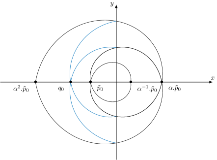
Now develops diffeomorphically to . The latter set is the closure of in by Corollary 2.14. We will show that does not act properly on this set. Let be the origin of the Minkowski patch , and let . Since any two lightcones in intersect, the images intersect for any . The closure does not meet —it is easily seen from the Minkowski chart in §2.2.1 that —so is a compact subset of contained in . Thus is compact, and intersects its image under any . Because acts properly by deck transformations on , this is a contradiction. See Figure 2. The conclusions of the proposition now follow. ∎
4.2. Determination of holonomy, conclusion of classification
It is established that ; moreover, is generated by an element of acting freely, properly discontinuously, and cocompactly on , , and . We first establish necessary conditions on this generator, which we will call .
Proposition 4.5.
Let be the generator of the holonomy image under the assumptions of this section, and let . Let be the affine decomposition as in Section 2.3.1. Then is nontrivial modulo . Moreover, if , then is timelike.
Proof.
The restriction of to corresponds in the affine representation to the projection of modulo , and this must be nontrivial.
Next suppose that , and let . Let be the chart on given in (4). In this chart, the action of is by
where the scalar product on is the one with quadratic form . The lines
describe the full null cone of except for the line . We have already established that is not orthogonal to . Then will pointwise fix some photon of unless is not orthogonal to any line in . Since must act freely on , we conclude that is timelike. ∎
Lemma 4.6.
Let , and suppose there is that satisfies
-
(1)
,
-
(2)
and .
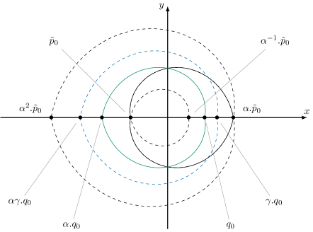
Then acts on with precompact fundamental domain given by
See Figure 3 for a diagram of this fundamental domain in .
Proof.
We first prove that the union covers the entirety of . From Lemma 2.11,
As both and preserve time orientation,
which gives
It thus follows that
From (2),
.
Since succeeds each ,
For any set , the future and past satisfy [16, Prop 2.11]. Taking , we obtain the reverse containment and conclude
From (2), . For all , , so for all . By the argument with [16, Prop 2.11] as above, we obtain
We can finally conclude that
which by definition equals .
It remains to show for all . Let be given, which we may assume is positive. From (1), it follows that
By Lemma 2.11, we can also express
The desired disjointness now follows. ∎
Proposition 4.7.
Proof.
First suppose that is a translation by a timelike vector . Considering if necessary, we may assume is future-pointing. Then evidently, for the origin of , we have .
Under the Minkowski embedding in , the limit is . Thus . By Corollary 2.14, both limits belong to . On the other hand, the forward limit is in the future of , so could only equal . The backward limit is in the past of . Lemma 2.11 gives that the complement of is —that is, points of are not causally related to . Then . The sufficient condition (2) is thus verified for the case that .
We now consider , satisfying and . For , the linear part acts by
Replacing by if necessary, we can arrange that . In the Minkowski patch of ,
| (5) |
To evaluate the causal asymptotics of this sequence, recall given by (2). Under the inverse of the Minkowski chart (see §2.2.1), it pushes forward to
which has negative inner product with everywhere in . We may use this latter vector field for time orientation on (see [15, Lem 5.29]). Since it is a constant vector field, a vector will be in the future light cone of the origin exactly when .
Now
Replacing by for some sufficiently large , we obtain , and condition (1) of Lemma 4.6 is verified in this case.
The dominant term in (5) is the coefficient of . Under the Minkowski embedding, the limit points of are in (here ). On the other hand, acts nontrivially on with unique attracting fixed point . Therefore . For , the formula (5) becomes
Here again the -component is dominant, and the same argument as for gives . Then we conclude as in the translation case that . Sufficient condition (2) of Lemma 4.6 is verified. ∎
This case is now finished; the main results are summarized below. The examples with a timelike translation were previously discovered by C. Frances in his dissertation [4, Sec 7.6.3].
Theorem 4.8.
If the image of does not contain but does meet , then, up to composition with a conformal transformation, is a diffeomorphism onto . The holonomy image for satisfying the necessary and sufficient conditions in Proposition 4.5. The manifold is diffeomorphic to .
5. The developing image does not meet the photon but does meet the lightcone .
In this case, the unipotence of the holonomy image leads, with the help of Proposition 2.16, to being a diffeomorphism of onto . Using, among other things, the algebraic hull of the holonomy, we prove that there are no examples in odd dimensions. In even dimensions, we find a family of Heisenberg fiber bundles over the circle.
5.1. Development and holonomy for light cone components
Let . The space consists of infinitely many connected components . By case (2) of Proposition 4.1, maps each connected component of diffeomorphically to for each .
We now choose components and . Denote by the stabilizer of in the group of deck transformations. Because is a diffeomorphism to its image, the holonomy restricts to an isomorphism of with its image, which will be denoted . The latter lies in the stabilizer of , hence, under our assumptions, in . The restriction of to is faithful, thus so is the restriction of to .
Lemma 5.1.
The action of on is cocompact. The cohomological dimension equals .
Proof.
The hypersurface is a connected component of the -inverse image of the closed, -invariant set . Then is closed by our standard arguments with Proposition 2.5. The second statement follows from . ∎
Now we will focus on . Note that is a diffeomorphism from to . This means that is an isomorphism from to .
For , recall the affine decomposition of §2.3.1, and that the projection is abelian.
Lemma 5.2.
The linear projection spans the abelian Lie group . The image is discrete only if is nontrivial.
Proof.
The leaf space for the foliation of by photons is identified with the round sphere , on which the -action factors through the projection and is conformal. The quotient of by the photon foliation is thus identified with the punctured round sphere. Under stereographic projection, this leaf space is conformal to . The action of is by translations. (This is the same action as appears in the proof of Proposition 4.1.)
By Lemma 5.1, is cocompact on . Since is -equivariantly diffeomorphic via to , it follows that acts cocompactly on , and thus on the leaf space of the invariant foliation by photons. A group of translations of is cocompact if and only if it spans . Thus spans .
If is trivial, then maps isomorphically to its image in . Thus is a free abelian group in this case. On the other hand, by Lemma 5.1, and because , it has cohomological dimension . Thus . It follows that is not discrete in this case. ∎
Lemma 5.3.
The intersection is generated by a single, possibly trivial, null translation in the center of . If it is nontrivial, then is discrete.
Proof.
Denote . It is a free abelian group; let its rank be . The quotient is also a free abelian group, of rank at least by Lemma 5.2. On the other hand, . We conclude that .
Of course is normal in . If is nontrivial, it is isomorphic to . The conjugation action of on is moreover unipotent; therefore, it is trivial, and is central in . Because spans , must be contained in the common fixed space of in , which is a one-dimensional isotropic subspace. It acts on by .
Finally, if , then the rank of the free abelian group is at most by Lemma 5.1. Again, because this image spans , its rank is and it is discrete in this case. ∎
Corollary 5.4.
If or , then is abelian.
Proof.
If , then , which is abelian. If and is nontrivial, then by Lemma 5.3, is a central extension of by , which is necessarily abelian. ∎
5.2. Development and holonomy for Minkowski patches
Let be the foliation of by the fibers of (see 2.3.2). Because the developing image is contained in and is invariant by , it pulls back to a foliation of by degenerate hypersurfaces, invariant by the group of deck transformations, which we will denote . Each leaf of is a connected component of the -preimage of a leaf in . One of these leaves is , which is already known to map diffeomorphically under to . We now prove the same property for every leaf of the foliation.
Proposition 5.5.
For the foliation of pulled back by from , each leaf in maps diffeomorphically to a leaf of .
Proof.
We begin by defining vector fields on . In the Minkowksi chart , they are coordinate vector fields of
The two Minkowski charts and cover —their complement is the projectivization of . The second Minkowski chart is
The change of coordinates is
For , the push forward by the change of coordinates is
These vector fields thus extend to smooth vector fields on .
Note that corresponds to , and that here, the s are all tangent to the foliation of the lightcone by photons. Then evidently in restriction to , the -action leaves invariant modulo for all . Also, as they do not depend on , the s are all projectable modulo on . In the coordinates on , the foliation by photons is the linear foliation tangent to , and is trivial on , which means it fixes modulo for all . As the are all constant in these coordinates, they are projectable modulo inside , too. Lastly, note that the s commute on .
Now lift to , keeping the same notation for them. They are -invariant modulo the foliation by photons and projectable modulo . The -flow is simply transitive on each photon of . As always, since commutes with , it pulls back to a complete flow on by Proposition 2.6. Thus for the subfoliation by photons, each leaf maps diffeomorphically under to its image in .
As previously noted, every leaf of mapping into maps diffeomorphically to a connected component of . Therefore, we will consider for some for the remainder of the proof.
Part (1) of Proposition 2.16 gives that the image of is invariant by the flow along any . For , the orbit of under these flows, saturated by , is the full leaf . For , the form a framing modulo in restriction to . Then Proposition 2.16 part (2), for , gives that the leaf mapping onto maps by a covering. As , this is a diffeomorphism. ∎
Proposition 5.6.
Suppose that the image of intersects for some . Then an open subset maps diffeomorphically under to .
Proof.
By Proposition 5.5, the image of is -saturated; moreover, maps -leaves diffeomorphically to -leaves. To define a transverse vector field on , we reprise the Minkowski charts and on as in the proof of that proposition.
Under the change of coordinates,
Then the coordinate vector field on extends by to , the set corresponding to in . We obtain a well-defined vector field on . As is constant in the chart and elsewhere, it is projectable modulo . As acts trivially on , and vanishes on the complement of , it is -invariant modulo .
Now lift to , where it will still be denoted . It is -invariant and projectable modulo . Take . It is saturated by and by the flow along ; moreover, is nonzero modulo everywhere in . Then for any connected component of , Proposition 2.16 says that maps diffeomorphically onto . ∎
A neighborhood of intersects at least one such . The holonomy subgroup lies in and preserves each Minkowski patch in . Thus leaves invariant the open sets corresponding to Minkowski patches neighboring in . Let one such be . It is mapped diffeomorphically under to . The -action on is thus conjugate to the -action on . We now consider the latter action in detail, and recall that . We will write the group and not distinguish from for this discussion.
The leaf space of in is diffeomorphic via to . Fix for the remainder of this section an identification with , with the quadratic form of §2.2.1. Denote by the homomorphism sending an element of to its action on this leaf space. The leaf space can also be identified with , on which is translation by , the translational component of transverse to .
Proposition 5.7.
If , then . On the leaf space of in , the action of is trivial.
For , the commutator is easily seen to be
| (6) |
The identification of with can be made explicitly as follows: in our coordinates on , elements act by
| (7) |
for a unique . Denote .
Proof.
The aim is to prove that for all , the translational component . Since the linear part preserves each leaf of in , it will then follow that preserves each leaf. The corresponding statement about will follow from Proposition 5.6.
Let , and let correspond to and as above. The commutator given by (6) belongs to . The latter subgroup acts on by a group of translations in the direction of by Lemma 5.3. Thus
for all . If for one , the component , then by Lemma 5.3, and must be linearly dependent with for all . If , then the latter conclusion contradicts Lemma 5.2. ∎
The action of on is affine and properly discontinous. Viewing as a subgroup of the affine group of , there is a connected algebraic hull which acts properly on and contains as a cocompact lattice (see [7, Thm 1.4]). In fact, acts freely on as well [7, Lem 1.9]. By the proposition above, is contained in if , so it acts freely and properly on each hyperplane in the foliation in this case.
Lemma 5.8.
For the algebraic hull of in , there are nontrivial translations in , that is, .
Proof.
Suppose that . By Lemma 5.1 and because , the group . Thus the algebraic hull , and it intersects the kernel of nontrivially.
If , then evidently also has nontrivial intersection. ∎
We establish some basic structural features of . Since spans by Lemma 5.2, the linear projection of the algebraic hull equals . For , the translational component is given by a 1-cocycle ; by Proposition 5.7, this cocycle has values in . Because acts trivially on , composing with projection to yields a homomorphism. Recall the identification of with via from (7). Define
Proposition 5.9.
Assume that and let be the algebraic hull, with associated as above. If has a real eigenvalue, then does not act properly on ; more precisely, if is a real eigenvalue, then acts with noncompact stabilizers on the affine hyperplane defined by .
Proof.
Let be an eigenvector of with eigenvalue . Because projects onto , there is an element with . By definition, . Given , equation (7) says
Thus , and the 1-parameter subgroup of containing , act trivially modulo on the affine hyperplane defined by . The translations belong to , as well, by Lemma 5.8. Therefore any vector in this hyperplane has a noncompact stabilizer, proving nonproperness. ∎
5.3. The global picture
As above, is the algebraic hull of in .
Proposition 5.10.
Suppose that . Then does not act properly on .
From this proposition we conclude there are no -dimensional examples for which meets but not .
Proof.
Let be a connected component of in the image of , as above. Let have in its closure, so that by Proposition 5.6, there is mapping diffeomorphically to .
Let . Note that, under the Minkowski chart the closure in is a photon not meeting . Now consider the lift ; the closure in is compact, contained in . It is therefore the diffeomorphic image of a compact photon in .
Fix a generater of and write with for each . We can write mod . Then, whenever , we can take to obtain
Because projects onto , there is an unbounded set of with . On the other hand, by Lemmas 5.8 and 5.3, the translations by are in . Therefore, there is an unbounded subset of for which . As is a lattice in , there are infinitely many and a compact subset such that for . Then there are a compact subset and infinitely many such that . ∎
Proposition 5.11.
The developing map is a diffeomorphism of with .
This lemma will be used in the proof.
Lemma 5.12.
The developing map induces a local homeomorphism between the leaf space and the corresponding leaf space in . In fact, the induced map on leaf spaces is a diffeomorphism to its image, which is an open interval in .
Proof.
Let and let be a neighborhood of mapping diffeomorphically under to its image in . Shrink as necessary so that admits a transversal submanifold to through mapping diffeomorphically to its image in the leaf space of .
Let be the corresponding transversal to the foliation in , so that restricted to is a diffeomorphism to . Let be the image of in the leaf space of . The map sending leaves of to leaves of is well-defined because intertwines the two foliations. The inverse map is the composition of two differomorphisms with a quotient map; it is evidently continuous.
It remains to verify that the map is continuous. An open subset is diffeomorphic to a relatively open subset . There is moreover an -saturated open subset such that . Now
The projection of the set on the left-hand side is the inverse image of in . The expression on the right-hand side exhibits it as an open subset of .
Now that we have shown that the map on leaf spaces is a local homeomorphism, it follows that the leaf space in is a one-dimensional manifold, and the map between leaf spaces is a local diffeomorphism. The image in the leaf space of is open and connected, thus an open interval. The leaf space in is therefore diffeomorphic to and maps diffeomorphically to its image. ∎
We now prove Proposition 5.11.
Proof.
The image of the developing map is an open, contiguous union of Minkowski charts and their interstitial light cone components . By Lemma 5.12, factors through a map on leaf spaces which is a diffeomorphism to an open interval . The fibers of the composition are the leaves of , which is thus a simple foliation of . By Proposition 5.5, it follows that is diffeomorphic to and maps diffeomorphically under to its image. Therefore maps isomorphically under to its image .
It remains to show the image of is all of . Suppose that is a finite interval in . Then it contains for finitely many . A finite index subgroup of stabilizes each light cone component; let one of them be . For , the group is isomorphic to and has finite index in . Then by Lemma 5.1. This contradicts acting properly discontinuously and cocompactly on . Therefore is infinite.
Denote by the homomorphism given by restriction to , which also corresponds to the action on the leaf space of . As acts cocompactly on , it contains elements with nontrivial translation number. The invariance of by such an element implies that . ∎
By Proposition 5.10 we may assume , and then Proposition 5.7 says that , where is as defined in the proof above. The image projects under to the unipotent subgroup fixing , which we will denote . As with , this group has a lift to , so . But cannot intersect : the inverse image in of this intersection would stabilize and would thus be contained in , a contradiction. Therefore is generated by a single element acting properly discontinuously and cocompactly on the leaf space of .
Proposition 5.13.
The holonomy image is generated by and another element of the form , where and normalizes . The projection of to belongs to .
Proof.
It remains only to verify the last claim. Equation (6) gives for ,
The result is in with image under equal . The translational part is
which must equal because . Therefore and .
∎
We summarize the results obtained thus far, under the standing assumptions of this section: The developing map is a diffeomorphism to . The dimension of is . The group has a normal subgroup which maps isomorphically under to its image , which has algebraic hull contained in . Any element of is of the form with and . The algebraic hull of contains the center of and is encoded by a linear endomorphism with no real eigenvalues; in particular for some .
5.4. Heisenberg examples and conclusion
The first result of this section underlies the construction of actions whenever the conditions summarized at the end of the previous section are fulfilled. Then we give the classification for this case.
Proposition 5.14.
Let . Let and let be any element with these eigenvalues. Define to be the connected group generated by
Then acts simply transitively on and on for each .
Proof.
Fix and let where . An element acts by
The result is congruent to only if . By the construction of , the latter condition implies and . Thus the stabilizer in of is trivial. Moreover, for each , the set of spans . The action is simply transitive on .
Recall the parametrization of by of (4). Assuming , the action of maps to
The stablizer of has which means . The stabilizer also has , which means is trivial. It is also evident from the above formula that acts transitively on . ∎
From such an -action, we can easily construct geometries on compact satisfying the assumptions of this section.
Theorem 5.15.
If the image of does not meet but does meet , then is even, and is a diffeomorphism onto . For a nilpotent group as in Proposition 5.14 and a lattice , the holonomy is a nilpotent extension , for some and . In this case, is a nilmanifold of degree at most 3, which fibers over with degree-2 nilmanifold fibers.
Proof.
Let be as defined in §5.1, and let be its algebraic hull in . By Proposition 5.10 . By Proposition 5.7 and Lemmas 5.3 and 5.8 , and , so is determined by an endomorphism of as in §5.2. By Proposition 5.9, has no real eigenvalues, which forces , hence , to be even. We conclude that must be as in Proposition 5.14. It is of nilpotence degree 2.
Proposition 5.11 establishes that is a diffeomorphism onto .
The conclusions of Proposition 5.14 allow us to identify the fibration with a principal -bundle. The image of under the isomorphism will also be denoted . Then is a principal -bundle over .
By construction, is a cocompact lattice in . Let be the image of in . As observed after Proposition 5.11, is generated by an element of the form with and in the normalizer in of ; we may assume . Since splits as a product , there is a splitting . The remaining conclusions follow. ∎
6. Conclusion of classification, including essential examples
The last case in our classfication reduces to a class of manifolds that have been well studied.
Theorem 6.1.
If the image of does not meet , then is a complete -manifold. It is for a nilpotent group of degree at most 3 acting simply transitively on , and a cocompact lattice in .
Proof.
The hypothesis implies that maps into . The -action on here is by affine isometries. As , the pair defines an -structure on . Y. Carrière proved that any such structure on a closed manifold is complete—that is, is a diffeomorphism of onto [2].
Now is an isomorphism to , and . The algebraic hull of is a unipotent subgroup of acting simply transitively on . These were classified by F. Grünewald and G. Margulis in [11, Thm 1.8]. They are all nilpotent groups of degree at most . ∎
6.1. Proof of Theorem 1.4.
Recall that the flow is in the center of . That means it always descends to a conformal flow on , which we will denote , in our setting of unipotent holonomy.
Proposition 6.2.
For as in cases (1) or (2) of Theorem 1.2, the conformal flow is essential. For as in cases (3) or (4), it is inessential.
Proof.
In cases (1) or (2), let be a nontrivial, open interval contained in the image of . The inverse image is open. For any volume on , the volume while . In fact, for any compact set with nonempty interior, . Now tends uniformly to a subset of ast , which implies that does not preserve any volume on . In particular, it does not preserve a -invariant volume lifted from . Therefore does not preserve any volume on , so it must be essential.
In case (3), is not abelian. The lattice having as algebraic hull is therefore not abelian, so its commutator subgroup intersects nontrivially. The -flow on factors through the quotient by this intersection, which is . It is therefore not essential.
Finally, acts on by a lightlike translation, which is isometric. In case (4), , and is isometric on , so the flow is isometric on . ∎
In light of Theorem 1.2 and Proposition 6.2, it remains only to prove that as in cases (3) or (4) does not admit an essential conformal flow.
In case (4), any conformal flow on lifts on to . Any non-isometric flow in this group is a homothety. But a homothety cannot descend to a closed manifold. Thus there is no essential conformal flow in this case.
In case (3), any conformal flow of that descends to belongs to the identity component of the normalizer of and to the stabilizer of . Because is discrete, such a flow belongs in fact to , the identity component of the centralizer of . Now , so , as is the Zariski closure of . We descend to and analyze the centralizer of intersect the stabilizer of in . Let .
The stabilizer of in corresponds to the stabilizer of , and has Levi decomposition
The kernel of intersect is precisely . It contains , and their centers coincide; we will denote this central subgroup by . The usual generators of are . These can be chosen with for all , so that we can view as a basis for and as a basis for . The isomorphism of (7) corresponds in this basis to for all .
Since must act trivially on , its projection to has image in . Now we consider the centralizer in of . The latter representation is , where each is a copy of the standard representation. Recall that is the graph of an isomorphism with no real eigenvalues, as in Proposition 5.14. If is a noncompact 1-parameter subgroup centralizing , it leaves invariant the graph of , which we will denote . Since , each is of dimension at most 1. Let denote the eigenvectors of on , possibly equal; denote by the corresponding vectors in for each . Invariance implies that equals the sum of its intersections with . Any nontrivial intersection is generated by for some , which would correspond to a real eigenvalue of , a contradiction. We conclude that the centralizer of in is compact.
References
- [1] T. Barbot, V. Charette, T. Drumm, W. Goldman, and K. Melnick, A primer on the -Einstein universe, Recent developments in pseudo-Riemannian geometry: Proceedings of the special semester “Geometry of pseudo-Riemannian manifolds with applications to physics,” September - December, 2005 (Zürich) (D. Alekseevsky and H. Baum, eds.), ESI Lect. Math. Phys., Erwin Schrödinger Insitute, Eur. Math. Soc., 2008, pp. 179–229.
- [2] Y. Carrière, Autour de la conjecture de L. Markus sur les variétés affines, Invent. Math. 95 (1989), no. 3, 615–628.
- [3] C. Daly, Closed affine manifolds with an invariant line, Ph.D. thesis, University of Maryland, College Park, 2021, unpublished thesis.
- [4] C. Frances, Géométrie et dynamique lorentziennes conformes, Ph.D. thesis, École Normale Supérieure de Lyon, 2002.
- [5] by same author, About pseudo-Riemannian Lichnerowicz conjecture, Transform. Groups 20 (2015), no. 4, 1015–1022.
- [6] C. Frances and K. Melnick, The Lorentzian Lichnerowicz Conjecture for real-analytic, three-dimensional manifolds, J. für die Reine und Angew. Math. (2023), no. 803, 183–218.
- [7] D. Fried and W. Goldman, Three-dimensional affine crystallographic groups, Advances in Math. 47 (1983), no. 1, 1–49.
- [8] D. Fried, W. Goldman, and M. Hirsch, Affine manifolds with nilpotent holonomy., Comment. Math. Helv. 56 (1981), 487–523.
- [9] W. Goldman, Geometric structures on manifolds, Grad. Studies in Math., vol. 227, Amer. Math. Society, 2022.
- [10] W.M. Goldman, Conformally flat manifolds with nilpotent holonomy and the uniformization problem for 3-manifolds, Trans. Amer. Math. Soc. 278 (1983), no. 2, 573–583.
- [11] F. Grünewald and G. Margulis, Transitive and quasitransitive actions of affine groups preserving a generalized lorentz-structure, J. Geom. Phys. 5 (1988), no. 4, 493–531.
- [12] N. H. Kuiper, Locally projective spaces of dimension one, Michigan Math. J. 2 (1953), no. 2, 95 – 97.
- [13] J. Lelong-Ferrand, Transformations conformes et quasiconformes des variétés riemanniennes; application à la démonstration d’une conjecture de A. Lichnerowicz, Acad. Roy. Belg. Cl. Sci. Mém. 39 (1971), no. 5, 5–44.
- [14] M. Obata, The conjectures on conformal transformations of Riemannian manifolds, J. Differential Geom. 6 (1971), 247–258.
- [15] B. O’Neill, Semi-riemannian geometry with applications to relativity, Academic Press, San Diego, 1983.
- [16] R. Penrose, Techniques of differential topology in relativity, CBMS-NSF Regional Conference Series in Applied Mathematics, SIAM, 1972.
- [17] R.W. Sharpe, Differential geometry : Cartan’s generalization of Klein’s Erlangen program, Springer, New York, 1996.
| Rachel Lee | Karin Melnick | |
| Department of Mathematics | Department of Mathematics | |
| 4176 Campus Drive | 6 avenue de la Fonte | |
| University of Maryland | University of Luxembourg | |
| College Park, MD 20742 | L-4364 Esch-sur-Alzette | |
| USA | Luxembourg | |
| rachel.youcis.lee@gmail.com | karin.melnick@uni.lu |