TFWT: Tabular Feature Weighting with Transformer
Abstract
In this paper, we propose a novel feature weighting method to address the limitation of existing feature processing methods for tabular data. Typically the existing methods assume equal importance across all samples and features in one dataset. This simplified processing methods overlook the unique contributions of each feature, and thus may miss important feature information. As a result, it leads to suboptimal performance in complex datasets with rich features. To address this problem, we introduce Tabular Feature Weighting with Transformer, a novel feature weighting approach for tabular data. Our method adopts Transformer to capture complex feature dependencies and contextually assign appropriate weights to discrete and continuous features. Besides, we employ a reinforcement learning strategy to further fine-tune the weighting process. Our extensive experimental results across various real-world datasets and diverse downstream tasks show the effectiveness of TFWT and highlight the potential for enhancing feature weighting in tabular data analysis.
1 Introduction
Extracting feature information from data is one of the most crucial tasks in machine learning, especially for classification and prediction tasks Bishop (1995). Different features play varied roles in data representation and pattern recognition, thus directly impacting the model’s learning efficiency and prediction accuracy. Effective feature engineering can enhance a model’s ability to handle complex data significantly and help capture critical information in the data.
In feature engineering, a traditional and common assumption is that each feature in a dataset is equally essential. Treating all features equally important does simplify the process, but it ignores the fact that each feature contributes uniquely to the downstream task Daszykowski et al. (2007). Some features with rich information may significantly impact the model outcome, while others may contribute less or even introduce noise and mislead the model García et al. (2015). Treating all features with equal weight may dilute the information of important features and cause less important features to over-influence the model, thus diminishing the overall effectiveness of information extraction. Feature weighting is a technique that assigns weights to each feature in the dataset. The main goal of feature weighting is to optimize the feature space by assigning weights to each feature according to feature importance, thus enhancing the model performance. Feature weighting methods can be categorized based on learning strategies and weighting methods. Supervised feature weighting uses actual data labels to determine the weights of features Chen and Hao (2017a); Niño-Adan et al. (2020); Wang et al. (2022). Unsupervised feature weighting utilizes the intrinsic characteristics of the dataset to assign weight without relying on label information Zhang et al. (2018).
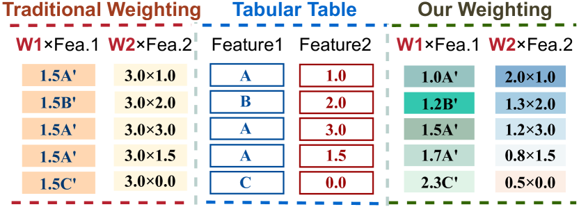
Feature weighting can also be classified based on feature types or feature information. Weighting by feature types focuses on the inherent properties of features, like discreteness or continuity. This approach is often influenced by data structure Zhou et al. (2021); Xue et al. (2023); Hashemzadeh et al. (2019); Cardie and Howe (1997); Lee et al. (2011). Conversely, weighting by feature information emphasizes the informational content of features. It assesses the importance of features based on their correlation and contribution to the predictive model, typically using statistical measures or machine learning algorithms Kang et al. (2019); Liu et al. (2004); Druck et al. (2008); Zhu et al. (2023a); Liu et al. (2019). However, these methods do not effectively capture the complex relationships between features and cause risks like overfitting, local optimality, and noise sensitivity. Moreover, as illustrated in Figure 1, these methods assign the same weight to every sample (row) of each feature, rather than assigning personalized weights to different samples.
In addressing the limitations of traditional feature weighting methods, we adopt a new approach based on the Transformer model. One core feature of the Transformer is its self-attention mechanism Vaswani et al. (2017); Radford et al. (2019); Luong et al. (2015); Zhou et al. (2023); Siriwardhana et al. (2020); Hashemzadeh et al. (2019). This mechanism can effectively identify complex dependencies and interactions among data features. In feature weighting, the self-attention mechanism assigns attention weights by considering the relevance and contribution of features, enabling the model to learn and adapt to specific dataset patterns during the training process. Thus, our Transformer-based approach can assign higher weights to features that significantly influence the model output. In this way, the model can focus on the most critical information. With self-attention, the Transformer can effectively capture the contextual information and inter-feature relationships within the tabular data.
The Transformer also employs a multi-head attention mechanism operated with several self-attention components operating in parallel. Each attention head focuses on different aspects of the dataset, and captures diverse patterns and dependencies. Thus the model can understand the feature relationships from multiple perspectives. This application of multi-head attention significantly enhances the model’s capability in determining feature weights. Thus, by integrating self-attention and multi-head attention mechanisms, our Transformer-based method effectively identifies and assigns feature weights. It adapts to various data patterns and complicated relationships among features.
To further stabilize and enhance this weighting structure, we need an effective fine-tuning method. Adopting reinforcement learning Schulman et al. (2017); Fan et al. (2020) for fine-tuning is a common strategy Ziegler et al. (2019); Fickinger et al. (2021); Ouyang et al. (2022); Zhu et al. (2020). Notably, the Proximal Policy Optimization (PPO) network Schulman et al. (2017) has the advantage of stability and efficiency in fine-tuning by enhancing policies while ensuring stable updates Zhu et al. (2023b). Specifically, the PPO network fits the task of reducing information redundancy within the data. In this scenario, information redundancy refers to the presence of repetitive or irrelevant information. Redundant features lead to possible overfitting in training. By reducing redundancy, the data becomes more concise and focused on the most informative features. By minimizing redundancy, learning becomes more stable and focused, which helps to decrease classification variance.
In summary, we propose a novel feature weighting method aiming to tackle several challenges: first, how to generate appropriate weights of features; second, how to evaluate the effectiveness of feature weights; and finally, how to fine-tune the feature weights according to the feedback from downstream tasks. Hence, we introduce a Transformer-enhanced feature weighting framework in response to the challenges outlined. This framework leverages the strength of the Transformer architecture to assign weights to features by capturing intricate contextual relationships among these features. We evaluate the effectiveness of feature weighting by the improvement of downstream task’s performance. Further, we adopt a reinforcement learning strategy to fine-tune the output and reduce information variance. This adjustment enhances the model’s stability and reliability.
Our contributions are summarized as follows:
-
•
We propose a novel feature weighting method for tabular data based on Transformer called TFWT. This new method can capture the dependencies between features with Transformer’s attention mechanism to assign and adjust weights for features according to the feedback of downstream tasks.
-
•
We propose a fine-tuning method for the weighting process to further enhance the performance. This fine-tuning method adopts a reinforcement learning strategy, reducing the data information redundancy and classification variance.
-
•
We conduct extensive experiments and show that TFWT achieves significant performance improvements under varying datasets and downstream tasks, comparing with raw classifiers and baseline models. The experiments also show the effectiveness of fine-tuning process in reducing redundancy.
2 Related Work
2.1 Feature Weighting
Feature weighting, vital for enhancing machine learning, includes several approaches Chen and Guo (2015); Chen and Hao (2017b); Chowdhury et al. (2023); Wang et al. (2004); Yeung and Wang (2002). Liu et al. (2004), Druck et al. (2008), and Raghavan et al. (2006) explored feedback integration, model constraints, and active learning enhancement. Wang et al. (2013) proposed an active SVM method for image retrieval. Techniques like weighted bootstrapping Barbe and Bertail (1995), chi-squared tests, TabTransformer Huang et al. (2020), and cost-sensitive learning adjust weights through feature changes. These methods have limitations like overfitting or ignoring interactions. Our study focuses on adaptable weight distribution and improvement through feedback.
2.2 Transformer
The Transformer architecture, introduced by Vaswani et al. (2017), has revolutionized many fields including natural language processing. Instead of relying on recurrence like its predecessors, it utilizes self-attention mechanisms to capture dependencies regardless of their distance in the input data. This innovation has led to several breakthroughs in various tasks. For instance, BERT model Devlin et al. (2018); Clark et al. (2019), built upon the Transformer, set new records in multiple NLP benchmarks. Later, Radford et al. (2019) extended these ideas with GPT-2 and GPT-3 Brown et al. (2020), demonstrating impressive language generation capabilities. Concurrently, Raffel et al. (2020) proposed a unified text-to-text framework for NLP transfer learning, achieving state-of-the-art results across multiple tasks.
3 Methodology
3.1 Problem Formulation
We consider the problem setting of classification. Let be a dataset with features and samples. We define the feature matrix . We use to denote the -th feature, where is the value of -th sample on the -th feature. is the label vector. Without loss of generality, we assume the first features to be discrete, and the remaining features to be continuous.
In defining a weighting matrix , each of whose elements corresponds to the elements of the feature matrix . This weighting matrix is applied element-wisely to to produce a weighted matrix , where denotes the Hadamard product. In the weighting problem, we aim to find an optimized , so that can improve the downstream tasks’ performance when substituting the original feature matrix in predicting .
3.2 Framework
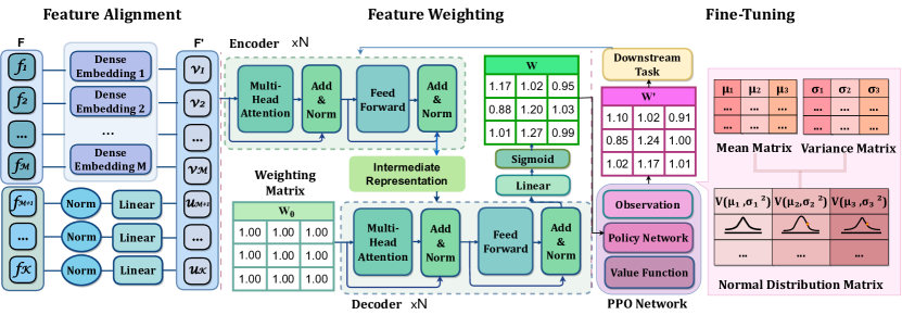
We propose TFWT, a Tabular Feature Weighting with Transformer method for tabular data. We aim to improve downstream tasks’ performance by effectively incorporating the attention mechanism to capture the relations and interactions between features. To achieve this goal, we design a Transformer-based feature weighting pipeline with a fine-tuning strategy. As Figure 2 shows, our method consists of three components: In the Feature Alignment, we align different types of original features so that they are in the same space. In the Feature Weighting, we encode the feature matrix to get its embedding via Transformer encoders, and then decode the embedding into feature weights. In the Fine-Tuning, we design a reinforcement learning strategy to fine-tune the feature weights based on feedback from downstream tasks.
3.3 Feature Alignment
To effectively extract tabular data’s features while maintaining a streamlined computation, we convert both discrete and continuous features into numerical vectors.
Discrete Feature Alignment. We first encode the discrete features into numerical values. The encoded numerical values are then passed to a dense embedding layer, transforming them into vectors for subsequent processes. For each discrete feature (), the encoded vector is:
| (1) |
Continuous Feature Alignment. We normalize all the continuous features with mean of 0 and variance of 1. We then design a linear layer to align their length with discrete features. For each continuous feature (), the encoded vector is:
| (2) |
where and are the mean and standard deviation of the -th feature, respectively. Then the aligned feature matrix is formed by concatenating these vectors:
| (3) |
3.4 Feature Weighting
Given aligned feature matrix , we aim to explore the relationships between features and assign proper feature weights.
Data Encoding. To enhance the model’s understanding and extract latent patterns and relations from the data, we put into the encoders with a multi-head self-attention mechanism. This mechanism processes the embedded feature matrix by projecting it into query (Q), key (K), and value (V) spaces.
The encoder then applies the self-attention mechanism to capture varying feature relations in the feature matrix and assigns distinct attention weights to them. Assuming is the dimensionality of the key vectors, the attention mechanism is formulated as:
| (4) |
where , , and , , , are parameter matrices.
In our method, we adopt the multi-head attention mechanism, where the results of each head are concatenated and linearly transformed. Assuming is an output projection matrix and is the feature representation:
| (5) |
| (6) |
| (7) |
where , , and are weights for query, key, and value. Through this process, we obtain the feature representation that captures feature relationships. Specifically, is obtained by passing the input feature matrix through multiple layers of the encoder, where each layer applies self-attention and residual connection-enhanced feedforward networks.
Weight Decoding. In this process, we aim to decode a weighting matrix from the embedding . This decoding process iteratively updates until the downstream task’s performance is satisfied. We initialize the by setting all its elements as 1. This is to ensure all features receive equal importance at the beginning. In each decoding layer, we do cross-attention on and by:
| (8) |
where , , and , , , are parameter matrices.
By adopting a cross-attention mechanism, we generate a contextual representation that captures various relationships and dependencies in the feature matrix. After several weight decoding layers, we get an updated weighting matrix :
| (9) |
We finally use the the weighting matrix to derive a weighted feature matrix by its Hadamard product with the original feature matrix : . With this weighted feature matrix, we reorganize the feature space and make features optimized for the downstream task. is then used to substitute in the downstream tasks.
3.5 Fine-Tuning
In the fine-tuning process, our primary goal is to adopt a reinforcement learning strategy to adjust the weighting matrix . This adjustment aims to reduce information redundancy of , thereby reducing the variance during training.
Weighting Matrix Refinement. We begin by evaluating the redundancy, denoted as , using mutual information as defined by Shannon (1948). is calculated as follows:
| (10) |
In this formula, represents the feature matrix, with and being the -th and -th features, respectively. The function measures the mutual information between these two features. We further define to represent the change in redundancy, where , is the redundancy of the feature matrix after fine-tuning.
Next, we process the input weighting matrix through a RL model. In this paper, we adopt a Proximal Policy Optimization (PPO) as our RL model, which comprises one actor network and one critic network Schulman et al. (2017). While the actor network focuses on determining the actions to take, the critic evaluates how good those actions are, based on the expected rewards. In this content, an action is defined as the output of the PPO network, which is an adjusted weighting matrix . The state is the weighting matrix and the reward is the change of redundancy .
Specifically, the actor network processes to produce mean and variance values. These values are then used to form a probability distribution matrix , which consists of Gaussian distributions, represented as:
| (11) |
| (12) |
Here, indicates the weight distribution of , the -th element of the -th feature, with and being the mean and variance, respectively. Here we form with each element sampled from the probability distribution .
Actor Network Update. After refining the weighting matrix, we update the feature matrix as , and subsequently calculate the information redundancy of . Based on the observed change of redundancy , we adjust the mean and variance within the probability distribution, following the equations:
| (13) |
| (14) |
where is the parameter of the actor network, is the learning rate, is the objective function to maximize, is the gradient of the objective function with respect to the mean and variance, is the number of state-action pairs in the training, is the policy, and is the reward of state-action pair . To ensure a stable fine-tuning process, we implement a clipping mechanism for the updated means. Specifically, we adopt each mean using the formula: . This clipping process is crucial for as it prevents excessive deviations from the current weight , thereby maintaining the stability and reducing the variance during downstream training.
Critic Network Update. After the update of actor network, we continue to adjust the critic network with the reward. We design the critic network to provide an estimate of the advantage function . This advantage function represents the expected future advantages under the state and action . We design the function to change the policy gradually based on the current state, so that the policy after adjustment is not too biased from the previous policy . We adopt the clipping mechanism with a parameter as well as the advantage function in the loss function:
| (15) |
By minimizing , we continuously optimize the feature matrix to obtain stable and enhanced performance.
3.6 Training of TFWT
As Algorithm 1 shows, we first align original features by Eq.1 and Eq.2. Then, we encode the aligned feature matrix into an embedding and decode it into a weighting matrix . This encoding-decoding process is accomplished by a designated Transformer. In this way, we get a weighted feature matrix . To further fine-tune , we adopt PPO as a reinforcement learning model to reduce the redundancy of . The fine-tuned is sampled from the actor network of PPO. The PPO networks are trained by the interaction data from the sampling process. The cross-entropy loss derived from the downstream machine learning model is used to update the parameters of the encoders and decoders in the Transformer.
4 Experiments
In this section, we present three experiments that validate the strength of our method. First, we demonstrate that our method significantly enhances the performance on various downstream tasks without fine-tuning. Second, we demonstrate the advantages of our TFWT method over the baseline methods. Finally, we demonstrate the effectiveness of fine-tuning comparing with non-fine-tuning version of TFWT in reducing the variance performance metrics. Overall, the results consistently demonstrate the superior performance of our method.
| Metrics | Model | RF | LR | NB | KNN | MLP | |||||||||||||||
|---|---|---|---|---|---|---|---|---|---|---|---|---|---|---|---|---|---|---|---|---|---|
| Acc | AM | OS | MA | SD | AM | OS | MA | SD | AM | OS | MA | SD | AM | OS | MA | SD | AM | OS | MA | SD | |
| Raw | 0.620 | 0.850 | 0.812 | 0.702 | 0.660 | 0.873 | 0.787 | 0.724 | 0.600 | 0.780 | 0.731 | 0.679 | 0.567 | 0.843 | 0.808 | 0.674 | 0.687 | 0.868 | 0.812 | 0.716 | |
| USP | 0.613 | 0.863 | 0.817 | 0.682 | 0.640 | 0.869 | 0.751 | 0.710 | 0.587 | 0.766 | 0.744 | 0.692 | 0.560 | 0.858 | 0.815 | 0.662 | 0.653 | 0.869 | 0.819 | 0.720 | |
| Lasso | 0.627 | 0.860 | 0.822 | 0.707 | 0.680 | 0.860 | 0.799 | 0.724 | 0.607 | 0.802 | 0.738 | 0.669 | 0.533 | 0.852 | 0.816 | 0.679 | 0.693 | 0.878 | 0.821 | 0.719 | |
| WB | 0.613 | 0.868 | 0.823 | 0.690 | 0.667 | 0.861 | 0.790 | 0.710 | 0.633 | 0.786 | 0.742 | 0.692 | 0.567 | 0.857 | 0.822 | 0.664 | 0.707 | 0.869 | 0.821 | 0.722 | |
| TabT | 0.620 | 0.882 | 0.851 | 0.708 | 0.660 | 0.879 | 0.797 | 0.725 | 0.600 | 0.817 | 0.741 | 0.688 | 0.567 | 0.869 | 0.822 | 0.678 | 0.687 | 0.878 | 0.851 | 0.723 | |
| TFWT | 0.640 | 0.895 | 0.860 | 0.733 | 0.713 | 0.903 | 0.805 | 0.727 | 0.627 | 0.829 | 0.752 | 0.694 | 0.587 | 0.884 | 0.833 | 0.685 | 0.727 | 0.894 | 0.874 | 0.739 | |
| Prec | AM | OS | MA | SD | AM | OS | MA | SD | AM | OS | MA | SD | AM | OS | MA | SD | AM | OS | MA | SD | |
| Raw | 0.622 | 0.727 | 0.827 | 0.706 | 0.657 | 0.789 | 0.777 | 0.701 | 0.613 | 0.659 | 0.739 | 0.681 | 0.537 | 0.707 | 0.838 | 0.656 | 0.687 | 0.788 | 0.822 | 0.716 | |
| USP | 0.629 | 0.714 | 0.801 | 0.706 | 0.634 | 0.761 | 0.754 | 0.708 | 0.583 | 0.649 | 0.716 | 0.694 | 0.633 | 0.786 | 0.828 | 0.683 | 0.664 | 0.766 | 0.810 | 0.736 | |
| Lasso | 0.624 | 0.747 | 0.816 | 0.694 | 0.684 | 0.771 | 0.789 | 0.724 | 0.607 | 0.680 | 0.732 | 0.670 | 0.544 | 0.851 | 0.831 | 0.679 | 0.689 | 0.806 | 0.820 | 0.725 | |
| WB | 0.614 | 0.765 | 0.876 | 0.753 | 0.670 | 0.775 | 0.788 | 0.710 | 0.619 | 0.662 | 0.728 | 0.699 | 0.557 | 0.790 | 0.840 | 0.660 | 0.707 | 0.793 | 0.835 | 0.722 | |
| TabT | 0.622 | 0.788 | 0.860 | 0.710 | 0.657 | 0.799 | 0.786 | 0.725 | 0.613 | 0.687 | 0.742 | 0.688 | 0.537 | 0.787 | 0.821 | 0.688 | 0.687 | 0.812 | 0.840 | 0.731 | |
| TFWT | 0.637 | 0.856 | 0.842 | 0.742 | 0.710 | 0.803 | 0.789 | 0.727 | 0.627 | 0.694 | 0.769 | 0.696 | 0.557 | 0.801 | 0.845 | 0.707 | 0.730 | 0.825 | 0.871 | 0.739 | |
| Rec | AM | OS | MA | SD | AM | OS | MA | SD | AM | OS | MA | SD | AM | OS | MA | SD | AM | OS | MA | SD | |
| Raw | 0.622 | 0.722 | 0.761 | 0.702 | 0.655 | 0.658 | 0.741 | 0.701 | 0.602 | 0.729 | 0.661 | 0.680 | 0.705 | 0.631 | 0.749 | 0.636 | 0.687 | 0.662 | 0.772 | 0.716 | |
| USP | 0.582 | 0.714 | 0.818 | 0.616 | 0.633 | 0.781 | 0.779 | 0.709 | 0.579 | 0.721 | 0.666 | 0.681 | 0.524 | 0.609 | 0.761 | 0.659 | 0.651 | 0.668 | 0.793 | 0.719 | |
| Lasso | 0.622 | 0.700 | 0.789 | 0.736 | 0.678 | 0.633 | 0.748 | 0.724 | 0.603 | 0.771 | 0.661 | 0.659 | 0.510 | 0.812 | 0.758 | 0.679 | 0.690 | 0.700 | 0.780 | 0.718 | |
| WB | 0.614 | 0.715 | 0.748 | 0.562 | 0.667 | 0.638 | 0.747 | 0.705 | 0.616 | 0.727 | 0.649 | 0.672 | 0.546 | 0.602 | 0.754 | 0.670 | 0.710 | 0.665 | 0.769 | 0.722 | |
| TabT | 0.622 | 0.715 | 0.821 | 0.708 | 0.655 | 0.655 | 0.755 | 0.725 | 0.602 | 0.777 | 0.668 | 0.688 | 0.705 | 0.668 | 0.785 | 0.678 | 0.687 | 0.635 | 0.839 | 0.723 | |
| TFWT | 0.641 | 0.688 | 0.847 | 0.732 | 0.710 | 0.741 | 0.761 | 0.727 | 0.634 | 0.750 | 0.658 | 0.693 | 0.782 | 0.626 | 0.774 | 0.685 | 0.730 | 0.701 | 0.840 | 0.739 | |
| F1 | AM | OS | MA | SD | AM | OS | MA | SD | AM | OS | MA | SD | AM | OS | MA | SD | AM | OS | MA | SD | |
| Raw | 0.620 | 0.725 | 0.777 | 0.701 | 0.656 | 0.694 | 0.752 | 0.701 | 0.591 | 0.676 | 0.666 | 0.679 | 0.432 | 0.654 | 0.766 | 0.624 | 0.687 | 0.697 | 0.785 | 0.716 | |
| USP | 0.556 | 0.734 | 0.807 | 0.658 | 0.633 | 0.770 | 0.746 | 0.709 | 0.578 | 0.664 | 0.677 | 0.687 | 0.418 | 0.637 | 0.779 | 0.650 | 0.646 | 0.699 | 0.800 | 0.714 | |
| Lasso | 0.622 | 0.719 | 0.798 | 0.714 | 0.676 | 0.665 | 0.761 | 0.724 | 0.602 | 0.703 | 0.669 | 0.664 | 0.403 | 0.826 | 0.776 | 0.679 | 0.690 | 0.735 | 0.793 | 0.717 | |
| WB | 0.613 | 0.736 | 0.772 | 0.644 | 0.666 | 0.671 | 0.758 | 0.708 | 0.617 | 0.680 | 0.658 | 0.685 | 0.532 | 0.629 | 0.776 | 0.665 | 0.705 | 0.700 | 0.787 | 0.722 | |
| TabT | 0.620 | 0.743 | 0.834 | 0.707 | 0.656 | 0.693 | 0.765 | 0.725 | 0.591 | 0.712 | 0.677 | 0.688 | 0.432 | 0.703 | 0.797 | 0.674 | 0.687 | 0.673 | 0.839 | 0.720 | |
| TFWT | 0.636 | 0.735 | 0.844 | 0.730 | 0.710 | 0.767 | 0.771 | 0.727 | 0.621 | 0.715 | 0.667 | 0.692 | 0.463 | 0.664 | 0.794 | 0.676 | 0.730 | 0.742 | 0.852 | 0.728 | |
| Datasets | Samples | Features | Class |
|---|---|---|---|
| AM | 1,500 | 10,000 | 2 |
| OS | 12,330 | 17 | 2 |
| MA | 19,020 | 10 | 2 |
| SD | 991,346 | 23 | 2 |
4.1 Experimental Settings
Datasets. We evaluate the proposed method with four real-world datasets:
-
•
Amazon Commerce Reviews Set (AM) Liu (2011) from UCI consists of customer reviews from the Amazon Commerce website. Its purpose is to classify the identities of authors of reviews by analyzing textual patterns. We have randomly divided its labels into two groups, each containing labels, transforming it into a balanced binary classification task.
-
•
Online Shoppers Purchasing Intention Dataset (OS) Sakar and Kastro (2018) from UCI features multivariate data types including integer and real values. Its purpose is to classify shoppers’ purchasing intentions and predict purchases.
-
•
MAGIC Gamma Telescope Dataset (MA) Bock (2007) from UCI reflects the simulation of high energy gamma particles registration in a gamma telescope. Its purpose is to classify the primary gammas from cosmic rays.
-
•
Smoking and Drinking Dataset with body signal (SD) Her (2023) from Kaggle is collected from National Health Insurance Service in Korea. Its purpose is to classify “smoker” or “drinker”.
Downstream Tasks. We apply the proposed model across a diverse array of classification tasks, including Random Forests (RF), Logistic Regression (LR), Naive Bayes (NB), K-Nearest Neighbor (KNN) and Multilayer Perceptrons (MLP). We compare the performance outcomes in these tasks both with and without our method.
Baseline Models. To demonstrate the effectiveness of our method, We compare our TFWT method with four established baseline techniques, where the Least Absolute Shrinkage and Selection Operator and TabTransformer are used for feature preprocessing, and Weighted Bootstrapping and Undersampling handle sample weight preprocessing.
-
•
Undersampling (USP) reduces the majority class in a dataset to balance with the minority class, creating an even dataset. This method minimizes majority class bias in training. We set the undersampling ratio based on category frequency in our experiments.
-
•
Least Absolute Shrinkage and Selection Operator (LASSO) is a technique for feature selection and regularization, enhancing model accuracy and interpretability. It introduces a penalty proportional to the absolute values of coefficients, encouraging sparsity by driving some to zero. This process effectively selects crucial features, simplifying the model and reducing data dimensionality.
-
•
Weighted Bootstrapping (WB) Barbe and Bertail (1995) is a resampling technique assigning weights to each dataset instance, influencing their selection in the resampled dataset. It’s particularly useful for balancing underrepresented classes. In our experiments, weights are determined by class frequency.
-
•
TabTransformer (TabT) Huang et al. (2020) is a method designed for tabular data, inspired by Transformer technology from natural language processing. It specializes in transforming categorical features into embeddings, capturing complex relationships within the data. This approach enhances the performance of tabular data in downstream tasks. In our experiments, TabTransformer processes categorical features to create enriched representations, which are then integrated into our model.
Metrics. To evaluate our proposed method, we use the following metrics: Overall Accuracy (Acc) measures the proportion of true results (both true positives and true negatives) in the total dataset. Precision (Prec) reflects the ratio of true positive predictions to all positive predictions for each class. Recall (Rec), also known as sensitivity, reflects the ratio of true positive predictions to all actual positives for each class. F-Measure (F1) is the harmonic mean of precision and recall, providing a single score that balances both metrics.
Implementation Details. We implemented TFWT using PyTorch and Scikit-learn. The models were trained on NVIDIA A100. For each dataset, we randomly selected between and as training data. We initialized the hyperparameters for the baseline models following the guidelines in the corresponding papers, and carefully adjusted them to ensure optimal performance. The initial learning rate was set between and . For model regularization, the dropout rate was fixed at .
4.2 Experimental Results
Overall Performance. Table 1 illustrates that our TFWT method consistently surpasses baseline methods across a variety of metrics and datasets. For example, when focusing on MLP, TFWT attains an accuracy improvement ranging from to compared to raw downstream tasks, and from to improvement over the most competitive feature weight adjustment methods. Furthermore, when applying fine-tuning method, TFWT sees an additional accuracy increase from to , and a variance decline from to . Notably, our method also consistently outperforms the TabTransformer model, which also incorporates the Transformer for feature adjustment.
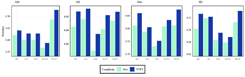
Enhancement over Raw Downstream Tasks. Our evaluation focuses on the improvement that TFWT method brings to various downstream tasks in terms of performance. To ensure a robust and reliable comparison, we execute each model configuration five times and calculate the average metrics. The comparative results, showcased in Figure 3 and Table 1, clearly demonstrate that TFWT consistently boosts performance across all four metrics in four datasets, particularly when applied to MLP. The significant improvement incorporated in the TFWT method enhances the performance of downstream tasks from multiple dimensions.
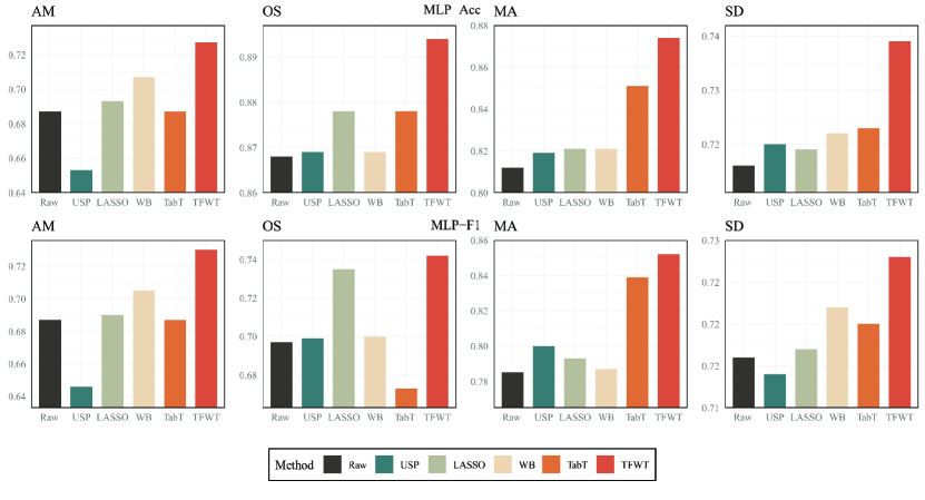
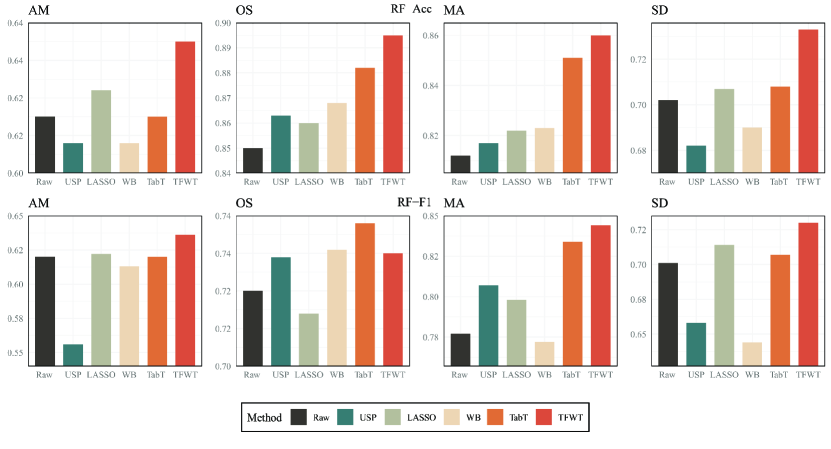
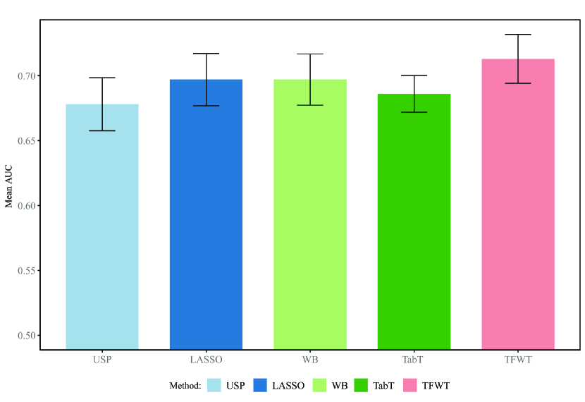
Superiority over Baseline Models. We examine the impacts of our TFWT approach and conduct comparative analyses against four baseline models across four performance metrics. Our primary metric of representation is overall accuracy, depicted in Figure 3. Our TFWT method consistently achieves the highest accuracy on all four datasets. Particularly noteworthy is the comparison with TabTransformer model. While TabTransformer also integrates a Transformer structure in the feature preprocess, TFWT demonstrates a marked superiority in accuracy and F1.
| Model Name | Mean AUC |
|---|---|
| USP | 0.678 0.025 |
| LASSO | 0.697 0.020 |
| WB | 0.686 0.014 |
| TabT | 0.697 0.020 |
| TFWT | 0.713 0.019 |
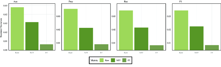
Superiority of Fine-Tuning Method. We further evaluate the advantages brought by our fine-tuning methodology. The refined results post fine-tuning not only match but in several instances surpass the outcomes obtained without fine-tuning, across all evaluated metrics. The key aspect is that the fine-tuned model demonstrates its superiority in the significant reduction of variance across these metrics. Taking Random Forests as a specific example, in a series of five repeated experiments, the variance in results after fine-tuning decreased by to across all four metrics compared with the non-fine-tuned TFWT model. Furthermore, the variance decreased by to compared with raw random forest.
5 Conclusion
In this study, we introduce TFWT, a weighting framework designed to automatically assign weights to features in tabular datasets to improve classification performance. Through this method, we utilize the attention mechanism of Transformers to capture dependencies between features to assign and adjust weights iteratively according to the feedback of downstream tasks. Moreover, we propose a fine-tuning strategy adopting reinforcement learning to refine the feature weights and to reduce information redundancy. Finally, we present extensive testing across various real-world datasets to validate the effectiveness of TFWT in a broad range of downstream tasks. The experimental results demonstrate that our method significantly outperforms the raw classifiers and baseline models.
6 Acknowledgements
This work was supported by the Strategic Priority Research Program of the Chinese Academy of Sciences XDB38030300, the National Key R&D Program of China under Grand No. 2021YFE0108400, the Natural Science Foundation of China under Grant No. 61836013, and Informatization Plan of Chinese Academy of Sciences (CAS-WX2023ZX01-11).
References
- Barbe and Bertail [1995] Philippe Barbe and Patrice Bertail. The weighted bootstrap, volume 98. Springer Science & Business Media, 1995.
- Bishop [1995] Christopher M Bishop. Neural networks for pattern recognition. Oxford university press, 1995.
- Bock [2007] R. Bock. MAGIC Gamma Telescope. UCI Machine Learning Repository, 2007.
- Brown et al. [2020] Tom Brown, Benjamin Mann, Nick Ryder, Melanie Subbiah, Jared D Kaplan, Prafulla Dhariwal, Arvind Neelakantan, Pranav Shyam, Girish Sastry, Amanda Askell, et al. Language models are few-shot learners. Advances in neural information processing systems, 33:1877–1901, 2020.
- Cardie and Howe [1997] Claire Cardie and Nicholas Howe. Improving minority class prediction using case-specific feature weights. 1997.
- Chen and Guo [2015] Lifei Chen and Gongde Guo. Nearest neighbor classification of categorical data by attributes weighting. Expert Systems with Applications, 42(6):3142–3149, 2015.
- Chen and Hao [2017a] Yingjun Chen and Yongtao Hao. A feature weighted support vector machine and k-nearest neighbor algorithm for stock market indices prediction. Expert Systems with Applications, 80:340–355, 2017.
- Chen and Hao [2017b] Yingjun Chen and Yongtao Hao. A feature weighted support vector machine and k-nearest neighbor algorithm for stock market indices prediction. Expert Systems with Applications, 80:340–355, 2017.
- Chowdhury et al. [2023] Stiphen Chowdhury, Na Helian, and Renato Cordeiro de Amorim. Feature weighting in dbscan using reverse nearest neighbours. Pattern Recognition, 137:109314, 2023.
- Clark et al. [2019] Kevin Clark, Urvashi Khandelwal, Omer Levy, and Christopher D Manning. What does bert look at? an analysis of bert’s attention. arXiv preprint arXiv:1906.04341, 2019.
- Daszykowski et al. [2007] Michal Daszykowski, Krzysztof Kaczmarek, Yvan Vander Heyden, and Beata Walczak. Robust statistics in data analysis—a review: Basic concepts. Chemometrics and intelligent laboratory systems, 85(2):203–219, 2007.
- Devlin et al. [2018] Jacob Devlin, Ming-Wei Chang, Kenton Lee, and Kristina Toutanova. Bert: Pre-training of deep bidirectional transformers for language understanding. arXiv preprint arXiv:1810.04805, 2018.
- Druck et al. [2008] Gregory Druck, Gideon Mann, and Andrew McCallum. Learning from labeled features using generalized expectation criteria. In Proceedings of the 31st annual international ACM SIGIR conference on Research and development in information retrieval, pages 595–602, 2008.
- Fan et al. [2020] Wei Fan, Kunpeng Liu, Hao Liu, Pengyang Wang, Yong Ge, and Yanjie Fu. Autofs: Automated feature selection via diversity-aware interactive reinforcement learning. In 2020 IEEE International Conference on Data Mining (ICDM), pages 1008–1013. IEEE, 2020.
- Fickinger et al. [2021] Arnaud Fickinger, Hengyuan Hu, Brandon Amos, Stuart Russell, and Noam Brown. Scalable online planning via reinforcement learning fine-tuning. Advances in Neural Information Processing Systems, 34:16951–16963, 2021.
- García et al. [2015] Salvador García, Julián Luengo, and Francisco Herrera. Data preprocessing in data mining, volume 72. Springer, 2015.
- Hashemzadeh et al. [2019] Mahdi Hashemzadeh, Amin Golzari Oskouei, and Nacer Farajzadeh. New fuzzy c-means clustering method based on feature-weight and cluster-weight learning. Applied Soft Computing, 78:324–345, 2019.
- Her [2023] Sooyoung Her. Smoking and drinking dataset. Kaggle, 2023.
- Huang et al. [2020] Xin Huang, Ashish Khetan, Milan Cvitkovic, and Zohar Karnin. Tabtransformer: Tabular data modeling using contextual embeddings. arXiv preprint arXiv:2012.06678, 2020.
- Kang et al. [2019] Bingyi Kang, Zhuang Liu, Xin Wang, Fisher Yu, Jiashi Feng, and Trevor Darrell. Few-shot object detection via feature reweighting. In Proceedings of the IEEE/CVF International Conference on Computer Vision, pages 8420–8429, 2019.
- Lee et al. [2011] Chang-Hwan Lee, Fernando Gutierrez, and Dejing Dou. Calculating feature weights in naive bayes with kullback-leibler measure. In 2011 IEEE 11th International Conference on data mining, pages 1146–1151. IEEE, 2011.
- Liu et al. [2004] Bing Liu, Xiaoli Li, Wee Sun Lee, and Philip S Yu. Text classification by labeling words. In Aaai, volume 4, pages 425–430, 2004.
- Liu et al. [2019] Kunpeng Liu, Yanjie Fu, Pengfei Wang, Le Wu, Rui Bo, and Xiaolin Li. Automating feature subspace exploration via multi-agent reinforcement learning. In Proceedings of the 25th ACM SIGKDD International Conference on Knowledge Discovery & Data Mining, pages 207–215, 2019.
- Liu [2011] Zhi Liu. Amazon Commerce reviews set. UCI Machine Learning Repository, 2011.
- Luong et al. [2015] Minh-Thang Luong, Hieu Pham, and Christopher D Manning. Effective approaches to attention-based neural machine translation. arXiv preprint arXiv:1508.04025, 2015.
- Niño-Adan et al. [2020] Iratxe Niño-Adan, Itziar Landa-Torres, Eva Portillo, and Diana Manjarres. Analysis and application of normalization methods with supervised feature weighting to improve k-means accuracy. In 14th International Conference on Soft Computing Models in Industrial and Environmental Applications (SOCO 2019) Seville, Spain, May 13–15, 2019, Proceedings 14, pages 14–24. Springer, 2020.
- Ouyang et al. [2022] Long Ouyang, Jeffrey Wu, Xu Jiang, Diogo Almeida, Carroll Wainwright, Pamela Mishkin, Chong Zhang, Sandhini Agarwal, Katarina Slama, Alex Ray, et al. Training language models to follow instructions with human feedback. Advances in Neural Information Processing Systems, 35:27730–27744, 2022.
- Radford et al. [2019] Alec Radford, Jeffrey Wu, Rewon Child, David Luan, Dario Amodei, Ilya Sutskever, et al. Language models are unsupervised multitask learners. OpenAI blog, 1(8):9, 2019.
- Raffel et al. [2020] Colin Raffel, Noam Shazeer, Adam Roberts, Katherine Lee, Sharan Narang, Michael Matena, Yanqi Zhou, Wei Li, and Peter J Liu. Exploring the limits of transfer learning with a unified text-to-text transformer. The Journal of Machine Learning Research, 21(1):5485–5551, 2020.
- Raghavan et al. [2006] Hema Raghavan, Omid Madani, and Rosie Jones. Active learning with feedback on features and instances. The Journal of Machine Learning Research, 7:1655–1686, 2006.
- Sakar and Kastro [2018] C. Sakar and Yomi Kastro. Online Shoppers Purchasing Intention Dataset. UCI Machine Learning Repository, 2018. DOI: https://doi.org/10.24432/C5F88Q.
- Schulman et al. [2017] John Schulman, Filip Wolski, Prafulla Dhariwal, Alec Radford, and Oleg Klimov. Proximal policy optimization algorithms. arXiv preprint arXiv:1707.06347, 2017.
- Shannon [1948] Claude Elwood Shannon. A mathematical theory of communication. The Bell system technical journal, 27(3):379–423, 1948.
- Siriwardhana et al. [2020] Shamane Siriwardhana, Tharindu Kaluarachchi, Mark Billinghurst, and Suranga Nanayakkara. Multimodal emotion recognition with transformer-based self supervised feature fusion. IEEE Access, 8:176274–176285, 2020.
- Vaswani et al. [2017] Ashish Vaswani, Noam Shazeer, Niki Parmar, Jakob Uszkoreit, Llion Jones, Aidan N Gomez, Łukasz Kaiser, and Illia Polosukhin. Attention is all you need. Advances in neural information processing systems, 30, 2017.
- Wang et al. [2004] Xizhao Wang, Yadong Wang, and Lijuan Wang. Improving fuzzy c-means clustering based on feature-weight learning. Pattern recognition letters, 25(10):1123–1132, 2004.
- Wang et al. [2013] Xiang-Yang Wang, Bei-Bei Zhang, and Hong-Ying Yang. Active svm-based relevance feedback using multiple classifiers ensemble and features reweighting. Engineering Applications of Artificial Intelligence, 26(1):368–381, 2013.
- Wang et al. [2022] LiMin Wang, XinHao Zhang, Kuo Li, and Shuai Zhang. Semi-supervised learning for k-dependence bayesian classifiers. Applied Intelligence, pages 1–19, 2022.
- Xue et al. [2023] Yu Xue, Chenyi Zhang, Ferrante Neri, Moncef Gabbouj, and Yong Zhang. An external attention-based feature ranker for large-scale feature selection. Knowledge-Based Systems, 281:111084, 2023.
- Yeung and Wang [2002] Daniel S. Yeung and XZ Wang. Improving performance of similarity-based clustering by feature weight learning. IEEE transactions on pattern analysis and machine intelligence, 24(4):556–561, 2002.
- Zhang et al. [2018] Guang-Yu Zhang, Chang-Dong Wang, Dong Huang, Wei-Shi Zheng, and Yu-Ren Zhou. Tw-co-k-means: Two-level weighted collaborative k-means for multi-view clustering. Knowledge-Based Systems, 150:127–138, 2018.
- Zhou et al. [2021] HongFang Zhou, JiaWei Zhang, YueQing Zhou, XiaoJie Guo, and YiMing Ma. A feature selection algorithm of decision tree based on feature weight. Expert Systems with Applications, 164:113842, 2021.
- Zhou et al. [2023] Wei Zhou, Peng Dou, Tao Su, Haifeng Hu, and Zhijie Zheng. Feature learning network with transformer for multi-label image classification. Pattern Recognition, 136:109203, 2023.
- Zhu et al. [2020] Yifan Zhu, Hao Lu, Ping Qiu, Kaize Shi, James Chambua, and Zhendong Niu. Heterogeneous teaching evaluation network based offline course recommendation with graph learning and tensor factorization. Neurocomputing, 415:84–95, 2020.
- Zhu et al. [2023a] Yifan Zhu, Fangpeng Cong, Dan Zhang, Wenwen Gong, Qika Lin, Wenzheng Feng, Yuxiao Dong, and Jie Tang. WinGNN: dynamic graph neural networks with random gradient aggregation window. In The 29th ACM SIGKDD Conference on Knowledge Discovery and Data Mining, KDD 2023. ACM, 2023.
- Zhu et al. [2023b] Yifan Zhu, Qika Lin, Hao Lu, Kaize Shi, Donglei Liu, James Chambua, Shanshan Wan, and Zhendong Niu. Recommending learning objects through attentive heterogeneous graph convolution and operation-aware neural network. IEEE Transactions on Knowledge and Data Engineering, 35(4):4178–4189, 2023.
- Ziegler et al. [2019] Daniel M Ziegler, Nisan Stiennon, Jeffrey Wu, Tom B Brown, Alec Radford, Dario Amodei, Paul Christiano, and Geoffrey Irving. Fine-tuning language models from human preferences. arXiv preprint arXiv:1909.08593, 2019.