SeNMo: A Self-Normalizing Deep Learning Model for Enhanced Multi-Omics Data Analysis in Oncology

Abstract

Multi-omics research has enhanced our understanding of cancer heterogeneity and progression. Investigating molecular data through multi-omics approaches is crucial for unraveling the complex biological mechanisms underlying cancer, thereby enabling more effective diagnosis, treatment, and prevention strategies. However, predicting patient outcomes through the integration of all available multi-omics data is still an under-study research direction. Here, we present SeNMo (Self-normalizing Network for Multi-omics), a deep neural network that has been trained on multi-omics data across 33 cancer types. SeNMo is particularly efficient in handling multi-omics data characterized by high-width (many features) and low-length (fewer samples) attributes. We trained SeNMo for the task of overall survival of patients using pan-cancer multi-omics data involving 33 cancer sites from the Genomics Data Commons (GDC). The training multi-omics data includes gene expression, DNA methylation, miRNA expression, DNA mutations, protein expression modalities, and clinical data. We evaluated the model’s performance in predicting patient’s overall survival using the concordance index (C-Index). SeNMo performed consistently well in the training regime, reflected by the validation C-Index of $0.76$ on GDC’s public data. In the testing regime, SeNMo performed with a C-Index of $0.758$ on a held-out test set. The model showed an average accuracy of $99.8\%$ on the task of classifying the primary cancer type on the pan-cancer test cohort. SeNMo proved to be a mini-foundation model for multi-omics oncology data because it demonstrated robust performance, and adaptability not only across molecular data types but also on the classification task of predicting the primary cancer type of patients. SeNMo can be further scaled to any cancer site and molecular data type. We believe SeNMo and similar models are poised to transform the oncology landscape, offering hope for more effective, efficient, and patient-centric cancer care.

Keywords Cancer  $\cdot$ Oncology  $\cdot$ Multi-Omics  $\cdot$ Pan-Cancer  $\cdot$ Machine Learning  $\cdot$ Deep Learning  $\cdot$ Survival.

1 Introduction

Cancer data has multiple modalities, each offering distinct but complementary views of the disease [1]. Radiological images reveal structural and functional anomalies, histopathology slides provide cellular and tissue-level detail, clinical and Electronic Health Records (EHR) data encapsulate patient history and treatment outcomes, and molecular data such as genomics, transcriptomics, proteomics, and metabolomics uncover the underlying biological mechanisms driving cancer progression and response to therapy [2, 3, 4, 5]. Studying cancer through a multimodal perspective is critical for comprehensive understanding and effective treatment strategies [6]. Additionally, multimodal approaches facilitate personalized medicine, enhance our ability to predict disease-related outcomes, and advance our understanding and treatment of cancer [7].

Multimodal and Multiomics Data. The growth of molecular data has greatly advanced cancer research [5]. The emergence of high-throughput sequencing technologies supported by the development of sophisticated bioinformatics tools and computational algorithms has ushered in an era of “omics" [8]. Multi-omics is a subset of multimodal data that specifically refers to the integrated analysis of various molecular data modalities including genomics, transcriptomics, proteomics, and metabolomics [9]. Multi-omics provides a comprehensive view of the biological processes and molecular mechanisms underlying cancer [10]. By combining these different layers of molecular data, multi-omics transcends the limitations of single-omic studies, which might only provide a partial view of the disease, by illustrating how various molecular components (DNA mutations, protein expression, and RNA expression, etc) interact within the complex biological network of cancer [11].

Pan-cancer Perspective. Researchers have studied individual cancers as well as pan-cancer data. Although studying individual cancers has shown significant benefits in understanding specific pathways and therapeutic responses, the pan-cancer approach offers a broader, more systemic view that can accelerate breakthroughs applicable across multiple types of cancer. Pan-cancer studies have enabled the identification of commonalities and differences across various cancer types, leading to insights that may not be as evident when focusing on a single cancer type [12]. Pan-cancer setting has led to the identification of universal cancer vulnerabilities, detailed the landscape of pathway alterations leading to the development of cross-cancer diagnostic tools and treatments, and characterized genetic mutations and molecular profiles across thousands of tumors, revealing shared oncogenic pathways and mutation patterns across different cancers revealing new features with potential clinical utility [13, 14, 15, 12]. Similarly, pan-cancer studies have identified key molecular signatures that can predict response to immunotherapy across different tumor types, demonstrating the clinical relevance of pan-cancer approach [16, 17].

Existing Landscape of Pan-cancer Multi-omics Analysis. Traditionally, multimodal, multi-omics, and pan-cancer studies are conducted through a variety of techniques and methods that leverage advanced computational tools, bioinformatics, statistical methods, machine learning, and deep learning models to integrate and interpret complex oncology datasets. The data integration techniques in multi-omics are generally categorized into supervised and unsupervised methods, which can be further sub-categorized into (1) feature extraction (selection, extraction, and dimensionality reduction), (2) feature engineering (transformation, reducing dimensionality, normalizing and simplifying data, reducing noise, and alignment), (3) network-based methods (patient similarity networks, patient-drug networks, drug-drug networks, etc.), (4) clustering (grouping similar samples, stratification, feature selection, and grouping biological modules), (5) factorization (decompose or factorize features, multiple kernel learning, Bayesian consensus, similarity network fusion, NMF), and (6) Deep Learning (CNNs, MLPs, RNNs, Transformers, GNNs, etc.) [18, 9, 19]. Deep learning, a subset of machine learning characterized by the use of neural networks with many layers, has dramatically transformed the study of high-width (many features), low-length (fewer samples) molecular data [20, 21]. With its inherent capacity to model complex, non-linear relationships and to handle vast datasets, deep learning has proven adept at uncovering patterns that elude traditional analysis. There are elaborate reviews in the existing literature that analyze different pan-cancer, multimodal, multi-omics works [22, 23, 24, 25, 9, 26, 27, 28]. Leveraging multi-omics data for improved cancer diagnosis, prognosis, and treatment stratification presents a transformative opportunity. Recent literature underscores the shift towards computational integration of heterogeneous biological data, revealing critical insights into cancer’s multifaceted nature. Here we examine seminal works that encapsulate the paradigm shift in multi-omics cancer studies.

A notable advancement is the utilization of Self-Normalizing Neural Networks (SNNs) for pan-cancer classification, which, as demonstrated by the study on CNV data from The Cancer Genome Atlas (TCGA) lung adenocarcinoma (LUAD), ovarian (OV), liver hepatocellular carcinoma (LIHC), and breast (BRCA) cancers, underscores the importance of feature selection in managing high-dimensional data for effective disease categorization [29]. The SNN model trained to perform pan-cancer classification yielded superior accuracy and macro F1 scores over traditional algorithms like Random Forest [29]. Complementing the pan-cancer approach, an integrative analysis combining histology-genomic data via multimodal deep learning offered a broad-spectrum understanding of cancer biology [30]. With an extensive dataset from TCGA encompassing 14 cancer types, a deep learning multimodal fusion (MMF) model outperformed attention-based multiple-instance learning (AMIL) model and self-normalizing network (SNN), showcasing the benefits of integrative analytics over singular data type analyses [30]. Further emphasizing multi-omics data integration, DeepProg, an ensemble framework combined deep learning and machine learning for prognosis prediction [31]. By processing RNA-Seq, miRNA sequencing, and DNA methylation for 32 cancer types from TCGA, DeepProg excelled in survival subtype prediction and risk stratification [31].

Another study identified novel subgroups with similar molecular characteristics by combining different models of machine learning and deep learning [32]. By reducing dimensions of multi-omics features (mRNA, miRNA, DNA methylation, protein expression) and applying various classifiers, this approach identified subgroups across 33 tumor types. The authors argued that the number of samples should be commensurate with the number of dimensions for better prediction power of a learning model [32]. Another study used four types of -omics data (gene expression, miRNA expression, protein expression, and DNA methylation) for two datasets (TCGA-BLCA, TCGA-LGG) to predict Progression-Free Interval (PFI) and Overall Survival (OS) through Multiview Factorization AutoEncoder [33]. The identification of pan-cancer prognostic biomarkers through an integrated multi-omics data (DNA methylation, gene expression, somatic copy number alteration, and microRNA expression) across 13 cancers shows the performance of statistical and bioinformatic methods in survival-related gene discovery [34]. The predictive capability of multi-omics data is further evidenced in non-small cell lung cancer (NSCLC) survival prediction, where the combination of five modalities, microRNA, mRNA, DNA methylation, long non-coding RNA (lncRNA) and clinical data, showed superior C-indices compared to individual modalities [35].

The advantage of multimodal data fusion for survival prediction is quantified across various cancer stages and types, with FUSED models exhibiting better average C-index compared to various machine learning and bioinformatics methods [36]. This approach combined clinical features with genomic, transcriptomic, and proteomic data in oncological prognostics across 33 cancer types [36]. Deep learning-based clustering method called MCluster-VAEs predicted subtype discovery using multi-omics data (mRNA, miRNA, DNA methylation, CNA) across 32 cancer types, outperforming traditional methods [37]. Decoupled contrastive learning model, DEDUCE, used multi-head attention decoupled contrastive learning approach for subtype clustering through multi-omics data consisting of gene expression, DNA methylation, and miRNA expression, across five cancer types (BRCA, GBM, SARC, LUAD, STAD) [38]. The authors used multi-head attention encoder network for cancer subtype discovery [38].

Challenges and Opportunities of Pan-Cancer Multi-Omics Analysis. Although good for the task at hand, the above-mentioned methods often struggle to fully capture the complexity and heterogeneity of cancer due to their inherent limitations in handling and interpreting vast, multidimensional datasets. Dimensionality reduction methods such as PCA or t-SNE can inadvertently discard subtle yet crucial biological nuances that might be pivotal for understanding disease mechanisms [39]. Learning-based dimensionality reduction methods, such as using deep learning models, lack the discriminating and interpreting ability of extracted features, lack consensus in the balance between the number of deep network layers and the number of layer neurons, and cannot handle or recover the missing data [39].

Similarly, feature selection and learning-based feature engineering, despite their effectiveness in identifying key predictors within datasets, can introduce biases and result in models that are overfitted to specific features of the data used for training [40, 41]. This compromises such methods’ ability to perform well across different datasets or in real-world clinical settings [40, 41]. Furthermore, these methods frequently face challenges in terms of generalizability, as they may not perform consistently across diverse patient populations or varying biological conditions, limiting their utility in broader clinical practice. Thus, while these techniques are instrumental in advancing cancer research, their limitations highlight the need for more robust and generalizable framework that can more accurately predict end-points across different cancer types and data modalities.

Recently, a new class of deep learning models called foundation models that comprise LLMs (Large Language Models) and VLMs (Vision-Language Models) have been trained on large multimodal data [42]. These models have demonstrated a strong ability to generalize well across different tasks when provided with ample and diverse training data [42]. Due to their extensive and varied datasets, these models capture a broad range of patterns and nuances, enabling them to apply learned knowledge flexibly and effectively across different contexts. The key conclusions from the success story of foundation models relevant to this study are:

1. Extensive Training Data: Foundation models are trained on massive datasets that encompass a wide spectrum of information across different domains and modalities. This extensive training helps the models develop a robust understanding of complex patterns and relationships within the data. For instance, models like GPT (from OpenAI) [43] and BERT (developed by Google) [44] have been shown to perform exceptionally well on a variety of natural language processing tasks, from translation to sentiment analysis, precisely because they have been exposed to large amounts of diverse textual data during training [45, 42].

2. Cross-Modal Learning: VLMs integrate information from both visual and textual sources, allowing them to develop a more comprehensive understanding of the world. For example, models like CLIP (from OpenAI) [46] and ViLBERT (Vision-and-Language BERT) [47] learn to correlate images with text, enabling them to perform tasks such as image captioning or visual question answering with high accuracy. This ability to process and synthesize information across different modalities enhances their flexibility and adaptability to new tasks that may not strictly resemble those they were originally trained on [45].

3. Generalization Across Tasks: The capability of these models to generalize is further evidenced by their performance across a range of tasks with minimal task-specific tuning [42]. For example, once trained, these models can often switch between tasks such as text classification, summarization, and even complex reasoning without needing extensive retraining. This adaptability is largely due to their training datasets’ comprehensive and diverse nature, which provides a rich background against which the models can evaluate new problems [42, 9, 45].

The establishment of large-scale biological databases and data repositories, such as National Cancer Institute’s (NCI) The Cancer Genome Atlas (TCGA) [48] and Clinical Proteomic Tumor Analysis Consortium (CPTAC) [49], hold vast amounts of cancer data, especially multi-omics data, that can be readily used for disease analysis. Despite many efforts in building a foundation model for the omics data, the existing literature has no foundation model that has been trained on multi-omics pan-cancer data. scGPT is the foundation model trained for the single-cell sequencing data of 33 million cells [50]. SAMMS model has been trained on two cancer types (TCGA’s LGG and KIRC) using clinical (age, gender), gene expression, CNV, and miRNA, and WSI data [51]. RNA Foundation Model (RNA-FM) was trained on 23 million non-coding RNA sequences [52]. PATH-GPTOMIC used copy number variations (CNV), genomic mutations, bulk RNA Seq, and WSI data to predict survival outcomes for two datasets (TCGA-GBMLGG, TCGA-KIRC) [53]. The absence of a pan-cancer, multi-omics foundation model can be attributed to the complexity and heterogeneity of such data, lack of comprehensive datasets, specificity of current analytical methods, and large computational and resource constraints. To address these challenges, we consider a multi-omics, pan-cancer framework that involves only essential pre-processing steps. We propose a mini-foundation model called SeNMo (Self-Normalizing Deep Learning Model for Multi-Omics). SeNMo has been trained on six data modalities including clinical, gene expression, miRNA expression, DNA Methylation, DNA Mutations, and reverse-phase protein array (RPPA) expression data across 33 cancer types. We call it a mini-foundation model because the latent representations generated by SeNMo have not been evaluated for properties such as generalization, emergence, expressivity, scalability, and compositionally, which are essential traits for a model to be named as “foundation model" [54, 42]. We evaluated SeNMo’s generalization capability to tasks such as OS prediction and primary cancer classification. The rest of the evaluation is beyond the scope of this work and shall be pursued in future endeavors.

Predicting overall survival and accurately classifying cancer types are pivotal endpoints in cancer research and patient care. For patients, these predictions can inform treatment options, influence monitoring strategies, and guide clinical decision-making, thus impacting quality of life and survival prospects. For healthcare systems and researchers, the ability to predict outcomes enhances understanding of the disease, improves the design of clinical trials, and drives the development of new therapeutics. In essence, enhancing the accuracy of survival predictions and cancer classification through advanced computational methods not only stands to revolutionize the clinical approach to oncology but also embodies the patient-centered ethos that is central to modern medicine.

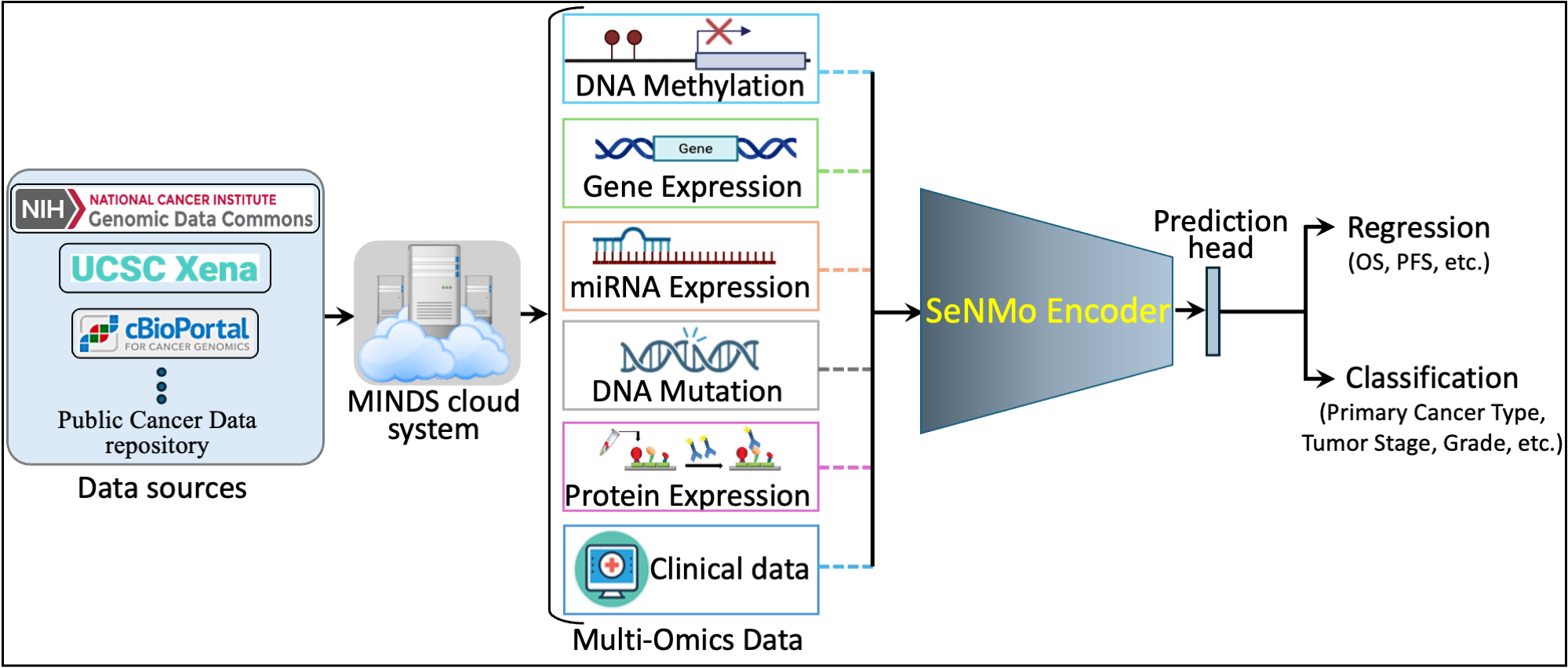
Figure 1: Overview of the SeNMo framework. Data from public and private sources are collected and curated through the MINDS system [28]. The resulting cohorts of multimodal data is preprocessed and fed to the self-normalizing deep learning encoder network that learns the cross-modality, pan-cancer features. The learned encoder weights can be used for different downstream tasks such as predicting overall survival (OS), progression-free survival (PFS), or cancer classification using different prediction heads.

2 Materials and Methods

2.1 Datasets

2.1.1 Data Acquisition

The Cancer Genome Atlas (TCGA) houses one of the largest collections of high-dimensional multi-omics data sets for more than 33 different types of cancer for around 20,500 individual tumor samples [48]. The multi-omics data contains high-throughput RNA-Seq, DNA-Seq, miRNA-Seq, single-nucleotide variant (SNV ), copy number variation (CNV ), DNA methylation, and reverse phase protein array (RPPA) data [48]. Building cohorts for patient data lying across different data formats, modalities, and systems is not a trivial task. To curate the data and build the patient cohorts, we used our previously developed Multimodal Integration of Oncology Data System (MINDS) which is a metadata framework for fusing data from publicly available sources such as the TCGA’s Genomic Data Commons (GDC) and UCSC Xena portal [55] into a machine-learning ready format [28]. MINDS is available as open-source for the cancer research community and we have integrated MINDS into the SeNMo framework for enhanced outreach and benefit of researchers. We used pan-cancer data comprising 33 cancer types from TCGA and Xena for training, validation, and testing of our model. We used the CPTAC-LSCC data and Moffitt Cancer Center’s internal Lung SCC data for evaluating the model’s performance off-the-shelf. We also fine-tuned the model on the CPTAC-LSCC [56] and Moffitts’ LSCC [57] data to evaluate the model’s generalizability and transfer learning capabilities.

2.1.2 Data Modalities

Out of the 13 multi-omic modalities contained across each GDC-TCGA cancer database, the ones chosen were gene expression RNAseq, DNA methylation, miRNA stem-loop expression, reverse phase protein array (RPPA) data, DNA mutation, and clinical data. The rationale behind selecting these specific modalities was that these modalities have been frequently preferred over the other data types in studying cancer primarily due to their direct relevance in the fundamental processes of cancer progression, their diagnostic and prognostic capabilities, and their established technologies [58, 17]. These modalities directly influence and reflect key biological processes fundamental to cancer progression, making them extremely valuable for uncovering the molecular mechanisms driving the disease [58]. Moreover, the set of these modalities provides robust predictive and prognostic information, and their integration provides a holistic view of a tumor’s multi-omic profile [59, 58, 17]. Lastly, the selected modalities contained a static feature number across each cancer type that helped us in developing the standard data pre-processing pipeline for pan-cancer studies. Below we briefly describe each of the data modalities considered in this study, followed by the preprocessing steps undertaken to select the features used in training the SeNMo model.

1. DNA Methylation: DNA methylation is a key epigenetic modification where methyl groups are added to the DNA molecule, typically at cytosine bases adjacent to guanine, known as CpG sites [60]. This process plays a crucial role in regulating gene expression without altering the DNA sequence itself [60]. In the context of cancer, DNA methylation patterns are immensely valuable as a data modality. Aberrant methylation of certain genes can lead to their silencing or activation, contributing to oncogenesis and tumor progression [61]. By analyzing methylation profiles across different cancer types, researchers can identify diagnostic markers, predict disease progression, and tailor personalized treatment strategies [61]. Thus, DNA methylation serves as a critical biomarker in oncology, offering insights into the molecular mechanisms of cancer and enhancing the precision of therapeutic interventions [61]. DNA methylation is quantified through beta values, which range from 0 to 1, with higher values indicating increased methylation [62]. The beta values for DNA methylation data in TCGA-GDC were measured using the Illumina Human Methylation 450 platform, a sophisticated method for detailed methylation profiling [63]. The data consists of 485,576 unique cg and rs methylation sites across several tumor types [63].

2. Gene Expression RNAseq: Gene expression analysis via RNA sequencing (RNAseq) is a powerful data modality in cancer research, providing deep insights into the transcriptomic landscape of tumors [64]. This technique quantifies the presence and quantity of RNA in a biological sample at a given moment, allowing for a detailed view of transcriptional activity in a cell [64]. RNAseq helps to identify genes that are upregulated or downregulated in cancer cells compared to normal cells, offering clues about oncogenic pathways and potential therapeutic targets [65]. The data derived from RNAseq are crucial for understanding the molecular mechanisms driving cancer progression and for developing targeted treatments that can selectively affect cancerous cells without impacting normal tissue [65]. This modality not only supports the identification of biomarkers for diagnosis and prognosis but also aids in the personalization of cancer therapy, making it a cornerstone of precision oncology [65]. The TCGA-GDC gene expression data is derived from RNA sequencing (RNAseq), utilizing High-throughput sequence Fragments Per Kilobase of transcript per Million mapped reads (HTseq-FPKM) as a measure for normalization [66]. This approach normalizes raw reads counts by gene length and the number of mapped reads. Further processing includes incrementing the FPKM value by one and then applying a log transformation to stabilize variance and enhance statistical analysis [67]. The data spans 60,483 genes, with FPKM values indicating gene expression levels—values over 1000 signify high expression, whereas values between 0.5 and 10 indicate low expression [66, 68].

3. miRNA Stem Loop Expression: miRNA stem loop expression is a pivotal aspect in understanding the intricate regulatory mechanisms that miRNAs, or microRNAs, play in gene expression [69]. These small, non-coding RNA molecules typically function by binding to complementary sequences on target messenger RNA (mRNA) transcripts, leading to their silencing [69]. The expression of miRNAs involves a multi-step process, that ensures specific targeting and effective modulation of gene expression, crucial for both normal cellular function and pathological conditions, such as cancer, where miRNA expression profiles can markedly differ from those in healthy tissue [69]. The miRNA expression values for TCGA-GDC were measured using stem loop expression through illumina and values were transformed by adding one and being log transformed [70, 71]. These were mapped across 1880 features representing typical hsa-miRNA sites, where, like gene expression, expressions varied between high and low values.

4. Protein Expression: Reverse Phase Protein Array is an effective methodology that is similar to western blotting, and is used to quantify protein expression in tissue slides [72]. The technique involves transferring antibodies to a nitrocellulose-coated slide to bind specific proteins, forming quantifiable spots through a DAB calorimetric reaction and tyramide dye deposition, analyzed using "SuperCurve Fitting" software [72, 73]. This process allows for effective comparison of protein expression levels in tumor samples against benign samples, highlighting aberrant protein levels that drive the molecular phenotypes of cancer [72, 74]. Similarly, through the quantification of protein expression, RPPA uncovers the functional status of several signaling molecules, phosphorylation molecules, and metabolic molecules [73]. RPPA data has been generated from the profiling of nearly 500 antibody-proteins for a given patient and deposited in The Cancer Proteome Atlas (TCPA) portal [75]. Each data file contains 488 antigen ID (AGID), the peptide target ID, gene identifier that codes for the protein, various other identifiers, and the antigen’s corresponding expression level. Protein expression levels were normalized through log transformation and median centering after being calculated by the SuperCurve fitting software [76].

5. DNA Mutation:

   When a particular DNA is sequenced, oftentimes the first step is to determine which regions are mutated compared to a reference genome (also known as DNA-seq analysis) [77]. These differences in alignments are subsequently captured in a variant calling format (VCF) file, which encapsulates the characteristics (chromosome, position, base mutated, other features, etc.) of the differing regions [78]. When VCF files are further aggregated to remove low quality variants and only include somatic mutations, they produce Mutation Annotation Format (MAF) format files [79]. MAF files also only consider the most affected reference for comparison, while VCF files consider all reference transcripts [77]. Like VCF files, MAF files include characteristics of the mutations such as the start position, end position, reference allele, type of mutation (deletion, insertion, polymorphism), but also include many different quantifiable scores that assess the translational impact of the mutation with references to other databases that provide the clinical significance [79]. Such information is of high relevance since mutations of clinical significance usually contain large defects in protein structure, and this greatly affects the protein’s downstream function. This dysregulation ultimately makes such mutations the driving force behind the development of several cancers [80]. SIFT and PolyPhen are features within MAF files that quantify a mutation’s effect on its encoded protein and can be further analyzed. MAF files from TCGA-GDC each have a varying number of rows, as different samples have a different number of mutations, but each row contains 126 mutational characteristics [79]. Analyzing MAF files not only aids in the identification of biomarkers for diagnosis and prognosis but also supports the personalization of targeted cancer therapy, thereby establishing it as a cornerstone of precision oncology [58, 81].

6. Clinical Data: Clinical data plays a crucial role in cancer research, serving as the foundation for correlating biological data with patient outcomes and demographics [4]. The clinical data encompasses detailed patient information, which is instrumental in understanding the epidemiology of cancer, evaluating treatment responses, and improving prognostic assessments [4]. Integrating clinical data with genomic and proteomic analyses can uncover relationships between molecular profiles and clinical manifestations of cancer [9]. Among the many clinical features and phenotypes available, age, gender, race, and cancer stage are particularly emphasized in cancer research due to their significant impact on disease presentation, progression, and treatment efficacy [82, 83, 84, 85]. Age is a critical factor as the incidence and type of cancer often vary significantly with age, influencing both the biological behavior of tumors and the overall prognosis of patients [82]. Gender is another key determinant, as certain cancers are gender-specific, while others may show differences in occurrence and outcome between men and women, likely due to biological, hormonal, and social factors [83]. Race has been linked to differences in cancer susceptibility, mortality rates, and treatment outcomes, reflecting underlying genetic, environmental, and socioeconomic factors [84]. Finally, cancer stage at diagnosis is paramount for determining the extent of disease and guiding treatment decisions, directly correlating with survival rates [85]. These four features are prioritized because they can be consistently measured, provide fundamental insights into the patient’s condition, and are predictive of clinical outcomes, making them indispensable in both research and clinical settings.

2.1.3 Pre-processing

Multiomics data integrates diverse biological data modalities such as genomics, transcriptomics, proteomics, and metabolomics, to understand the complex mechanisms of diseases like cancer. However, before integration, this data requires multiple preprocessing steps to overcome the big p, small n problem and other associated challenges of high-throughput molecular data. Some of the most significant challenges include, (i) data heterogeneity, where each type of data encompasses unique properties and scales, (ii) volume and complexity, where overwhelming volume of data (often in terabytes), managing, storing, and processing requires substantial computational resources and advanced data management strategies, (iii) quality and variability incurred because of the different platforms resulting in batch effects, differing levels of sensitivity, noise, missingness, and varying error rates, and (iv) lack of standardization in how data is collected and processed across different laboratories and studies. These challenges are further pronounced when selecting the preprocessing steps to make the data machine learning-ready. Some of the tasks to consider while dealing with multi-omic data include:

1. Normalization and Scaling. Because of the diverse nature, each type of omics data requires specific normalization techniques to adjust for factors. (i.e. gene length in RNA-seq data or protein abundance in proteomics). Choosing the right normalization method based on the type of data is crucial to ensure that data is comparable [86, 87, 88].

2. Handling Missing Data. Multiomics datasets often contain missing values due to detection limits or experimental errors. At times, as in our case, an entire data modality for a patient is missing. Selecting the robust imputation method for missing data is critical to avoid biased interpretations. Typical imputation methods suggest using mean, median, KNN, Gaussian mixture clustering, Bayesian, and deep learning-based (autoencoders) techniques to handle imputations [89].

3. Dimensionality Reduction. The high dimensionality of multiomics data often exceeds the number of samples available, leading to the risk of overfitting. Techniques like principal component analysis (PCA), t-distributed stochastic neighbor embedding (t-SNE), features selection, features engineering and others are used to reduce dimensionality while preserving the most informative features of the data [90].

4. Data Annotation and Metadata. Proper annotation and comprehensive metadata are essential for the effective preprocessing of multiomics data. Metadata must capture details about sample collection, processing protocols, and experimental conditions, which are crucial for accurate data interpretation and reproducibility [91].

5. Integration Techniques. Integrating diverse datasets involves sophisticated statistical and computational methods. Techniques such as concatenation, transformation, and advanced modeling (ML/ DL algorithms) are usually used to merge these datasets coherently [92].

Addressing these challenges requires interdisciplinary expertise, including bioinformatics, statistics, and domain-specific knowledge. The pan-cancer multiomics data comes with intra- and inter-dataset correlations, heterogeneous measurement scales, missing values, technical variability, and other background noise. Here we describe the preprocessing steps that were used across molecular data modalities.

• Remove NaNs. First, we removed the features that had NaNs across all the samples. This reduced the dimension, removed noise, and ensured continuous-numbered features to work with.

• Drop constant features. Next, constant/quasi constant features with a threshold of 0.998 were filtered out using Feature-engine, a A Python library for feature engineering and selection [93]. This eliminated features with no expression at all across every sample along with features that were noise, since the expression value was the same across every sample.

• Remove duplicates features. Next, duplicate features between genes were identified that contained the same values across two seperate genes, and one of the genes were kept. This may reveal gene-gene relationships between the two genes stemming from a up-regulation pathway or could simply reflect noise.

• Remove colinear features. Next, we filtered the features having low variance ($\approx$0.25) because we the features having high variance hold the maximum amount of information [94]. We used VarianceThreshold feature selector of scikit learn library that removes low-variance features based on the defined threshold [95]. We chose a threshold for each data modality so that the resulting features have the matching dimensions, as shown in Figure 2.

• Remove low-expression genes. The gene expression data originally contained 60,483 features, with FPKM transformed numbers ranging from 0 to 12. Roughly 30,000 genes remained after the above-mentioned preprocessing steps, which was still a very high number of features. High expression values reveal important biological insights due to an indication that a certain gene product is transcribed in large quantities, revealing that gene features with large expression values within the dataset are highly relevant. Genes containing an expression value greater than 7 (127 FPKM value) were kept, while the rest were discarded. Around 3000 genes remained after this process, all of which ranged from values between 7 and 12.

• Handle missing features. We handled missing features at two levels of data integration separately. For the features within each modality and within each cancer type, the missing values were imputed with the mean of the samples for that feature. This resulted in the full-length features vector for each sample. Across different cancers and across different modalities, we padded the missing features with zeros. One may opine that this is equivalent to zero-padding prevalent in the bio-statistics, but we argue that padding zeros across cancers and modalities is not imputation when integrating very high dimensional, and high-sample sized data. Moreover, zero-padding has also been shown to improve the quality of gene studies results across disease data including breast cancer [96]. In deep learning, zero imputation technique shows the best performance compared to other imputation techniques and deficient data removal techniques [97, 98]. Moreover, there is a line of work that simply used zero padding by to minimize the noise in data and achieved state-of-the-art performance on respective datasets [99, 100, 101]

2.1.4 Features integration

After carrying out the preprocessing steps mentioned above, we integrate the data across cancers and across modalities. We generate two views of the data by concatenating the features across cancers and across modalities. First view is created by taking the union of features across all cancer patients for each of the six modalities (DNA methylation, gene expression, miRNA expression, protein expression, DNA mutation, and clinical). The DNA methylation data originally had 485,576 features across all cancers, which was reduced to $\approx$ 4500 features. Union of these features resulted in the feature dimension of 52,396. The gene expression data originally had 60,483 features across all cancers, which was reduced to $\approx$ 300 features. Union of these features resulted in the feature dimension of 8794. The miRNA expression data originally had 1880 features across all cancers, which was reduced to $\approx$ 1400 features. Union of these features resulted in the feature dimension of 1730. The protein expression data originally had 487 features across all cancers, which was reduced to 472 features unionized to 472 dimensions. The DNA mutation data had 18,090 features across all cancers, pre-processed and unionized to 17,253 features. Lastly, we convert the categorical clinical features to numerical values such as gender, race, and cancer stages. The details of these clinical characteristics are given in Table 2. Mathematically, the preprocessing is given below.

Let $D$ represent the initial feature having fixed dimension for each cancer. The dimension of each feature set is reduced through a preprocessing step to $\tilde{D}$, which is calculated by a function of $D$, noted as $f(D)$, where $f$ is the dimension reduction function such as those presented in the previous section, $\tilde{D}=f(D)$. The reduced dimensions $\tilde{D}$ from each cancer type are then combined through a union operation to generate a feature vector $D_{m}$ for each modality $m$ and $M=6$ are the total number of modalities. For $n=33$ cancer types and $\tilde{D}$ is the preprocessed, reduced dimension feature vector, the $D_{m}$ is the union of these dimensions. Finally, the union of all $D_{m}$ across different modalities results in the total pan-cancer, multimodal feature vector dimension $D_{c}\in\mathbb{R}^{80,697}$. The feature vector dimension for each modality, $D_{m}$, is defined as:

$$D_{m}=\begin{cases}\bigcup_{i=1}^{n}\tilde{D}_{i}&\text{if }\tilde{D}_{i}\text{ varies by cancer type or modality,}\\ \tilde{D}&\text{otherwise.}\end{cases}$$ (1)

The total pan-cancer, multimodal feature vector dimension $D_{c}$ can then be expressed as:

$$D_{c}=\bigcup_{m=1}^{M}D_{m}$$ (2)

Table 1: Feature Reduction Summary of Pan-cancer data.

Data	Primary Site	Cases	miRNA Exprn		DNA Methyl		Gene Exprn		Protein Exprn		DNA Mut
			Before	After	Before	After	Before	After	Before	After	Before	After
TCGA-DLBC	Large B-cell Lymphoma	51	1880	1060	485576	4396	60483	850	487	472	18090	17253
TCGA-UCS	Uterine Carcinosarcoma	61	1880	1101	485576	4632	60483	1231	487	472	18090	17253
TCGA-CHOL	Bile Duct	62	1880	967	485576	4479	60483	1261	487	472	18090	17253
TCGA-UVM	Uveal melanomas	80	1880	1162	485576	4019	60483	772	487	472	18090	17253
TCGA-MESO	Mesothelioma	86	1880	1158	485576	4372	60483	1278	487	472	18090	17253
TCGA-ACC	Adrenocortical	95	1880	1110	485576	4454	60483	1304	487	472	18090	17253
TCGA-THYM	Thymoma	138	1880	1245	485576	4609	60483	1337	487	472	18090	17253
TCGA-TGCT	Testicular	139	1880	1290	485576	4762	60483	1343	487	472	18090	17253
TCGA-READ	Rectal	178	1880	1314	485576	4077	60483	1547	487	472	18090	17253
TCGA-KICH	Kidney Chromophobe	182	1880	1089	485576	4333	60483	1107	487	472	18090	17253
TCGA-PCPG	Pheochromocytoma and Paraganglioma	189	1880	1251	485576	4550	60483	1216	487	472	18090	17253
TCGA-PAAD	Pancreatic	222	1880	1308	485576	4518	60483	1567	487	472	18090	17253
TCGA-ESCA	Esophageal	249	1880	1300	485576	4192	60483	1684	487	472	18090	17253
TCGA-SARC	Sarcoma	287	1880	1235	485576	4467	60483	2490	487	472	18090	17253
TCGA-CESC	Cervical	304	1880	1405	485576	4167	60483	2017	487	472	18090	17253
TCGA-KIRP	Kidney Papillary Cell Carcinoma	376	1880	1297	485576	4078	60483	1798	487	472	18090	17253
TCGA-SKCM	Skin Cutaneous Melanoma	436	1880	1426	485576	4427	60483	2488	487	472	18090	17253
TCGA-BLCA	Bladder	447	1880	1361	485576	4483	60483	2751	487	472	18090	17253
TCGA-LIHC	Liver	463	1880	1336	485576	4023	60483	2017	487	472	18090	17253
TCGA-STAD	Stomach	499	1880	1397	485576	4196	60483	2354	487	472	18090	17253
TCGA-LGG	Lower Grade Glioma	533	1880	1287	485576	4193	60483	1560	487	472	18090	17253
TCGA-COAD	Colon	539	1880	1460	485576	4671	60483	1931	487	472	18090	17253
TCGA-UCEC	Endometrioid	588	1880	1414	485576	4424	60483	2849	487	472	18090	17253
TCGA-HNSC	Head and Neck	611	1880	1428	485576	4358	60483	2059	487	472	18090	17253
TCGA-THCA	Thyroid	614	1880	1369	485576	4160	60483	1432	487	472	18090	17253
TCGA-PRAD	Prostate	623	1880	1334	485576	4006	60483	1635	487	472	18090	17253
TCGA-LAML	Acute Myeloid Leukemia	626	1880	1140	485576	4415	60483	1032	487	472	18090	17253
TCGA-GBM	Glioblastoma	649	1880	1023	485576	4076	60483	1206	487	472	18090	17253
TCGA-LUAD	Lung Adenocarcinoma	728	1880	1360	485576	4480	60483	2562	487	472	18090	17253
TCGA-OV	Ovarian	731	1880	1430	485576	4254	60483	2116	487	472	18090	17253
TCGA-LUSC	Lung Squamous Cell Carcinoma	752	1880	1375	485576	4302	60483	2610	487	472	18090	17253
TCGA-KIRC	Kidney Clear Cell Carcinoma	979	1880	1333	485576	4399	60483	2274	487	472	18090	17253
TCGA-BRCA	Breast	1260	1880	1418	485576	4195	60483	3671	487	472	18090	17253

Table 2: Summary of patient characteristics for pan-cancer data used in this study.

Cancer Type	No. of Cases	Age (Mean±SD)	Gender (M/F)	Race (White/Asian/Black/NA/American Indian/Alaska/Islander)	Stage (0/I/IA/IB/IC/II/IIA/IIB/IIC/III/IIIA/IIIB/IIIC/IV/IVA/IVB/IVC/NA)
TCGA-ACC	95	47.46 ± 16.2	33/62	79/3/1/12/0/0	0/9/0/0/0/46/0/0/0/20/0/0/0/17/0/0/0/3
TCGA-BLCA	447	67.92 ± 10.39	326/121	363/43/23/18/0/0	0/3/0/0/0/136/0/0/0/159/0/0/0/148/0/0/0/1
TCGA-BRCA	1260	57.94 ± 13.11	13/1247	915/59/198/87/1/0	0/114/94/7/0/6/404/307/0/2/176/30/74/22/0/0/0/24
TCGA-CESC	304	48.04 ± 13.7	0/304	211/19/32/30/9/0	0/0/0/0/0/0/0/0/0/0/0/0/0/0/0/0/0/304
TCGA-CHOL	62	64.37 ± 12.21	30/32	55/3/3/1/0/0	0/30/0/0/0/16/0/0/0/5/0/0/0/2/3/6/0/0
TCGA-COAD	539	66.93 ± 12.67	288/251	261/11/67/198/2/0	0/87/1/0/0/46/150/13/2/26/9/69/47/56/18/3/0/12
TCGA-DLBC	51	56.76 ± 13.68	24/27	32/18/1/0/0/0	0/0/0/0/0/0/0/0/0/0/0/0/0/0/0/0/0/51
TCGA-ESCA	249	64.22 ± 12.11	208/41	162/46/6/35/0/0	0/14/9/7/0/1/56/43/0/41/16/10/9/7/6/0/0/30
TCGA-GBM	649	57.74 ± 14.32	399/250	547/13/53/36/0/0	0/0/0/0/0/0/0/0/0/0/0/0/0/0/0/0/0/649
TCGA-HNSC	611	61.02 ± 11.92	443/168	522/12/58/17/2/0	0/29/0/0/0/93/0/0/0/97/0/0/0/0/302/13/1/76
TCGA-KICH	182	51.61 ± 14.12	99/83	154/6/19/3/0/0	0/75/0/0/0/59/0/0/0/34/0/0/0/14/0/0/0/0
TCGA-KIRC	979	60.67 ± 11.95	641/338	876/16/73/14/0/0	0/475/0/0/0/102/0/0/0/237/0/0/0/161/0/0/0/4
TCGA-KIRP	376	61.98 ± 12.2	278/98	275/6/75/16/4/0	0/219/0/0/0/25/0/0/0/77/0/0/0/21/0/0/0/34
TCGA-LAML	626	54.82 ± 15.87	345/281	564/8/49/5/0/0	0/0/0/0/0/0/0/0/0/0/0/0/0/0/0/0/626
TCGA-LGG	533	42.71 ± 13.32	293/240	492/8/22/10/1/0	0/0/0/0/0/0/0/0/0/0/0/0/0/0/0/0/533
TCGA-LIHC	463	60.44 ± 13.71	305/158	255/168/25/14/1/0	0/211/0/0/0/105/0/0/0/6/78/12/11/2/1/3/0/34
TCGA-LUAD	728	65.20 ± 10.08	329/399	580/14/84/48/2/0	0/7/194/195/0/2/67/103/0/0/101/12/0/37/0/0/0/10
TCGA-LUSC	752	67.28 ± 8.62	548/204	530/12/47/163/0/0	0/4/127/243/0/4/87/138/0/3/94/33/0/12/0/0/0/7
TCGA-MESO	86	63.01 ± 9.78	70/16	84/1/1/0/0/0	0/7/2/1/0/15/0/0/0/45/0/0/0/16/0/0/0/0
TCGA-OV	731	59.60 ± 11.44	0/731	626/25/43/33/3/0	0/0/0/0/0/0/0/0/0/0/0/0/0/0/0/0/731
TCGA-PAAD	222	64.87 ± 11.36	123/99	195/13/8/6/0/0	0/1/6/15/0/0/36/148/0/6/0/0/0/7/0/0/0/3
TCGA-PCPG	189	47.02 ± 15.15	84/105	157/7/20/4/1/0	0/0/0/0/0/0/0/0/0/0/0/0/0/0/0/0/189
TCGA-PRAD	623	60.93 ± 6.8	623/0	510/13/81/18/1/0	0/0/0/0/0/0/0/0/0/0/0/0/0/0/0/0/623
TCGA-READ	178	63.83 ± 11.85	98/80	90/1/7/80/0/0	0/37/0/0/0/7/40/2/1/6/7/25/14/21/7/0/0/11
TCGA-SARC	287	60.70 ± 14.38	129/158	253/5/20/9/0/0	0/0/0/0/0/0/0/0/0/0/0/0/0/0/0/0/287
TCGA-SKCM	436	57.84 ± 15.41	289/174	441/12/1/9/0/0	6/30/18/30/0/39/18/28/61/44/16/46/68/23/0/0/0/36
TCGA-STAD	499	65.44 ± 10.53	320/179	311/108/15/64/0/0	0/1/21/46/0/37/54/71/0/4/88/67/39/47/0/0/0/24
TCGA-TGCT	139	31.87 ± 9.19	139/0	124/4/6/5/0/0	0/69/26/11/0/4/6/1/1/2/1/6/5/0/0/0/0/7
TCGA-THCA	614	47.17 ± 15.83	166/448	413/59/35/106/1/0	0/350/0/0/0/64/0/0/0/134/0/0/0/4/52/0/8/2
TCGA-THYM	138	58.12 ± 13	72/66	115/13/8/2/0/0	0/0/0/0/0/0/0/0/0/0/0/0/0/0/0/0/138
TCGA-UCEC	588	63.74 ± 11.06	0/588	402/21/120/32/4/0	0/0/0/0/0/0/0/0/0/0/0/0/0/0/0/0/588
TCGA-UCS	61	70.07 ± 9.24	0/61	50/1/9/1/0/0	0/0/0/0/0/0/0/0/0/0/0/0/0/0/0/0/61
TCGA-UVM	80	61.65 ± 13.95	45/35	55/0/0/25/0/0	0/0/0/0/0/0/12/27/0/0/25/10/1/4/0/0/0/1
Moffitt-LSCC	108	69.14 ± 8.34	72/36	105/0/3/0/0/0	0/0/24/25/0/0/31/15/0/0/12/1/0/0/0/0/0/0

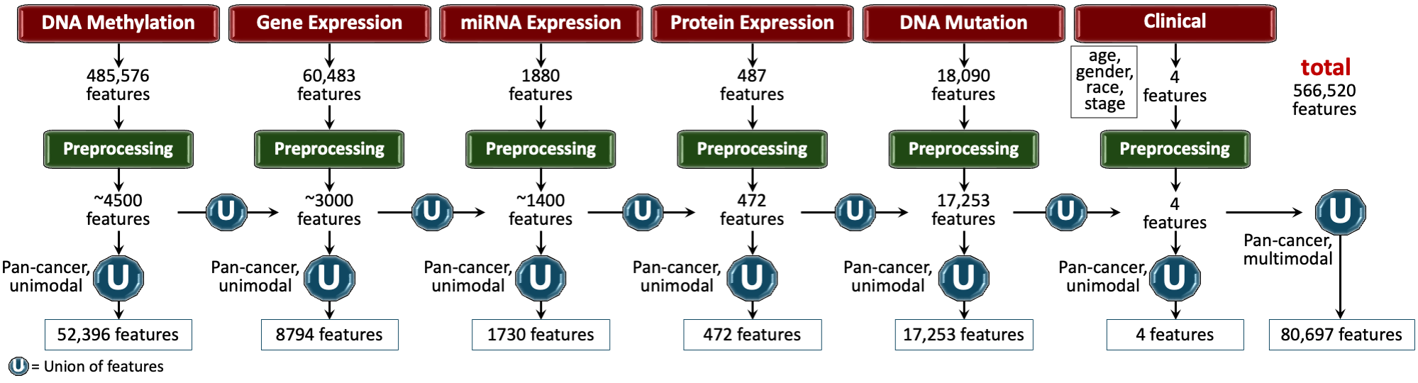
Figure 2: Features processing pipeline for pan-cancer data.

2.2 Clinical end-points

To assess the performance of the SeNMo framework, we chose two end-points that belong to two different categories of machine learning tasks. First is the clinically relevant prediction of overall survival (OS) which is a regression task. The second is the prediction of the primary cancer type which is 33-class classification task.

2.2.1 Overall Survival (OS)

Cancer prognosis via survival outcome prediction is a standard method used for biomarker discovery, stratification of patients into distinct treatment groups, and therapeutic response prediction [102]. Advancements in next-generation sequencing have led to a surge in data availability [28]. Statistical survival models and a shift towards incorporating deep learning into survival analysis has improved the task of OS prediction. Previous works have used combinations of molecular data types and employed different statistical and learning-based methods to predict OS in different datasets [103, 33, 35, 36]. The journey towards comprehensive survival analysis continues, aiming to combine different data types to better understand the relationship between molecular features and patient outcomes, ultimately leading to more precise prognostic assessments and tailored treatment approaches. In this study, we utilize clinical, demographic, genomic, and molecular data types to investigate potential risk factors for cancer patients, specifically examining their correlations with the patients’ time-to-event, which in this case is overall survival. We have implemented prediction of OS as a regression task, i.e., prediction of OS in days. Time-to-event or survival data not only records the occurrence of events like death but also tracks the time from the study’s outset to when the event happens, tracks when the study concludes, or tracks when a patient is no longer followed (known as right censoring). Survival or right-censored times since cancer diagnosis for our pan-cancer data is depicted in Figure 3A. Due to censoring, the exact survival time for some patients remains unknown. In such instances, each patient’s outcome is defined by two main variables: a censoring indicator, also called the status, and the observed time $T=\min(T_{s},T_{c})$, where ${T}_{s}$ represents the exact survival time and ${T}_{c}$ is the censoring time, $\{{T}_{s}\leq{T}_{c}\}$ [10]. Survival function to describe the likelihood of a patient surviving beyond a specified time $t$, is given as:

$$F(t)=P\{T>t\}$$ (3)

Additionally, the hazard function offers insights into the risk of the event occurring at a given time, assuming survival up to that point. Hazard function represents the instantaneous rate at which events (such as death) occur at a specific time, given that the individual has survived up to that time. It provides insights into the risk of experiencing the event at any given moment, conditional on having survived up to that point in time. Mathematically, the hazard function $h(t)$ is defined as the ratio of the probability of the event occurring in a small time interval around $t$ to the probability of surviving beyond $t$:

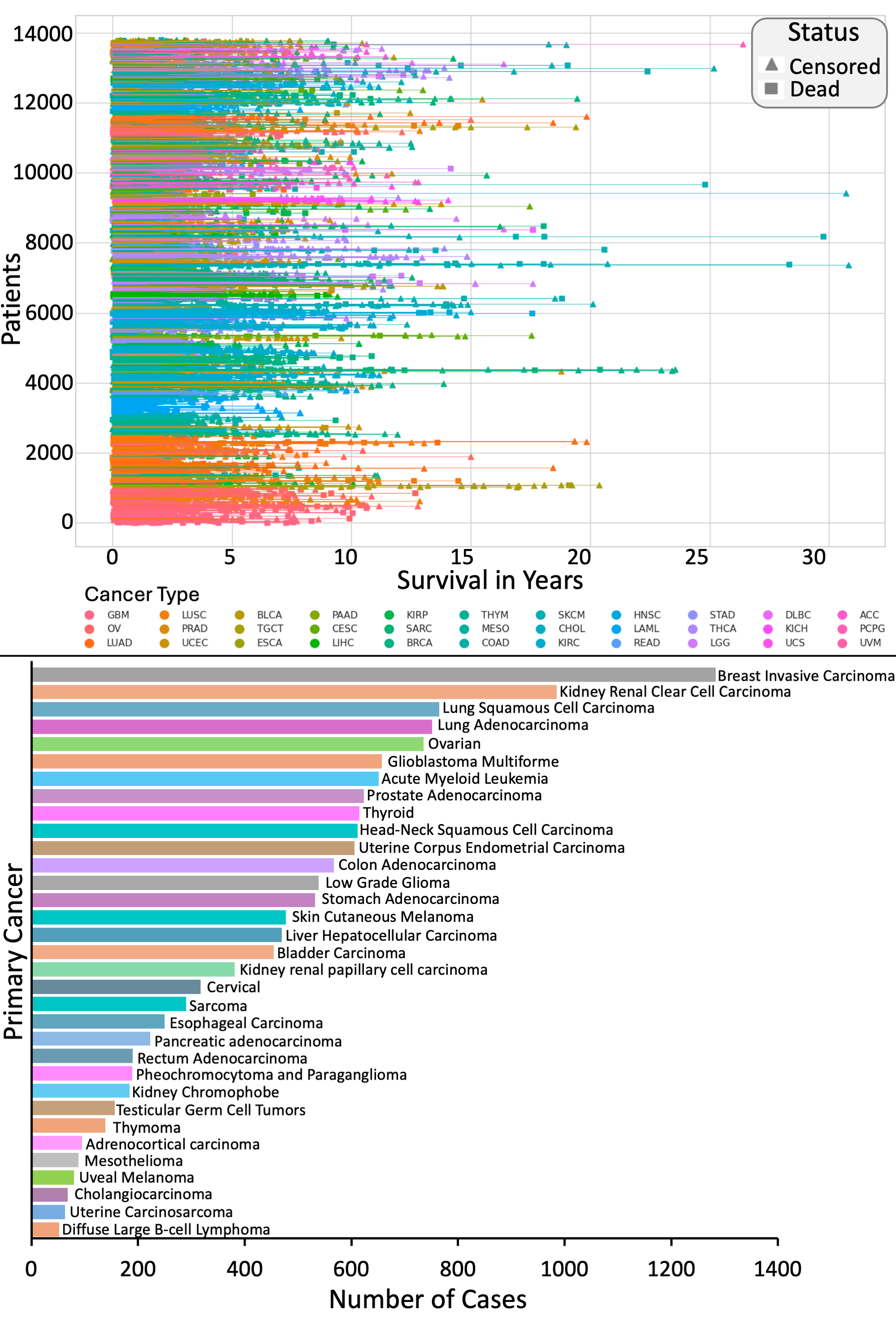
Figure 3: Summary of number of cases in the pan-cancer data.

$$h(t)=\lim_{\Delta t\to 0}\frac{P(t\leq T<t+\Delta t\,|\,T\geq t)}{\Delta t}$$ (4)

where:

• $h(t)$ is the hazard function at time $t$.

• $T$ is the survival time.

• $P(t\leq T<t+\Delta{t}\,|\,T\geq{t})$ is the conditional probability that the event occurs in the time interval $[t,t+\Delta{t})$ given that survival time is greater than or equal to $t$.

• $\Delta{t}$ represents an infinitesimally small time interval.

Hazard function describes the instantaneous risk of experiencing the event of interest at any given time, based on survival data. In our pan-cancer data, the (right)censoring was defined as $censor=1$ in case of an event (death), and $0$ otherwise.

2.2.2 Primary Cancer type

The primary cancer type prediction task involves classifying a cancer sample into one of 33 possible types based on various biological and clinical features. This task is fundamentally important and clinically relevant because accurate identification of the primary cancer type is critical for choosing the most effective treatment strategy, improving patient outcomes, and personalizing therapy approaches [104]. Cancer treatments and prognostics can vary dramatically between different cancer types, often requiring specific interventions that are tailored to the unique biological characteristics of each type. Correctly predicting the primary cancer type helps in planning follow-up care and surveillance, enhancing the likelihood of early detection of recurrence. Thus, achieving high accuracy in this classification not only supports better clinical decision-making but also significantly impacts patient survival and quality of life. The pan-cancer data comprising of 33 cancers and distribution of patients (cases) across these datasets are depicted in Figure 3B.

2.3 SeNMo Deep Learning Model

In learning scenarios with hundreds to thousands of features and relatively few training samples, Feedforward networks are susceptible to overfitting [102]. Unlike Convolutional Neural Networks (CNNs), the weights in Feedforward networks are shared, making them more prone to training instabilities caused by perturbations and regularization techniques like stochastic gradient descent and Dropout. CNNs do not perform as well on high-dimensional, low-sample data for several reasons including the spatial invariance assumption, fixed input size, and parameter efficiency viz-a-viz multiomics data sparsity. Transformers-based models are also not inherently optimized for high-dimensional, low-sample data, such as in genomics or other multiomics datasets, due to the fact that these models use attention mechanism to predict the next token in case of language tasks and meaningful patterns in non-language tasks, which fails in case of highly sparse molecular data. To address overfitting in high-dimensional, low-sample-size multiomics data and employ more robust regularization techniques during training, we draw inspiration from Self-Normalizing Networks (SNN) introduced by Klambauer et al. [105]. SNNs have been extensively used for their ability to effectively handle high-dimensional data with limited samples, making them particularly relevant in the field of multiomics data analysis. Our learning framework is based on the stacked layers of SNNs, as described below.

As shown in Figure 4, SeNMo comprises of stacked blocks of SNN layers, where each block is composed of a linear unit, SELU activation, followed by Alpha dropout. Combined, these blocks enable high-level abstract representations by keeping neuron activations converged towards zero mean and unit variance [105]. Linear unit is essentially equivalent to what is commonly referred to as a “fully connected (FC) layer" or a “multilayer perceptron (MLP) layer" in traditional neural network architectures. SELU activations are an alternative to the traditional rectified linear unit (ReLU) activations commonly used in neural networks. Klambauer et al. demonstrated through the Banach fixed-point theorem that activations with close proximity to zero mean and unit variance, propagating through numerous network layers, will ultimately converge to zero mean and unit variance [105]. SELU activations have the unique property of self-normalization, meaning that the activations tend to converge to a mean of zero and a standard deviation of one, regardless of the input distribution. The mathematical equation for the SELU activation function is:

$$selu(x)=\lambda\begin{cases}x&\text{if }x>0\\ \alpha(e^{x}-1)&\text{if }x\leq 0\end{cases}$$ (5)

where:

• $\lambda$ is a scaling factor (typically set to $1.05071$).

• $\alpha$ is the negative scale factor (typically set to $1.6733$).

Dropout is a regularization technique that randomly sets a fraction of input units to zero during training to prevent overfitting. Alpha dropout is a modified version of traditional dropout regularization, specifically designed to preserve the self-normalizing property of SELU activations. Alpha Dropout applies a dropout mask to the activations during training, scaled by a factor that ensures the mean and variance of the activations remain unchanged. This scaling factor is computed based on the dropout rate and the SELU parameters ($\lambda$ and $\alpha$). Mathematically,

$$\text{AlphaDropout}(x)=\frac{x-\mu(x)}{std(x)}\times mask+\mu(x)$$ (6)

where:

• $x$ is the input activation.

• $\mu(x)$, $std(x)$ are mean and standard deviation of the input activation, respectively.

• $mask$ is a binary mask generated with the specified dropout rate.

Together, SELU activations and Alpha Dropout enable SeNMo blocks to maintain a stable mean and variance of activations throughout the network layers, facilitating more stable training and better generalization performance. Similarly, SELU activation and alpha dropout help mitigate training instabilities caused by vanishing or exploding gradients in the Feedforward networks. Our network architecture consists of seven fully-connected hidden layers followed by Exponential Linear Unit (ELU) activation and alpha dropout, where the number of neurons in each block is shown in the inset of Figure 4. The final fully-connected layer is utilized to learn a latent representation of the sample, which we call the patient embedding $x\in\mathbbm{R}^{48}$.

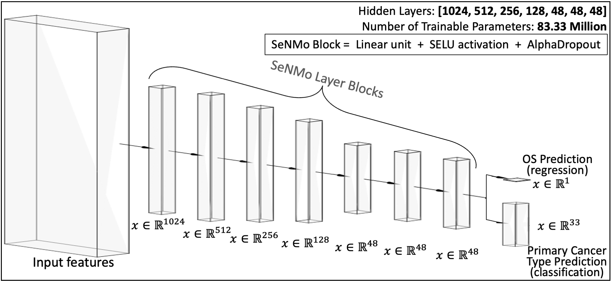
Figure 4: Architecture of the SeNMo encoder network. There are seven hidden layers each comprising of a linear unit, SELU activation, and Alpha dropout. The trained model has 83.33 million parameters. The number of neurons in each hidden layer, input layer and output layer are also depicted in the figure. The same model is used for regression and classification tasks.

2.4 Training and Evaluation

2.4.1 Evaluation

We evaluate SeNMo’s performance with the quantitative and statistical metrics common for survival outcome prediction and grade classification. For survival analysis, we evaluate the model using the Concordance Index (C-Index). For the primary cancer type classification, we generate the classification report comprising of average accuracy, average precision, recall, F1-score, confusion matrix, and scatter plot. For testing the statistical significance of the predictions, we use the Log Rank Test. Below we explain the evaluation metrics and statistical test in detail.

1. Loss Function: The loss being used for backpropagation in the model is a combination of three components: cox loss, cross-entropy loss, and regularization loss. This combined loss function aims to simultaneously optimize the model’s ability to predict survival outcomes (Cox loss), encourage model simplicity or sparsity (regularization loss), and model the likelihood of cancer types (cross-entropy loss). The overall loss is a weighted sum of these three components, where each component is multiplied by a corresponding regularization hyperparameter ($\lambda_{c}$, $\lambda_{ce}$, $\lambda_{r}$). This weighted sum allows for balancing the influence of each loss component on the optimization process. Mathematically, the overall loss can be expressed as:

   $$\text{L}=\text{$\lambda_{c}$}\text{$L_{cox}$}+\text{$\lambda_{ce}$}\text{$L_{ce}$}+\text{$\lambda_{r}$}\text{$L_{reg}$}$$ (7)

   • Cox proportional hazards loss ($L_{cox}$): The Cox loss is a measure of dissimilarity between the predicted hazard scores and the true event times in survival analysis. It is calculated using the Cox proportional hazards model and penalizes deviations between predicted and observed survival outcomes of all individuals who are at risk at time $t_{i}$, weighted by the censoring indicator [106]. The function takes a vector of survival times for each individual in the batch, censoring status for each individual (1 if the event occurred, 0 if censored), and the predicted log hazard ratio for each individual from the neural network, and returns the Cox loss for the batch, which is used to train the neural network via backpropagation. This backpropagation encourages the model to assign higher hazards to high-risk individuals and lower predicted hazards to censored individuals or who experience the event later. Mathematically, the Cox loss is expressed as:

     $$\text{$L_{cox}$}=-\frac{1}{N}\sum_{i=1}^{N}\left(\theta_{i}-\log\sum_{j=1}^{N}e^{\theta_{j}}\cdot R_{ij}\right)\cdot\text{censor}_{i}$$ (8)

     where:

     • $N$ is the batch size (number of samples).

     • $\theta_{i}$ is the predicted hazard for sample $i$.

     • $R_{ij}$ is the indicator function that equals 1 if the survival time of sample $j$ is greater than or equal to the survival time of sample $i$, and 0 otherwise.

     • $censor_{i}$ is the censoring indicator for sample $i$, which equals 1 if the event is observed for sample $i$ and 0 otherwise.

   • Cross-entropy loss ($L_{ce}$): The cross-entropy loss is a common loss function used for multi-class classification problems, particularly when each sample belongs to one of $C$ classes. When combined with a LogSoftmax layer, the function measures how well a model’s predicted log probabilities match the true distribution across various classes. For a multi-class classification problem having $C$ classes, the model’s outputs (raw class scores or logits) are transformed into log probabilities using a LogSoftmax layer. The cross-entropy loss compares these log probabilities to the true distribution, which is usually represented in a one-hot encoded format. The loss is calculated by negating the log probability of the true class across all samples in a batch and then averaging these values. For the given output of LogSoftmax, $\log(p_{n,c})$ for each class $c$ in each sample $n$, the cross-entropy loss for a multi-class problem can be defined as:

     $$\text{$L_{ce}$}=-\frac{1}{N}\sum_{n=1}^{N}\sum_{c=1}^{C}y_{n,c}\log(p_{n,c})$$ (9)

     where:

     • $N$ is the total number of samples.

     • $C$ are the total classes.

     • $y_{n,c}$ is the target label for sample $n$ and class $c$, typically 1 for the true class and 0 otherwise.

   • Regularization loss ($L_{reg}$): The regularization loss encourages the model’s weights to remain small or sparse, thus preventing overfitting and improving generalization.We used $L1$ regularization to the SeNMo’s parameters, which penalizes the absolute values of the weights.

2. Concordance Index (C-Index): The C-Index is a frequently used evaluation metric in survival analysis to assess the predictive accuracy of a model for the time-to-event outcomes [10]. It measures the degree to which the model’s predictions correlate with the actual survival times observed in the data. It quantifies the model’s ability to correctly rank pairs of subjects based on their predicted survival times. The C-Index evaluates the probability that, in a randomly selected pair of individuals, the one who experienced the event (like death or failure) first also had a higher risk score predicted by the model. Risk score is the output of the survival model and represents the expected order of the events; the higher the score, the higher the risk of experiencing the event sooner [10]. We used the $concordance\_index$ Lifelines function to calculate the C-Index. This function takes the predicted hazard scores for each individual, the true event indicators (e.g., 1 if an event occurred, 0 if censored) for each individual, and the survival times (time to event or censoring) for each individual. The C-Index function computes the fraction of all pairs of subjects whose predicted event times are correctly ordered among all pairs where one subject experienced an event and the other did not. C-Index ranges between 0 and 1 where 0.5 is the expected result from random predictions, 1.0 is a perfect concordance and, 0.0 is perfect anti-concordance [10]. Mathematically,

   $$\begin{split}\text{C-Index}&=\frac{(\text{Number of concordant pairs}+0.5\times\text{tied pairs})}{\text{Total number of evaluable pairs}},\\ \text{C-Index}&=\Pr(\hat{S}_{i}<\hat{S}_{j}|T_{i}<T_{j},\delta_{i}=1)\end{split}$$ (10)

   where:

   • Concordant pairs are pairs of individuals where the predicted survival times are correctly ordered relative to the observed survival times.

   • Tied pairs are number of pairs where the predictions are equal or survival times are the same.

   • Total number of evaluable pairs are the total pairs considered, excluding pairs with censoring issues or other exclusions.

   • $\hat{S}_{i}$ and $\hat{S}_{j}$ represent the predicted risks or survival probabilities for individuals $i$ and $j$, respectively.

   • $T_{i}<T_{j}$ implies that individual $i$ experienced the event before individual $j$.

   • $\delta_{i}=1$ indicates that the event for individual $i$ was observed (not censored).

3. Cox log-rank function: The Cox Log-rank function calculates the p-value using the log-rank test based on predicted hazard scores, censor values, and the true overall survival times. The log-rank test is a statistical method to compare the survival distributions of two groups, where the null hypothesis is that there is no difference between the groups. It is commonly used in survival analysis to compare the observed number of events in each group to the number of events expected under the null hypothesis. For the hazard ratio $h_{i}(t)$ of group $i$ at time $t$ is given by,

   $$\begin{split}&H_{0}:h_{1}(t)=h_{2}(t)\\ &H_{A}:h_{1}(t)=ch_{2}(t),\;\;c\neq 1\end{split}$$ (11)

   The test statistic for the log-rank test is calculated as the sum of the differences between the observed and expected number of events squared, divided by the expected number of events, summed over all observed time points. The p-value obtained from the log-rank test indicates the significance of the difference in survival distributions between the two groups. The test statistic is chi-squared under the null hypothesis [107].

   $$\chi^{2}=\sum_{i=1}^{N}\frac{(O_{i}-E_{i})^{2}}{E_{i}}$$ (12)

   where:

   • $O_{i}$ is the observed number of events at time point $i$ in the sample.

   • $E_{i}$ is the expected number of events at time point $i$ under the null hypothesis.

   • $N$ is the total number of observed time points.

2.4.2 Hyperparameters Search

Hyperparameters are non-learnable parameters of a deep learning model and are crucial as they govern the learning process and model architecture. Hyperparameter tuning involves selecting the optimal combination of parameters that results in the best model performance. Common hyperparameters include learning rate and policy, batch size, number of epochs, weight decay, dropout type and probability, and architecture specifics such as the number of hidden layers and neurons in each layer. Methods for hyperparameter search range from grid search, where all possible combinations of parameters are evaluated; to random search, which randomly samples parameter combinations within predefined bounds. More sophisticated techniques like Bayesian optimization or using automated machine learning (AutoML) tools can dynamically adjust parameters based on previous results to find the best solutions more efficiently. We employed weights and biases [108] utility to carry out random and Bayesian methods of hyperparameters search. The list of hyperparameters we searched for training and fine-tuning is given in Table 3. For model training, we conducted around 400 simulations to find the current hyperparameters. For fine-tuning the SeNMo model on CPTAC-LUSC and Moffitt’s Lung SCC data, we ran around 1000 and 450 simulations, respectively. The plots for these simulations are given in the appendix figures 9, 10, and 11.

Hyperparams	Training (range)	Finetuning (range)
Learning Rate	[1e-6, 1e-1]	[1e-8, 1e-3]
Weight Decay	[1e-6, 1e-1]	[1e-4, 1e-2]
Dropout	[0.1, 0.65]	[0.05, 0.45]
Batch Size	[64, 128, 256, 512]	[8, 16, 32, 48]
Epochs	[50, 100]	[8, 10, 15, 20, 30]
Hidden Layers	[1, 2, 3, 4, 5, 6, 7, 8, 9]	-
Hidden Neurons	[2048, 1024, 512, 256, 128, 48, 32]	-
Optimizer	[adam, sgd, rmsprop, adamw]	[adam, adamw]
Learning Rate Policy	[linear, exp, step, plateau, cosine]	[linear, exp, plateau]
Frozen Layers	-	[7, 6, 5, 4, 3, 2]
Additional Layers	-	[1, 2, 3]

Table 3: Hyperparameters for training and finetuning.

2.4.3 Frameworks, Compute resources, and wall-clock times

We trained SeNMo model using the Moffitt Cancer Center’s HPC machine with 1 Tesla V100 32GB GPU running Ubuntu 22.04.4 and CUDA 12.2. The entire code was developed in Python and PyTorch frameworks. The software frameworks and corresponding packages used in our codebase are given in Table 4. Training time for our current 83.33 Million parameter SeNMo encoder is approximately 11 hours. We conducted the hyperparameters search of the pan-cancer model for approximately 20 days using multiple GPUs in parallel. Finetuning the trained model on a given data having around 150 patients approximately takes 15 minutes. It took us one week to find the fine-tuning hyperparameters for the CPTAC-LSCC data.

Table 4: Frameworks and packages used in our codebase.

	Package name	Version
Operating systems	Ubuntu	20.04.4
Programming languages	Python	3.10.13
Deep learning framework	Pytorch	2.2.0
	torchvision	0.17.0
	feature-engine	1.6.2
	imbalanced-learn	0.12.0
Miscellaneous	scipy	1.12.0
	scikit-learn	1.4.0
	numpy	1.26.3
	PyYaml	6.0.1
	jupyter	1.0.0
	pandas	2.2.0
	pickle5	0.0.11
	protobuf	4.25.2
	wandb	0.16.3

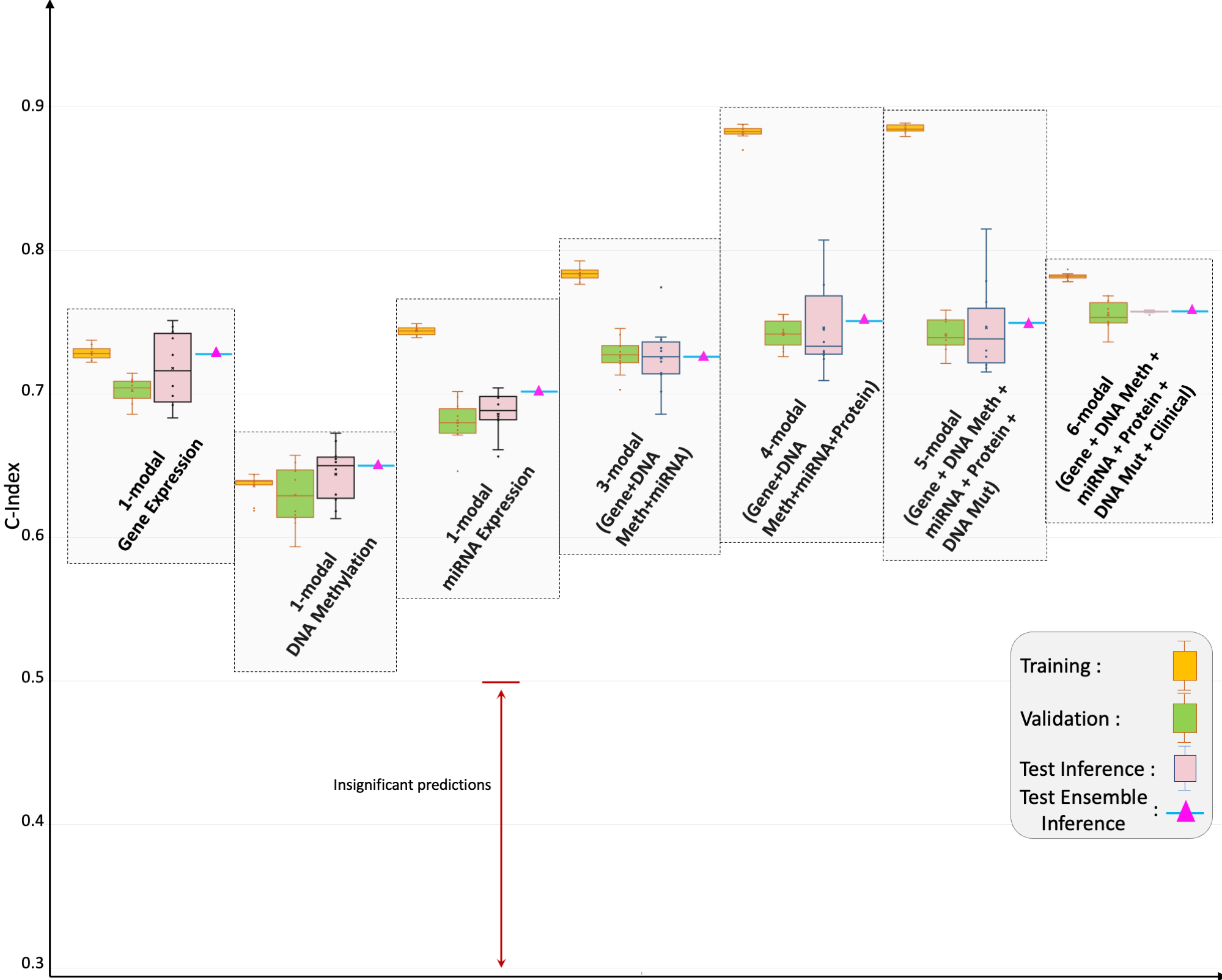
Figure 5: Pan-cancer C-Index results for OS prediction. We trained and evaluated the SeNMo model on different combinations of data modalities. Training and validation was carried out on the $80\%$ of the total data, whereas inference was done on the $20\%$ held-out test set. As the number of modalities increased in the pan-cancer data, the model’s performance improved as depicted by the upward trend of C-Index. All the results shown here are statistically significant, i.e., $p<0.05$.

3 Results

3.1 Pan-Cancer Multimodal Analysis - Overall Survival

For the overall survival (OS) task, the pan-cancer data was randomly divided into the training-validation set ($80\%$) and the held-out test set ($20\%$), for each cancer type. The pan-cancer training was carried out by combining the training-validation cohort of all $33$ cancer types and adopting the 10-fold cross-validation with the $80-20\%$ division of samples. The training-validation cohort has $11,050$ patients, each having $\mathbb{R}^{80,697}$ features, comprised of the six multi-omics modalities including, gene expression, DNA methylation, miRNA expression, protein expression, DNA mutation, and the four clinical features (age, gender, race, stage). The SeNMo encoder model was trained on the training-validation cohort for the regression task of predicting the OS. C-Index was used as the evaluation metric of the hazard score predicted by the model. We used weights and biases [108] to find the optimal set of hyperparameters for our deep learning model. Figure 9 shows the visualization of the parallel sweeps across all hyperparameters, resulting in training around $400$ unique models. The best model had a learning rate of $0.00058$, a weight decay of $0.00598$, $0.1058$ dropout, $256$ batch size, $100$ epochs, and seven hidden layers with neurons in these layers as $[1024,512,256,128,48,48,48]$. The trained model has $83.33$ million trainable parameters. The checkpoints were saved for the best model for each of the $10$ folds. The model’s training resulted in the average training C-Index of $0.78$ and average validation C-Index of $0.76$, across the $10$ folds. For the evaluation of the trained model, the inference data was created by combining the held-out test set from all $33$ cancer types, resulting in $2754$ patients, each having $\mathbb{R}^{80,697}$ features. The inference on the test set showed the C-Index of $0.757$ which was the average of the C-Indices from the $10$ checkpoints. To further validate our findings, we created the ensemble of the $10$ checkpoints by averaging the prediction vectors from all the models and then evaluating the final averaged prediction vector for C-Index. For the pan-cancer, multi-omics SeNMo model, we got the ensemble C-Index of $0.758$ on the held-out test set. The significance level in all these analyses is $95\%$, i.e., $p<0.05$ which indicates statistically significant values. These results are depicted in the Figure 5. We further tested the optimal hyperparameters of our trained model to train different combinations of the pan-cancer data modalities. We call these 1-modal, 3-modal (gene expression, DNA methylation, miRNA expression), 4-modal ($3+$protein expression), 5-modal ($4+$DNA mutation), and 6-modal (all modalities) cohorts. It is important to note that our initially trained pan-cancer, multi-omics model belongs to the 6-modal cohort. The purpose here is to see how the model performs on each of these pan-cancer cohorts where one or more of the data modalities is missing. As depicted in Figure 5, the SeNMo model trained on the pan-cancer 1-modal (Gene expression) cohort showed a C-Index for training, validation, testing, and ensemble inference as $0.729,0.702,0.718,$ and $0.728$, respectively. For the pan-cancer 1-modal (DNA methylation) cohort, the model’s training, validation, testing, and ensemble inference C-indices are $0.636,0.629,0.644,$ and $0.65$, respectively. For the pan-cancer 1-modal (miRNA expression) cohort, the model’s training, validation, testing, and ensemble inference C-indices are $0.744,0.68,0.686,$ and $0.702$, respectively. We did not analyze the model individually on the rest of the three modalities because clinical and protein expression features are too small for an $83$ million-parameter model, whereas the DNA mutation data comprised the binarized features of mutations. Evaluating the model on the 3-modal cohort showed the training, validation, testing, and ensemble inference C-indices of $0.783,0.727,0.725,$ and $0.726$, respectively. Further adding the protein expression to the 3-modal data, we trained and evaluated the model on the 4-modal cohort and got the C-Indices of $0.88,0.742,0.746,$ and $0.751$ for training, validation, testing, and ensemble inference, respectively. Lastly, the model’s performance on the 5-modal cohort showed the training, validation, testing, and ensemble inference C-indices of $0.885,0.741,0.746,$ and $0.749$, respectively. Next, we analyze how the model trained on pan-cancer, 6-modal data fared on individual cancer patients’ data.

3.2 Cancer-wise Multimodal Analysis - Overall Survival

We evaluated the model trained on the 6-modal pan-cancer cohort on the held-out individual cancer data. The number of patients in these cancer cohorts was a randomly selected subset of the cases shown in Figure 3, and Tables 1, 2, which accounts for the $20\%$ of the total samples. The trained model was evaluated on each of the 33 individual cancer data using simple inference as well as the ensemble of the 10-fold checkpoints. Figure 6 shows the evaluation performance of the model on 33 cancer types. The model showed the best predictive performance on TCGA-PCPG data with an average C-Index on the test set of $0.9$ and ensemble inference of $0.929$. SeNMo’s performance on the e cancer types in format $\{TestInference,EnsembleInference\}$ is; TCGA-ACC$=\{0.866,0.861\}$, TCGA-UVM$=\{0.822,0.829\}$, TCGA-LGG$=\{0.821,0.823\}$, TCGA-KICH$=\{0.801,0.807\}$, TCGA-KIRC$=\{0.777,0.776\}$, TCGA-KIRP$=\{0.775,0.778\}$, TCGA-UCEC$=\{0.708,0.713\}$, TCGA-THCA$=\{0.696,0.698\}$, TCGA-SKCM$=\{0.691,0.689\}$, TCGA-BRCA$=\{0.687,0.692\}$, TCGA-CESC$=\{0.676,0.682\}$, TCGA-ESCA$=\{0.650,0.648\}$, TCGA-LUAD$=\{0.647,0.653\}$, TCGA-SARC$=\{0.65,0.658\}$, TCGA-STAD$=\{0.631,0.628\}$, TCGA-LIHC$=\{0.627,0.629\}$, TCGA-BLCA$=\{0.609,0.609\}$, TCGA-MESO$=\{0.599,0.615\}$, TCGA-LUSC$=\{0.588,0.592\}$, TCGA-PAAD$=\{0.597,0.598\}$, TCGA-HNSC$=\{0.583,0.583\}$, TCGA-CHOL$=\{0.574,0.574\}$, TCGA-COAD$=\{0.546,0.542\}$, TCGA-THYM$=\{0.555,0.571\}$, TCGA-UCS$=\{0.514,0.541\}$, TCGA-OV$=\{0.518,0.509\}$, TCGA-GBM$=\{0.495,0.493\}$, TCGA-LAML$=\{0.482,0.485\}$, TCGA-DLBC$=\{0.714,0.619\}$, TCGA-READ$=\{0.55,0.551\}$, TCGA-PRAD$=\{0.304,0.3\}$, TCGA-TGCT$=\{0.123,0.091\}$. We noticed that the results for TCGA-GBM, TCGA-LAML, TCGA-PRAD, and TCGA-TGCT were not statistically significant, i.e., $p>0.05$. So, we fine-tuned the model for these datasets by reducing the learning rate, increasing the weight decay and dropout, and letting the model fine-tune for 10 epochs. Resultantly, the model’s performance increased for TCGA-GBM$=\{0.642,0.650\}$, TCGA-LAML$=\{0.627,0.626\}$, and TCGA-PRAD$=\{0.541,0.542\}$. These improvements are depicted with the green arrows and green boxes in Figure 6. However, the model failed to converge for TCGA-TGCT data and consistently gave insignificant predictions.

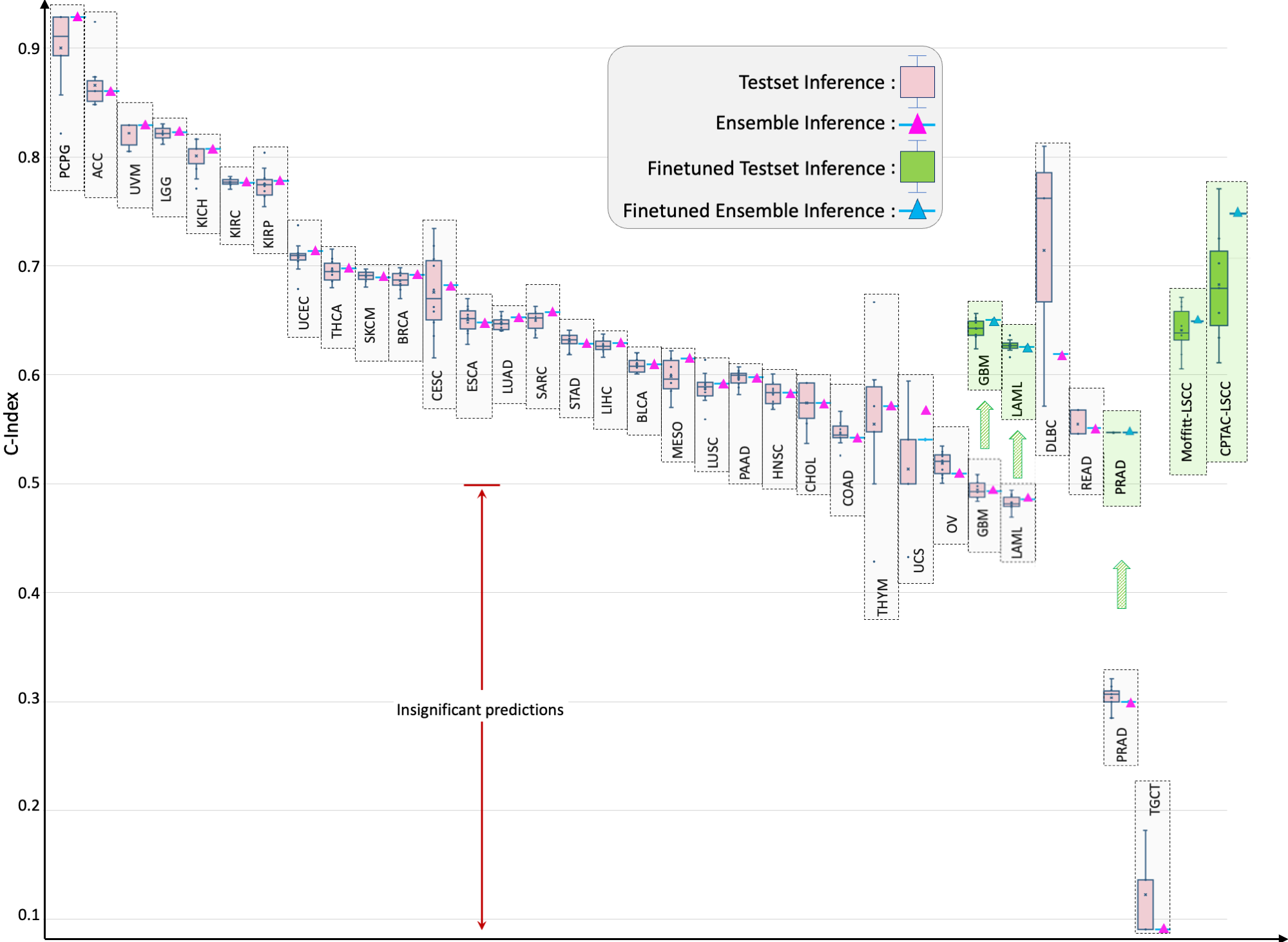
Figure 6: Cancer-wise C-Index results for OS prediction for some of the cancer types.

3.3 Out-of-distribution Evaluation and Fine-tuning

To further verify the performance of our model, we evaluated the model with the off-the-shelf datasets CPTAC-LSCC [56] and Moffitt’s LSCC [57]. These datasets were not part of the training data, depicting the out-of-distribution evaluation. Evaluating the model without fine-tuning showed the $\{TestInference,EnsembleInference\}$ of CPTAC-LSCC$=\{0.48,0.50\}$, and Moffit-LSCC$=\{0.581,0.59\}$. Fine-tuning the model for 10 epochs, with reduced learning rate, and increased weight decay and dropout resulted in the improvement of C-Indices as, CPTAC-LSCC$=\{0.677,0.73\}$, and Moffit-LSCC$=\{0.647,0.656\}$. These fine-tuning results are depicted in Figure 6 as the green box plots.

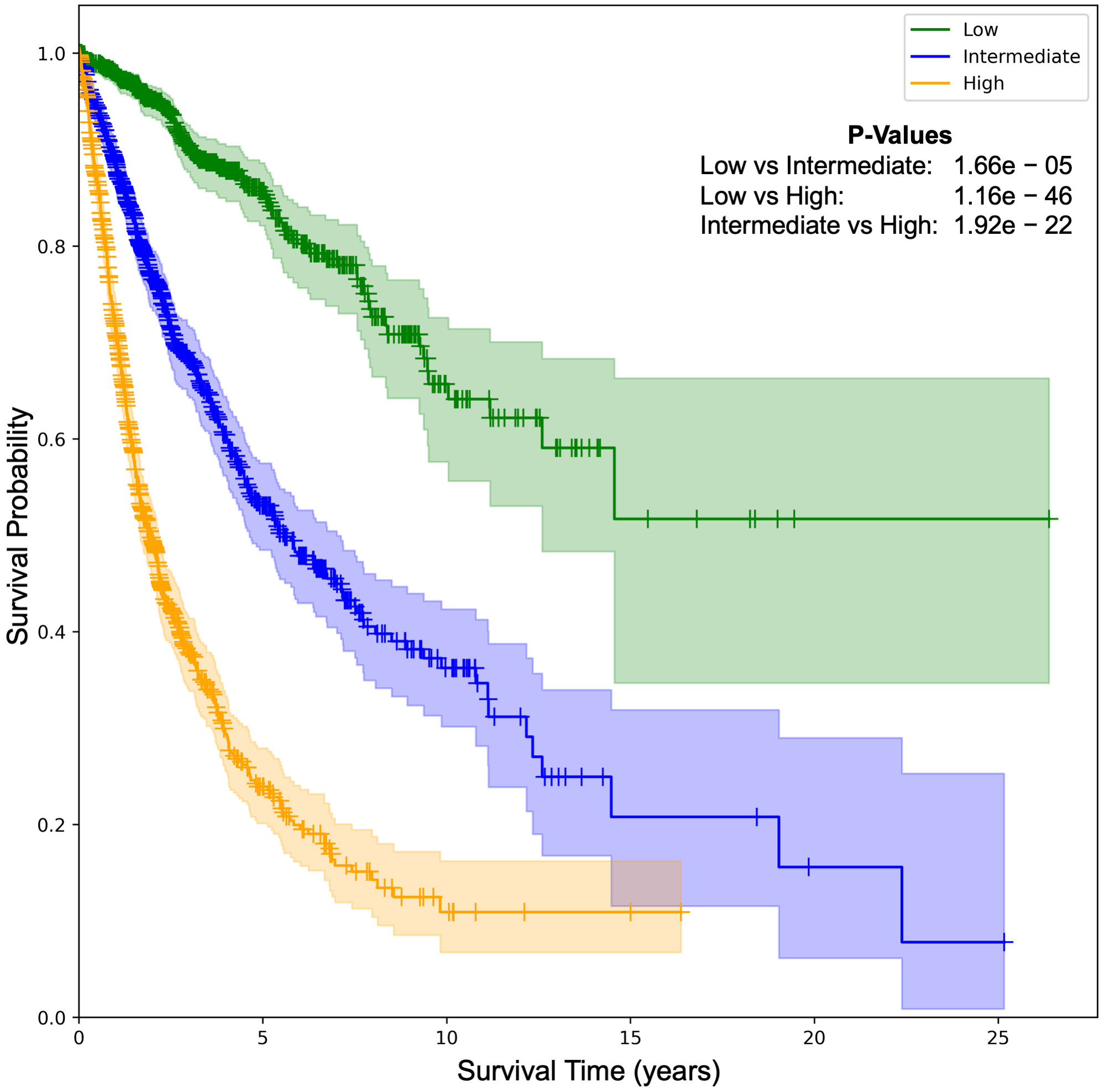
Figure 7: Kaplan-Meier Curves by Risk Group. KM comparative analysis of using SeNMo in stratifying patient outcomes in low/ intermediate/ high risk, defined by the 33-66-100 percentile of hazard predictions. Hazard predictions from SeNMo show clear distinctions between stratified groups. The p-values from logrank test for Low vs. Intermediate: $1.66e-05$, Low vs. High: $1.156e-46$, and Intermediate vs. High: $1.92e-22$. The shaded areas around each curve depicts the 95% confidence intervals.

3.4 Patient Stratification

Risk stratification of patients allows clinicians and researchers to identify patients who might need more intensive care or monitoring and those who may have a better prognosis, facilitating more personalized treatment approaches. We further investigate the SeNMo’s ability to stratify the patients based on low, intermediate, and high risk conditions. We plot Kaplan-Meier (KM) curves of our model on the pan-cancer, multi-omics held-out test set, as shown in Figure 7. We select the low/ intermediate/ high risk stratification distribution as the 33-66-100 percentile of hazard predictions [102, 109]. The hazard scores predicted by SeNMo are used to evaluate the model’s stratification ability. The KM comparative analysis shows that SeNMo distinguished the patients in the three groups across. The low-risk group (green) exhibited the highest survival probability, maintaining close to 100% survival up to approximately 5 years, and gradually declining to about 60% by the 25-year mark. The intermediate-risk group (blue) showed a significantly lower survival probability, starting to diverge from the low-risk group early on and reaching around 40% by the end of the study period. The high-risk group (orange) displayed the most pronounced decline in survival probability, with a steep drop to approximately 20% survival within the first 10 years, and further reducing to below 10% after 10 years. The logrank test to evaluate the significance of this stratification shows that the p-value of low vs. intermediate curves is $1.66e-05$, low vs. high is $1.156e-46$, and intermediate vs. high is $1.92e-22$, showing significant results, i.e., $p<0.05$. The 95% confidence intervals around each curve show the reliability of these estimates.

3.5 Primary Cancer Type Prediction

To test the generalizability of SeNMo across different tasks, we carried out the prediction of primary cancer type from pan-cancer, multi-omics data. We set the problem as a classification problem, where the multi-omics data is used to predict the type of cancer for the given patient data among the 33 classes. It is imperative to mention here that the four clinical features in the initial data contained the cancer stage, as shown in Figure 2 and Table 2. When considering cancer type classification problem, the stage adds a bias in the data because of the staging distribution among different cancers. So, for the cancer classification simulations, we excluded the “stage" feature in the clinical data. As shown in Figure 8, the model achieves near-perfect accuracy levels, with 99.9% average accuracy in training, 99.8% in validation, and consistent performance in both simple and ensemble inference approaches. The confusion matrix depicts a clear concentration of values along the diagonal, indicating a high rate of correct predictions across all cancer types. The scatter plot shows an alignment of predicted labels with true labels along the diagonal line, highlighting the model’s robust predictive accuracy. The classification report across various cancer types reveals that the model consistently maintains high precision, recall, and F1-scores, approaching a value of 1 for almost all categories.

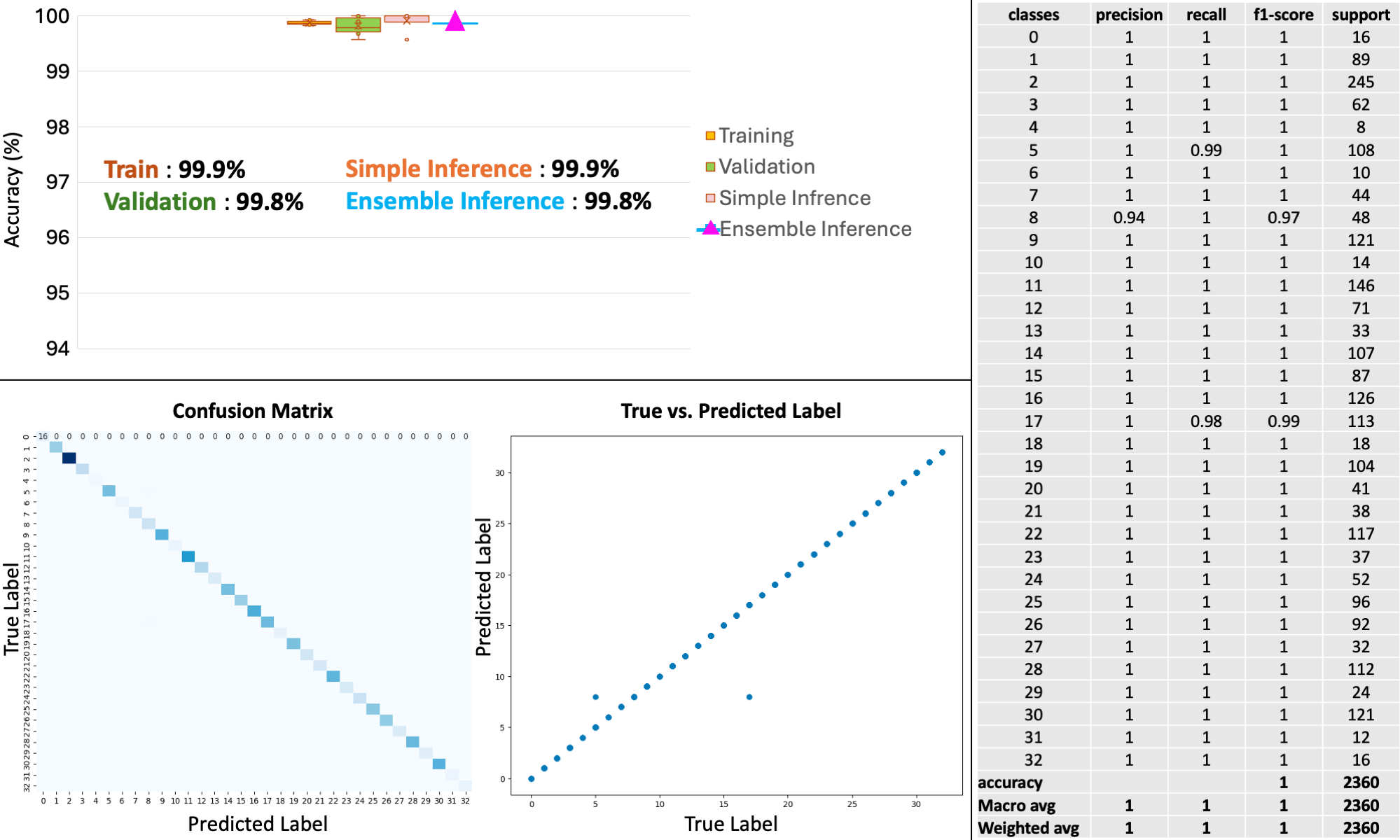
Figure 8: Pan-cancer primary cancer type prediction. The model’s accuracy across training, validation, and inference stages is near-perfect (top left panel). Confusion matrix (bottom left) shows minimal misclassifications, while the scatter plot (bottom middle) shows the alignment of predicted versus true labels. The classification report (right panel) shows high precision, recall, and f1-scores in the 33 cancers type-identification.

4 Discussion and Conclusion

We analyzed pan-cancer dataset of 33 cancer types comprising five molecular data modalities having varying features and four features of clinical data using SeNMo encoder-based framework. In training such a large dataset having high-dimensional heterogeneous data is challenging. Molecular data, such as gene expression, miRNA expression, DNA methylation and mutations, and proteomics, are available from the same patient. This high-dimensional data has intra- and inter-dataset correlations, heterogeneous measurement scales, missing values, technical variations, and other forms of noise [10]. The optimal parameters of a deep learning model that can learn from this data is a non-trivial task. After extensive training-evaluation runs, we found a model that has shown to perform very well across the different data types and tasks, refer to Figures 5 and 9. The model has been shown to outperform the existing works in OS prediction when considering the six data modalities [36]. Moreover, we observe that adding more numbers and types of modalities increased the model’s performance.

The model’s performance was evaluated on individual cancers at test-time through simple inference and ensembling methods. We observed that the model’s predictive power improved when an ensemble of the checkpoints was employed, refer to Figure 6. However, for four data types, TCGA-GBM, TCGA-LAML, TCGA-PRAD, and TCGA-TGCT, the model showed insignificant predictive power. During the investigation, we observed that these datasets had non-admissible pairs in some of the data folds, i.e., all samples had censor value $\delta=0$ in Equation 10. In the case of TCGA-PRAD and TCGA-TGCT, the number of samples having $\delta=1$ in the training/validation cohort was $12$ and $3$, respectively. We fine-tuned the model for these datasets by using the stratified k-folds to offset the class-representation problem in the data folds. After searching for the optimal hyperparameters for fine-tuning, the model’s performance became significant ($p<0.05$) for three out of four datasets, refer to green box plots in Figure 6. The model failed to converge for the TCGA-TGCT data despite numerous efforts at fine-tuning. The authors are of the view that because of the more pronounced class imbalance in this dataset, i.e., 3 out of 111 samples in the training cohort have censor value $\delta=1$, the model cannot learn to distinguish the samples based on the OS.

It is imperative to mention here that MLPs-based networks are very sensitive to catastrophic forgetting when presented with out-of-distribution data or when subjected to a different task [110]. We fine-tuned the SeNMo encoder for one public data (CPTAC-LSCC) and one internal data (Moffitt’s LSCC) [56, 57]. In our simulations to fine-tune the model, we encountered the catastrophic forgetting phenomenon in SeNMo, where the model would fail to converge on these datasets. This was more pronounced when a certain number of hidden layers were frozen, and the rest were trained with lower learning rates, as shown in Figures 10 and 11. We resorted to the option of unfreezing all the layers of the encoder and fine-tuning the model with a very small learning rate ($4e-5$), high weight decay and dropout ($0.35$), and just $10$ epochs. This method worked and the model showed significant performance on the out-of-distribution datasets.

The KM survival curves depicted in Figure 7 demonstrate a clear stratification of survival probabilities among three risk-defined patient groups. These results underscore the effectiveness of the risk stratification model in predicting long-term outcomes and highlight the critical need for targeted therapeutic strategies based on individual risk assessments. This stratification allows for more personalized patient management and could potentially guide clinical decision-making toward improving OS rates across diverse patient populations.

The classification results in Figure 8 illustrate the superior generalizability to the prediction of primary cancer types of the SeNMo encoder, which was primarily trained for predicting OS. Furthermore, the detailed classification report across various cancer types reveals that the model consistently maintains high precision, recall, and F1-scores, for almost all categories. Such metrics not only confirm the model’s effectiveness in accurately identifying the correct cancer class but also its reliability in replicating these results across different samples. This level of performance suggests the capability of the model to handle complex patterns in data.

Data Availability

The molecular data, overall survival information, and other phenotypes from the TCGA and corresponding labels are available from NIH Genomic Data Commons (https://portal.gdc.cancer.gov/). The gene expression, miRNA expression, and DNA Methylation data was obtained from UCSC XENA (https://xena.ucsc.edu/). The CPTAC-LSCC and Moffitt LSCC data are available at [55, 57]. The codebase for the project are available at https://github.com/lab-rasool/SeNMo.

Appendix A1: Hyperparameters Search - Training on Pan-cancer Multiomics Data

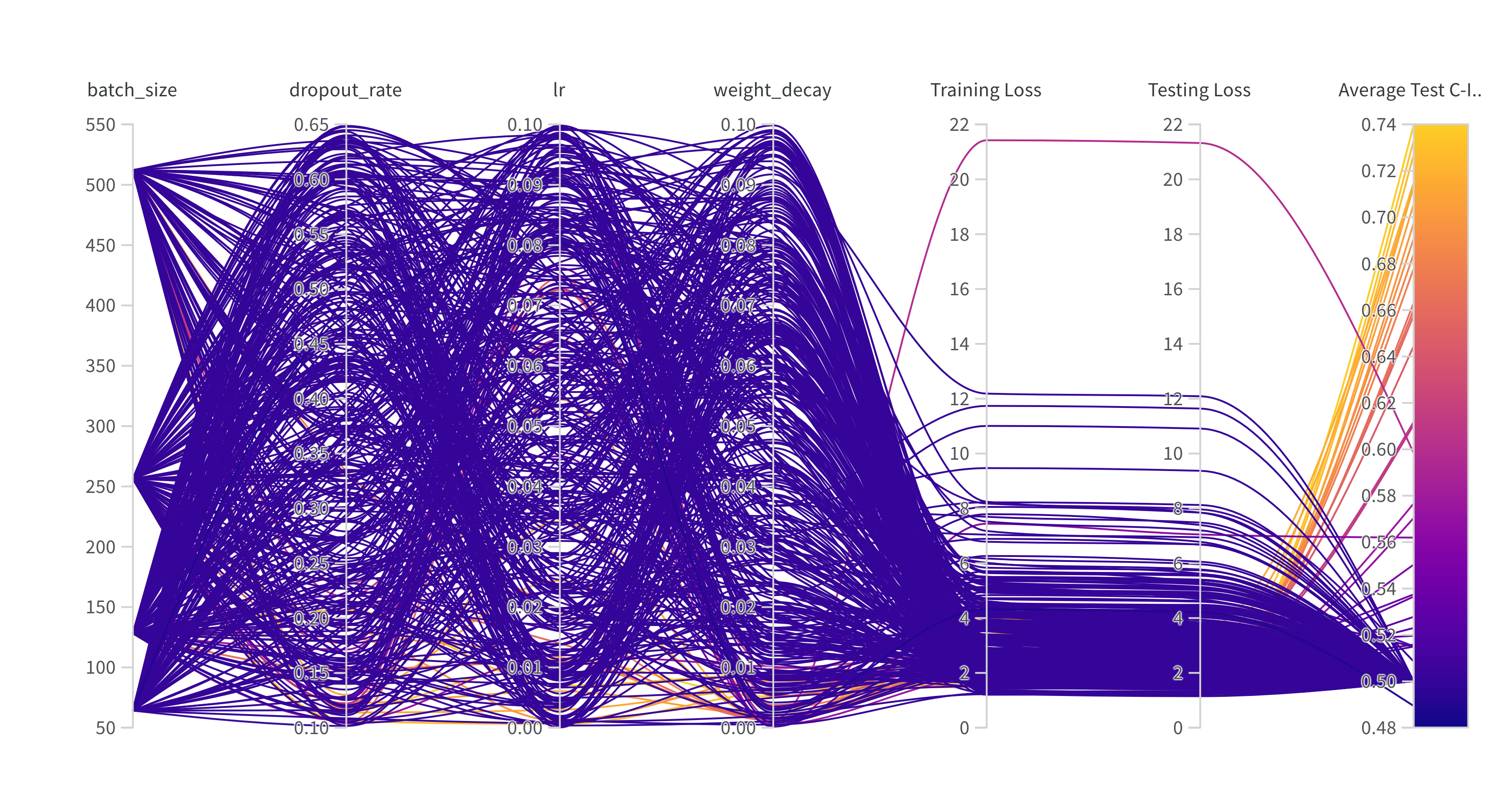
Figure 9: Hyperparameters search for training the SeNMo model on Pan-cancer multiomics data. The goal here was to maximize the validation C-Index.

Appendix A2: Hyperparameters Search - Finetuning CPTAC-LSCC Multiomics Data

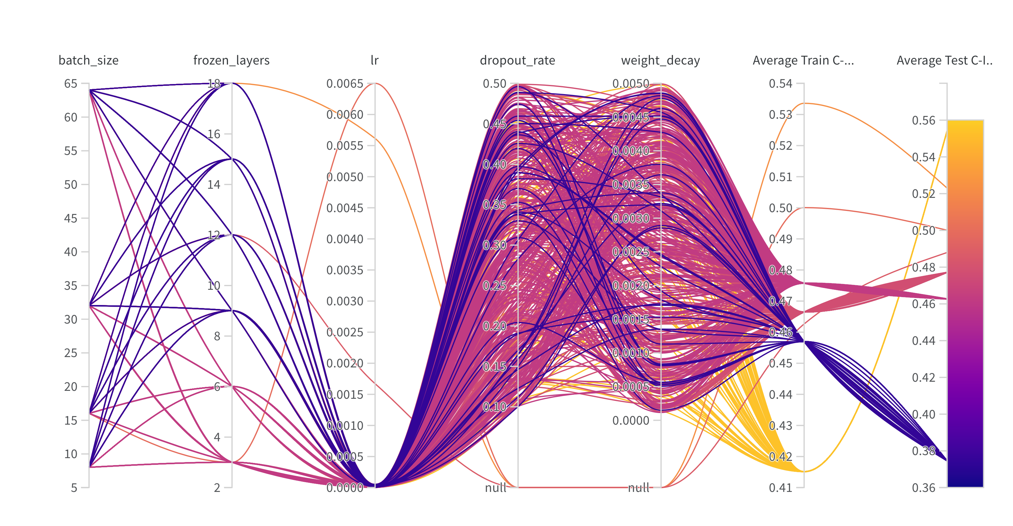
Figure 10: Hyperparameters search for finetuning the SeNMo model on CPTAC-LSCC multiomics data. The goal here was to maximize the validation C-Index.

Appendix A3: Hyperparameters Search - Finetuning Moffitt-SCC Multiomics Data

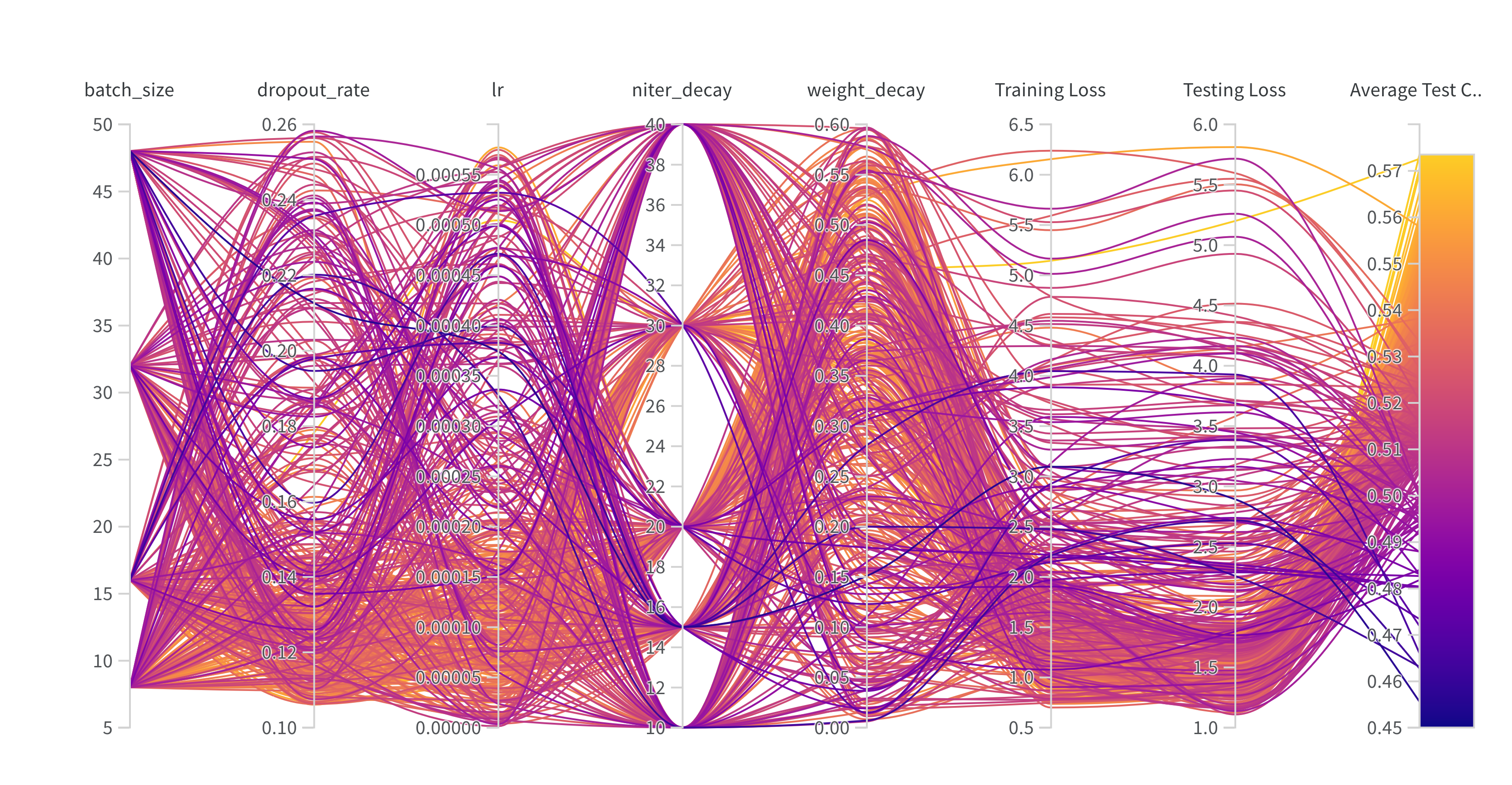
Figure 11: Hyperparameters search for fine-tuning the SeNMo model on Moffitt’s Lung SCC multiomics data. The goal here was to maximize the validation C-Index.

References

- [1] Peng Jiang, Sanju Sinha, Kenneth Aldape, Sridhar Hannenhalli, Cenk Sahinalp, and Eytan Ruppin. Big data in basic and translational cancer research. Nature Reviews Cancer, 22(11):625–639, 2022.
- [2] Kaustav Bera, Nathaniel Braman, Amit Gupta, Vamsidhar Velcheti, and Anant Madabhushi. Predicting cancer outcomes with radiomics and artificial intelligence in radiology. Nature reviews Clinical oncology, 19(2):132–146, 2022.
- [3] R Krithiga and P Geetha. Breast cancer detection, segmentation and classification on histopathology images analysis: a systematic review. Archives of Computational Methods in Engineering, 28(4):2607–2619, 2021.
- [4] Olivier Morin, Martin Vallières, Steve Braunstein, Jorge Barrios Ginart, Taman Upadhaya, Henry C Woodruff, Alex Zwanenburg, Avishek Chatterjee, Javier E Villanueva-Meyer, Gilmer Valdes, et al. An artificial intelligence framework integrating longitudinal electronic health records with real-world data enables continuous pan-cancer prognostication. Nature Cancer, 2(7):709–722, 2021.
- [5] Kasit Chatsirisupachai, Tom Lesluyes, Luminita Paraoan, Peter Van Loo, and João Pedro De Magalhães. An integrative analysis of the age-associated multi-omic landscape across cancers. Nature communications, 12(1):2345, 2021.
- [6] Douglas Hanahan and Robert A Weinberg. Hallmarks of cancer: the next generation. cell, 144(5):646–674, 2011.
- [7] Julián N Acosta, Guido J Falcone, Pranav Rajpurkar, and Eric J Topol. Multimodal biomedical ai. Nature Medicine, 28(9):1773–1784, 2022.
- [8] Dahui Qin. Next-generation sequencing and its clinical application. Cancer biology & medicine, 16(1):4, 2019.
- [9] Asim Waqas, Aakash Tripathi, Ravi P Ramachandran, Paul Stewart, and Ghulam Rasool. Multimodal data integration for oncology in the era of deep neural networks: a review. arXiv preprint arXiv:2303.06471, 2023.
- [10] Zhi Zhao, John Zobolas, Manuela Zucknick, and Tero Aittokallio. Tutorial on survival modeling with applications to omics data. Bioinformatics, page btae132, 2024.
- [11] Yehudit Hasin, Marcus Seldin, and Aldons Lusis. Multi-omics approaches to disease. Genome biology, 18:1–15, 2017.
- [12] Timothy Underwood. Pan-cancer analysis of whole genomes. Nature, 578(7793):82–93, 2020.
- [13] Zheng Hu, Zan Li, Zhicheng Ma, and Christina Curtis. Multi-cancer analysis of clonality and the timing of systemic spread in paired primary tumors and metastases. Nature genetics, 52(7):701–708, 2020.
- [14] Francisco Sanchez-Vega, Marco Mina, Joshua Armenia, Walid K Chatila, Augustin Luna, Konnor C La, Sofia Dimitriadoy, David L Liu, Havish S Kantheti, Sadegh Saghafinia, et al. Oncogenic signaling pathways in the cancer genome atlas. Cell, 173(2):321–337, 2018.
- [15] Katherine A Hoadley, Christina Yau, Toshinori Hinoue, Denise M Wolf, Alexander J Lazar, Esther Drill, Ronglai Shen, Alison M Taylor, Andrew D Cherniack, Vésteinn Thorsson, et al. Cell-of-origin patterns dominate the molecular classification of 10,000 tumors from 33 types of cancer. Cell, 173(2):291–304, 2018.
- [16] Vésteinn Thorsson, David L Gibbs, Scott D Brown, Denise Wolf, Dante S Bortone, Tai-Hsien Ou Yang, Eduard Porta-Pardo, Galen F Gao, Christopher L Plaisier, James A Eddy, et al. The immune landscape of cancer. Immunity, 48(4):812–830, 2018.
- [17] Yize Li, Eduard Porta-Pardo, Collin Tokheim, Matthew H Bailey, Tomer M Yaron, Vasileios Stathias, Yifat Geffen, Kathleen J Imbach, Song Cao, Shankara Anand, et al. Pan-cancer proteogenomics connects oncogenic drivers to functional states. Cell, 186(18):3921–3944, 2023.
- [18] Debabrata Acharya and Anirban Mukhopadhyay. A comprehensive review of machine learning techniques for multi-omics data integration: challenges and applications in precision oncology. Briefings in Functional Genomics, page elae013, 2024.
- [19] Asim Waqas, Dimah Dera, Ghulam Rasool, Nidhal Carla Bouaynaya, and Hassan M Fathallah-Shaykh. Brain tumor segmentation and surveillance with deep artificial neural networks. Deep Learning for Biomedical Data Analysis: Techniques, Approaches, and Applications, pages 311–350, 2021.
- [20] Sabeen Ahmed, Dimah Dera, Saud Ul Hassan, Nidhal Bouaynaya, and Ghulam Rasool. Failure detection in deep neural networks for medical imaging. Frontiers in Medical Technology, 4:919046, 2022.
- [21] Asim Waqas, Hamza Farooq, Nidhal C Bouaynaya, and Ghulam Rasool. Exploring robust architectures for deep artificial neural networks. Communications Engineering, 1(1):46, 2022.
- [22] Jana Lipkova, Richard J Chen, Bowen Chen, Ming Y Lu, Matteo Barbieri, Daniel Shao, Anurag J Vaidya, Chengkuan Chen, Luoting Zhuang, Drew FK Williamson, et al. Artificial intelligence for multimodal data integration in oncology. Cancer cell, 40(10):1095–1110, 2022.
- [23] Kevin M Boehm, Pegah Khosravi, Rami Vanguri, Jianjiong Gao, and Sohrab P Shah. Harnessing multimodal data integration to advance precision oncology. Nature Reviews Cancer, 22(2):114–126, 2022.
- [24] Xiujing He, Xiaowei Liu, Fengli Zuo, Hubing Shi, and Jing Jing. Artificial intelligence-based multi-omics analysis fuels cancer precision medicine. In Seminars in Cancer Biology, volume 88, pages 187–200. Elsevier, 2023.
- [25] Sandra Steyaert, Marija Pizurica, Divya Nagaraj, Priya Khandelwal, Tina Hernandez-Boussard, Andrew J Gentles, and Olivier Gevaert. Multimodal data fusion for cancer biomarker discovery with deep learning. Nature machine intelligence, 5(4):351–362, 2023.
- [26] Asim Waqas, Aakash Tripathi, Ashwin Mukund, Paul Stewart, Mia Naeini, and Ghulam Rasool. Bio24-031: Hierarchical multimodal learning on pan-squamous cell carcinomas for improved survival outcomes. Journal of the National Comprehensive Cancer Network, 22(2.5), 2024.
- [27] Aakash Tripathi, Asim Waqas, Yasin Yilmaz, and Ghulam Rasool. Multimodal transformer model improves survival prediction in lung cancer compared to unimodal approaches. Cancer Research, 84(6_Supplement):4905–4905, 2024.
- [28] Aakash Tripathi, Asim Waqas, Kavya Venkatesan, Yasin Yilmaz, and Ghulam Rasool. Building flexible, scalable, and machine learning-ready multimodal oncology datasets. Sensors, 24(5):1634, 2024.
- [29] Junyi Li, Qingzhe Xu, Mingxiao Wu, Tao Huang, and Yadong Wang. Pan-cancer classification based on self-normalizing neural networks and feature selection. Frontiers in Bioengineering and Biotechnology, 8:766, 2020.
- [30] Richard J Chen, Ming Y Lu, Drew FK Williamson, Tiffany Y Chen, Jana Lipkova, Zahra Noor, Muhammad Shaban, Maha Shady, Mane Williams, Bumjin Joo, et al. Pan-cancer integrative histology-genomic analysis via multimodal deep learning. Cancer Cell, 40(8):865–878, 2022.
- [31] Olivier B Poirion, Zheng Jing, Kumardeep Chaudhary, Sijia Huang, and Lana X Garmire. Deepprog: an ensemble of deep-learning and machine-learning models for prognosis prediction using multi-omics data. Genome medicine, 13:1–15, 2021.
- [32] Seema Khadirnaikar, Sudhanshu Shukla, and SRM Prasanna. Integration of pan-cancer multi-omics data for novel mixed subgroup identification using machine learning methods. Plos one, 18(10):e0287176, 2023.
- [33] Tianle Ma and Aidong Zhang. Integrate multi-omics data with biological interaction networks using multi-view factorization autoencoder (mae). BMC genomics, 20(Suppl 11):944, 2019.
- [34] Ning Zhao, Maozu Guo, Kuanquan Wang, Chunlong Zhang, and Xiaoyan Liu. Identification of pan-cancer prognostic biomarkers through integration of multi-omics data. Frontiers in Bioengineering and Biotechnology, 8:268, 2020.
- [35] Jacob G Ellen, Etai Jacob, Nikos Nikolaou, and Natasha Markuzon. Autoencoder-based multimodal prediction of non-small cell lung cancer survival. Scientific Reports, 13(1):15761, 2023.
- [36] Nikolaos Nikolaou, Domingo Salazar, Harish RaviPrakash, Miguel Goncalves, Rob Mulla, Nikolay Burlutskiy, Natasha Markuzon, and Etai Jacob. Quantifying the advantage of multimodal data fusion for survival prediction in cancer patients. bioRxiv, pages 2024–01, 2024.
- [37] Zhiwei Rong, Zhilin Liu, Jiali Song, Lei Cao, Yipe Yu, Mantang Qiu, and Yan Hou. Mcluster-vaes: an end-to-end variational deep learning-based clustering method for subtype discovery using multi-omics data. Computers in Biology and Medicine, 150:106085, 2022.
- [38] Liangrui Pan, Dazhen Liu, Yutao Dou, Lian Wang, Zhichao Feng, Pengfei Rong, Liwen Xu, and Shaoliang Peng. Multi-head attention mechanism learning for cancer new subtypes and treatment based on cancer multi-omics data. arXiv preprint arXiv:2307.04075, 2023.
- [39] Weikuan Jia, Meili Sun, Jian Lian, and Sujuan Hou. Feature dimensionality reduction: a review. Complex & Intelligent Systems, 8(3):2663–2693, 2022.
- [40] Jerzy Krawczuk and Tomasz Łukaszuk. The feature selection bias problem in relation to high-dimensional gene data. Artificial intelligence in medicine, 66:63–71, 2016.
- [41] Shuai Yang, Xianjie Guo, Kui Yu, Xiaoling Huang, Tingting Jiang, Jin He, and Lichuan Gu. Causal feature selection in the presence of sample selection bias. ACM Transactions on Intelligent Systems and Technology, 14(5):1–18, 2023.
- [42] Asim Waqas, Marilyn M Bui, Eric F Glassy, Issam El Naqa, Piotr Borkowski, Andrew A Borkowski, and Ghulam Rasool. Revolutionizing digital pathology with the power of generative artificial intelligence and foundation models. Laboratory Investigation, page 100255, 2023.
- [43] Tom Brown, Benjamin Mann, Nick Ryder, Melanie Subbiah, Jared D Kaplan, Prafulla Dhariwal, Arvind Neelakantan, Pranav Shyam, Girish Sastry, Amanda Askell, et al. Language models are few-shot learners. Advances in neural information processing systems, 33:1877–1901, 2020.
- [44] Jacob Devlin, Ming-Wei Chang, Kenton Lee, and Kristina Toutanova. Bert: Pre-training of deep bidirectional transformers for language understanding. arXiv preprint arXiv:1810.04805, 2018.
- [45] Iryna Hartsock and Ghulam Rasool. Vision-language models for medical report generation and visual question answering: A review. arXiv preprint arXiv:2403.02469, 2024.
- [46] Alec Radford, Jong Wook Kim, Chris Hallacy, Aditya Ramesh, Gabriel Goh, Sandhini Agarwal, Girish Sastry, Amanda Askell, Pamela Mishkin, Jack Clark, et al. Learning transferable visual models from natural language supervision. In International conference on machine learning, pages 8748–8763. PMLR, 2021.
- [47] Jiasen Lu, Dhruv Batra, Devi Parikh, and Stefan Lee. Vilbert: Pretraining task-agnostic visiolinguistic representations for vision-and-language tasks. Advances in neural information processing systems, 32, 2019.
- [48] Katarzyna Tomczak, Patrycja Czerwińska, and Maciej Wiznerowicz. Review The Cancer Genome Atlas (TCGA): An immeasurable source of knowledge. Contemporary Oncology, 2015(1):68–77, 2015.
- [49] Matthew J. Ellis, Michael Gillette, Steven A. Carr, Amanda G. Paulovich, Richard D. Smith, Karin K. Rodland, R. Reid Townsend, Christopher Kinsinger, Mehdi Mesri, Henry Rodriguez, and Daniel C. Liebler. Connecting Genomic Alterations to Cancer Biology with Proteomics: The NCI Clinical Proteomic Tumor Analysis Consortium. Cancer Discovery, 3(10):1108–1112, 10 2013.
- [50] Haotian Cui, Chloe Wang, Hassaan Maan, Kuan Pang, Fengning Luo, Nan Duan, and Bo Wang. scgpt: toward building a foundation model for single-cell multi-omics using generative ai. Nature Methods, pages 1–11, 2024.
- [51] Wen Zhu, Yiwen Chen, Shanling Nie, and Hai Yang. Samms: Multi-modality deep learning with the foundation model for the prediction of cancer patient survival. In 2023 IEEE International Conference on Bioinformatics and Biomedicine (BIBM), pages 3662–3668. IEEE, 2023.
- [52] Jiayang Chen, Zhihang Hu, Siqi Sun, Qingxiong Tan, Yixuan Wang, Qinze Yu, Licheng Zong, Liang Hong, Jin Xiao, Tao Shen, et al. Interpretable rna foundation model from unannotated data for highly accurate rna structure and function predictions. arXiv preprint arXiv:2204.00300, 2022.
- [53] Hongxiao Wang, Yang Yang, Zhuo Zhao, Pengfei Gu, Nishchal Sapkota, and Danny Z Chen. Path-gptomic: A balanced multi-modal learning framework for survival outcome prediction. arXiv preprint arXiv:2403.11375, 2024.
- [54] Saghir Alfasly, Peyman Nejat, Sobhan Hemati, Jibran Khan, Isaiah Lahr, Areej Alsaafin, Abubakr Shafique, Nneka Comfere, Dennis Murphree, Chady Meroueh, et al. When is a foundation model a foundation model. arXiv preprint arXiv:2309.11510, 2023.
- [55] Mary Goldman, Brian Craft, Mim Hastie, Kristupas Repečka, Fran McDade, Akhil Kamath, Ayan Banerjee, Yunhai Luo, Dave Rogers, Angela N Brooks, et al. The ucsc xena platform for public and private cancer genomics data visualization and interpretation. biorxiv, page 326470, 2018.
- [56] Shankha Satpathy, Karsten Krug, Pierre M Jean Beltran, Sara R Savage, Francesca Petralia, Chandan Kumar-Sinha, Yongchao Dou, Boris Reva, M Harry Kane, Shayan C Avanessian, et al. A proteogenomic portrait of lung squamous cell carcinoma. Cell, 184(16):4348–4371, 2021.
- [57] Paul A Stewart, Eric A Welsh, Robbert JC Slebos, Bin Fang, Victoria Izumi, Matthew Chambers, Guolin Zhang, Ling Cen, Fredrik Pettersson, Yonghong Zhang, et al. Proteogenomic landscape of squamous cell lung cancer. Nature communications, 10(1):3578, 2019.
- [58] Virinder Kaur Sarhadi and Gemma Armengol. Molecular biomarkers in cancer. Biomolecules, 12(8):1021, 2022.
- [59] Feng Chen, Michael C Wendl, Matthew A Wyczalkowski, Matthew H Bailey, Yize Li, and Li Ding. Moving pan-cancer studies from basic research toward the clinic. Nature cancer, 2(9):879–890, 2021.
- [60] Netanel Loyfer, Judith Magenheim, Ayelet Peretz, Gordon Cann, Joerg Bredno, Agnes Klochendler, Ilana Fox-Fisher, Sapir Shabi-Porat, Merav Hecht, Tsuria Pelet, et al. A dna methylation atlas of normal human cell types. Nature, 613(7943):355–364, 2023.
- [61] Ranjani Lakshminarasimhan and Gangning Liang. The role of dna methylation in cancer. DNA Methyltransferases-Role and Function, pages 151–172, 2016.
- [62] Pan Du, Xiao Zhang, Chiang-Ching Huang, Nadereh Jafari, Warren A Kibbe, Lifang Hou, and Simon M Lin. Comparison of beta-value and m-value methods for quantifying methylation levels by microarray analysis. BMC bioinformatics, 11:1–9, 2010.
- [63] Zhenxing Wang, XiaoLiang Wu, and Yadong Wang. A framework for analyzing dna methylation data from illumina infinium humanmethylation450 beadchip. BMC bioinformatics, 19:15–22, 2018.
- [64] Luis A Corchete, Elizabeta A Rojas, Diego Alonso-López, Javier De Las Rivas, Norma C Gutiérrez, and Francisco J Burguillo. Systematic comparison and assessment of rna-seq procedures for gene expression quantitative analysis. Scientific reports, 10(1):19737, 2020.
- [65] Sara Hijazo-Pechero, Ania Alay, Raúl Marín, Noelia Vilariño, Cristina Muñoz-Pinedo, Alberto Villanueva, David Santamaría, Ernest Nadal, and Xavier Solé. Gene expression profiling as a potential tool for precision oncology in non-small cell lung cancer. Cancers, 13(19):4734, 2021.
- [66] Augusto Gonzalez, Dario A Leon, Yasser Perera, and Rolando Perez. On the gene expression landscape of cancer. Plos one, 18(2):e0277786, 2023.
- [67] Andrea Rau, Michael Flister, Hallgeir Rui, and Paul L Auer. Exploring drivers of gene expression in the cancer genome atlas. Bioinformatics, 35(1):62–68, 2019.
- [68] EBI Gene Expression Team. Expression atlas. https://www.ebi.ac.uk/gxa/FAQ.html/. Accessed: 2024-05-13.
- [69] Yong Peng and Carlo M Croce. The role of micrornas in human cancer. Signal transduction and targeted therapy, 1(1):1–9, 2016.
- [70] Andy Chu, Gordon Robertson, Denise Brooks, Andrew J Mungall, Inanc Birol, Robin Coope, Yussanne Ma, Steven Jones, and Marco A Marra. Large-scale profiling of micrornas for the cancer genome atlas. Nucleic acids research, 44(1):e3–e3, 2016.
- [71] Shuting Lin, Jie Zhou, Yiqiong Xiao, Bridget Neary, Yong Teng, and Peng Qiu. Integrative analysis of tcga data identifies mirnas as drug-specific survival biomarkers. Scientific Reports, 12(1):6785, 2022.
- [72] GDC Documentation. Reverse phase protein array. https://docs.gdc.cancer.gov/Data/Bioinformatics_Pipelines/RPPA_intro/, 2024. Accessed: 2024-05-13.
- [73] MD Anderson. Rppa description. https://www.mdanderson.org/documents/core-facilities/FunctionalProteomicsRPPACoreFacility/RPPADescription_2016.pdf, 2024. Accessed: 2024-05-13.
- [74] Mei-Ju May Chen, Jun Li, Yumeng Wang, Rehan Akbani, Yiling Lu, Gordon B Mills, and Han Liang. Tcpa v3. 0: an integrative platform to explore the pan-cancer analysis of functional proteomic data. Molecular & Cellular Proteomics, 18(8):S15–S25, 2019.
- [75] Jun Li, Yiling Lu, Rehan Akbani, Zhenlin Ju, Paul L Roebuck, Wenbin Liu, Ji-Yeon Yang, Bradley M Broom, Roeland GW Verhaak, David W Kane, et al. Tcpa: a resource for cancer functional proteomics data. Nature methods, 10(11):1046–1047, 2013.
- [76] Zhenlin Ju, Wenbin Liu, Paul L Roebuck, Doris R Siwak, Nianxiang Zhang, Yiling Lu, Michael A Davies, Rehan Akbani, John N Weinstein, Gordon B Mills, et al. Development of a robust classifier for quality control of reverse-phase protein arrays. Bioinformatics, 31(6):912–918, 2015.
- [77] Genomic Data Commons. Mutation annotation format. https://docs.gdc.cancer.gov/Encyclopedia/pages/Mutation_Annotation_Format//#:~:text=MAF%20files%20are%20generated%20at low%20quality%20or%20germline%20mutations, 2024. Accessed: 2024-05-13.
- [78] Genomic Data Commons. File format - vcf. https://docs.gdc.cancer.gov/Data/File_Formats/VCF_Format/, 2024. Accessed: 2024-05-13.
- [79] Genomic Data Commons. File format - maf. https://docs.gdc.cancer.gov/Data/File_Formats/MAF_Format/, 2024. Accessed: 2024-05-13.
- [80] Gaurav Mendiratta, Eugene Ke, Meraj Aziz, David Liarakos, Melinda Tong, and Edward C Stites. Cancer gene mutation frequencies for the us population. Nature communications, 12(1):5961, 2021.
- [81] Michael R Waarts, Aaron J Stonestrom, Young C Park, Ross L Levine, et al. Targeting mutations in cancer. The Journal of clinical investigation, 132(8), 2022.
- [82] Anna Lewandowska, Grzegorz Rudzki, Tomasz Lewandowski, Aleksandra Stryjkowska-Gora, and Sławomir Rudzki. Risk factors for the diagnosis of colorectal cancer. Cancer Control, 29:10732748211056692, 2022.
- [83] Camila M Lopes-Ramos, John Quackenbush, and Dawn L DeMeo. Genome-wide sex and gender differences in cancer. Frontiers in oncology, 10:597788, 2020.
- [84] Valentina A Zavala, Paige M Bracci, John M Carethers, Luis Carvajal-Carmona, Nicole B Coggins, Marcia R Cruz-Correa, Melissa Davis, Adam J de Smith, Julie Dutil, Jane C Figueiredo, et al. Cancer health disparities in racial/ethnic minorities in the united states. British journal of cancer, 124(2):315–332, 2021.
- [85] Xinyu Yang, Dongmei Mu, Hao Peng, Hua Li, Ying Wang, Ping Wang, Yue Wang, and Siqi Han. Research and application of artificial intelligence based on electronic health records of patients with cancer: systematic review. JMIR Medical Informatics, 10(4):e33799, 2022.
- [86] Yingdong Zhao, Ming-Chung Li, Mariam M Konaté, Li Chen, Biswajit Das, Chris Karlovich, P Mickey Williams, Yvonne A Evrard, James H Doroshow, and Lisa M McShane. Tpm, fpkm, or normalized counts? a comparative study of quantification measures for the analysis of rna-seq data from the nci patient-derived models repository. Journal of translational medicine, 19(1):269, 2021.
- [87] Poorvi Kaushik, Evan J Molinelli, Martin L Miller, Weiqing Wang, Anil Korkut, Wenbin Liu, Zhenlin Ju, Yiling Lu, Gordon Mills, and Chris Sander. Spatial normalization of reverse phase protein array data. PloS one, 9(12):e97213, 2014.
- [88] Wenbin Liu, Zhenlin Ju, Yiling Lu, Gordon B Mills, and Rehan Akbani. A comprehensive comparison of normalization methods for loading control and variance stabilization of reverse-phase protein array data. Cancer informatics, 13:CIN–S13329, 2014.
- [89] Meng Song, Jonathan Greenbaum, Joseph Luttrell IV, Weihua Zhou, Chong Wu, Hui Shen, Ping Gong, Chaoyang Zhang, and Hong-Wen Deng. A review of integrative imputation for multi-omics datasets. Frontiers in Genetics, 11:570255, 2020.
- [90] F Anowar, S Sadaoui, and B Selim. Conceptual and empirical comparison of dimensionality reduction algorithms (pca, kpca, lda, mds, svd, lle, isomap, le, ica, t-sne), comput. sci. rev., 40, 100378. ISI, 2021.
- [91] Marzia Settino and Mario Cannataro. Survey of main tools for querying and analyzing tcga data. In 2018 IEEE International Conference on Bioinformatics and Biomedicine (BIBM), pages 1711–1718. IEEE, 2018.
- [92] Brian Lei, Xinyin Jiang, and Anjana Saxena. Tcga expression analyses of 10 carcinoma types reveal clinically significant racial differences. Cancers, 15(10):2695, 2023.
- [93] Feature-engine, a python library for feature engineering and selection. https://feature-engine.trainindata.com/en/latest/index.html. Accessed: 2024-05-13.
- [94] Andrea Bommert, Thomas Welchowski, Matthias Schmid, and Jörg Rahnenführer. Benchmark of filter methods for feature selection in high-dimensional gene expression survival data. Briefings in Bioinformatics, 23(1):bbab354, 2022.
- [95] F. Pedregosa, G. Varoquaux, A. Gramfort, V. Michel, B. Thirion, O. Grisel, M. Blondel, P. Prettenhofer, R. Weiss, V. Dubourg, J. Vanderplas, A. Passos, D. Cournapeau, M. Brucher, M. Perrot, and E. Duchesnay. Scikit-learn: Machine learning in Python. Journal of Machine Learning Research, 12:2825–2830, 2011.
- [96] Giacomo Baruzzo, Ilaria Patuzzi, and Barbara Di Camillo. Beware to ignore the rare: how imputing zero-values can improve the quality of 16s rrna gene studies results. BMC bioinformatics, 22(Suppl 15):618, 2021.
- [97] Fetty Tri Anggraeny, Intan Yuniar Purbasari, M Syahrul Munir, Faisal Muttaqin, Eka Prakarsa Mandyarta, and Fawwaz Ali Akbar. Analysis of simple data imputation in disease dataset. In International Conference on Science and Technology (ICST 2018), pages 471–475. Atlantis Press, 2018.
- [98] Tomas Rakvåg Ulriksborg. Imputation of missing time series values using statistical and mathematical strategies. Department of Informatics, 2022.
- [99] Yin Zheng, Bangsheng Tang, Wenkui Ding, and Hanning Zhou. A neural autoregressive approach to collaborative filtering. In International Conference on Machine Learning, pages 764–773. PMLR, 2016.
- [100] Divyanshu Talwar, Aanchal Mongia, Debarka Sengupta, and Angshul Majumdar. Autoimpute: Autoencoder based imputation of single-cell rna-seq data. Scientific reports, 8(1):16329, 2018.
- [101] Joonyoung Yi, Juhyuk Lee, Kwang Joon Kim, Sung Ju Hwang, and Eunho Yang. Why not to use zero imputation? correcting sparsity bias in training neural networks. arXiv preprint arXiv:1906.00150, 2019.
- [102] Richard J Chen, Ming Y Lu, Jingwen Wang, Drew FK Williamson, Scott J Rodig, Neal I Lindeman, and Faisal Mahmood. Pathomic fusion: an integrated framework for fusing histopathology and genomic features for cancer diagnosis and prognosis. IEEE Transactions on Medical Imaging, 41(4):757–770, 2020.
- [103] Kedar A Patwardhan, Harish RaviPrakash, Nikos Nikolaou, Ignacio Gonzalez-Garcia, Jose Domingo Salazar, Paul Metcalfe, and Joachim Reischl. Towards a survival risk prediction model for metastatic nsclc patients on durvalumab using whole-lung ct radiomics. bioRxiv, pages 2024–02, 2024.
- [104] Kimberly D Miller, Leticia Nogueira, Angela B Mariotto, Julia H Rowland, K Robin Yabroff, Catherine M Alfano, Ahmedin Jemal, Joan L Kramer, and Rebecca L Siegel. Cancer treatment and survivorship statistics, 2019. CA: a cancer journal for clinicians, 69(5):363–385, 2019.
- [105] Günter Klambauer, Thomas Unterthiner, Andreas Mayr, and Sepp Hochreiter. Self-normalizing neural networks. Advances in neural information processing systems, 30, 2017.
- [106] Travers Ching. Cox regression. http://traversc.github.io/cox-nnet/docs/, 2024. Accessed: 2024-05-13.
- [107] Cameron Davidson-Pilon. lifelines, survival analysis in python. https://doi.org/10.5281/zenodo.10456828, Jan 2024. Accessed: 2024-05-13.
- [108] Lukas Biewald. Experiment tracking with weights and biases, 2020. Software available from wandb.com.
- [109] Zhe Li, Yuming Jiang, Mengkang Lu, Ruijiang Li, and Yong Xia. Survival prediction via hierarchical multimodal co-attention transformer: A computational histology-radiology solution. IEEE Transactions on Medical Imaging, 2023.
- [110] Ziming Liu, Yixuan Wang, Sachin Vaidya, Fabian Ruehle, James Halverson, Marin Soljačić, Thomas Y Hou, and Max Tegmark. Kan: Kolmogorov-arnold networks. arXiv preprint arXiv:2404.19756, 2024.