Random Utility Models with Skewed Random Components:
the Smallest versus Largest Extreme Value Distribution

Abstract

At the core of most random utility models (RUMs) involving multinomial choice behavior is an individual agent with a random utility component following a largest extreme value Type I (LEVI) distribution. What if, instead, the random component follows its mirror image — the smallest extreme value Type I (SEVI) distribution? Differences between these specifications, closely tied to the random component’s skewness, can be quite profound. For the same preference parameters, the two RUMs, equivalent with only two choice alternatives, diverge progressively as the number of alternatives increases, resulting in substantially different estimates and predictions for key measures, such as elasticities and market shares.

The LEVI model imposes the well-known independence-of-irrelevant-alternatives property, while SEVI does not. Instead, the SEVI choice probability for a particular option involves enumerating all subsets that contain this option. The SEVI model, though more complex to estimate, is shown to have computationally tractable closed-form choice probabilities. Much of the paper delves into explicating the properties of the SEVI model and exploring implications of the random component’s skewness, including offering new insights into multinomial probit models. SEVI-based counterparts exist for most LEVI-based generalizations of the conditional logit model such as mixed logit, and the LEVI versus SEVI issue is largely orthogonal to the issues these models are intended to address.

Conceptually, the difference between the LEVI and SEVI models centers on whether information, known only to the agent, is more likely to increase or decrease the systematic utility parameterized using observed attributes. LEVI does the former; SEVI the latter. An immediate implication is that if choice is characterized by SEVI random components, then the observed choice is more likely to correspond to the systematic-utility-maximizing choice than if characterized by LEVI. Examining standard empirical examples from different applied areas, we find that the SEVI model outperforms the LEVI model, suggesting the relevance of its inclusion in applied researchers’ toolkits.

Keywords: Conditional Logit, Gumbel Distribution, Independence of Irrelevant Alternatives, Multinomial Logit, Reverse Gumbel Distribution, Largest Extreme Value Type I Distribution, Smallest Extreme Value Type I Distribution.

JEL codes: C10, C18, C25

1 Introduction

Random utility models (RUM) are a cornerstone of applied microeconomics and other fields such as marketing, health policy, and transportation research. Since the seminal work of McFadden, (1973), the vast majority of RUMs have been formulated as conditional or multinomial logit models, or their generalizations (Hensher et al., (2015) and Train, (2009)). These models posit that the total utility of an alternative comprises two components: a systematic component parameterized by observable attributes, and an idiosyncratic component known only to the agent (Manski, (1977)). The latter is often referred to as the random component, since it is unknown to the econometrician, who generally assumes it follows a specific distribution. The agent chooses the alternative with the highest total utility, making choice behavior appear random from the econometrician’s perspective, even though it may be regarded as deterministic from the agent’s viewpoint.

The conditional logit model and its standard generalizations assume that the random component follows the Largest Extreme Value Type I (LEVI) distribution, also known as the Gumbel or double exponential distribution (Gumbel, (1958)). This distribution is continuous, has a single mode, is asymmetric and skewed with a long right tail. Mirroring the LEVI distribution is the Smallest Extreme Value Type I (SEVI) distribution, also known as the Reverse Gumbel. It is also asymmetric but with a long left tail. This paper presents a systematic study of RUMs based on the SEVI distribution, highlighting their differences from conventional logit models and practical implications.

The natural question at this point for a choice modeler is: does the choice between LEVI and SEVI random components matter empirically? Two important bits of information suggest it should not. First, the difference between two (standard) LEVI random variables or two (standard) SEVI random variables is the same (standard) logistic distribution, and thus, RUMs based on LEVI and SEVI random components are equivalent when there are only two alternatives. Second, there is a long standing belief (Hausman and Wise, (1977); Horowitz, (1982)) that a multinomial probit (MNP) model produces essentially the same results as the conditional/multinomial logit model. This belief has been taken to suggest that it is the iid assumption imposed on the random components that drives the well-known independence of irrelevant alternatives (IIA) substitution pattern. However, insights from the case with only two alternatives do not extend to the case with more than two alternatives. In this paper, we show that as the number of alternatives increases, the choice probabilities from a LEVI-based conditional logit and a SEVI-based conditional logit model increasingly diverge from each other. We also show that the IIA property does not follow from the iid assumption. Even though the random components are still iid, a SEVI-based conditional logit model with more than two alternatives exhibits a distinctly non-IIA substitution pattern.

Let’s consider a simple stylized example. An agent (individual $i$) enters a store with the intention of purchasing a pair of running shoes, and there are five different alternatives $(j\in\{1,2,3,4,5\}$ and $J=5)$ to choose from. Before trying them on, the individual rates each of the five pairs based on observable features like brand and price. These ratings capture the systematic components, $\left\{V_{j}\right\}$, of a random utility model. For illustrative purposes, assume that the $V_{j}$’s are known to be $\{0.25,0.50,0.75,1.50,$ and $2.00\},$ so there is no need to specify the shoe attributes and the associated preference parameters. Next, the individual tries on each of the five pairs of shoes, making an idiosyncratic judgement on comfort and fit. This provides the random component, $\varepsilon_{ij}$, to add to the systematic component, $V_{j}$, to get the total utility level, $U_{ij}=V_{j}+\varepsilon_{ij},$ for each pair of shoes. The chosen pair for purchase is the one with the highest $U_{ij}$.

Now let the store’s customers comprise of a large number of individuals ($i=1,\ldots,n$), with identical and known systematic components $\left\{V_{j}\right\}_{j=1}^{5}$, but different random components $\varepsilon_{ij}.$ They try on the shoes, therefore observing their individual random components, then make their decision on which of the five pairs of shoes to purchase. The question we posed can now be framed solely in terms of: what are the choice probabilities cast in percentage terms (or equivalently, market shares) for each of the five pairs of shoes, if the $\varepsilon_{ij}$ are drawn from the following distributions: (a) the standard LEVI distribution, (b) the standard SEVI distribution, (c) N$(0,\pi^{2}/6)$ (hereafter referred to as NORM, a normal distribution normalized to have the same variance as the standard LEVI and SEVI distributions)?

The answer to this question is displayed in Figure 1. The results are quite striking, particularly for the alternatives with the smallest and largest systematic utilities. With a LEVI error component, the alternative with the smallest systematic utility has a market share 137% higher than its SEVI counterpart and 25% higher than its independent normal counterpart. This pattern continues for the alternatives with the second smallest and third smallest systematic utilities, with LEVI giving rise to market shares 73% and 37% higher than SEVI, respectively. However, this pattern of a higher LEVI market share reverses around a 20% market share (i.e., $1/J$ or equal share for all alternatives), where the SEVI distribution leads to a higher market share than the LEVI distribution. For the alternative with the second-largest systematic utility, the SEVI market share is 11% higher than its LEVI counterpart and 5% higher than that under the NORM distribution. The pattern of a higher market share under SEVI intensifies for the alternative with the largest systematic utility. Here, SEVI leads to a market share 21% higher than LEVI and 16% higher than NORM.

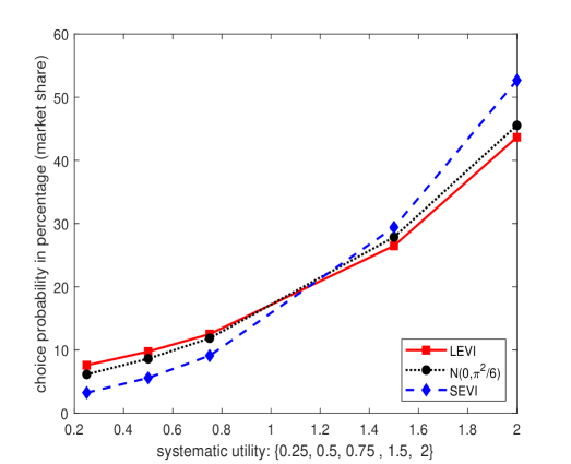
Figure 1: Market shares for all five alternatives in an RUM with identical systematic utilities but different distributions of the random utility components

The magnitude of all of these differences is likely to be important in empirical applications. For instance, if Alternative 1 were a new product, use of a LEVI-based prediction when the true error component was SEVI would have led to an overestimation of demand by more than double (7.6% vs. 3.2% market shares). The potential for the random component to be SEVI rather than LEVI provides one possible explanation for why most new products perform much worse than predicted by marketing researchers. On the other hand, a LEVI-based prediction for the market leader, when the true error component is SEVI, could substantially underestimate its market share (43.7% vs. 52.7%). It is easy to see how either of these faulty predictions could be disastrous from both production and profit perspectives. Antitrust implications are also obvious.

Why do these differences in choice probabilities arise, despite these three simple models sharing the same (known) systematic components and random components from iid draws from simple, single-peaked distributions with the same finite variance? The answer lies in the skewness of the random components. From the econometrician’s viewpoint, the fundamental question in our stylized example is: for a randomly chosen agent, is the overall utility from a randomly chosen pair of shoes (a) more likely to move up, (b) stay the same, or (c) move down? Surprisingly, this fundamental property of the random component of a RUM seems to have never been raised in the voluminous literature on multinomial choice models and serves as the driving force behind the present paper.

If the total utility $U_{ij}$ of an arbitrarily chosen agent $i$ for an arbitrarily chosen alternative $j$ is more likely to move upward relative to the systematic utility $V_{ij}$ after receiving the private signal $\varepsilon_{ij}$ representing the random component, then the random component $\varepsilon_{ij}$ is right-skewed. The classic exemplar in this scenario is the LEVI distribution, and the canonical model is the conditional logit. If the total utility for this agent is just as likely to move up as move down, then the random component is symmetric. The normal distribution is the exemplar, and the multinomial probit is the canonical model. If this agent’s total utility is more likely to move down, then the random component is left-skewed. There is not a similar exemplar distribution or canonical model for this left-skewed case. We propose employing the SEVI distribution and its corresponding model for the left-skewed scenario, serving as the natural counterpart to the standard LEVI formulation.

Once the potential importance of the skewness of the random component is acknowledged, an entirely new line of inquiry is opened up. Are there conditions (e.g., in-store vs. online purchases) or deep personality traits (e.g., risk averse vs. risk loving) that influence the random component’s skewness? We don’t provide answers to this question but hope that we provide tools that can help researchers explore these issues.

Fitting an RUM based on LEVI random components to data generated with SEVI random components results in substantially biased estimates of the preference parameters and vice versa. For the same preference parameters in the RUM’s systematic components, SEVI-based random components result in substantively different (compared to LEVI-based random components) estimates for quantities such as elasticities and average partial derivatives routinely relied upon in decision making. Standard generalizations of the multinomial/conditional logit do not address issues that arise when a LEVI random component is assumed, incorrectly, when SEVI is appropriate. Instead, SEVI-based analogues of those models exist to deal with the specific deviations from the standard multinomial/conditional logit that those models are intended to address.

While we make no claim that the SEVI assumption is always or even generally preferable to that of LEVI, the empirical relevance of the SEVI model is easily demonstrated. When examining a set of six datasets taken from standard econometric textbooks and well-known papers, we find that the SEVI distributional assumption is consistently preferred over LEVI and is favored over the normal distribution in five out of the six datasets. For any particular application, the skewness of the random component is obviously an empirical question, and a priori, nothing rules out mixtures of random component skewness types, an issue we examine near the end of this paper (see Section 6.1).

The bulk of the paper is devoted to studying the theoretical properties of a SEVI model and delving into aspects of the estimation, inference, and prediction within the SEVI framework. Here, we offer a preview of some intriguing properties of the SEVI model.

First, both the choice probabilities and the surplus function in a SEVI model have intuitive and closed-form representations, allowing us to explore new avenues of discrete choice analysis. Using the strict convexity of the social surplus function, we show that a SEVI model is identified under the same conditions that ensure the identification of a LEVI model.

Second, the structure of the choice probability for any given alternative in a SEVI model is considerably richer than in the LEVI model, where its dependence on other alternatives is solely through the sum of the exponentiated systematic components for each alternative. In the SEVI model, the choice probability for a given alternative can be seen as an aggregation involving all choice subsets in which the alternative occurs and the overall choice set. This dependence of the choice probability on all subsets of alternatives is a distinctive feature of the SEVI model that differentiates it from the LEVI model. As a consequence of such dependence, IIA does not hold in the SEVI model.

Third, on its surface, the all-subsets representation of SEVI might seem computationally challenging when the number of alternatives $J$ is of any appreciable size. We overcome this issue by employing Gosper’s hack (Knuth, (2011)) from the computer science literature to efficiently enumerate all possible subsets containing a target alternative. For a moderately large $J$ $\left(J\leq 15\right)$ with typical sample sizes and attribute numbers in economic analysis, the computation time for a SEVI model is somewhat higher than its standard logit LEVI counterpart but much lower than that of the MNP with iid normal errors. In the case of $J=12,$ the computation time for a SEVI model can be less than 2% of that of the corresponding independent MNP model.

Fourth, we explore the regions where the SEVI model is likely to produce results similar to the LEVI model and where the results are most likely to diverge. We develop a Vuong-type test, showing its effectiveness in distinguishing between the SEVI and LEVI models (Vuong, (1989)). We also show that AIC/BIC can be employed to help guide appropriate model choice.

Fifth, we explore the implications of the skewness of the random component as the number of alternatives increases, going beyond the case with only two alternatives. One immediate implication is that in an RUM with SEVI random components, the observed choice and the choice that maximizes the systematic utility are more likely to correspond than in the case of LEVI. This is because SEVI error components have less of an impact on determining the selected alternative compared to LEVI ones. In contrast, SEVI random components play a larger role than their LEVI counterparts in determining what is not chosen.

The rest of the paper is organized as follows. Section 2 provides a literature overview, largely from a historical perspective, that hints at why the importance of the skewness of the random component was overlooked. Section 3 studies the structure of the choice probabilities in a SEVI model, contrasting its properties with those of the conventional LEVI model. This section shows that while Luce’s choice axiom holds for the SEVI model when $J=2$, this restriction does not hold when $J>2$. This section also provides a closed-form expression for the surplus function and shows how it can be used to compute the compensating variation and establish the identification of the SEVI model. Section 4 considers estimating the SEVI model by MLE and QMLE, studies the consistency of the QMLE up to a scale normalization, and describes the use of AIC/BIC and the Vuong test for selecting between the SEVI and LEVI models. Section 5 presents a variety of simulation results, exploring different aspects of the SEVI model. Section 6 introduces a mixed model that accommodates individuals of either LEVI or SEVI type in a population. It also contains a straightforward extension to discrete choice problems where agents aim to minimize, rather than maximize, an objective function, such as cost and regret. Section 7 contains a set of empirical applications drawn from textbooks and well-known papers, allowing us to compare the goodness of fit using LEVI, SEVI, and independent MNP with the same error variance. The final section offers concluding remarks and outlines some future research directions based on generalizing the SEVI model. Proofs are provided in the appendix, and an online supplementary appendix contains additional materials and figures.

2 Literature Review: a Historical Perspective

Early empirical research on individual-level choices was hindered by the lack of data and appropriate statistical models. Operationally, the study of choice requires a conceptualization involving a systematic component and a random component. The psychologist Thurstone, (1927) is generally credited with pioneering this concept and proposing a variant of the now-familiar binary probit model. The binary logit model soon emerged from biology. Statistical advancements related to the random component, whether logistic or normal, largely took place in the realm of biometrics (Cox, (1969)).

The transition from the binary choice case to the multinomial choice proved not to be easy. While significant advancements occurred within biometrics (e.g., Cox, (1969)), the pendulum swung back to psychology and, in particular, to the seminal work of Luce, (1959). This effort quickly spilled over into economics (e.g., Block and Marschak, (1960)). Formal requirements for choice models to meet the rationality requirements of utility maximization were explored, and patterns of choice behavior, such as the IIA property in the multinomial logit model, were examined. The multinomial logit model and its statistically equivalent flipped version, known as the conditional logit model, came together in its current form with the tour-de-force synthesis of McFadden, (1973). The work of McFadden and those following in his footsteps spawned a truly massive empirical enterprise in economics and other social sciences (see McFadden, (2001)). This involves the construction and application of various random utility models, almost all based on the LEVI kernel of the conditional logit.

There are many reasons why the LEVI distribution was originally chosen for RUMs and has become popular in applied research.

First, utility is inherently unobservable and hence is typically represented as a latent variable. The assumption of continuity makes economic theory and applied work much more tractable. This ruled out discrete distributions.

Second, in the case of a binary response, there had been a long-running debate over tacking on an error term, first from a normal and later from a logistic distribution, in bioassay experiments. In these experiments, the error component was perceived as coming from an unobserved tolerance distribution. When response data were plotted, bell-shaped tolerance distributions seemed more appropriate than either a uniform or bimodal distribution. Eventually, the binary logit model prevailed over its probit counterpart because of its computational advantages and the early literature’s observation of largely indistinguishable empirical results across the two models with sample sizes available at the time (Chambers and Cox, (1967)). This outcome also influenced the adoption of the binary logit model in the social sciences; see Chapter 9 of Cramer, (2003) for a historical account.

Third, there was a long-standing belief that the multinomial logit and the multinomial probit with iid normal unobserved utilities were very close approximations to each other. The belief may have led to the misconception that there is no need to go beyond the multinomial logit if the random utility components are iid. However, this belief turns out not to be generally true. The misconception likely stems from limitations in computational techniques and resources, restricting early literature to examine only cases with a small number of alternatives. When the number of alternatives, $J,$ is small, particularly when $J=2$ and $J=3$, the estimates from an independent multinomial probit with a common variance normalization tend to be very close to those from a LEVI multinomial logit. Nevertheless, as shown in Figure 1, the multinomial logit and probit models can exhibit significant differences for even a moderate $J,$ such as $J=5.$

These, however, are not reasons for not exploring the implications of other distributions, as Manski, (1977) had urged. This is particularly relevant in light of the increased computational power and insights from behavioral economics, which suggest frequent violations of the IIA property.

The “non-IIA” property of a SEVI model bears some resemblance to that of the mother/universal logit (McFadden et al., (1978)) and the random regret minimization model (e.g., Mai et al., (2017)). However, the mechanisms of removing the IIA property are fundamentally different. By definition, a SEVI model considered here is a utility maximization model, and hence the resulting choice probability function can be rationalized by a probability distribution over linear preference orderings (Block and Marschak, (1960)). The absence of the IIA property is due solely to the distribution of the error component. In contrast, most implementations of the mother/universal logit and the random regret minimization models are inconsistent with random utility maximization, and the lack of the IIA property in these models is a result of the specification that the difference in the systematic (not random) component of utility between any two alternatives depends on the presence or absence of another alternative.

A significant portion of the history of this field revolves around building models utilizing the LEVI kernel to relax the IIA constraint. This is achieved by permitting agents to have different preferences or scale parameters or by allowing subsets of alternatives to be correlated in some fashion, while still maintaining computational feasibility (Hensher et al., (2015); Train, (2009); Greene, (2018)). Among these models, random-parameter (mixed) logit, latent-class multinomial logit, scale-heterogeneity logit, generalized multinomial logit, and nested logit stand out as the most prominent examples. All these more general specifications can be constructed using a SEVI rather than a LEVI random component. Conceptually, specifying the random component’s skewness should precede relaxing restrictive assumptions of the conditional logit model, such as the independence of random components and the homogeneity of preferences across individuals.

Our discovery of the LEVI vs. SEVI distinction came about through an inadvertent sign flip while generating draws from a standard LEVI distribution. In doing so, a SEVI random component was generated instead. This would likely have gone unnoticed if our objective had not been to study whether the behavior of agents facing choice sets of varying sizes differed. In a baseline simulation, we observed sizeable differences in the conditional logit model estimates of preference parameters and other statistics, as the number of alternatives increased. These unexpected results led us to realize that we had fit a LEVI-based logit model to data generated by a SEVI logit. A search of general and specialized econometrics texts revealed no discussion of LEVI vs. SEVI or the broader issue of the role of the skewness of the random component in choice behavior.

We eventually found one short and largely ignored paper in the literature (Hu, (2005)) which points out that the likelihood functions of SEVI and LEVI-based choice models are different. However, that paper does not delve into any of the other results presented here. It asserts that the SEVI model does not appear to have a closed-form solution and hence has to be estimated using a simulation approach. In Theorem 1, we show this not to be the case. SEVI has a mathematically elegant and intuitive closed-form solution that facilitates direct comparisons between the properties of LEVI vs. SEVI choice models. In an empirical marketing application with three alternatives involving types of bread, Hu, (2005) shows that the SEVI model fits marginally better than the LEVI model, but the difference is smaller than the variation due to different smoothing parameter values used in the simulation approach. To our knowledge, the SEVI model has not been used in subsequent empirical applications.

3 The Model: Choice Probability and Surplus Function

3.1 The SEVI-based RUM

We consider a probabilistic choice model based on utility maximization. We assume that the utility of individual $i$ from alternative $j$ is given by

$$U_{ij}\left(\beta_{0}\right)=V_{ij}\left(\beta_{0}\right)+\varepsilon_{ij},\text{ }j=1,2,\ldots,J,$$ (1)

where $J$ is the number of alternatives, $V_{ij}\left(\beta_{0}\right)$ is the observable utility that individual $i$ obtains from choosing alternative $j$, $\varepsilon_{ij}$ captures the utility component unobservable to the econometrician, and $\{\varepsilon_{ij}\}$ is independent of $\left\{V_{ij}\left(\beta_{0}\right)\right\}$. As is customary in the literature, we refer to $V_{ij}\left(\beta_{0}\right)$ as the systematic utility and $\varepsilon_{ij}$ as the random/stochastic utility. A common parametrization of the systematic utility is $V_{ij}\left(\beta_{0}\right)=Z_{i}\beta_{0,z,j}+X_{ij}\beta_{0,x}$ where $X_{ij}$ is a vector of attributes of alternative $j$ as perceived by individual $i$ and $Z_{i}$ is a vector of characteristics of individual $i$.

Individuals choose the alternative that maximizes their total utility. Let $Y_{i}$ denote the choice of individual $i;$ then

$$Y_{i}=\arg\max_{j}\left\{U_{i1}\left(\beta_{0}\right),\ldots,U_{iJ}\left(\beta_{0}\right)\right\}.$$ (2)

One of our goals is to estimate the model parameter $\beta_{0}$ based on individual choice data.

For the stochastic utility, we assume that $\varepsilon_{ij}$ is iid over $j=1,2,\ldots,J$ and follows the extreme value type I distribution based on the smallest extreme value. The CDF of the (standard) smallest extreme value type I (SEVI) distribution is

$$F(a)=1-\exp\left(-\exp(a)\right),$$ (3)

and the corresponding pdf is

$$f(a)=F^{\prime}(a)=\exp\left(a-\exp(a)\right).$$ (4)

Our distributional assumption is in contrast with that in standard logit models, where the latent utility is given by $\tilde{U}_{ij}\left(\beta_{0}\right)=V_{ij}\left(\beta_{0}\right)+\tilde{\varepsilon}_{ij}$, and the stochastic utility $\tilde{\varepsilon}_{ij}$ follows the (standard) extreme value Type I distribution based on the largest extreme value (i.e., the largest extreme value type I (LEVI) distribution). These two forms of extreme value distributions are related in that $\left(\varepsilon_{i1},\ldots,\varepsilon_{iJ}\right)^{\prime}$ and $-\left(\tilde{\varepsilon}_{i1},\ldots,\tilde{\varepsilon}_{iJ}\right)^{\prime}$ have the same distribution, so they can be regarded as mirror images of each other. For easy reference, we call a stochastic utility following the SEVI distribution a SEVI error and the resulting RUM as the SEVI model. The same nomenclature applies to the LEVI case.

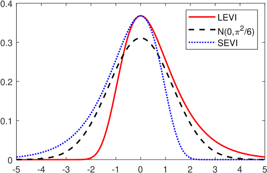
Figure 2: Probability density functions of the LEVI, NORM, and SEVI distributions

Figure 2 illustrates the pdfs of the LEVI and SEVI distributions. The LEVI distribution exhibits a strong right-skewness with a heavier upper tail in contrast to its lower tail, while SEVI exhibits the opposite (mirror image) behavior. As a symmetric benchmark, the normal pdf with the same variance is also plotted. The SEVI distribution is appropriate when there is a prior belief that the random utility component is more likely to have a negative rather than a positive or neutral effect on the total utility. Such a belief is plausible, and we have been unable to find a strong a priori argument against using a SEVI random component or a mixture of SEVI and LEVI components, as we discuss in Section 6.1.

This notion of random component skewness has to be seen as conditional on what alternative attributes and agent characteristics are observed by the econometrician. To see this, note that in the case of a linear latent utility model, $\varepsilon_{ij}$ consists of $(\tilde{X}_{ij}-E\tilde{X}_{ij})\tilde{\beta}_{0,x}$ for a scalar attribute $\tilde{X}_{ij}$ known to individual $i$ but not observable to the econometrician. If $\tilde{X}_{ij}$ has a negative skewness and $\tilde{\beta}_{0,x}>0$, then $(\tilde{X}_{ij}-E\tilde{X}_{ij})\tilde{\beta}_{0,x}$ will also have a negative skewness, implying that $\varepsilon_{ij}$ may exhibit left-skewness and follow the SEVI distribution. Thus, the inclusion or exclusion of a particular covariate may change the skewness of the stochastic utility component. More generally, the system utility may be misspecified, with the resulting specification error effectively becoming part of the stochastic utility. Given that specification errors can be manifest as left-skewed, symmetric, or right-skewed, the stochastic utility can display any of these forms of skewness as a consequence. This argument lends another support to the notion that the SEVI distribution of the stochastic utility is at least as plausible as the LEVI distribution.

A logical question at this point is whether the SEVI distribution belongs to the class of Generalized Extreme Value (GEV) distributions with the CDF given by $F_{\mathrm{GEV}}(a;\xi)=\exp(-\left(1+\xi a\right)^{-1/\xi})$ for some parameter $\xi.$ The SEVI distribution, however, does not align with a GEV distribution. Nor does it correspond to the marginal distribution of a multivariate extreme value (MEV) distribution with CDF:

$$F_{\mathrm{MEV}}(a_{1},\ldots,a_{J})=\exp(-\mathbb{G}\left(\exp\left(-a_{1}\right),\ldots,\exp\left(-a_{J}\right)\right),$$ (5)

for some function $\mathbb{G}$. In both cases, the marginal distribution is right-skewed instead of being left-skewed like a SEVI distribution. See, for example, Chapter 4 of Train, (2009). In principle, exploring an extension of the GEV or MEV family by using the SEVI as the marginal distribution, potentially encompassing the SEVI as a special case within this broader framework, could be considered for future research.

3.2 Choice Probabilities in the SEVI-based RUM

In a SEVI-based RUM, similar to a LEVI-based RUM, the choice probabilities also have closed-form expressions, albeit a bit more complex. To simplify the notation, we suppress the dependence of $V_{ij}\left(\beta_{0}\right)$ and $V_{i}\left(\beta_{0}\right):=(V_{i1}\left(\beta_{0}\right),\ldots,V_{iJ}\left(\beta_{0}\right))^{\prime}$ on $\beta_{0}$, and we write $U_{ij}:=U_{ij}\left(\beta_{0}\right),$ $V_{ij}:=V_{ij}\left(\beta_{0}\right),$ and $V_{i}:=V_{i}\left(\beta_{0}\right)$. We adopt the same convention for the realized values $v_{ij}\left(\beta_{0}\right)$ and $v_{i}\left(\beta_{0}\right)$ of $V_{ij}\left(\beta_{0}\right)$ and $V_{i}\left(\beta_{0}\right)$ in the theorem below.

Theorem 1

Assume that $U_{ij}=V_{ij}+\varepsilon_{ij}$, $j=1,2,\ldots,J$ where $\varepsilon_{i}:=\left(\varepsilon_{i1},\ldots,\varepsilon_{i,J}\right)^{\prime}$ is independent of $V_{i}$ and the elements of $\varepsilon_{i}$ follow independent and identical SEVI distributions. Then, under utility maximization, the probability of individual $i$ choosing alternative $j$ is

$$P^{\mathrm{SEVI}}\left(Y_{i}=j|v_{i}\right) :=P^{\mathrm{SEVI}}\left(Y_{i}=j|V_{i}=v_{i}\right)$$

$$=1+\sum_{\ell=1}^{J-1}\left(-1\right)^{\ell}\sum_{k_{1}<\ldots<k_{\ell}:\left\{k_{1},\ldots,k_{\ell}\right\}\subseteq\mathcal{J}_{-j}}\frac{\exp\left(-v_{ij}\right)}{\exp\left(-v_{ij}\right)+\sum_{k\in\left\{k_{1},\ldots,k_{\ell}\right\}}\exp\left(-v_{ik}\right)}$$ (6)

$$=1+\sum_{\ell=1}^{J-1}\left(-1\right)^{\ell}\sum_{k_{1}<\ldots<k_{\ell}:\left\{k_{1},\ldots,k_{\ell}\right\}\subseteq\mathcal{J}_{-j}}\frac{1}{1+\sum_{k\in\left\{k_{1},\ldots,k_{\ell}\right\}}\exp\left(-v_{ik}+v_{ij}\right)},$$

where, for $\mathcal{J}=\left\{1,\ldots,J\right\},$ $\mathcal{J}_{-j}=\mathcal{J}\backslash\left\{j\right\}$ is the subset of alternatives leaving the $j$-th alternative out.

Remark 1

In a standard LEVI conditional logit model, the choice probability is

$$P^{\mathrm{LEVI}}\left(Y_{i}=j|v_{i}\right)=\frac{\exp(v_{ij})}{\sum_{k=1}^{J}\exp\left(v_{ik}\right)}.$$ (7)

We can compare the choice probabilities across the SEVI and LEVI models using a few examples. When there are only two alternatives so that $J=2,$ we have, using Theorem 1,

$$P^{\mathrm{SEVI}}\left(Y_{i}=1|v_{i}\right) =1-\frac{\exp\left(-v_{i1}\right)}{\exp\left(-v_{i1}\right)+\exp\left(-v_{i2}\right)}$$

$$=\frac{\exp(-v_{i2})}{\exp(-v_{i1})+\exp(-v_{i2})}=\frac{\exp(v_{i1})}{\exp(v_{i1})+\exp(v_{i2})}.$$

The choice probability is exactly the same as what we obtain in a standard LEVI model. Therefore, in the presence of only two alternatives, it does not matter whether the stochastic utility follows the LEVI or SEVI distribution. This is because the difference between two independent LEVI or SEVI draws follows the same logistic distribution.

When there are more than two alternatives so that $J>2,$ the choice probabilities in a SEVI model are different from those in a LEVI model. Consider the case with $J=3.$ It follows from Theorem 1 that

$$P^{\mathrm{SEVI}}\left(Y_{i}=1|v_{i}\right) =1-\frac{\exp\left(-v_{i1}\right)}{\exp\left(-v_{i1}\right)+\exp\left(-v_{i2}\right)}-\frac{\exp\left(-v_{i1}\right)}{\exp\left(-v_{i1}\right)+\exp\left(-v_{i3}\right)}$$ (8)

$$+\frac{\exp\left(-v_{i1}\right)}{\exp\left(-v_{i1}\right)+\exp\left(-v_{i2}\right)+\exp\left(-v_{i3}\right)}.$$

This is clearly different from the LEVI choice probability, which is equal to

$$P^{\mathrm{LEVI}}\left(Y_{i}=1|v_{i}\right):=\frac{\exp\left(v_{i1}\right)}{\exp\left(v_{i1}\right)+\exp\left(v_{i2}\right)+\exp\left(v_{i3}\right)}.$$

To understand the formula for $P^{\mathrm{SEVI}}\left(Y_{i}=1|v_{i}\right),$ we can examine $1-P^{\mathrm{SEVI}}\left(Y_{i}=1|v_{i}\right),$ which represents the probability that alternative 1 is not chosen. The latter event can be expressed as a union of two events $\left\{U_{i1}\leq U_{i2}\right\}\cup\left\{U_{i1}\leq U_{i3}\right\}$, indicating that alternative 1 is dominated by either alternative 2 or alternative 3. But the probability of this union is

$$\Pr\left[\left\{U_{i1}\leq U_{i2}\right\}\cup\left\{U_{i1}\leq U_{i3}\right\}\right]$$

$$=\Pr\left[U_{i1}\leq U_{i2}\right]+\Pr\left[U_{i1}\leq U_{i3}\right]-\Pr\left[\left\{U_{i1}\leq U_{i2}\right\}\cap\left\{U_{i1}\leq U_{i3}\right\}\right]$$

$$=\Pr\left[-U_{i1}\geq-U_{i2}\right]+\Pr\left[-U_{i1}\geq-U_{i3}\right]-\Pr\left[\left\{-U_{i1}\geq-U_{i2}\right\}\cap\left\{-U_{i1}\geq-U_{i3}\right\}\right].$$

Each of the three probabilities above corresponds to a choice probability in a conventional LEVI model. Substituting the familiar LEVI formulas yields Equation (8), and Theorem 1 is a generalization of these arguments.

Remark 2

When $J=4,$ Theorem 1 reveals that

$$P^{\mathrm{SEVI}}\left(Y_{i}=1|v_{i}\right)$$

$$=1-\frac{\exp\left(-v_{i1}\right)}{\exp\left(-v_{i1}\right)+\exp\left(-v_{i2}\right)}-\frac{\exp\left(-v_{i1}\right)}{\exp\left(-v_{i1}\right)+\exp\left(-v_{i3}\right)}-\frac{\exp\left(-v_{i1}\right)}{\exp\left(-v_{i1}\right)+\exp\left(-v_{i4}\right)}$$

$$+\frac{\exp\left(-v_{i1}\right)}{\exp\left(-v_{i1}\right)+\exp\left(-v_{i2}\right)+\exp\left(-v_{i3}\right)}+\frac{\exp\left(-v_{i1}\right)}{\exp\left(-v_{i1}\right)+\exp\left(-v_{i2}\right)+\exp\left(-v_{i4}\right)}$$

$$+\frac{\exp\left(-v_{i1}\right)}{\exp\left(-v_{i1}\right)+\exp\left(-v_{i3}\right)+\exp\left(-v_{i4}\right)}$$

$$-\frac{\exp\left(-v_{i1}\right)}{\exp\left(-v_{i1}\right)+\exp\left(-v_{i2}\right)+\exp\left(-v_{i3}\right)+\exp\left(-v_{i4}\right)},$$

which involves enumerating all choice subsets that contain the first alternative. In contrast, the corresponding choice probability in a LEVI model is

$$P^{\mathrm{LEVI}}\left(Y_{i}=1|v_{i}\right)=\frac{\exp\left(v_{i1}\right)}{\left[\exp\left(v_{i1}\right)+\exp\left(v_{i2}\right)+\exp\left(v_{i3}\right)+\exp\left(v_{i4}\right)\right]},$$

which involves only the largest choice set. As shown in Figure 1, and later, when $J$ becomes larger than 2, the choice probabilities in a SEVI model can be different from those in a LEVI model in an economically meaningful way. This has practical implications, underscoring the need for careful consideration when formulating distribution assumptions in discrete choice modeling.

Remark 3

When $v_{ij}=v_{ik}$ for all $j$ and $k,$ we have

$$P^{\mathrm{SEVI}}\left(Y_{i}=j|v_{i}\right) =1+\sum_{\ell=1}^{J-1}\left(-1\right)^{\ell}\sum_{k_{1}<\ldots<k_{\ell}:\left\{k_{1},\ldots,k_{\ell}\right\}\subseteq\mathcal{J}_{-j}}\frac{1}{\ell+1}$$

$$=\sum_{\ell=0}^{J-1}\left(-1\right)^{\ell}\binom{J-1}{\ell}\frac{1}{\ell+1}=\int_{0}^{1}\sum_{\ell=0}^{J-1}\left(-1\right)^{\ell}\binom{J-1}{\ell}s^{\ell}ds$$

$$=\int_{0}^{1}\left(1-s\right)^{J-1}ds=\frac{1}{J}.$$

This result can also be obtained by using a symmetric argument. Since all alternatives have the same systematic utility, they are indistinguishable and hence have an equal chance of being chosen. The result is the same as that obtained under the LEVI assumption. On the other hand, when $v_{ij}$ increases and dominates all other $v_{ik}$ for $k\neq j,$ $P^{\mathrm{SEVI}}\left(Y_{i}=j|v_{i}\right)$ approaches 1. The choice probability $P^{\mathrm{SEVI}}\left(Y_{i}=j|v_{i}\right)$ can, therefore, be regarded as a type of softmax function that maps $\mathbb{R}^{J}$ into $\left(0,1\right)^{J}.$ For example, it maps $\left(1,2,8\right)$ into $(4.24\times 10^{-4},$ $2.29\times 10^{-3},0.997),$ which amounts to assigning almost all probability mass to the element with maximal systematic utility. This result is qualitatively similar to that obtained under the LEVI assumption.

Remark 4

The probability of choosing alternative $j$ in a SEVI model involves a summation over all subsets of $\mathcal{J}_{-j},$ resulting in an iteration over a total of $2^{J-1}$ subsets of alternatives. The choice probability in a LEVI model takes a simpler, more convenient form. While the choice probability in a SEVI model is considerably richer than that in a LEVI model, the SEVI model has a computational disadvantage when $J$ is large. To mitigate this, we employ Gosper’s hack, a technique rooted in bitwise operations, to streamline the iteration process efficiently. Additionally, by leveraging the arguments following Proposition 4.4 in Ross, (2013), it can be shown that for any $M<J$:

$$\left|P^{\mathrm{SEVI}}\left(Y_{i}=j|v_{i}\right)-P_{M}^{\mathrm{SEVI}}\left(Y_{i}=j|v_{i}\right)\right|\leq\sum_{k_{1}<\ldots<k_{M}:\left\{k_{1},\ldots,k_{M}\right\}\subseteq\mathcal{J}_{-j}}\frac{1}{1+\sum_{k\in\left\{k_{1},\ldots,k_{\ell}\right\}}\exp\left(-v_{ik}+v_{ij}\right)}$$ (9)

where

$$P_{M}^{\mathrm{SEVI}}\left(Y_{i}=j|v_{i}\right)=1+\sum_{\ell=1}^{M-1}\left(-1\right)^{\ell}\sum_{k_{1}<\ldots<k_{\ell}:\left\{k_{1},\ldots,k_{\ell}\right\}\subseteq\mathcal{J}_{-j}}\frac{1}{1+\sum_{k\in\left\{k_{1},\ldots,k_{\ell}\right\}}\exp\left(-v_{ik}+v_{ij}\right)}.$$

This allows us to approximate $P^{\mathrm{SEVI}}\left(Y_{i}=j|v_{i}\right)$ by $P_{M}^{\mathrm{SEVI}}\left(Y_{i}=j|v_{i}\right)$ with a well-controlled approximation error. Note that $P_{M}^{\mathrm{SEVI}}\left(Y_{i}=j|v_{i}\right)$ takes the same form as $P^{\mathrm{SEVI}}\left(Y_{i}=j|v_{i}\right)$ but involves subsets of at most $M-1$ alternatives, and so it is computationally less intensive when $M$ is smaller than $J.$ To achieve a desired level of precision, we can choose $M$ large enough and stop iterating over subsets of more than $M-1$ alternatives. Combining Gosper’s hack with an early stopping makes it computationally easy to estimate a SEVI model for $J$ as large as 14. Section 5.3 reports and compares the computation times for various models using simulated data with typical sample size and attribute numbers. Section 7 contains a comparison of computation times for real data applications.

Remark 5

For the SEVI model with a linear parametrization of $V_{ij}\left(\beta_{0}\right),$ if $Z_{i}$ is not present so that $V_{ij}\left(\beta_{0}\right)=X_{ij}\beta_{0,x},$ then the model is called a conditional SEVI (logit) model. As an extension of the basic model, we can allow the coefficient on $X_{ij}$ to be alternative specific and so we may have $V_{ij}\left(\beta_{0}\right)=X_{ij}\beta_{0,x,j}.$ On the other hand, if $X_{ij}$ is not present so that $V_{ij}\left(\beta_{0}\right)=Z_{i}\beta_{0,z,j},$ then the model is called a multinomial SEVI (logit) model. These forms can be combined so that $V_{ij}\left(\beta_{0}\right)=\alpha_{j}+Z_{i}\beta_{0,z,j}+X_{ij}\beta_{0,x}+W_{ij}\beta_{0,w,j},$ which provides the same flexibility as in a standard LEVI (logit) model. As in a standard multinomial LEVI (logit) model, not all of $\beta_{0,z,j}$’s are identified, and we need to normalize one of them, say $\beta_{0,z,J},$ to be zero.

To illustrate the difference between the SEVI and LEVI models, we simulate the choice probabilities when $V_{ij}\left(\beta_{0}\right)=X_{ij}\beta_{0,x}$ (there is no individual-specific characteristic or alternative-specific constant), and the stochastic utility is iid SEVI or LEVI. We set the number of covariates $L$ in $X_{ij}$ to be $3$ (there are three attributes for each alternative) and let $\beta_{0}=\beta_{0,x}=(1,2,1)^{\prime}.$ We consider two data generating processes (DGP) for the attributes $\left\{X_{ij}\right\}$. In the first DGP, for each $i$ and $j,$ we let $X_{ij,\ell}$ be iid $N(0,\pi^{2}\omega_{j}^{2}/36)$ over $\ell=1,2,3$ where

$$\omega_{j}=\frac{j-\left(J+1\right)/2}{\sqrt{\left(J^{2}-1\right)/12}},\text{ }j=1,\ldots,J.\text{ }$$ (10)

Here, $\left(\omega_{1},\ldots,\omega_{J}\right)$ is a just standardized version of the sequence ($1,2,\ldots,J$). In this case, each attribute $X_{ij,\ell}$ becomes more dispersed when the alternative label $j$ is closer to $1$ or $J$. As a result, the mean choice probabilities (i.e., $E\Pr\left(Y_{i}=j|V_{i}\right)$) are not all the same across the alternatives. In the second DGP, for each $i$ and $j,$ we let $X_{ij,\ell}$ be iid $N(0,\pi^{2}/36)$ over $\ell=1,2,3.$ In this case, the attributes have the same distribution across the alternatives, and the mean choice probabilities are the same across all alternatives. Under these two DGPs for $\left\{X_{ij}\right\},$ the variances of the systematic utility $V_{ij}\left(\beta_{0}\right)=X_{ij}\beta_{0}$ are $\pi^{2}\omega_{j}^{2}/6$ and $\pi^{2}/6,$ respectively. These variances are comparable to $\pi^{2}/6,$ the variance of the stochastic utility.

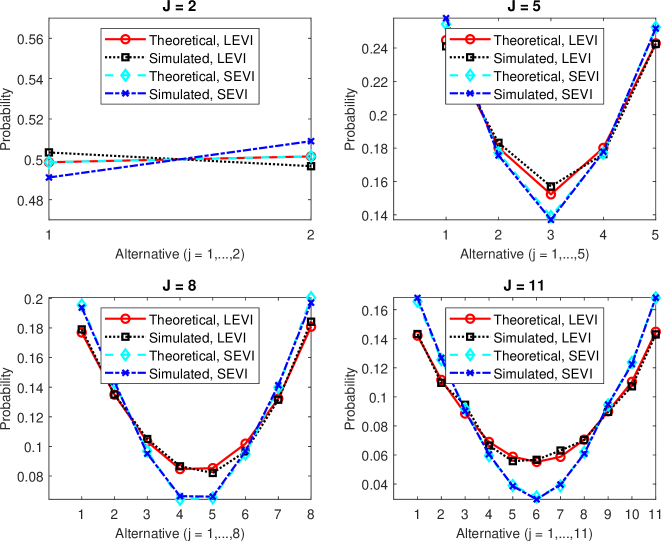
Figure 3: Simulated choice probabilities and the average of theoretical choice probabilities against alternative labels $(j=1,\ldots,J)$ for a sample of $n=10,000$ individuals when $X_{ij,\ell}$ is iid $N(0,\pi^{2}\omega_{j}^{2}/36)$

For each model, we compute the choice probabilities according to the theoretical formulae (i.e., (6) under the SEVI and (7) under the LEVI), and take the average of these choice probabilities over 10,000 individuals. We also simulate the decisions of 10,000 independent individuals and compute the proportion of individuals choosing each alternative. Figure 3 reports results for various $J$ values when $X_{ij,\ell}$ $\thicksim$ iid $N(0,\pi^{2}\omega_{j}^{2}/36).$ Not surprisingly, since the sample size is large, the average theoretical choice probabilities match the simulated choice proportions well for both the SEVI and LEVI models. When $J=2,$ the theoretical choice probabilities are the same across the two models. With only two alternatives, the simulated choice shares are very close across the two models, but not identical due to simulation errors. When $J>2,$ for alternatives with relatively higher choice probabilities under the LEVI, the SEVI model assigns a higher choice probability than the LEVI model. On the other hand, when $J>2,$ for alternatives with a relatively lower choice probability under the LEVI, the SEVI model assigns a lower choice probability than the LEVI model. The difference between the choice probabilities across the two models grows with $J.$ The choice probability in a SEVI model is closer to the “arg max” function than that in a LEVI model. In this context, a SEVI model leans more towards embodying the concept of “the winner takes it all” than a LEVI model. More specifically, given the same set of systematic utilities, the probability of choosing the alternative with the maximum systematic utility in a SEVI model tends to be larger than that in a LEVI model.

Next, we report the results when $X_{ij,\ell}$ is iid $N(0,\pi^{2}/36)$, but we use a different type of plot. Figure 4 provides a scatter plot of the ratio of the choice probabilities in the SEVI and LEVI models (i.e., $P^{\mathrm{SEVI}}/P^{\mathrm{LEVI}})$ against $P^{\mathrm{LEVI}}$. Instead of examining the average choice probabilities as done in Figure 3, we consider the choice probability of choosing a specific alternative (here, we use alternative 1 without loss of generality) for each realization of the systematic utilities. Figure 5 provides a supplementary illustration, offering a closer examination of certain details.

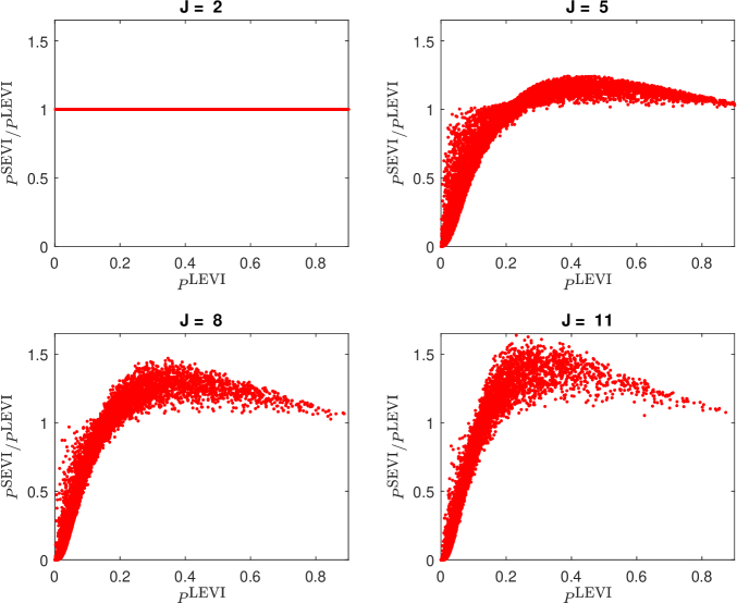
Figure 4: Scatter plot of the ratio of choice probabilities in the SEVI and LEVI models ($P^{\mathrm{SEVI}}/P^{\mathrm{LEVI}})$ against the choice probability in the LEVI model ($P^{\mathrm{LEVI}})$ with identical systematic utilities when $X_{ij,\ell}$ is iid $N(0,\pi^{2}/36)$

In both Figure 4 and Figure 5, the systematic utilities are held constant for each data point with either LEVI errors or SEVI errors. We note from these two figures that when $J>2$ and $P^{\mathrm{LEVI}}$ is low, $P^{\mathrm{SEVI}}$ can be more than 50 percent lower. For example, when there are five alternatives ($J=5$) and $P^{\mathrm{LEVI}}=0.1,$ $P^{\mathrm{SEVI}}$ can be as low as $0.05$. The LEVI probability can be roughly twice as large as the SEVI probability. Thus, from a practical point of view, a choice between the two models can have an enormous impact on predicting a lift for a minor brand with a market share between 5% and 10%. On the other hand, when $J>2$ and $P^{\mathrm{LEVI}}$ is high, $P^{\mathrm{SEVI}}$ tends to be higher. For example, when $J=5$ and $P^{\mathrm{LEVI}}=0.4,$ $P^{\mathrm{SEVI}}$ can be 20 percent higher; when $J=11$ and $P^{\mathrm{LEVI}}=0.3,$ $P^{\mathrm{SEVI}}$ can be 50 percent higher. The patterns we observe here are similar to those in Figure 1. The difference in the choice probabilities across the two models can be important in various contexts, ranging from antitrust actions to production planning.

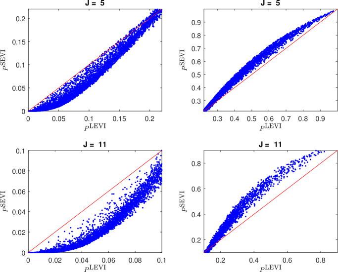
Figure 5: Scatter plot of the choice probability in the SEVI model versus that in the LEVI model with left and right panels having different ranges for the horizontal axis ($X_{ij,\ell}$ is iid $N(0,\pi^{2}/36))$

Figure 5 shows that when $J=5$ and the LEVI probability is below 0.20, the corresponding SEVI probability is lower. When the LEVI probability is above 0.20, the corresponding SEVI probability is higher. Similar patterns are found for other values of $J.$ These qualitative patterns are consistent with what we find in Figure 3. The vector of choice probabilities in the SEVI model (i.e., $[P^{\mathrm{SEVI}}(Y=1),\ldots,P^{\mathrm{SEVI}}\left(Y=J\right)]$) is closer to the vertices of the probability simplex than that in the LEVI model. In other words, $[P^{\mathrm{SEVI}}(Y=1),\ldots,P^{\mathrm{SEVI}}\left(Y=J\right)]$ is closer to $\arg\max\left(v_{1},\ldots,v_{J}\right):=(0,\ldots,1,\ldots,0),$ a $0$-$1$ vector with the $j$-th element equal to 1 if and only if $v_{j}$ is the maximum value of $\left(v_{1},\ldots,v_{J}\right).$

We now offer insights into why the probability vector $[P^{\mathrm{SEVI}}(Y=1),\ldots,P^{\mathrm{SEVI}}\left(Y=J\right)]$ is closer to the one-hot encoding of $\arg\max\left(v_{1},\ldots,v_{J}\right)$ than $[P^{\mathrm{LEVI}}(Y=1),\ldots,P^{\mathrm{LEVI}}\left(Y=J\right)].$ When $J\geq 3,$ the top two values among $J$ independent draws from the stochastic utility distribution are more likely to be above or equal to the median of this distribution rather than below it. For a draw from the LEVI distribution, conditional on being above the median, the mean is 1.545 and the standard deviation is 1.079. In contrast, for the SEVI case, these values are 0.391 and 0.500, respectively. Hence, the absolute difference between any two above-the-median draws from the LEVI distribution is expected to be larger than that for the SEVI distribution. In fact, Monte Carlo simulations show that the former first-order stochastically dominates the latter (see Figure S.1). This implies that two above-the-median draws from the SEVI distribution are more likely to be closer to each other than those from the LEVI distribution. Therefore, with more than two alternatives, it is less probable for the stochastic utility components under the SEVI to make a difference in determining which alternative has the highest total utility. As a result, in the presence of more than two alternatives, the choice probabilities under the SEVI are better aligned with the systematic utilities than those under the LEVI. In other words, in a SEVI model with $J\geq 3$, the observed choice is more likely to correspond to the choice that maximizes the systematic utility than in a LEVI model. See Figure S.2 for an additional illustration.

3.3 Algebraic Relation between SEVI and LEVI Choice Probabilities

To relate the choice probabilities under SEVI and LEVI assumptions, we consider a general latent utility model $U_{ij}=V_{ij}+\varepsilon_{ij},$ $j=1,\ldots,J$ where $\varepsilon_{ij}$ is iid across $j=1,\ldots,J$ and may follow either SEVI or LEVI, $\varepsilon_{i}=\left(\varepsilon_{i1},\ldots,\varepsilon_{iJ}\right)$ is independent of $V_{i}=(V_{i1},\ldots,V_{iJ})$. For any alternative $j$ and any subset of alternatives $\mathcal{S}_{\ell}$ that does not include alternative $j,$ we let

$$P^{\mathrm{SEVI}}(Y_{i} =j|\mathcal{S}_{\ell}\cup j,V_{i}=v_{i})=\Pr(Y_{i}=j|\mathcal{S}_{\ell}\cup j,V_{i}=v_{i},\varepsilon_{im}\thicksim iid\text{ }\mathrm{SEVI}\text{ over }m\in\mathcal{J}),$$

$$P^{\mathrm{LEVI}}(Y_{i} =j|\mathcal{S}_{\ell}\cup j,V_{i}=v_{i})=\Pr(Y_{i}=j|\mathcal{S}_{\ell}\cup j,V_{i}=v_{i},\varepsilon_{im}\thicksim iid\text{ }\mathrm{LEVI}\text{ over }m\in\mathcal{J}),$$

which are the probabilities of individual $i$ choosing alternative $j$ from the subset $\mathcal{S}_{\ell}\cup j:=$ $\mathcal{S}_{\ell}\cup\left\{j\right\}$ under SEVI and LEVI errors, respectively. It is important to point out that in the above definition, the probabilities depend on the choice subset under consideration.

Proposition 2

The choice probabilities under the SEVI and LEVI satisfy the following relations:

$$P^{\mathrm{SEVI}}(Y_{i} =j|\mathcal{J},V_{i}=v_{i})$$

$$=1+\sum_{\ell=1}^{J-1}\left(-1\right)^{\ell}\sum_{k_{1}<\ldots<k_{\ell}:\text{ }\mathcal{S}_{\ell}=\left\{k_{1},\ldots,k_{\ell}\right\}\subseteq\mathcal{J}_{-j}}P^{\mathrm{LEVI}}\left(Y_{i}=j|\mathcal{S}_{\ell}\cup j,V_{i}=-v_{i}\right);$$

$$P^{\mathrm{LEVI}}(Y_{i} =j|\mathcal{J},V_{i}=v_{i})$$

$$=1+\sum_{\ell=1}^{J-1}\left(-1\right)^{\ell}\sum_{k_{1}<\ldots<k_{\ell}:\text{ }\mathcal{S}_{\ell}=\left\{k_{1},\ldots,k_{\ell}\right\}\subseteq\mathcal{J}_{-j}}P^{\mathrm{SEVI}}\left(Y_{i}=j|\mathcal{S}_{\ell}\cup j,V_{i}=-v_{i}\right).$$

The proposition shows an intrinsic connection between the choice probabilities under the two assumptions of the stochastic utility. Note that the right-hand side of each relation involves the probabilities of choosing alternative $j$ over all subsets of alternatives that contain alternative $j$ but under a “reflected” model for $V_{i}$ ($V_{i}=v_{i}$ on the left-hand side becomes $V_{i}=-v_{i}$ on the right-hand side).

By taking the difference between the two equations in Proposition 2, we have

$$P^{\mathrm{SEVI}}(Y_{i} =j|\mathcal{J},V_{i}=v_{i})-P^{\mathrm{LEVI}}(Y_{i}=j|\mathcal{J},V_{i}=v_{i})$$

$$=\sum_{\ell=2}^{J-1}\left(-1\right)^{\ell-1}\sum_{k_{1}<\ldots<k_{\ell}:\text{ }\mathcal{S}_{\ell}=\left\{k_{1},\ldots,k_{\ell}\right\}\subseteq\mathcal{J}_{-j}}\left[P^{\Delta}\left(Y_{i}=j|\mathcal{S}_{\ell}\cup j,V_{i}=-v_{i}\right)\right],$$

where

$$P^{\Delta}\left(Y_{i}=j|\mathcal{S}_{\ell}\cup j,V_{i}=-v_{i}\right)=P^{\mathrm{SEVI}}\left(Y_{i}=j|\mathcal{S}_{\ell}\cup j,V_{i}=-v_{i}\right)-P^{\mathrm{LEVI}}\left(Y_{i}=j|\mathcal{S}_{\ell}\cup j,V_{i}=-v_{i}\right).$$

So, the difference in the SEVI and LEVI probabilities of choosing alternative $j$ from the entire choice set $\mathcal{J}$ is an aggregation of the probability differences from choosing alternative $j$ from all subsets of alternatives that contain $j$ but with flipped systematic utilities. This is a recursive relationship, as each probability difference on the right-hand side can be represented in the same fashion as the left-hand side. An intriguing question emerges: can the difference in choice probabilities be fully captured by a simple index that measures the concentration of the systematic utilities? Given the intricate recursive relationship described above and the highly nonlinear dependence of the probability difference on systematic utilities, as shown in Figure S.3, it appears unlikely that commonly used measures like the Gini coefficient or the Herfindahl-Hirschman index would be sufficient for this task. However, in empirical practice, particularly for moderately sized $J$, these measures are likely to prove useful in predicting differences in choice probabilities.

The second relation in Proposition 2 can be presented equivalently as follows:

$$P^{\mathrm{LEVI}}(Y_{i} =j|\mathcal{J},V_{i}=-v_{i})$$

$$=1+\sum_{\ell=1}^{J-1}\left(-1\right)^{\ell}\sum_{k_{1}<\ldots<k_{\ell}:\mathcal{S}_{\ell}:=\left\{k_{1},\ldots,k_{\ell}\right\}\subseteq\mathcal{J}_{-j}}P^{\mathrm{SEVI}}\left(Y_{i}=j|\mathcal{S}_{\ell}\cup j,V_{i}=v_{i}\right).$$ (11)

Since $P^{\mathrm{LEVI}}(Y_{i}=j|\mathcal{J},V_{i}=-v_{i})$ is nonnegative, the sum in (11) is also nonnegative. This sum is a special Block-Marschak polynomial (Block and Marschak, (1960)). In the presence of a finite number of alternatives, it is well-known in the stochastic choice theory that the nonnegativity of Block-Marschak polynomials is both necessary and sufficient for a random choice rule to have an additive random utility representation. For a detailed discussion, see, for example, Chapters 1 and 2 of the recent book by Strzalecki, (2023). In the present setting, the choice probabilities under SEVI are derived from random utility maximization and as such, they trivially have an additive random utility representation. The significance of (11) is that it provides a simple characterization of a special Block-Marschak polynomial.

More generally, let $j$ be a target alternative of interest and

$$\mathcal{D}_{j}:=\left\{\left(d_{1},\ldots,d_{\rho},j\right):d_{1}<\ldots<d_{\rho}\text{ and }\left(d_{1}<\ldots<d_{\rho}\right)\subseteq\mathcal{J}_{-j}\right\}$$

be a subset of alternatives that includes alternative $j.$ Then, the (general) Block-Marschak polynomial for our probability choice rule under SEVI errors is defined to be

$$\mathcal{K}^{\mathrm{SEVI}}(j,\mathcal{D}_{j})$$

$$:=\Pr\left(Y_{i}=j|\mathcal{D}_{j},V_{i}=v_{i},\varepsilon_{im}\thicksim iid\text{ }\mathrm{SEVI}\text{ over }m\in\mathcal{J}\right)$$

$$+\sum_{\ell=1}^{J-\left|\mathcal{D}_{j}\right|}\left(-1\right)^{\ell}\sum_{k_{1}<\ldots<k_{\ell}:\mathcal{S}_{\ell}:=\left\{k_{1},\ldots,k_{\ell}\right\}\subseteq\mathcal{J}\backslash\mathcal{D}_{j}}P^{\mathrm{SEVI}}\left(Y_{i}=j|\mathcal{S}_{\ell}\cup\mathcal{D}_{j},V_{i}=v_{i}\right).$$

Note that when $\mathcal{D}_{j}=\left\{j\right\},$ the first term in $\mathcal{K}^{\mathrm{SEVI}}(j,\mathcal{D}_{j})$ becomes $1$ and $\mathcal{K}^{\mathrm{SEVI}}(j,\mathcal{D}_{j})$ reduces to the special Block-Marschak polynomial in (11). We can show that $\mathcal{K}^{\mathrm{SEVI}}(j,\mathcal{D}_{j})$ is the probability that the $j$-th alternative dominates all other alternatives in $\mathcal{D}_{j}$ but is dominated by the alternatives that are not in $\mathcal{D}_{j}.$ See, for example, Barberá and Pattanaik, (1986). Hence, $\mathcal{K}^{\mathrm{SEVI}}(j,\mathcal{D}_{j})\geq 0$ for all $\left(j,\mathcal{D}_{j}\right),$ which is consistent with the nonnegativity of Block-Marschak polynomials for any additive RUM model.

The Block-Marschak polynomial $\mathcal{K}^{\mathrm{SEVI}}(j,\mathcal{D}_{j})$ is precisely the probability relevant for rank-ordered data. While using the SEVI model for rank-ordered data necessitates additional research, the formula for $\mathcal{K}^{\mathrm{SEVI}}(j,\mathcal{D}_{j})$ provides a good starting point.

3.4 Patterns of Substitution and the Lack of IIA

In this subsection, we compute $\partial P^{\mathrm{SEVI}}\left(Y_{i}=k|v_{i}\right)/\partial v_{ij}$, the effect of an infinitesimal change in alternative $j$’s systematic utility (as perceived by individual $i$) on the probability of individual $i$ choosing alternative $k.$ This computation is essential for determining $\partial P^{\mathrm{SEVI}}\left(Y_{i}=k|v_{i}\right)/\partial X_{ij},$ the effect of changing alternative $j$’s attributes on the probability of choosing alternative $k.$

For notational economy, we let $P_{ik}^{\mathrm{SEVI}}:=P^{\mathrm{SEVI}}\left(Y_{i}=k|v_{i}\right).$ We have, using Proposition 2 and some simple calculations,

$$\frac{\partial P_{ij}^{\mathrm{SEVI}}}{\partial v_{ij}}=-\sum_{\ell=1}^{J-1}\left(-1\right)^{\ell}\sum_{k_{1}<\ldots<k_{\ell}:\mathcal{S}_{\ell}=\left\{k_{1},\ldots,k_{\ell}\right\}\subseteq\mathcal{J}_{-j}}P^{\mathrm{LEVI}}(Y_{i}=j|\mathcal{S}_{\ell}\cup j,-v_{i})P^{\mathrm{LEVI}}(Y_{i}\neq j|\mathcal{S}_{\ell}\cup j,-v_{i}),$$ (12)

where for $\mathcal{S}_{\ell-1}=\left\{k_{1},\ldots,k_{\ell-1}\right\}\subseteq\mathcal{J}_{-j},$

$$P^{\mathrm{LEVI}}(Y_{i} =j|\mathcal{S}_{\ell}\cup j,-v_{i})=\frac{\exp(-v_{ij})}{\sum_{m\in\mathcal{S}_{\ell}\cup j}\exp\left(-v_{im}\right)},$$

$$P^{\mathrm{LEVI}}(Y_{i} \neq j|\mathcal{S}_{\ell}\cup j,-v_{i})=1-P^{\mathrm{LEVI}}(Y_{i}=j|\mathcal{S}_{\ell}\cup j,-v_{i}).$$

Furthermore, for $k\neq j,$

$$\frac{\partial P_{ij}^{\mathrm{SEVI}}}{\partial v_{ik}} =\sum_{\ell=1}^{J-1}\left(-1\right)^{\ell}\sum_{k_{1}<\ldots<k_{\ell-1}:\mathcal{S}_{\ell-1}=\left\{k_{1},\ldots,k_{\ell-1}\right\}\subseteq\mathcal{J}_{-\left(j,k\right)}}$$

$$P^{\mathrm{LEVI}}(Y_{i}\overset{}{=}j|\mathcal{S}_{\ell-1}\cup\left\{j,k\right\},-v_{i})\cdot P^{\mathrm{LEVI}}(Y_{i}\overset{}{=}k|\mathcal{S}_{\ell-1}\cup\left\{j,k\right\},-v_{i}),$$ (13)

where for $\mathcal{S}_{\ell-1}=\left\{k_{1},\ldots,k_{\ell-1}\right\}\subseteq\mathcal{J}_{-\left(j,k\right)},$ a subset of $\mathcal{J}$ excluding $j$ and $k,$

$$P^{\mathrm{LEVI}}(Y_{i} =j|\mathcal{S}_{\ell}\cup\left\{j,k\right\},-v_{i})=\frac{\exp(-v_{ij})}{\sum_{m\in\mathcal{S}_{\ell}\cup\left\{j,k\right\}}\exp\left(-v_{im}\right)},$$

$$P^{\mathrm{LEVI}}(Y_{i} =k|\mathcal{S}_{\ell}\cup\left\{j,k\right\},-v_{i})=\frac{\exp(-v_{ik})}{\sum_{m\in\mathcal{S}_{\ell}\cup\left\{j,k\right\}}\exp\left(-v_{im}\right)}.$$

In equation (13), the first term in the summation (i.e., when $\ell=1)$ is understood to be

$$-\frac{\exp(-v_{ij})}{\left[\exp(-v_{ij})+\exp\left(-v_{ik}\right)\right]}\frac{\exp(-v_{ik})}{\left[\exp(-v_{ij})+\exp\left(-v_{ik}\right)\right]}.$$

Equation (13) reveals that

$$\frac{\partial P_{ij}^{\mathrm{SEVI}}}{\partial v_{ik}}=\frac{\partial P_{ik}^{\mathrm{SEVI}}}{\partial v_{ij}}$$ (14)

for any $k$ and $j.$ That is, the choice probabilities satisfy a symmetry property analogous to Slutsky symmetry in continuous choice models.

The expression of $\partial P_{ij}^{\mathrm{SEVI}}/\partial v_{ik}$ can be used to derive the score function, which is essential for finding the MLE and developing the asymptotic theory. It can also be employed to examine whether the IIA property holds in a SEVI model when $J\geq 3$. For the IIA to hold, the cross (semi)elasticity $\partial\log P_{ij}^{\mathrm{SEVI}}/\partial v_{ik}$ should be the same for all $j\neq k.$ That is,

$$\frac{\partial\log P_{ij_{1}}^{\mathrm{SEVI}}}{\partial v_{ik}}=\frac{\partial\log P_{ij_{2}}^{\mathrm{SEVI}}}{\partial v_{ik}}$$

for all $j_{1}\neq j_{2}\neq k.$ However, this condition is not met, as is clear from (13). Alternatively, for the IIA to hold, the probability ratio $P_{ij_{1}}^{\mathrm{SEVI}}/P_{ij_{2}}^{\mathrm{SEVI}}$ should not depend on the systematic utilities of alternatives other than alternatives $j_{1}$ and $j_{2}.$ However, it is evident that the probability ratio does depend on the systematic utilities of all alternatives, indicating that the IIA does not hold.

To illustrate the violation of the IIA in a SEVI model with $J\geq 3$, we start with a scenario featuring two initial alternatives: individuals must choose between alternative 1 and alternative 2. In this context, the choice between the SEVI or LEVI does not matter. For a fixed scale value $s_{1}$ (we set $v_{1}$ to $\log 1$ so that $s_{1}=\exp(v_{1})=1$), we examine a range of possible values for $s_{2}:=\exp\left(v_{2}\right)\in\left\{0.01:0.01:3\right\},$ a grid of values from 0.01 to 3 with increment 0.01. Each combination of $\left(s_{1},s_{2}\right)$ corresponds to a probability ratio:

$$\frac{P(Y=2|v_{1},v_{2})}{P(Y=1|v_{1},v_{2})}=\frac{P^{\mathrm{SEVI}}(Y=2|v_{1},v_{2})}{P^{\mathrm{SEVI}}(Y=1|v_{1},v_{2})}=\frac{P^{\mathrm{LEVI}}(Y=2|v_{1},v_{2})}{P^{\mathrm{LEVI}}(Y=1|v_{1},v_{2})}=\frac{\exp(v_{2})}{\exp(v_{1})}=s_{2}.$$

Next, we introduce a third alternative with its scale value $s_{3}=\exp\left(v_{3}\right)\in\left\{0.01:0.01:3\right\}$, the same grid for $s_{2}.$ We investigate how the probability ratio of choosing alternative 2 versus alternative 1 changes. This ratio now depends on whether the stochastic utilities follow the SEVI or LEVI distribution.

The difference of the ratios under SEVI and LEVI models, denoted as $D_{\mathrm{PR}},$ is

$$D_{\mathrm{PR}} =\frac{P^{\mathrm{SEVI}}(Y=2|v_{1},v_{2},v_{3})}{P^{\mathrm{SEVI}}(Y=1|v_{1},v_{2},v_{3})}-\frac{P^{\mathrm{LEVI}}(Y=2|v_{1},v_{2},v_{3})}{P^{\mathrm{LEVI}}(Y=1|v_{1},v_{2},v_{3})}$$

$$=\frac{P^{\mathrm{SEVI}}(Y=2|v_{1},v_{2},v_{3})}{P^{\mathrm{SEVI}}(Y=1|v_{1},v_{2},v_{3})}-\frac{P^{\mathrm{LEVI}}(Y=2|v_{1},v_{2})}{P^{\mathrm{LEVI}}(Y=1|v_{1},v_{2})}$$

$$=\frac{P^{\mathrm{SEVI}}(Y=2|v_{1},v_{2},v_{3})}{P^{\mathrm{SEVI}}(Y=1|v_{1},v_{2},v_{3})}-\frac{P^{\mathrm{SEVI}}(Y=2|v_{1},v_{2})}{P^{\mathrm{SEVI}}(Y=1|v_{1},v_{2})}$$

$$=\frac{P^{\mathrm{SEVI}}(Y=2|v_{1},v_{2},v_{3})}{P^{\mathrm{SEVI}}(Y=1|v_{1},v_{2},v_{3})}-s_{2}.$$

Here we have used properties of the LEVI probabilities. By the third equality above, $D_{\mathrm{PR}}$ also gauges the extent of IIA violation. With $s_{1}$ set to 1, $D_{\mathrm{PR}}$ is a function of $s_{2}$ and $s_{3}$, so we can write it as $D_{\mathrm{PR}}(s_{2},s_{3}).$ We present a contour plot of this function in Figure 6. To aid interpretation, we label the horizontal axis as $P(Y=2|v_{1},v_{2})/P(Y=1|v_{1},v_{2})=\exp(v_{2})=s_{2},$ representing the initial probability ratio with only two alternatives available.

It is clear from Figure 6 that $D_{\mathrm{PR}}(s_{2},s_{3})$ is not a zero function. After the introduction of the third alternative, the market shares of alternatives 1 and 2 do not decrease proportionally in the SEVI model as what happens in the LEVI model, indicating a violation of the IIA.

Figure 6 also shows that there are two scenarios where $D_{\mathrm{PR}}(s_{2},s_{3})$ equals zero or becomes approximately zero. First, $D_{\mathrm{PR}}(s_{2},s_{3})$ equals zero when alternatives 1 and 2 have the same initial market share (i.e., $P(Y=2|v_{1},v_{2})/P(Y=1|v_{1},v_{2})=s_{2}=1)$. This is expected, as in this case, the first two alternatives are indistinguishable, and their market shares reduce proportionally in both the LEVI and SEVI models when the third alternative is introduced. Second, $D_{\mathrm{PR}}(s_{2},s_{3})$ approaches zero when one of the alternatives becomes almost completely dominant in the market. This corresponds to a scenario where either $s_{2}$ is small and $s_{3}$ is very large, or $s_{3}$ is small and $s_{2}$ is very large. Hence, the difference between a SEVI model and a LEVI model may not be large when there is clearly a dominant player in the market who commands almost the entire market, and their disparities become more apparent when no alternative has nearly all market share.

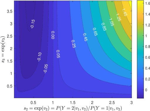
Figure 6: Contour plot of the difference of the choice probability ratios $D_{\mathrm{PR}}(s_{2},s_{3})$ between the SEVI and LEVI models against $\left[s_{2},s_{3}\right]$ when $s_{1}=1$

In an additively separable RUM with $U_{ij}=V_{ij}+\varepsilon_{ij},$ as considered here, it is well known that the IIA property holds for any $J\geq 3$ if and only if the stochastic utility $\varepsilon_{ij}$ follows the LEVI distribution (cf., Yellott, (1977)). Under certain conditions that permit an infinite $J,$ it can be shown that in a random utility model with possibly nonseparable utility functions, the IIA holds for any $J\geq 3$ only if the latent utility $U_{ij}$ can be represented as $H\left(V_{ij}+\varepsilon_{ij}\right)$ for some strictly increasing function $H\left(\cdot\right)$ and LEVI-distributed $\varepsilon_{ij}.$ This result is a corollary to Theorem 1 of Dagsvik, (2016); see also Lindberg and Smith, (2017) and the references therein. The SEVI model does not have the required representation, and this provides another perspective on the absence of the IIA property in the SEVI model when $J\geq 3.$

One consequence of the lack of IIA is that we cannot consistently estimate the preference parameters in a SEVI model using the random sampling approach. In this approach, for each decision maker, we sample a random subset of alternatives that contains the chosen alternative and treat this subset as if it were the choice set faced by this decision maker. In the simplest case with three total alternatives $(J=3)$, the reason for the inconsistency is that

$$\frac{P^{\mathrm{SEVI}}(Y=1|v_{1},v_{2},v_{3})}{P^{\mathrm{SEVI}}(Y=1|v_{1},v_{2},v_{3})+P^{\mathrm{SEVI}}(Y=2|v_{1},v_{2},v_{3})}\neq P^{\mathrm{SEVI}}(Y=1|v_{1},v_{2}).$$

This contrasts with a LEVI-based logit, where such a random sampling procedure can be used to reduce the number of alternatives without inducing inconsistency. For a detailed discussion of the LEVI case, see page 64 of Train, (2009).

We note in passing that IIA also does not hold for standard multinomial probit models, i.e., the multinomial probit with iid normal random utility components. See Section S.D in the supplementary appendix for details.

3.5 The Surplus Function: Compensating Variation and Identification

A fundamental concept in the discrete choice analysis is the surplus function, defined as:

$$W(v)=E\left[\max_{j\in\mathcal{J}}\left\{v_{j}+\varepsilon_{j}\right\}\right]-E\max_{j\in\mathcal{J}}\left\{\varepsilon_{j}\right\},$$

where the expectations are taken with respect to the distribution of $\left\{\varepsilon_{1},\ldots,\varepsilon_{J}\right\}.$ In the above, the first term is the expected value of the maximum utility achieved, given the vector of the systematic utilities $v=\left(v_{1},\ldots,v_{J}\right)^{\prime}$ and the second term serves as a constant benchmark. See, for example, McFadden, (1981). Among other uses, the surplus function can be used to obtain the choice probabilities. More specifically, the Williams-Daly-Zachary theorem says that

$$P_{ij}=\frac{\partial W(v_{i1},\ldots,v_{iJ})}{\partial v_{ij}}.$$

The specific form of the surplus function $W(v)$ depends on the distribution of $\varepsilon_{1},\ldots,\varepsilon_{J}.$ When $\varepsilon_{j}\thicksim iid$ LEVI, it is well-known that

$$W^{\mathrm{LEVI}}(v)=\ln\left[\frac{1}{J}\sum_{j=1}^{J}\exp\left(v_{j}\right)\right],$$

taking the form of a “log-sum”. Here the superscript “$\mathrm{LEVI}$” signifies that the surplus function is based on the assumption that $\varepsilon_{j}\thicksim iid$ LEVI.

The next proposition gives the form of the surplus function when $\varepsilon_{j}\thicksim iid$ SEVI.

Proposition 3

If $\varepsilon_{j}\thicksim iid$ $\mathrm{SEVI}$ across $j=1,\ldots,J,$ then the surplus function, denoted by $W^{\mathrm{SEVI}}(v),$ is

$$W^{\mathrm{SEVI}}(v) =\sum_{\ell=1}^{J}\left(-1\right)^{\ell}\sum_{k_{1}<k_{2}<\ldots<k_{\ell}:\left\{k_{1},\ldots,k_{\ell}\right\}\subseteq\mathcal{J}}\ln\left[\frac{1}{\ell}\sum_{k\in\left\{k_{1},\ldots,k_{\ell}\right\}}\exp\left(-v_{k}\right)\right]$$

$$=\sum_{\ell=1}^{J}\left(-1\right)^{\ell}\sum_{k_{1}<k_{2}<\ldots<k_{\ell}:\left\{k_{1},\ldots,k_{\ell}\right\}\subseteq\mathcal{J}}W^{\mathrm{LEVI}}(-\left(v_{k_{1}},\ldots,v_{k_{\ell}}\right)),$$ (15)

where

$$W^{\mathrm{LEVI}}(-\left(v_{k_{1}},\ldots,v_{k_{\ell}}\right))=\ln\left[\frac{1}{\ell}\sum_{k\in\left\{k_{1},\ldots,k_{\ell}\right\}}\exp\left(-v_{k}\right)\right].$$

Furthermore, $W^{\mathrm{SEVI}}(v)$ is strictly convex.

Although the surplus function still contains “log-sum”, $W^{\mathrm{SEVI}}(v)$ is more complex than $W^{\mathrm{LEVI}}(v)$. Nevertheless, Proposition 3 gives us a closed-form expression for $W^{\mathrm{SEVI}}(v)$ and shows that it is strictly convex. The second representation given in (15) shows how $W^{\mathrm{SEVI}}(v)$ is related to the log-sum over all subsets of choice alternatives but with the systematic utilities flipped.

As the first application of Proposition 3, consider a SEVI model of the form:

$$U_{ij}=V_{ij}+\varepsilon_{ij}\text{, }V_{ij}=\tilde{V}_{ij}+\left(\mathcal{I}_{i}-K_{j}\right)\lambda,$$ (16)

where $\varepsilon_{ij}\thicksim iid$ $\mathrm{SEVI}$ for $j=1,2,\ldots,J.$ Here we have introduced an additional covariate $\mathcal{I}_{i}-K_{j}$ as part of the systematic utility, where $\mathcal{I}_{i}$ is the income of individual $i$ and $K_{j}$ is the cost/price of alternative $j.$ The coefficient $\lambda$ on this covariate represents the marginal utility of income. In this model, the systematic utility that individual $i$ obtains from alternative $j$ consists of two components: the utility $\left(\mathcal{I}_{i}-K_{j}\right)\lambda$ derived from the expenditure on the numeraire and the utility $\tilde{V}_{ij}$ derived from the characteristics of alternative $j$. Such a formulation is common in applied welfare analysis using discrete choice models.

Now suppose we change the cost/price for the $m$-th alternative from $K_{m}$ to $K_{m}+\Delta_{m}$ while keeping all else the same as before. For each individual $i,$ the compensating variation $\mathrm{CV}$ is defined implicitly via the equation below:

$$\max_{j\in\mathcal{J}}\left\{\tilde{V}_{ij}+\left[\mathcal{I}_{i}+\mathrm{CV}-\left(K_{j}+1\left\{m=j\right\}\Delta_{m}\right)\right]\lambda+\varepsilon_{ij}\right\}$$

$$=\max_{j\in\mathcal{J}}\left\{\tilde{V}_{ij}+\left(\mathcal{I}_{i}-K_{j}\right)\lambda+\varepsilon_{ij}\right\},$$

where $1\left\{\cdot\right\}$ is the indicator function. That is, $\mathrm{CV}$ is the additional income that individual $i$ would need to maintain the same utility when the cost of alternative $m$ changes from $K_{m}$ to $K_{m}+\Delta_{m}.$ Solving for $\mathrm{CV}$ yields

$$\mathrm{CV}=\frac{1}{\lambda}\left[\max\left\{\tilde{V}_{ij}+\left(\mathcal{I}_{i}-K_{j}\right)\lambda+\varepsilon_{ij}\right\}-\max_{j}\left\{\tilde{V}_{ij}+\left[\mathcal{I}_{i}-\left(K_{j}+1\left\{m=j\right\}\Delta_{m}\right)\right]\lambda+\varepsilon_{ij}\right\}\right].$$

Using Proposition 3, we can find that the expected value of $\mathrm{CV}$ conditional on $V$ and $\Delta_{m}$ is

$$E\left(\mathrm{CV}|V,\Delta_{m}\right)=\frac{1}{\lambda}\left[W^{\mathrm{SEVI}}(V-e_{m}\Delta_{m}\lambda)-W^{\mathrm{SEVI}}(V)\right],$$ (17)

where $e_{m}$ is the unit vector with a value of 1 at the $m$-th element and $0$ elsewhere. We can average $E\left(\mathrm{CV}|V,\Delta_{m}\right)$ over the distribution of $V$ to get the expected compensating variation over the population:

$$E\left(\mathrm{CV}|\Delta_{m}\right):=E\left[E\left(\mathrm{CV}|V,\Delta_{m}\right)|\Delta_{m}\right].$$

In empirical applications, we can estimate $E\left(\mathrm{CV}|V,\Delta_{m}\right)$ and $E\left(\mathrm{CV}|\Delta_{m}\right)$ using sample averages after plugging in parameter estimates.

As a second and closely related application, we can employ the surplus function to define the compensating variation when an alternative is removed from the choice set. Using the same model as in (16), we investigate the minimum compensation necessary for individual $i$ so that they would not be worse off if alternative $k$ were eliminated from their choice set. Denote this compensation as $\mathrm{CV}\left(k\right)$. Then, $\mathrm{CV}\left(k\right)$ solves

$$\max_{j\in\mathcal{J}\backslash k}\left\{\tilde{V}_{ij}+\left[\mathcal{I}_{i}+\mathrm{CV}\left(k\right)-K_{j}\right]\lambda+\varepsilon_{ij}\right\}=\max_{j\in\mathcal{J}}\left\{\tilde{V}_{ij}+\left(\mathcal{I}_{i}-K_{j}\right)\lambda+\varepsilon_{ij}\right\}.$$

By a similar argument used to derive (17), we find

$$\mathrm{CV}\left(k\right) =\frac{1}{\lambda}\left[\max_{j\in\mathcal{J}}\left\{\tilde{V}_{ij}+\left(\mathcal{I}_{i}-K_{j}\right)\lambda+\varepsilon_{ij}\right\}-\max_{j\in\mathcal{J}\backslash k}\left\{\tilde{V}_{ij}+\left[\mathcal{I}_{i}-K_{j}\right]\lambda+\varepsilon_{ij}\right\}\right]$$

$$=\frac{1}{\lambda}\left[W^{\mathrm{SEVI}}(V)-W^{\mathrm{SEVI}}(V_{-k})+W^{\mathrm{SEVI}}(0_{J})-W^{\mathrm{SEVI}}(0_{J-1})\right],$$

where

$$W^{\mathrm{SEVI}}(0_{J})=E\left[\max_{j\in\mathcal{J}}\varepsilon_{ij}\right],W^{\mathrm{SEVI}}(0_{J-1})=E\left[\max_{j\in\mathcal{J}\backslash k}\varepsilon_{ij}\right]\text{ for }\varepsilon_{ij}\thicksim iid\mathrm{SEVI.}$$

By definition, $\mathrm{CV}\left(k\right)$ represents compensation for an individual with systematic utility $V.$ To emphasize the dependence of $\mathrm{CV}\left(k\right)$ on $V$ and the distribution of random utilities, we denote it as $\mathrm{CV}^{\mathrm{SEVI}}\left(k,V\right)$ hereafter.

We can define $\mathrm{CV}^{\mathrm{LEVI}}\left(k,V\right)$ similarly under the LEVI model. For each value of $V,$ the ratio $\mathrm{CV}^{\mathrm{SEVI}}\left(k,V\right)/\mathrm{CV}^{\mathrm{LEVI}}\left(k,V\right)$ quantifies the relative magnitude of the (conditional) compensating variations across the SEVI and LEVI models. Figure 7 plots this ratio against $\mathrm{CV}^{\mathrm{LEVI}}\left(k,V\right)$ when $V$ follows the same data generating process as that in Figure 3, with one of the $X$’s regarded as the price/cost. Each point in the figure represents the ratio for a particular instance of $k$ and $V.$ Qualitatively, the figure resembles Figure 4, where the general patterns are applicable to the DGP in Figure 3. Specifically, when the CV under the LEVI model is low, the CV under the SEVI model tends to be even lower, and conversely, when the CV under the LEVI model is high, the CV under the SEVI model tends to be higher. These results are intuitive: removing an alternative that is chosen more (or less) often should have a larger (or smaller) welfare implication.

A drawback of Figure 7 is that each point in the figure does not clearly indicate which alternative is excluded from the choice set. To address this, we simulate the expected CVs, $E[\mathrm{CV}^{\mathrm{SEVI}}\left(k,V\right)]$ and $E[\mathrm{CV}^{\mathrm{LEVI}}\left(k,V\right)],$ for each alternative $k$ excluded, with respect to the distribution of $V$. Figure S.6 in the supplementary appendix plots the ratio of these two expected CVs against the label of the excluded alternative ($k$). From the figure, it can be observed that the expected CV under the LEVI appears to be larger than that under the SEVI, regardless of which alternative is excluded. In addition, the percentage difference between the two expected CVs appears to grow with $J,$ the number of alternatives.

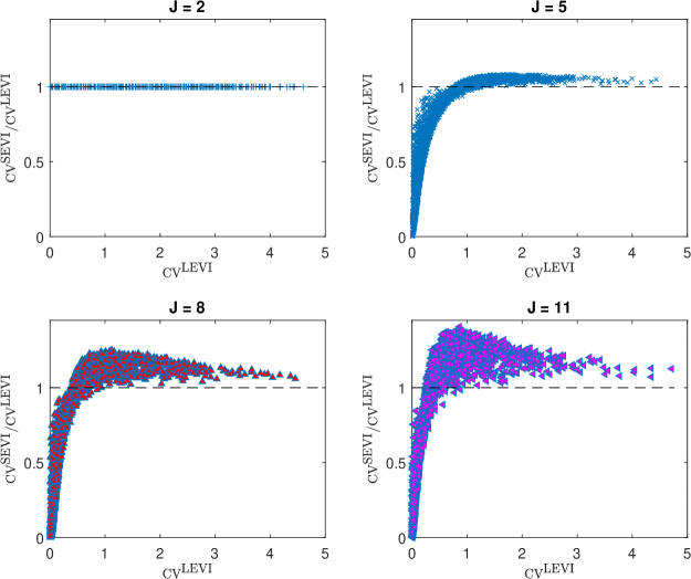
Figure 7: Scatter plot of the ratio of compensating variations in the SEVI and LEVI models $(\mathrm{CV}^{\mathrm{SEVI}}(k,V)/\mathrm{CV}^{\mathrm{LEVI}}(k,V))$ against the compensating variation in the LEVI model $(\mathrm{CV}^{\mathrm{LEVI}}(k,V))$ with the same DGPs as in Figure 3 ($X_{ij,\ell}$ is iid $N(0,\pi^{2}\omega_{j}^{2}/36))$

As a third application, we use Proposition 3 to establish the identification of a SEVI model. Note that the model under the vector of systematic utilities $V=(V_{1},\ldots,V_{J})$ is equivalent to that under $V^{o}=(V_{1}-V_{J},\ldots,V_{J-1}-V_{J},0)$, as the choice problem depends only on utility differences. For the purpose of studying identification, we normalize the systematic utility of the last alternative to zero and maintain this normalization in the rest of this subsection. Each vector of systematic utilities $V\in\mathbb{R}_{o}^{J}:=\mathbb{R}^{J-1}\otimes\left\{0\right\}$ maps into a vector of choice probabilities $P\in\mathbb{S}^{J-1}:=\{P=\left(P_{1},\ldots,P_{J-1}\right):P_{j}\geq 0$ and $\sum_{j=1}^{J-1}P_{j}\leq 1\}.$ The question remains whether we can deduce the systematic utilities from the choice probabilities.

Define the conjugate surplus function:

$$W_{\ast}^{\mathrm{SEVI}}\left(P\right):=\sup_{v\in\mathbb{R}_{o}^{J}}\left[\sum_{j=1}^{J-1}v_{j}P_{j}-W^{\mathrm{SEVI}}(v)\right]\text{ for any }P\in\mathbb{S}^{J-1}.$$

Since $W^{\mathrm{SEVI}}(v)$ is known and given in Proposition 3, it follows by construction that all of $W_{\ast}^{\mathrm{SEVI}}\left(\cdot\right):$ $\mathbb{S}^{J}\rightarrow\mathbb{R}$ and $\left\{\partial W_{\ast}^{\mathrm{SEVI}}\left(\cdot\right)/\partial P_{j}:\mathbb{S}^{J}\rightarrow\mathbb{R}\right\}_{j=1}^{J-1}$ are known functions. Using Theorem 7 of Sørensen and Fosgerau, (2022), we have:

$$V_{j}=\left.\frac{\partial W_{\ast}^{\mathrm{SEVI}}\left(P\right)}{\partial P_{j}}\right|_{P=\left[P^{\mathrm{SEVI}}(Y=1|V),\ldots,P^{\mathrm{SEVI}}\left(Y=J-1|V\right)\right]}$$

for $j=1,\ldots,J-1.$ That is, we can plug the vector of choice probabilities into $\left\{\partial W_{\ast}^{\mathrm{SEVI}}\left(\cdot\right)/\partial P_{j}\right\}_{j=1}^{J-1}$ to recover the vector of systematic utilities.

Given that the vector of choice probabilities is identified, the vector of systematic utilities is also identified. The problem of identifying the model parameter $\beta_{0}$ in a SEVI model reduces to the problem of identifying $\beta_{0}$ from the (joint) distribution of $V^{\ast}\left(\beta_{0}\right):=(V_{1}\left(\beta_{0}\right)-V_{J}\left(\beta_{0}\right),\ldots,V_{J-1}\left(\beta_{0}\right)-V_{J}\left(\beta_{0}\right))\in\mathbb{R}^{J-1}.$ Intuitively, if we have an infinite number of independent draws from the distribution of $V^{\ast}\left(\beta_{0}\right),$ can we pin down $\beta_{0}?$ Mathematically, if

$$\Pr(V^{\ast}\left(\beta_{1}\right)\neq V^{\ast}\left(\beta_{2}\right))>0\text{ for any }\beta_{1}\neq\beta_{2},$$ (18)

then $\beta_{0}$ is identified. This identification condition requires that, for two different model parameters, there is a positive probability that the resulting vectors of (normalized) systematic utilities are different. For example, in the linear case where $V_{i}^{\ast}\left(\beta\right)=\left[\left(X_{i1}-X_{iJ}\right)\beta,\ldots,\left(X_{iJ-1}-X_{iJ}\right)\beta\right],$ this requires that there is no perfect multicollinearity among the variables in $X_{ij}-X_{iJ}$ for at least one $j\in\left\{1,\ldots,J-1\right\}.$

The identification condition in (18) does not involve the distribution of $\varepsilon_{ij}.$ Therefore, it is applicable to any RUM model, provided that the unobserved random components $\left(\varepsilon_{i1},\ldots,\varepsilon_{iJ}\right)$ is independent of the systematic utility $\left(V_{i1},\ldots,V_{iJ}\right)$ and is absolutely continuous with full support $\mathbb{R}^{J}.$ See Corollary 1 of Sørensen and Fosgerau, (2022) for more discussions. In particular, this condition is applicable to a LEVI model. Hence, a SEVI model is identified if and only if the corresponding LEVI model is identified. No additional identification challenges arise in a SEVI model.

4 The MLE and QMLE of a SEVI Model

4.1 The Estimators

Consider the following conditional SEVI model

$$U_{ij}\left(\beta_{0}\right)=V_{ij}\left(\beta_{0}\right)+\varepsilon_{ij}\text{ and }V_{ij}\left(\beta_{0}\right)=X_{ij}\beta_{0}$$

for $j=1,\ldots,J$ where $X_{ij}\in\mathbb{R}^{L}$ and $\varepsilon_{ij}\thicksim iid$ $\mathrm{SEVI.}$ All other models in Remark 5 can be reformulated to take the above form. For example, if we want to include alternative-specific constants, we can introduce a dummy variable for each alternative and include the dummies for $\left(J-1\right)$ alternatives as part of $X_{ij}$. This dummy-variable method can also be used to allow for alternative-specific coefficients for any covariate, including individual-specific characteristics.

Given a simple random sample $\left\{Y_{i},X_{i1},\ldots,X_{iJ}\right\}_{i=1}^{n}$ from the above model, we consider estimating $\beta_{0}$ by MLE and QMLE. The MLE is the maximum likelihood estimator when the likelihood function is based on a correctly specified SEVI model, and the QMLE is the maximum likelihood estimator based on an incorrectly specified LEVI model.

The negative log-likelihood function of the model under the correct SEVI specification is

$$\ell_{\mathrm{SEVI}}\left(\beta\right)=\sum_{i=1}^{n}\ell_{i}^{\mathrm{SEVI}}\left(\beta\right)\text{ for }\ell_{i}^{\mathrm{SEVI}}\left(\beta\right)=-\sum_{k=1}^{J}Y_{ik}\log\left(P_{ik}^{\mathrm{SEVI}}\left(\beta\right)\right),$$

where $Y_{ik}:=1\left\{Y_{i}=k\right\}$ and $P_{ik}^{\mathrm{SEVI}}\left(\beta\right):=P^{\mathrm{SEVI}}\left(Y_{i}=k|v_{i}\left(\beta\right)\right)$ is defined as in (6) with $v_{i}$ replaced by $v_{i}\left(\beta\right).$ By minimizing the above negative log-likelihood function $\ell_{\mathrm{SEVI}}\left(\beta\right),$ we obtain the MLE:

$$\hat{\beta}_{\mathrm{MLE}}=\arg\min_{\beta\in\mathcal{B}}\ell_{\mathrm{SEVI}}\left(\beta\right),$$

where $\mathcal{B}$ is a large enough compact set in $\mathbb{R}^{L}.$

To compute the MLE, we can use a gradient-based algorithm. The gradient function is

$$\frac{\partial\ell_{\mathrm{SEVI}}\left(\beta\right)}{\partial\beta}=\sum_{i=1}^{n}\frac{\partial\ell_{i}^{\mathrm{SEVI}}\left(\beta\right)}{\partial\beta}:=\sum_{i=1}^{n}S_{i}^{\mathrm{SEVI}}\left(\beta\right),$$

where

$$S_{i}^{\mathrm{SEVI}}\left(\beta\right)=\sum_{j=1}^{J}\frac{\partial\ell_{i}^{\mathrm{SEVI}}\left(\beta\right)}{\partial v_{ij}\left(\beta\right)}\frac{\partial v_{ij}\left(\beta\right)}{\partial\beta}=-\sum_{j=1}^{J}\sum_{k=1}^{J}\frac{Y_{ik}}{P_{ik}^{\mathrm{SEVI}}\left(\beta\right)}\frac{\partial P_{ik}^{\mathrm{SEVI}}\left(\beta\right)}{\partial v_{ij}\left(\beta\right)}X_{ij}^{\prime}.$$

In the above, the expression of the derivative $\frac{\partial P_{ik}^{\mathrm{SEVI}}\left(\beta\right)}{\partial v_{ij}\left(\beta\right)}$ is given in (12) or (13) after plugging in the parameter $\beta.$ The closed-form expression for the gradient can be supplied to a gradient-based optimization algorithm.

Given the score $S_{i}^{\mathrm{SEVI}}\left(\beta\right)$ and the estimator $\hat{\beta}_{\mathrm{MLE}},$ we can estimate the asymptotic variance of $\hat{\beta}_{\mathrm{MLE}}$ by

$$\hat{\Omega}=\left[\frac{1}{n}\sum_{i=1}^{n}S_{i}^{\mathrm{SEVI}}(\hat{\beta}_{\mathrm{MLE}})S_{i}^{\mathrm{SEVI}}(\hat{\beta}_{\mathrm{MLE}})^{\prime}\right]^{-1}.$$

Following standard arguments, we can show that $\hat{\Omega}^{-1/2}\sqrt{n}(\hat{\beta}_{\mathrm{MLE}}-\beta_{0})\rightarrow^{d}N\left(0,I_{L}\right).$ Details are omitted here, as the theory is standard; See, for example, Chapter 13 of Wooldridge, (2002).

If we want to test $H_{0}:R\beta_{0}=r$ against $H_{1}:R\beta_{0}\neq r$ for some $q\times L$ matrix $R$ with row rank $q$ and $q\times 1$ vector $r,$ we can form the Wald statistic and show that it is asymptotically chi-squared under the null:

$$n\left(R\hat{\beta}_{\mathrm{MLE}}-r\right)\left(R\hat{\Omega}R^{\prime}\right)^{-1}\left(R\hat{\beta}_{\mathrm{MLE}}-r\right)\rightarrow^{d}\chi_{q}^{2}.$$

In particular, we can use the square root of the diagonal elements of $\left[\sum_{i=1}^{n}S_{i}^{\mathrm{SEVI}}(\hat{\beta}_{\mathrm{MLE}})S_{i}^{\mathrm{SEVI}}(\hat{\beta}_{\mathrm{MLE}})^{\prime}\right]^{-1}$, denoted by $\hat{\sigma}_{\ell},\ell=1,\ldots,L,$ as the standard errors for the elements of $\hat{\beta}_{\mathrm{MLE}}.$ We can construct a 95% confidence interval as $[\hat{\beta}_{\mathrm{MLE},\ell}-1.96\hat{\sigma}_{\ell},\hat{\beta}_{\mathrm{MLE},\ell}+1.96\hat{\sigma}_{\ell}].$

If the stochastic utilities follow SEVI, but we employ the maximum likelihood method under the incorrect assumption that they follow LEVI, we obtain the quasi-MLE (QMLE):

$$\hat{\beta}_{\mathrm{QMLE}} =\arg\min_{\beta\in\mathcal{B}}\ell_{\mathrm{LEVI}}\left(\beta\right)\text{ where }\ell_{\mathrm{LEVI}}\left(\beta\right)=\sum_{i=1}^{n}\ell_{i}^{\mathrm{LEVI}}\left(\beta\right)\text{ for }$$ (19)

$$\ell_{i}^{\mathrm{LEVI}}\left(\beta\right) =-\sum_{k=1}^{J}Y_{ik}\log\left(P_{ik}^{\mathrm{LEVI}}\left(\beta\right)\right)=-\sum_{k=1}^{J}Y_{ik}\left[X_{ik}\beta\right]-\log\left\{\sum_{j=1}^{J}\exp\left[X_{ij}\beta\right]\right\}.$$

The asymptotic properties of the QMLE are also standard results. In particular, we use the sandwich form for estimating the asymptotic variance of $\hat{\beta}_{\mathrm{QMLE}}$ when we know that the LEVI model is not the correct model.

4.2 On the Estimation of Parameter Ratios

Under some standard regularity conditions, $\hat{\beta}_{\mathrm{MLE}}$ is consistent for $\beta_{0},$ but in general, $\hat{\beta}_{\mathrm{QMLE}}$ is not. However, the ratio of the individual elements of $\hat{\beta}_{\mathrm{QMLE}}$, say $\hat{\beta}_{\mathrm{QMLE},2}/\hat{\beta}_{\mathrm{QMLE},1},$ may still be consistent for the true ratio, namely $\beta_{0,2}/\beta_{0,1},$ for a nonzero $\beta_{0,1}.$ In this subsection, we provide sufficient conditions for the consistency of the ratio estimator, even though the distribution of the random utility component is misspecified.

We consider an RUM with $V_{ij}\left(\beta_{0}\right)=X_{ij}\beta_{0}$ and specify $\varepsilon_{ij}\thicksim iid\mathrm{Q}$ for some distribution $\mathrm{Q}.$ This includes LEVI as an example but $\mathrm{Q}$ may be more general and incorrectly specified. Denote the choice probability derived under $\mathrm{Q}$ by $P^{\mathrm{Q}}(Y_{i}=k|V_{i}\left(\beta\right))$. Let $\beta_{\mathrm{Q}}^{\ast}$ be the pseudo-true value defined by

$$\beta_{\mathrm{Q}}^{\ast}=\arg\min_{\beta\in\mathcal{B}}-E\sum_{k=1}^{J}Y_{ik}\log P^{\mathrm{Q}}(Y_{i}=k|V_{i}\left(\beta\right)),$$

which is also the probability limit of $\hat{\beta}_{\mathrm{Q}}:=\arg\min_{\beta\in\mathcal{B}}-n^{-1}\sum_{i=1}^{n}\sum_{k=1}^{J}Y_{ik}\log P^{\mathrm{Q}}(Y_{i}=k|V_{i}\left(\beta\right)).$

We assume that $\beta_{\mathrm{Q}}^{\ast}$ is an interior point of the compact set $\mathcal{B}$ so that $\beta_{\mathrm{Q}}^{\ast}$ satisfies the first order zero-derivative conditions. The derivative of the population objective function with respect to $\beta$ is

$$-E\sum_{k=1}^{J}Y_{ik}\frac{\partial\log P^{\mathrm{Q}}(Y_{i}=k|\mathcal{J},V_{i}\left(\beta\right))}{\partial\beta}=-EX_{i}^{\prime}\sum_{k=1}^{J}Y_{ik}\lambda_{ik}^{\mathrm{Q}}\left(X_{i}\beta\right)=-EX_{i}^{\prime}\Lambda_{i}^{\mathrm{Q}}\left(X_{i}\beta\right)\overrightarrow{Y}_{i},$$

where

$$X_{i} =(X_{i1}^{\prime},\ldots,X_{iJ}^{\prime})^{\prime}\in\mathbb{R}^{J\times L},$$

$$\lambda_{ik}^{\mathrm{Q}}\left(X_{i}\beta\right) =\left.\frac{\partial\log P^{\mathrm{Q}}(Y_{i}=k|\mathcal{J},V_{i}=v_{i})}{\partial v_{i}}\right|_{v_{i}=X_{i}\beta}\in\mathbb{R}^{J\times 1},$$

$$\Lambda_{i}^{\mathrm{Q}}\left(X_{i}\beta\right) =\left[\lambda_{i1}^{\mathrm{Q}}\left(X_{i}\beta\right),\ldots,\lambda_{iJ}^{\mathrm{Q}}\left(X_{i}\beta\right)\right]\in\mathbb{R}^{J\times J},\text{ }\overrightarrow{Y}_{i}=(Y_{i1},\ldots,Y_{iJ})^{\prime}\in\mathbb{R}^{J\times 1}.$$

So, $\beta_{\mathrm{Q}}^{\ast}$ satisfies $E\left[X_{i}^{\prime}\Lambda_{i}^{\mathrm{Q}}(X_{i}\beta_{\mathrm{Q}}^{\ast})\overrightarrow{Y}_{i}\right]=0.$

Proposition 4

Assume that (i) $\hat{\beta}_{\mathrm{Q}}\rightarrow^{p}\beta_{\mathrm{Q}}^{\ast}\in Int(\mathcal{B)}$, and $\beta_{\mathrm{Q}}^{\ast}$ is the unique solution to $E\left[X_{i}^{\prime}\Lambda_{i}^{\mathrm{Q}}\left(X_{i}\beta\right)\overrightarrow{Y}_{i}\right]=0;$

(ii) $\beta_{0}\neq 0$, and there exists a nonzero scalar $\delta_{1}^{\circ}$ such that $E\left[X_{i}^{\prime}\Lambda_{i}^{\mathrm{Q}}\left(X_{i}\beta_{0}\delta_{1}^{\circ}\right)\overrightarrow{Y}_{i}\right]=0;$

(iii) $E\left[X_{i,j,\ell}|X_{i1}\beta_{0},X_{i2}\beta_{0},\ldots,X_{iJ}\beta_{0}\right]=\Theta_{0,\ell}+\left(X_{ij}\beta_{0}\right)\Theta_{1,\ell}$ for some scalars $\Theta_{0,\ell}$ and $\Theta_{1,\ell}$ and for $\ell=2,\ldots,L.$

Then: $\beta_{\mathrm{Q}}^{\ast}=\delta_{1}^{\circ}\beta_{0}.$

Proposition 4 shows that while the QMLE $\hat{\beta}_{\mathrm{Q}}$ may not be consistent for $\beta_{0}$, it converges to $\beta_{0}$ up to a multiplicative factor. In particular, if $\beta_{0,m_{1}}\neq 0,$ then

$$\frac{\hat{\beta}_{\mathrm{Q,}m_{2}}}{\hat{\beta}_{\mathrm{Q,}m_{1}}}\rightarrow^{p}\frac{\beta_{0,m_{2}}}{\beta_{0,m_{1}}}.$$

This says that the plug-in ratio estimator is consistent for the true ratio.

Assumption (iii) in Proposition 4 holds if $X_{i1},\ldots,X_{iJ}$ are independent and each follows a multivariate normal or elliptical distribution. The latter assumption is sufficient but not necessary. There may exist other distributions of $X_{i1},\ldots,X_{iJ}$ or specific ways to relax the independence assumption such that the proportionality result holds. In empirical applications, the ratio estimator could still be close to the true ratio even though Assumption (iii) does not hold.

Proposition 4 is proved along the lines of the proof of Theorem 1 in Ruud, (1986), which does not cover multinomial choice models. Some adjustments to the proof in Ruud, (1986) are needed to account for two main differences: there is no constant term in a multinomial choice model and the covariate $X_{i}$ in this model is a matrix rather than a vector.

4.3 The Choice between SEVI and LEVI

In empirical applications, it is often the case that neither the SEVI nor the LEVI is correctly specified. However, we still have to decide which model to use. To aid in this decision, we can employ the Akaike Information Criterion (AIC) or the Bayesian Information Criterion (BIC). Since both models have the same number of parameters, we can compare their empirical (quasi) log-likelihoods, which leads to the likelihood ratio statistic given by

$$\mathrm{LR} :=\ell_{\mathrm{SEVI}}(\hat{\beta}_{\mathrm{SEVI}})-\ell_{\mathrm{LEVI}}(\hat{\beta}_{\mathrm{LEVI}})$$

$$=\sum_{i=1}^{n}\left[\ell_{i}^{\mathrm{SEVI}}\left(\hat{\beta}_{\mathrm{SEVI}}\right)-\ell_{i}^{\mathrm{LEVI}}\left(\hat{\beta}_{\mathrm{LEVI}}\right)\right].$$

Note that in the previous section, $\hat{\beta}_{\mathrm{SEVI}}$ and $\hat{\beta}_{\mathrm{LEVI}}$ were denoted as $\hat{\beta}_{\mathrm{MLE}}$ and $\hat{\beta}_{\mathrm{QMLE}},$ respectively. However, in this section, both the SEVI model and the LEVI model can be misspecified and so both $\hat{\beta}_{\mathrm{SEVI}}$ and $\hat{\beta}_{\mathrm{LEVI}}$ can be quasi-maximum likelihood estimators.

In empirical applications, the choice between the SEVI model and the LEVI model can be based on the likelihood ratio. If $\mathrm{LR}>0$, then the LEVI model is preferred. Conversely, if $\mathrm{LR}<0$, then the SEVI model is preferred. This simple empirical rule of thumb is derived from the empirical goodness of fit and serves as a practical guide for selecting between the two models. It is worth pointing out again that this rule is also the model selection rule based on the AIC or BIC, as the two models have the same number of parameters.

Another method to determine which model to use is by employing Vuong’s test (Vuong, (1989)), which formally assesses the null hypothesis that the SEVI model and the LEVI model provide equally good fits to the data. Let $\beta_{\mathrm{SEVI}}^{\ast}$ and $\beta_{\mathrm{LEVI}}^{\ast}$ be the respective limits of $\hat{\beta}_{\mathrm{SEVI}}$ and $\hat{\beta}_{\mathrm{LEVI}}$. In the present setting, the null hypothesis of Vuong’s test can be expressed as:

$$H_{0}:E\left[\ell_{\mathrm{SEVI}}\left(\beta_{\mathrm{SEVI}}^{\ast}\right)|V\right]=E\left[\ell_{\mathrm{LEVI}}\left(\beta_{\mathrm{LEVI}}^{\ast}\right)|V\right]$$

almost surely, where $V$ is the vector collecting the systematic utilities. Note that

$$E\left[\ell_{\mathrm{SEVI}}\left(\beta_{\mathrm{SEVI}}^{\ast}\right)|V\right]=-\sum_{k=1}^{J}P_{ik}^{o}\log\left(P_{ik}^{\mathrm{SEVI}}\left(\beta_{\mathrm{SEVI}}^{\ast}\right)\right)$$

where $P_{ik}^{o}:=\Pr(Y_{i}=k|V_{i})$ is the true choice probability. The right-hand side of the above equation is the cross entropy between $\left(P_{i1}^{0},\ldots,P_{iJ}^{o}\right)$ and ($P_{i1}^{\mathrm{SEVI}}\left((\beta_{\mathrm{SEVI}}^{\ast}\right),\ldots,P_{iJ}^{\mathrm{SEVI}}\left(\beta_{\mathrm{SEVI}}^{\ast}\right)$), which quantifies the difference between these two distributions. By adding a constant $\sum_{k=1}^{J}P_{ik}^{o}\log\left(P_{ik}^{o}\right)$ to both sides, we have

$$E\left[\ell_{\mathrm{SEVI}}\left(\beta_{\mathrm{SEVI}}^{\ast}\right)|V\right]+\sum_{k=1}^{J}P_{ik}^{o}\log\left(P_{ik}^{o}\right)=-\sum_{k=1}^{J}P_{ik}^{o}\log\left(\frac{P_{ik}^{\mathrm{SEVI}}\left(\beta_{\mathrm{SEVI}}^{\ast}\right)}{P_{ik}^{o}}\right),$$

where the right-hand side is the KL distance between the two distributions $\left(P_{i1}^{0},\ldots,P_{iJ}^{o}\right)$ and ($P_{i1}^{\mathrm{SEVI}}\left(\beta_{\mathrm{SEVI}}^{\ast}\right),\ldots,P_{iJ}^{\mathrm{SEVI}}\left(\beta_{\mathrm{SEVI}}^{\ast}\right)$) conditional on $V.$ Similar calculations can be performed for $E\left[\ell_{\mathrm{LEVI}}\left(\beta_{\mathrm{LEVI}}^{\ast}\right)|V\right].$ Therefore, the null of Vuong’s test is that the SEVI and LEVI models are equidistant from the true data generating process, with the “distance” measured by either the cross-entropy or the KL distance.

Since the SEVI model and the LEVI model are nonnested, $n^{-1/2}\left[\ell_{\mathrm{SEVI}}(\hat{\beta}_{\mathrm{SEVI}})-\ell_{\mathrm{LEVI}}(\hat{\beta}_{\mathrm{LEVI}})\right]$ is asymptotically normal. We can standardize the LR statistic to obtain the $\mathcal{V}_{n}$ statistic of Vuong, (1989):

$$\mathcal{V}_{n}=\frac{\sum_{i=1}^{n}\left[\ell_{i}^{\mathrm{SEVI}}\left(\hat{\beta}_{\mathrm{SEVI}}\right)-\ell_{i}^{\mathrm{LEVI}}\left(\hat{\beta}_{\mathrm{LEVI}}\right)\right]}{\left\{\sum_{i=1}^{n}\left[\ell_{i}^{\mathrm{SEVI}}\left(\hat{\beta}_{\mathrm{SEVI}}\right)-\ell_{i}^{\mathrm{LEVI}}\left(\hat{\beta}_{\mathrm{LEVI}}\right)-n^{-1}\mathrm{LR}\right]^{2}\right\}^{1/2}}.$$

Following the arguments in Vuong, (1989), we can show that under the null $\mathcal{V}_{n}\rightarrow^{d}N(0,1).$ This serves as the basis for both one-sided tests and two-sided tests. For example, if $\left|\mathcal{V}_{n}\right|>1.96,$ then we may reject the null that the SEVI and LEVI models fit the data equally well at the 5% significance level. On the other hand, if $\mathcal{V}_{n}>1.645,$ we may reject the null that the SEVI model fits the data better at the 5% significance level. If $\mathcal{V}_{n}<-1.645,$ we may reject the null that the LEVI model fits the data better at the 5% significance level.

5 Simulation Evidence

We generate the data from a conditional SEVI model. More specifically, we assume that

$$Y_{i}=\arg\max_{j=1,\ldots,J}\left\{X_{ij}\beta+\varepsilon_{ij}\right\}$$

where $\varepsilon_{ij}\thicksim iid$ SEVI over $j$ and $X_{ij,\ell}\thicksim iidN(0,\pi^{2}\omega_{j}^{2}/36)$ or $X_{ij,\ell}\thicksim iidN(0,\pi^{2}/36)$ over $\ell=1,2$ and $3$. The DGPs are the same as the SEVI DGPs in Figures 3–5. Given a simple random sample $\left\{Y_{i},X_{i1},\ldots,X_{iJ}\right\}_{i=1}^{n},$ we use the MLE and QMLE in Section 4 to estimate $\beta_{0}=\left(1,2,1\right)^{\prime}.$ To reiterate, the MLE is based on the correct specification that $\varepsilon_{ij}\thicksim iid$ SEVI, and the QMLE is based on the incorrect specification that $\varepsilon_{ij}$ $\thicksim iid$ LEVI.

5.1 Simulation with a Large Sample Size

We first consider the case that the sample size is large, and there is only one simulation replication. The purpose of this exercise is to see how large the misspecification bias is. Table 1 reports the estimates when the sample size $n$ is $10,000.$ When $J=2,$ the MLE and QMLE give the same estimate of $\beta_{0}.$ This is consistent with the result that the SEVI model and the LEVI model are the same when there are only two alternatives. When $J>2,$ the MLE and QMLE are quite different. While the MLE is close to the true parameter vector for all values of $J$ considered, the QMLE grows with $J.$ For example, when $J=8$ and $X_{ij,\ell}\thicksim iidN(0,\pi^{2}\omega_{j}^{2}/36),$ the QMLE is $\left(1.48,2.99,1.49\right)$, each element of which is higher than the corresponding true value by about 50%. The misspecification bias of the QMLE is substantial. In line with Proposition 4, the ratio of the estimates of any two elements of $\beta_{0}$, say $\hat{\beta}_{\mathrm{QMLE},2}/\hat{\beta}_{\mathrm{QMLE},1},$ is close to the true ratio $\beta_{0,2}/\beta_{0,1}.$ This is true regardless of whether the attributes have the same variance across the alternatives or not. Proposition 4 permits variance heterogeneity across the alternatives.

	True		$J=2$			$J=5$			$J=8$			$J=11$
	$(\boldsymbol{\beta}_{\boldsymbol{0}})$		MLE	QMLE		MLE	QMLE		MLE	QMLE		MLE	QMLE
			$X_{ij,\ell}\thicksim iidN(0,\pi^{2}\omega_{j}^{2}/36)$
$\beta_{1}$	1.00		1.01	1.01		1.00	1.37		0.98	1.48		1.02	1.64
$\beta_{2}$	2.00		1.95	1.95		2.01	2.75		1.99	2.99		1.98	3.17
$\beta_{3}$	1.00		0.99	0.99		1.00	1.37		1.01	1.49		0.98	1.57
			$X_{ij,\ell}\thicksim iidN(0,\pi^{2}/36)$
$\beta_{1}$	1.00		1.01	1.01		1.01	1.35		0.99	1.51		1.00	1.64
$\beta_{2}$	2.00		2.03	2.03		2.05	2.80		1.98	3.09		1.98	3.37
$\beta_{3}$	1.00		1.03	1.03		1.03	1.38		1.03	1.56		1.00	1.64

Table 1: MLE and QMLE of the model parameters for various J

In a nonlinear model, instead of focusing on the parameter values, it can be more informative to examine the (empirical) average partial effects, defined by

$$APE(j;\beta,\mathrm{SEVI}) =\frac{1}{n}\sum_{i=1}^{n}\frac{\partial P_{ij}^{\mathrm{SEVI}}\left(\beta\right)}{\partial X_{ij,1}}=\frac{1}{n}\sum_{i=1}^{n}\frac{\partial P_{ij}^{\mathrm{SEVI}}\left(\beta\right)}{\partial v_{ij}\left(\beta\right)}\beta_{1},$$

$$APE(j;\beta,\mathrm{LEVI}) =\frac{1}{n}\sum_{i=1}^{n}\frac{\partial P_{ij}^{\mathrm{LEVI}}\left(\beta\right)}{\partial X_{ij,1}}=\frac{1}{n}\sum_{i=1}^{n}P_{ij}^{\mathrm{LEVI}}\left(\beta\right)\left(1-P_{ij}^{\mathrm{LEVI}}\left(\beta\right)\right)\beta_{1}.$$

In the above, $P_{ij}^{\mathrm{SEVI}}$ and $P_{ij}^{\mathrm{LEVI}}$ are the choice probabilities under the SEVI and LEVI specifications, respectively. $APE(j;\beta,\mathrm{SEVI})$ and $APE(j;\beta,\mathrm{LEVI})$ are the corresponding empirical APEs that measure the effect on the probability of choosing alternative $j$ when a marginal change is made to one of alternative $j$’s attributes. We focus on the first attribute $X_{ij,1}$ and plot the ratios:

$$\frac{APE(j;\hat{\beta}_{\mathrm{MLE}},\mathrm{SEVI})}{APE(j;\beta_{0},\mathrm{SEVI})}\text{ and }\frac{APE(j;\hat{\beta}_{\mathrm{QMLE}},\mathrm{LEVI})}{APE(j;\beta_{0},\mathrm{SEVI})}$$

against the label of each alternative $j=1,\ldots,J.$ Figure 8 reports the results for the case that $X_{ij,\ell}\thicksim iidN(0,\pi^{2}\omega_{j}^{2}/36)$ and makes it clear that the empirical APE is not close to the target APE (i.e., $APE(j;\beta_{0},\mathrm{SEVI})$) when the model is misspecified. This shows that the difference in the parameter estimates due to model misspecification has substantial effects on APE estimation.

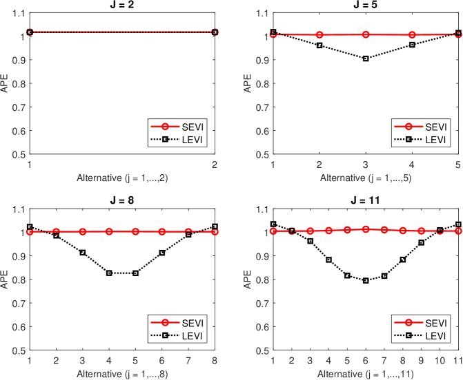
Figure 8: Plots of the empirical APE under the correct SEVI specification and the incorrect LEVI specification against alternative labels for a sample of $n=10,000$ individuals

To further illustrate the difference between the SEVI and LEVI specifications, we conduct an out-of-sample prediction exercise. Let $\hat{\beta}_{\mathrm{MLE}}^{\left(J\right)}$ and $\hat{\beta}_{\mathrm{QMLE}}^{\left(J\right)}$ be the MLE and QMLE of $\beta_{0}$, respectively, when there are $J$ alternatives. We use $\hat{\beta}_{\mathrm{MLE}}^{\left(J\right)}$ and $\hat{\beta}_{\mathrm{QMLE}}^{\left(J\right)}$ to compute out-of-sample choice probabilities for a certain choice problem. More specifically, we assume that an out-of-sample individual chooses between the first two alternatives only, and the rest $J-2$ alternatives are not available. In this case, the out-of-sample choice probabilities are

$$\hat{P}_{i_{o},\mathrm{MLE}}:=P\left(Y_{i_{o}}=1|X_{i_{o}};\hat{\beta}_{\mathrm{MLE}}^{\left(J\right)}\right)\text{ and }\hat{P}_{i_{o},\mathrm{QMLE}}=P\left(Y_{i_{o}}=1|X_{i_{o}};\hat{\beta}_{\mathrm{QMLE}}^{\left(J\right)}\right)$$

where

$$P\left(Y_{i_{o}}=1|X_{i_{o}};\beta\right)=\frac{\exp(X_{i_{o},1}\beta)}{\exp(X_{i_{o},1}\beta)+\exp(X_{i_{o},2}\beta)}$$

and $i_{o}\in\left\{n+1,\ldots,2n\right\}$ represents an out-of-sample individual whose observation $(X_{i_{o}},Y_{i_{o}})$ was not used in constructing the MLE or QMLE, but $\left(X_{i_{o}},Y_{i_{o}}\right)$ is generated in the same way as any in-sample observation. Note that the number of “out-of-sample” individuals is the same as the number of “in-sample” individuals and both are equal to 10,000.

When there are only two alternatives in the out-of-sample prediction exercise, the formulae for the choice probabilities are the same under SEVI or LEVI. Hence, as given above, $\hat{P}_{i_{o},\mathrm{MLE}}$ and $\hat{P}_{i_{o},\mathrm{QMLE}}$ are different only because they are based on different estimated parameters.

Figure 9(a&b) reports the kernel density estimators (KDE) of $\left\{P\left(Y_{i_{o}}=1|X_{i_{o}};\beta\right)\right\}_{i=n+1}^{2n}$ for $\beta=\beta_{0},\hat{\beta}_{\mathrm{MLE}}^{\left(J\right)}$ and $\hat{\beta}_{\mathrm{QMLE}}^{\left(J\right)}$ when $J=5$ and $X_{ij,\ell}\thicksim iidN(0,\pi^{2}\omega_{j}^{2}/36).$ It is not surprising that the KDE under $\hat{\beta}_{\mathrm{MLE}}^{\left(J\right)}$ is very close to the target KDE, that is, the KDE under $\beta_{0}.$ When the sample size is large, $\hat{\beta}_{\mathrm{MLE}}^{\left(J\right)}$ is very close to $\beta_{0}$, as demonstrated in Table 1. As a result, $P(Y_{i_{o}}=1|X_{i_{o}};\hat{\beta}_{\mathrm{MLE}}^{\left(J\right)})$ is close to $P\left(Y_{i_{o}}=1|X_{i_{o}};\beta_{0}\right)$ and therefore, the corresponding KDEs are close to each other. On the other hand, the KDE under $\hat{\beta}_{\mathrm{QMLE}}^{\left(J\right)}$ is quite different from the target KDE. This demonstrates that the model misspecification introduces not only a significant bias in the parameter estimator but also a substantial discrepancy in the predicted choice probabilities.

The KDE figure for the case that $J=5$ and $X_{ij,\ell}\thicksim iidN(0,\pi^{2}/36)$ is qualitatively similar to Figure 9(a&b) and is thus omitted. The KDE figure for the case that $J=11$ and $X_{ij,\ell}\thicksim iidN(0,\pi^{2}\omega_{j}^{2}/36)$ is reported in Figure 9(c&d). The difference between the KDE under $\hat{\beta}_{\mathrm{QMLE}}^{(J)}$ and the target KDE appears to increase with $J.$

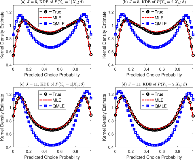
Figure 9: Kernel density estimation of the out-of-sample predictive probabilities when $n=10,000,J=5,11$ and $X_{ij,\ell}\thicksim iidN(0,\pi^{2}\omega_{j}^{2}/36)$

As final evidence that it matters whether the stochastic utility follows the SEVI or LEVI distribution, we compute the out-of-sample predicted choice probabilities when there are four alternatives $(J=4)$ for both the in-sample estimation and out-of-sample prediction. For the latter, we compute $\hat{P}_{i_{o},\mathrm{MLE}}^{\mathrm{SEVI}}(j):=P(Y_{i_{o}}=j|X_{i_{o}};\mathrm{SEVI},$ $\hat{\beta}_{\mathrm{MLE}}^{\left(4\right)})$ and $\hat{P}_{i_{o},\mathrm{QMLE}}^{\mathrm{LEVI}}\left(j\right):=P(Y_{i_{o}}=j|X_{i_{o}};\mathrm{LEVI},\hat{\beta}_{\mathrm{QMLE}}^{\left(4\right)})$ where we have emphasized the dependence of the choice probability on the distributional assumption imposed on the stochastic utility. We plot the difference $\hat{P}_{i_{o},\mathrm{MLE}}^{\mathrm{SEVI}}(j)-\hat{P}_{i_{o},\mathrm{QMLE}}^{\mathrm{LEVI}}(j)$ against the true choice probability $P_{i_{o},0}^{\mathrm{SEVI}}(j):=P(Y_{i_{o}}=j|X_{i_{o}};\mathrm{SEVI},$ $\beta_{0})$ as a scatter plot. We omit the figure here, but it is available as Figure S.7 in the supplementary appendix. The figure clearly shows that, relative to the true choice probability, the difference can be substantial.

5.2 Simulation with Smaller Sample Sizes

In this subsection, we study the performances of MLE and QMLE in finite samples. Using the same DGP as in the previous subsection, we consider the sample size $n=500$, $1000$ and the number of alternatives $J=2,5,8,11.$ The number of simulation replications is 5000. For each estimator, we compute the bias, the empirical standard derivation, and the average of the standard errors across the simulation replications. Furthermore, we construct a 95% confidence interval for each element of $\beta_{0}$ following the standard procedure of adding and subtracting 1.96 times the standard error and report the empirical coverage of the CI (i.e., the proportion of times the so-constructed confidence interval contains the true parameter value).

Table 2 reports the results when $X_{ij,\ell}\thicksim iidN(0,\pi^{2}\omega_{j}^{2}/36)$ and $n=500$. The reported results are representative of other cases with a different DGP for $X_{ij,\ell}$ or sample size. A few patterns emerge. First, the bias of the MLE is small and decreases with $J.$ On the other hand, the bias of the QMLE is large and increases with $J.$ This is consistent with our large sample result when $n=10,000$ and there is only one simulation replication. Here, the finite sample biases (with $n=500$) are averaged over 5000 simulation replications. Second, for both the MLE and QMLE, the empirical standard deviation decreases with $J.$ A larger $J$ can be regarded as having more observations and, hence, smaller sampling noises. Third, for both estimators, the average of the standard errors across the simulation replications matches with the corresponding standard deviation very well. This indicates that the standard errors are reliable estimates of the standard deviation. Finally, for the MLE, the empirical coverage of the 95% confidence intervals is very close to 95%. This shows that the asymptotic normal approximation is reliable. On the other hand, for the QMLE, the empirical coverage of the 95% confidence intervals is much smaller than 95%. The only exception is the case when $J=2$, where MLE and QMLE are identical. In this case, there is a small and nearly invisible difference in the empirical coverages, because the standard error for the MLE is based on the non-robust asymptotic variance estimator while the standard error for the QMLE is based on the robust sandwich asymptotic variance estimator. Both variance estimators are consistent when $J=2.$ When $J>2,$ the under-coverage of the CIs based on the QMLE is due to the bias in the QMLE. The larger the number of alternatives $J$ is, the larger the bias is, and the smaller the empirical coverage is.

	MLE					QMLE
	Empirical	Empirical	Average of	Empirical		Empirical	Empirical	Average of	Empirical
	Bias	StD	SE’s	Coverage		Bias	StD	SE’s	Coverage
	$J=2$
$\beta_{1}$	0.009	0.211	0.210	0.951		0.009	0.211	0.209	0.948
$\beta_{2}$	0.023	0.240	0.241	0.950		0.023	0.240	0.239	0.950
$\beta_{3}$	0.010	0.209	0.210	0.950		0.010	0.209	0.209	0.950
	$J=5$
$\beta_{1}$	0.003	0.105	0.107	0.957		0.366	0.141	0.142	0.261
$\beta_{2}$	0.010	0.136	0.137	0.950		0.738	0.175	0.173	0.004
$\beta_{3}$	0.004	0.106	0.107	0.958		0.367	0.142	0.142	0.266
	$J=8$
$\beta_{1}$	0.006	0.087	0.088	0.952		0.514	0.130	0.129	0.017
$\beta_{2}$	0.011	0.117	0.116	0.951		1.026	0.159	0.158	0.000
$\beta_{3}$	0.006	0.088	0.088	0.951		0.513	0.129	0.129	0.017
	$J=11$
$\beta_{1}$	0.004	0.080	0.080	0.950		0.600	0.124	0.123	0.000
$\beta_{2}$	0.007	0.105	0.107	0.955		1.201	0.149	0.150	0.000
$\beta_{3}$	0.007	0.081	0.080	0.946		0.605	0.126	0.123	0.001

Table 2: Finite sample performances of the MLE and QMLE

Next, we consider testing IIA using the case when $X_{ij,\ell}\thicksim iidN(0,\pi^{2}/36),\ell=1,2,3$ and $n=500$ as an example. We follow the standard procedure to perform the Hausman-McFadden test (cf., Hausman and McFadden, (1984)). For each simulation replication, we first estimate the model under the (incorrect) LEVI specification using the full sample. We then carry out the same estimation procedure but use only the subsample of individuals who choose either alternative 1 or 2. We compare these two estimates using the Wald statistic based on the 95% critical value from the chi-squared distribution with three degrees of freedom ($\chi^{2}(3)$). The empirical rates of rejection over 5000 simulation replications for $J=5,8,$ and $11$ are 30.30%, 40.18%, and 47.52%, respectively. This indicates a fairly good chance of the IIA being rejected. Following an IIA rejection, the standard practice is to employ discrete choice models that do not exhibit the IIA property, such as the mixed logit. However, in the present setting, such a practice would lead to a wrong characterization of agents’ preferences.

We note that the LEVI model is misspecified for both the full sample and the subsample of the individuals who choose either alternative 1 or 2. The misspecification of the LEVI model for the full sample is obvious as the stochastic utility follows the SEVI distribution rather than the LEVI distribution. For the subsample with the two alternatives selected by the econometrician, the LEVI model is still misspecified. From the point of view of the econometrician, the conditional probability of choosing alternative 1 given that either alternative 1 or alternative 2 is chosen is

$$\frac{\Pr(Y=1|\mathcal{J},V=v,\varepsilon_{j}\thicksim iid\text{ }\mathrm{SEVI}\text{ over }j\in\mathcal{J})}{\Pr(Y=1|\mathcal{J},V=v,\varepsilon_{j}\thicksim iid\text{ }\mathrm{SEVI}\text{ over }j\in\mathcal{J})+\Pr(Y=2|\mathcal{J},V=v,\varepsilon_{j}\thicksim iid\text{ }\mathrm{SEVI}\text{ over }j\in\mathcal{J})}.$$ (20)

This is not equal to $\exp(v_{1})/[\exp(v_{1})+\exp(v_{2})]$ unless $\mathcal{J}=\left\{1,2\right\}.$ However, the Hausman–McFadden test requires at least three alternatives in total, as otherwise the test statistic equals zero and the IIA null is never rejected. So, whenever the Hausman-McFadden test is meaningful, the LEVI model is misspecified for any subsample with at least two alternatives.

Finally, we consider using Vuong’s test and AIC/BIC to decide which model fits the data better. When the SEVI is the correct model, $X_{ij,\ell}\thicksim iidN(0,\pi^{2}\omega_{j}^{2}/36)$ and $n=500$, the fractions of the test statistic $\mathcal{V}_{n}$ less than $-1.645$ across 5000 simulation replications are 47.08%, 69.08, and 80.82%, respectively, for $J=5,8,$ and $11$. The corresponding fractions of the test statistic less than $0$ are 92.56%, 97.86%, and 99.32%, respectively. These results underscore the reasonable power of Vuong’s test and the high accuracy of the AIC/BIC in selecting the correct SEVI model. Results are similar when $X_{ij,\ell}\thicksim iidN(0,\pi^{2}/36)$ and for other sample sizes. On the other hand, when the LEVI is the correct model, $X_{ij,\ell}\thicksim iidN(0,\pi^{2}\omega_{j}^{2}/36)$ and $n=500$, we observe that the test statistic $\mathcal{V}_{n}$ exceeds 1.645 in 30.58%, 48.22%, and 60.72% of the cases across 5000 simulation replications for $J=5,8,$ and $11$, respectively. The corresponding percentages for $\mathcal{V}_{n}$ greater than zero are 87.56%, 94.94%, and 97.18% for $J=5,8,$ and $11$, respectively. This affirms the power of Vuong’s test and the effectiveness of using the AIC/BIC in selecting the correct LEVI model. Therefore, regardless of whether the SEVI or LEVI model is the true model, Vuong’s test has good power and the AIC and BIC perform very well in correctly identifying the true model.

5.3 Computation Time Comparison

In this subsection, we compare the computation times required for estimating the LEVI and SEVI models. Additionally, we include the multinomial probit model with iid normal errors with variance $\pi^{2}/6$ in our comparison. For the sake of uniformity with the nomenclature used for the other two models, we will henceforth refer to this restricted multinomial probit model as the NORM model.

The data are generated according to $Y_{i}=\max_{j=1}^{J}\left\{X_{ij}\beta+\varepsilon_{ij}\right\}$ where $X_{ij,\ell}\thicksim iidN(0,\pi^{2}\omega_{j}^{2}/36)$ over $\ell=1,\ldots,L$ (cf., equation (10)) and $\varepsilon_{ij}\thicksim iid$ $\mathrm{SEVI}$ over $j.$ We fit the LEVI, SEVI, NORM models to the so-generated data. All models have the same correct linear specification $V_{ij}\left(\beta\right)=X_{ij}\beta$ for the systematic utility but differ with respect to the distributional specification of the random components.

We use a sample size of 1000, explore different numbers of alternatives $(J)$ ranging from 2 to 16, and consider two different numbers of attributes $(L=3$ and $L=10)$. To mimic real data analysis, we simulate only one sample with model parameter $\beta_{0}$ drawn randomly from a multivariate standard normal distribution.

We document the time needed to obtain the ML/QML estimate of the model parameters for each of the three models. The time represents the seconds spent by our MATLAB program to find each point estimate. All computations are performed on a desktop PC equipped with an Intel i7-13700F processor and 32GB of RAM. While no parallel method is employed, we strive to vectorize all operations as much as possible. For the SEVI model, the choice probabilities are computed using the formula in Theorem 1. In the case of the NORM model, the choice probabilities are obtained using the Geweke–Hajivassiliou–Keane (GHK) simulator with 500 simulations (Geweke and Keane, (2001); Hajivassiliou and McFadden, (1998); Keane and Wolpin, (1994)).

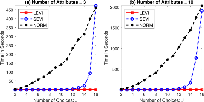
Figure 10: Comparison of computation times for the LEVI, SEVI, and NORM (MNP with $\varepsilon_{ij}\thicksim iidN(0,\pi^{2}/6))$ models when $V_{ij}=X_{ij}\beta$

Figure 10 plots the computation time against the number of alternatives. On one hand, when $J\leq 12,$ the computation time for the SEVI model is comparable to that for the LEVI model. When $J>12$, the computation time for the SEVI model starts to increase with $J$ and becomes significantly larger than that for the LEVI model, especially when $J$ reaches $16.$ On the other hand, when $J\leq 12,$ the NORM model exhibits a clear computational disadvantage compared to the LEVI and SEVI models. While the computation time for each of the latter two models is less than 27 seconds when the number of attributes is 10 and the number of alternatives is 12, the corresponding computation time for the NORM model is more than 1000 seconds. In our experiment, the SEVI model starts to become computationally as costly as the NORM model only when $J=16.$

While the first DGP contains no alternative specific constant, the second group of DGPs we consider does. We examine two scenarios: one with only alternative-specific constants where $V_{ij}=Z_{i}\beta_{zj}$ for $Z_{i}=1$ (hereafter, ASC-only) and another with alternative-specific constants $\left(Z_{i}\right)$ and three attributes $X_{ij,\ell}\thicksim iidN(0,\pi^{2}\omega_{j}^{2}/36),\ell=1,2,3$. In the latter case, $V_{ij}=Z_{i}\beta_{zj}+X_{ij,1}\beta_{x1}+X_{ij,2}\beta_{x2}+X_{ij,3}\beta_{x3}$ where $Z_{i}=1.$ In both cases, $\varepsilon_{ij}\thicksim iid$ $\mathrm{SEVI}$ over $j=1,\ldots,J.$ For each dataset, we fit the LEVI, SEVI, and NORM models with correctly specified system utility. Figure 11 reports the computation times. The general patterns observed in Figure 10 carry over to this figure. When $J\leq 12,$ the SEVI and LEVI models require less than 65 seconds for estimation, with much shorter times for a smaller $J.$ In contrast, the time needed for the NORM model grows rapidly as $J$ increases from 2 to 12. For example, when $J=10$ and $12,$ the required times for the NORM model for the ASC-only case are 2274 and 5159 seconds, respectively. In other words, estimating a standard multinomial probit model takes between half an hour and two hours when $J$ is about 10 or 12, whereas the corresponding time for a SEVI model is just about 1 minute. As before, the SEVI model becomes computationally less competitive for $J>12$ and has a computational cost starting to approach the NORM model when $J$ reaches 16.

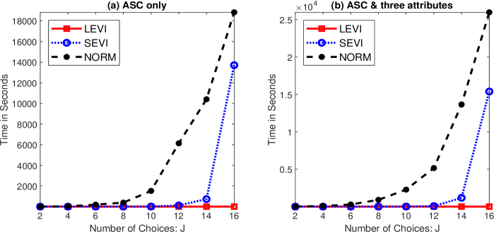
Figure 11: Comparison of computation times for the LEVI, SEVI, and NORM (standard MNP) models when $V_{ij}=Z_{i}\beta_{zj}$ or $V_{ij}=Z_{i}\beta_{zj}+X_{ij}\beta_{x}$

6 Some Extensions

6.1 Mixed LEVI-SEVI Model

One way to understand the random components in an RUM is to conceptualize them as capturing private signals exclusive to the individual agent making the choice, yet undisclosed to the econometrician (cf., Manski, (1977)). These signals may exhibit left or right skewness, varying across individuals. This variability suggests the possibility of two distinct groups of individuals: one characterized by the LEVI type and the other by the SEVI type. While the group membership of a specific individual remains unobservable, it is still useful to estimate the relative sizes of these two groups for the purpose of prediction and policy analysis.

Assume that individuals in the population have identical preference parameters but may differ in terms of random utility components. We postulate that with a probability of $\rho_{0},$ $\varepsilon_{ij}\thicksim iid$ $\mathrm{SEVI}$ over $j=1,\ldots,J$ and with a probability of $1-\rho_{0},$ $\varepsilon_{ij}\thicksim iid$ $\mathrm{LEVI}$ over $j=1,\ldots,J.$ In such a mixed LEVI-SEVI model, the probability of a randomly chosen individual, say individual $i,$ selecting alternative $j,$ given the vector of systematic utilities $v_{i},$ is

$$\Pr\left(Y_{i}=j|V_{i}=v_{i}\right)=\rho_{0}P^{\mathrm{SEVI}}\left(Y_{i}=j|V_{i}=v_{i}\right)+\left(1-\rho_{0}\right)P^{\mathrm{LEVI}}\left(Y_{i}=j|V_{i}=v_{i}\right).$$

Here, $\rho_{0}$ and $\left(1-\rho_{0}\right)$ can also be interpreted as the proportions of individuals belonging to the SEVI and LEVI types, respectively, in the population of interest.

This new latent class mixed LEVI-SEVI model (mixed LS model hereafter) differs from a usual latent class logit model where the classes have different preference parameters but the same random component. In the mixed LS model, identical preference parameters are assumed, but different random components are considered. Hence, it can be regarded as a mirror image of the usual latent class logit model.

While the identification, estimation, and inference of the mixed LS model warrant rigorous theoretical analysis, we present some simulation evidence suggesting that the key mixing parameter $\rho_{0}$ can be reliably estimated. We consider a parametrization of the systematic utilities as before where $X_{ij,\ell}\thicksim iidN(0,\pi^{2}\omega_{j}^{2}/36)$ for $\ell=1,2,3$ and $\beta_{0}=\left(1,2,1\right)^{\prime}$. We let the sample size be 5000 and consider $J=3,5,7,9.$ We estimate the model by MLE. Figure 12 presents a standard boxplot of the MLEs over 1000 simulation replications against the true value $\rho_{0}=0,0.1,0.2,\ldots,1.$ The diamond and bar markers inside each box indicate, respectively, the average and median of the MLEs for a given true value $\rho_{0},$ and the 45-degree line represents the true target line. Both the average and the median of the estimates are fairly close to the true value. The interquartile range (the difference between the 75th percentile and the 25th percentile) indicates some uncertainty in the estimator, particularly when $J$ is smaller, but this uncertainty diminishes as $J$ increases. Figures not reported here (see, for example, Figure S.8) show that the preference parameters can also be reliably estimated. Overall, our simulation results suggest that, with a reasonably large sample size, we can extract useful information on the mixing parameter and preference parameters. Consequently, a mixed LS model is an interesting alternative in empirical applications, especially given that it includes a SEVI model $(\rho_{0}=1)$ and a LEVI model $(\rho_{0}=0)$ as special cases. A natural extension is to specify the mixing parameter as a function of observable covariates that may influence whether an agent’s random component is LEVI or SEVI.

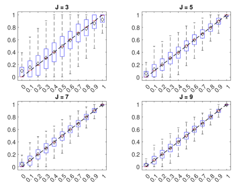
Figure 12: Boxplot of $\hat{\rho}$ for each true value $\rho_{0}=0,0.1,\ldots,1$ with sample size $5000$ and $J=3,5,7,9$

It is interesting to see how the QMLE under the usual conditional logit behaves when the true DGP is a mixed LS model. Figure 13 plots the average of $\hat{\beta}_{\mathrm{LEVI}}$ across the simulation replications against the true value of $\rho_{0}.$ When $\rho_{0}=0,$ the LEVI model is correctly specified, $\hat{\beta}_{\mathrm{LEVI}}$ is close to the true value $\beta_{0}$ in an average sense. When $\rho_{0}$ increases, signaling a higher misspecification of the LEVI model, the bias of $\hat{\beta}_{\mathrm{LEVI}}$ increases. For a given $\rho_{0}>0,$ the bias of $\hat{\beta}_{\mathrm{LEVI}}$ is larger when there are more alternatives. When $\rho_{0}=1,$ the DGP reduces to a SEVI model, and the figure aligns with the simulation results reported earlier.

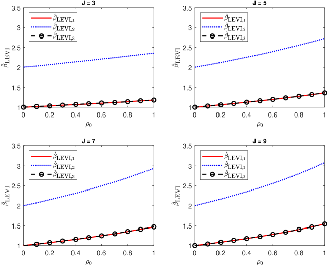
Figure 13: Plot of the average of $\hat{\beta}_{\mathrm{LEVI}}$ against $\rho_{0}$ with sample size 5000 and $J=3,5,7,9$

Finally, we evaluate the performance of a conventional mixed logit model when applied to data generated by a mixed LS model where $X_{ij,\ell}\thicksim iidN(0,\pi^{2}\omega_{j}^{2}/36)$ for $\ell=1,2,3$ and $\beta_{0}=\left(1,2,1\right)^{\prime}$. We let $\rho_{0}=0,0.25,0.50,0.75,$ and $1$ in the mixed LS model. We consider a large sample size of 50,000 and generate only one sample. Our experiment can be regarded as a large sample experiment. The preference parameters in the proposed mixed logit model are assumed to follow independent normal distributions. More specifically, $U_{ij}=X_{ij,1}\beta_{i,1}+X_{ij,2}\beta_{i,2}+X_{ij,3}\beta_{i,3}+\varepsilon_{ij}$ where $\varepsilon_{ij}$ is iid LEVI and $\beta_{i}:=\left(\beta_{i,1},\beta_{i,2},\beta_{i,3}\right)^{\prime}\thicksim\mathrm{iidN}(\beta,\mathrm{diag}\left(\sigma_{1}^{2},\sigma_{2}^{2},\sigma_{3}^{3}\right)).$ We refer to $\beta$ as the mean parameter and $\sigma=(\sigma_{1},\sigma_{2},\sigma_{3})^{\prime}$ as the standard deviation parameter. After fitting this mixed logit to the data generated by the mixed LS model, we consider three types of tests. First, we test whether $\beta=\beta_{0}$ using a standard Wald test. Second, we use the likelihood-ratio (LR) test for testing the null hypothesis of a logit model with fixed taste parameters (i.e., $\sigma^{2}=0)$ against the mixed logit. Finally, we use a generalized Hausman–McFadden (HM) test (Hahn et al., (2020)) for testing the null hypothesis that the mixed logit model is correctly specified. As in Hausman and McFadden, (1984), we first estimate the mixed logit model using the full sample and the subsample obtained by excluding individuals who chose the last alternative. We then compare these two estimates using a chi-square test. The comparison for the generalized HM test can be based on either the mean parameters or both the mean and standard deviation parameters. The generalized HM test targets the IIA property of mixed logit models at the individual level, and can be regarded as an IIA-oriented specification test that assesses whether the random utility components are iid LEVI. We set the nominal level for all three tests at 5%.

We provide a brief discussion of the simulation results. First, for all $J$ values $(3,5,7,9)$ considered, the mean parameter estimator has a positive bias, and the bias increases as $\rho_{0}$ or $J$ increases. The Wald test rejects the null that the mean parameter is equal to $\beta_{0}$ when $\rho_{0}\geq 0.25$ for all $J$ values. This suggests that a mixed logit model fitted to the data generated by a mixed LS model can not reliably recover the mean preference parameters.

Second, the LR test fails to reject the null hypothesis of fixed taste parameters when either $\rho_{0}$ smaller than or equal to $0.5$ or when $J$ $\leq 5$. In these cases, the mixed logit does not significantly improve the fit relative to the fixed-parameter logit model, with the standard deviation parameters typically being insignificant. This suggests that the normally distributed taste parameters are not able to pick up the SEVI random component. On the other hand, the LR test rejects the null of fixed taste parameters when both $\rho_{0}$ and $J$ are large. In these cases, a large $\rho_{0}$ $(\rho_{0}\geq 0.75)$ and a large $J$ $\left(J\geq 7\right)$ prompt the LR test to mistake heterogeneity in the random utility components for heterogeneity in the taste parameters. While the LR test tends to be conservative as the variance parameters are on the boundary under the null, our simulation results highlight that its use can lead to the incorrect conclusion of taste heterogeneity when the taste parameters are the same for all individuals.

Finally, the generalized HM test based on the mean parameters rejects the null of iid LEVI random utility components when $\rho_{0}\geq 0.75$ and $J\geq 7$. On the other hand, the generalized HM test based on both the mean and standard deviation parameters rejects the null of iid LEVI random utility components for almost all $\rho_{0}$ and $J$ values considered.

These findings generally remain valid with minimal exceptions when the random preference parameters follow a normal distribution with an unrestricted variance matrix.

In summary, a mixed logit model with correlated or uncorrelated preference parameters will not be far off when $\rho_{0}$ is small, but it may yield misleading preference estimates even with a moderately large $\rho_{0}$. Notably, the mixed logit model can mistake heterogeneity in the random utility components for taste heterogeneity, particularly in situations with a large $\rho_{0}$ and a large $J$. Consequently, the mixed logit model is not a reliable substitute for the mixed LS model.

6.2 Cost Minimizing Choice

In some empirical applications, economic agents may choose one alternative from a set of alternatives to minimize a specific objective function, such as cost, regret, disutility, or loss, rather than maximizing it. For instance, in the study by Fowlie, (2010), which we will examine in the next section, plant managers choose an environmental compliance strategy in order to minimize their overall cost.

To model the minimization behavior, we assume that there is a latent function $C_{ij}$ that encompasses an observable component $D_{ij}\left(\beta_{0}\right)$ and an unobservable component $\varepsilon_{ij},$ so that

$$C_{ij}\left(\beta_{0}\right)=D_{ij}\left(\beta_{0}\right)+\varepsilon_{ij}\text{ for }j=1,\ldots,J\text{ }$$

where $C_{ij}\left(\beta_{0}\right)$ is the ‘cost’ that individual $i$ incurs from choosing alternative $j.$ Individuals then make a choice that results in the smallest $C$ value. More specifically, the observed choice of individual $i$, denoted by $Y_{i},$ equals

$$Y_{i}=\arg\min_{j=1,\ldots,J}C_{ij}\left(\beta_{0}\right).$$

Assuming that $\left\{D_{ij}\left(\beta_{0}\right)\right\}_{j=1}^{J}$ and $\left\{\varepsilon_{ij}\right\}_{j=1}^{J}$ are independent of each other, we consider two cases: either $\varepsilon_{ij}\thicksim^{iid}\mathrm{LEVI}$ or $\varepsilon_{ij}\thicksim^{iid}\mathrm{SEVI.}$ Let $D_{i}\left(\beta_{0}\right)=(D_{i1}\left(\beta_{0}\right),\ldots,D_{iJ}\left(\beta_{0}\right))^{\prime}\in\mathbb{R}^{J}$ and $d_{i}\in\mathbb{R}^{J}$ be a point in the support of $D_{i}\left(\beta_{0}\right).$ In the former case, we have

$$\Pr(Y_{i} =j|D_{i}\left(\beta_{0}\right)=d_{i},\varepsilon_{i,m}\overset{iid}{\thicksim}\mathrm{LEVI})$$

$$=\Pr\left(d_{ij}+\varepsilon_{i,j}\leq d_{ik}+\varepsilon_{i,k}\text{, }k\in\mathcal{J},\varepsilon_{i,m}\overset{iid}{\thicksim}\mathrm{LEVI}\right)$$

$$=\Pr\left(-d_{ij}-\varepsilon_{i,j}\geq d_{ik}-\varepsilon_{i,k},\text{ }k\in\mathcal{J},\text{ }\varepsilon_{i,m}\overset{iid}{\thicksim}\mathrm{LEVI}\right)$$

$$=\Pr\left(-d_{ij}+\varepsilon_{i,j}\geq-d_{ik}+\varepsilon_{i,k},\text{ }k\in\mathcal{J},\varepsilon_{i,m}\overset{iid}{\thicksim}\mathrm{SEVI}\right)$$

$$=P^{\mathrm{SEVI}}\left(Y_{i}=j|-d_{i}\right),$$

where $P^{\mathrm{SEVI}}\left(Y_{i}=j|-d_{i}\right)$ is defined in (6). In the latter case, we have, using the same argument,

$$\Pr(Y_{i}=j|D_{i}\left(\beta_{0}\right)=d_{i},\varepsilon_{i,m}\overset{iid}{\thicksim}\mathrm{SEVI})=P^{\mathrm{LEVI}}\left(Y_{i}=j|-d_{i}\right),$$

where $P^{\mathrm{LEVI}}\left(Y_{i}=j|-d_{i}\right)$ is defined in (7). So, for discrete choice problems aiming at minimizing an objective function, when $\varepsilon_{i,j}\overset{iid}{\thicksim}\mathrm{LEVI,}$ the choice probability takes the form of (6). In contrast, when $\varepsilon_{i,j}\overset{iid}{\thicksim}\mathrm{SEVI,}$ the choice probability takes the usual logit form.

Note that there is a sign change. It is $-d_{i}$ rather than $d_{i}$ itself that enters the expression of the choice probability derived under utility maximization. If we parameterize $D_{ij}\left(\beta_{0}\right)=X_{ij}\beta_{0}$ for some covariate $X_{ij}$ and run a conditional logit using $X_{ij}$ as the covariate in a statistical package, then we are assuming that $\varepsilon_{i,j}\overset{iid}{\thicksim}\mathrm{SEVI}$, and what the package returns is an estimate of $-\beta_{0}.$ To correct this, we can flip the sign of the estimate or use the flipped covariate $-X_{ij}$ as the covariate.

If we deem that $\varepsilon_{i,j}\overset{iid}{\thicksim}\mathrm{LEVI}$ is more plausible, then the choice probability formula in (6) has to be used, and the approach proposed in this paper can be easily applied.

Irrespective of whether we are dealing with a minimization or maximization choice problem, we call a model with SEVI errors a SEVI model and a model with LEVI errors a LEVI model. In the case of maximization problems, estimating a LEVI model is more straightforward, while for minimization problems, a SEVI model is easier to estimate.

7 Empirical Applications

In this section, we examine four commonly used datasets from well-cited textbooks and papers, all of which have been included in the mlogit package in R (cf., Croissant, (2020)). For each dataset, we apply three distinct models: the LEVI model, the SEVI model, and the NORM model (i.e., a multinomial probit model with iid $N\left(0,\pi^{2}/6\right)$ errors). The variances of random utility components of all three models are the same and equal to $\pi^{2}/6.$ The sole difference among these three models lies in the shape of the distributions of the random utility components.

The four datasets we analyze are:

1. Fishing mode choice: the dataset comes from (Herriges and Kling, (1999)), which has been analyzed in several textbooks, including Cameron and Trivedi, (2005), Cameron and Trivedi, 2022a , and Cameron and Trivedi, 2022b .

2. Stated preference vehicle choice: the dataset originates from Brownstone et al., (1996) and is subsequently used in Brownstone and Train, (1998) and McFadden and Train, (2000).

3. Choice of brand for saltine crackers: the dataset originates from Paap and Franses, (2000), and a subset of the data was analyzed in Jain et al., (1994).

4. Choice of NO_x emissions compliance strategies: the dataset comes from Fowlie, (2010).

Table 3 presents the computation times and log-likelihood performances of the three models. In all cases, the computational time represents the seconds spent by our MATLAB program on finding the MLE/QMLE. Although there may be slight fluctuations in the reported computation times due to concurrent background processes, they serve as a reliable indicator of the time needed for estimating each model. We will revisit this table when we discuss each application.

Table 3: Performances of LEVI, SEVI, and NORM on several data sets

Data Set	${\small n}$	${\small J}$	${\small L}$	Computation time			Log-likelihood			Likelihood
				LEVI	SEVI	NORM	LEVI	SEVI	NORM	Ranking
Fishing	1182	4	8	0.35	0.58	370	-1215.14	-1213.21	-1218.93	S $>$ L $>$ N
Vehicles	4654	6	21	3.57	14.00	2232	-7394.62	-7388.75	-7389.50	S $>$ N $>$ L
Crackers	3289	4	6	0.31	0.55	157	-3347.61	-3347.13	-3344.51	N $>$ S $>$ L
NOx: dereg	227	15	6	135.00	0.02	791	-345.35	-339.07	-343.21	S $>$ N $>$ L
NOx: public	113	15	6	78.00	0.01	2357	-86.30	-78.46	-82.38	S $>$ N $>$ L
NOx: reg	292	15	6	279.00	0.01	4600	-364.99	-359.74	-365.96	S $>$ L $>$ N
(i) ${\small n}$  is the # of choice situations, ${\small J}$ is the (max) # of alternatives, and ${\small L}$ is the total # of covariates.
(ii) “NOx: dereg” is the subsample of deregulated plants; “NOx: public” is the subsample of public plants,
and “NOx: reg” is the subsample of “regulated” plants.
(iii) All computation times are measured in seconds.
(iv) In the likelihood ranking, S, L, and N are short for SEVI, LEVI, and NORM, respectively.

7.1 Application: Choice of Fishing Mode

For the fishing mode application, we model an individual’s choice of fishing modes among four mutually exclusive alternatives: beach $(j=1)$, pier $\left(j=2\right)$, private boat $(j=3)$, and charter boat $(j=4)$. We assume that the latent utility is given by

$$U_{ij} =X_{1j}\beta_{x1}+X_{2j}\beta_{x2}+D2_{j}\times\beta_{d2}+D3_{j}\times\beta_{d3}+D4_{j}\times\beta_{d4}$$

$$+\left(Z_{i}\cdot D2_{j}\right)\times\beta_{z2}+\left(Z_{i}\cdot D3_{j}\right)\times\beta_{z3}+\left(Z_{i}\cdot D4_{j}\right)\times\beta_{z4}+\varepsilon_{ij},$$

where $X_{1j}$ and $X_{2j}$ are the price and catch rate of alternative $j$, $D2_{j},D3_{j}$, and $D4_{j}$ are the dummy variables for alternatives 2, 3, and 4, respectively, and $Z_{i}$ is the income of individual $i.$ For this application, the LEVI and SEVI models yield similar parameter estimates and likelihood function values. The correlation coefficient between the in-sample predicted choice probabilities for the two models is 0.998, indicating a nearly perfect positive correlation between them. Both models can be estimated with minimal computational cost with the optimization algorithm completing in less than a minute. Nevertheless, the SEVI model has a higher log-likelihood than the LEVI model. In contrast, the multinomial probit incurs significantly higher computational costs and yields a lower log-likelihood compared to both the LEVI and SEVI models.

Figure 14 plots the difference between the predicted choice probabilities (i.e., $P^{\mathrm{SEVI}}(\hat{\beta}_{\mathrm{SEVI}})-P^{\mathrm{LEVI}}(\hat{\beta}_{\mathrm{LEVI}})$ or $P^{\mathrm{NORM}}(\hat{\beta}_{\mathrm{NORM}})-P^{\mathrm{LEVI}}(\hat{\beta}_{\mathrm{LEVI}}))$ against $P^{\mathrm{LEVI}}(\hat{\beta}_{\mathrm{LEVI}}).$ While all three predicted choice probabilities are very highly correlated, the figure illustrates some subtle distinctions. Specifically, as $P^{\mathrm{LEVI}}(\hat{\beta}_{\mathrm{LEVI}})$ increases, the variabilities of $P^{\mathrm{SEVI}}(\hat{\beta}_{\mathrm{SEVI}})-P^{\mathrm{LEVI}}(\hat{\beta}_{\mathrm{LEVI}})$ and $P^{\mathrm{NORM}}(\hat{\beta}_{\mathrm{NORM}})-P^{\mathrm{LEVI}}(\hat{\beta}_{\mathrm{LEVI}})$ also increase, indicating that the three models tend to align closely when the choice probabilities are low but exhibit discrepancies otherwise.

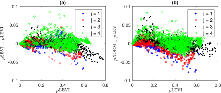
Figure 14: Plot of the difference of the predicted choice probabilities against the LEVI predicted probability in the fishing mode choice application

To illustrate the difference between the SEVI and LEVI models using the fishing choice data, we calculate the choice probabilities $P^{\mathrm{LEVI}}(\hat{\beta}_{\mathrm{LEVI}})$ and $P^{\mathrm{SEVI}}(\hat{\beta}_{\mathrm{LEVI}})$ using the same parameter value $\hat{\beta}_{\mathrm{LEVI}}.$ Figure S.9 plots $P^{\mathrm{SEVI}}(\hat{\beta}_{\mathrm{LEVI}})$ against $P^{\mathrm{LEVI}}(\hat{\beta}_{\mathrm{LEVI}})$. We find that when $P^{\mathrm{LEVI}}(\hat{\beta}_{\mathrm{LEVI}})$ is small, $P^{\mathrm{SEVI}}(\hat{\beta}_{\mathrm{LEVI}})$ tends to be smaller than $P^{\mathrm{LEVI}}(\hat{\beta}_{\mathrm{LEVI}})$, and when $P^{\mathrm{LEVI}}(\hat{\beta}_{\mathrm{LEVI}})$ is large, $P^{\mathrm{SEVI}}(\hat{\beta}_{\mathrm{LEVI}})$ tends to be larger than $P^{\mathrm{LEVI}}(\hat{\beta}_{\mathrm{LEVI}})$. This observation aligns with the previously reported simulation results, as seen in Figure 5, for example.

7.2 Application: Stated Preferences for Vehicle Choice

For the stated preference vehicle data, each individual was presented with 6 hypothetical vehicles fueled by methanol, compressed natural gas, electricity or regular gas. These vehicles have various attributes, such as fuel type, price, cost per mile, mileage range between refuelings/rechargings, vehicle type (SUV, sports car, station wagon, truck, van, regular car), pollution level, and speed, among others. We employ the same set of 21 covariates as in McFadden and Train, (2000) (Table 1), some of which are the products of vehicle attributes and individual characteristics, such as household size greater than 2 or not, college education or not, and a daily commute of less than 5 miles or not.

As shown in Table 3, in terms of the log-likelihood achieved, the LEVI model performs worse than the SEVI model and the NORM model.

Figures 15 (a) and (b) plot the difference in the predicted probabilities (i.e., $P^{\mathrm{SEVI}}(\hat{\beta}_{\mathrm{SEVI}})-P^{\mathrm{LEVI}}(\hat{\beta}_{\mathrm{LEVI}})$ or $P^{\mathrm{NORM}}(\hat{\beta}_{\mathrm{NORM}})-P^{\mathrm{LEVI}}(\hat{\beta}_{\mathrm{LEVI}})$ against the LEVI predicted probability (i.e., $P^{\mathrm{LEVI}}(\hat{\beta}_{\mathrm{LEVI}})$. There are some intriguing patterns. Figure 15(a) shows that $P^{\mathrm{SEVI}}(\hat{\beta}_{\mathrm{SEVI}})$ tends to be higher than $P^{\mathrm{LEVI}}(\hat{\beta}_{\mathrm{LEVI}})$ when the latter is low and tends to be lower than $P^{\mathrm{LEVI}}(\hat{\beta}_{\mathrm{LEVI}})$ when the latter is high.

Note that the difference $P^{\mathrm{SEVI}}(\hat{\beta}_{\mathrm{SEVI}})-P^{\mathrm{LEVI}}(\hat{\beta}_{\mathrm{LEVI}})$ can be decomposed as

$$P^{\mathrm{SEVI}}(\hat{\beta}_{\mathrm{SEVI}})-P^{\mathrm{LEVI}}(\hat{\beta}_{\mathrm{LEVI}})=\text{ }\underset{\text{I}}{\underbrace{P^{\mathrm{SEVI}}(\hat{\beta}_{\mathrm{SEVI}})-P^{\mathrm{SEVI}}(\hat{\beta}_{\mathrm{LEVI}})}}+\underset{\text{II}}{\underbrace{P^{\mathrm{SEVI}}(\hat{\beta}_{\mathrm{LEVI}})-P^{\mathrm{LEVI}}(\hat{\beta}_{\mathrm{LEVI}})}}.$$

The first part (I) above is due to the difference in the parameter estimates used ($\hat{\beta}_{\mathrm{SEVI}}$ vs. $\hat{\beta}_{\mathrm{LEVI}})$, and the second part (II) above is due to the difference in the predictive models used (SEVI vs. LEVI). According to an unreported figure, the second part exhibits the same pattern as in Figure 5. So the pattern in Figure 15(a) emerges because the effect of the first part dominates that of the second part. Figure 15(b) shows a similar pattern, although $P^{\mathrm{NORM}}(\hat{\beta}_{\mathrm{NORM}})-P^{\mathrm{LEVI}}(\hat{\beta}_{\mathrm{LEVI}})$ appears to be less variable than $P^{\mathrm{SEVI}}(\hat{\beta}_{\mathrm{SEVI}})-P^{\mathrm{LEVI}}(\hat{\beta}_{\mathrm{LEVI}}).$

Figures 15 (c) and (d) are similar to Figures 15 (a) and (b) but use $P^{\mathrm{NORM}}(\hat{\beta}_{\mathrm{NORM}})$ as the benchmark. According to these two figures, $P^{\mathrm{SEVI}}(\hat{\beta}_{\mathrm{SEVI}})-P^{\mathrm{NORM}}(\hat{\beta}_{\mathrm{NORM}})$ and $P^{\mathrm{LEVI}}(\hat{\beta}_{\mathrm{LEVI}})-P^{\mathrm{NORM}}(\hat{\beta}_{\mathrm{NORM}})$ display opposite patterns. On one hand, $P^{\mathrm{SEVI}}(\hat{\beta}_{\mathrm{SEVI}})$ tends to be higher than $P^{\mathrm{NORM}}(\hat{\beta}_{\mathrm{NORM}})$ when the latter is low and tends to be lower than $P^{\mathrm{NORM}}(\hat{\beta}_{\mathrm{NORM}})$ when the latter is high. On the other hand, $P^{\mathrm{LEVI}}(\hat{\beta}_{\mathrm{LEVI}})$ tends to be lower than $P^{\mathrm{NORM}}(\hat{\beta}_{\mathrm{NORM}})$ when the latter is low and tends to be higher than $P^{\mathrm{NORM}}(\hat{\beta}_{\mathrm{NORM}})$ when the latter is high. Clearly, the decision to employ SEVI, NORM, and LEVI random components can have a significant effect on the predicted choice probabilities.

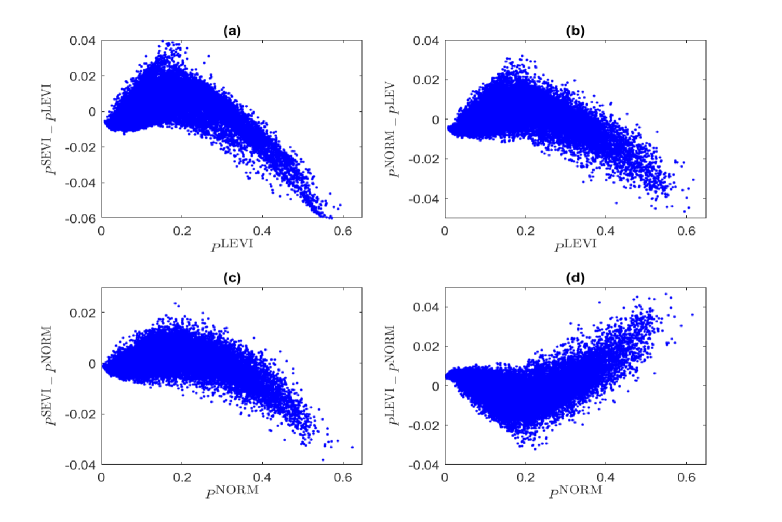
Figure 15: Plot of the difference of the predicted choice probabilities against the LEVI or NORM predicted probability in the vehicle choice application

We also report the point estimates of the parameters under the LEVI and SEVI model, along with their 95% confidence intervals. See Figure S.10 in the supplementary appendix. While the CI’s for 14 parameters clearly overlap, those for $6$ parameters either do not overlap or barely overlap. In practical terms, this divergence suggests that the two models may lead to different conclusions regarding the impact of certain attributes on vehicle choices. Specifically, attributes such as mileage range between refuelings/rechargings, cost per mile, and vehicle types exhibit different effects in the LEVI and SEVI models. Compared to the LEVI model, the SEVI model suggests that the mileage range between refuelings/rechargings and the vehicle’s classification as an SUV (rather than a regular car) are less influential factors. On the other hand, the cost per mile and other vehicle types (rather than a regular car) appear to be more influential in the SEVI model.

7.3 Application: Choice of Saltine Crackers

The dataset on saltine cracker choices contains information on all purchases of crackers (3292) of 136 households, including the brand chosen from four alternative brands, prices of all four brands (Price), whether there was an in-store display of the brand (Display dummy) and/or whether the brand was featured in the store’s newspaper advertising (Feature dummy) at the time of purchase. The latent utility is specified as follows:

$$U_{ij} =\mathtt{Price}\text{ }\times\beta_{x1}+\mathtt{Display}\text{ }\times\beta_{x2}+\mathtt{Feature}\text{ }\times\beta_{x3}$$

$$+D2_{j}\times\beta_{d2}+D3_{j}\times\beta_{d3}+D4_{j}\times\beta_{d4}+\varepsilon_{ij},$$

where $j=1,2,3,4$ corresponding to the brands “Sunshine”, “Keebler”, “Nabisco”, “Private” (a private-label brand), respectively, and $D2,\,D3,$ and $D4$ are dummies for the latter three brands (the dummy for the first band has been omitted to achieve identification).

For this application, individuals made repeated purchase decisions. Choice situations belonging to the same individual are possibly correlated. To account for the correlation, we treat each individual as a cluster and employ cluster-robust standard errors. An unreported figure similar to Figure S.10 shows that the estimated coefficients on the three main covariates (Price, Display, and Feature) are similar across the LEVI and SEVI models. However, the alternative-specific coefficients on D2, D3, and D4 are different across these two models. As shown in Table 3, the SEVI model has a slightly higher log-likelihood compared to the LEVI model, although the difference is small.

As shown in Table 3, the NORM model has a higher log-likelihood than both the LEVI model and the SEVI model. This may indicate that the random utility component is symmetrically distributed so that a normal distribution, which is symmetric, might provide a more accurate characterization than the LEVI and SEVI distributions. Figure 16 plots the difference in the predicted choice probabilities using the NORM probability as the benchmark, highlighting distinct deviations between the SEVI and LEVI probabilities from the NORM probability.

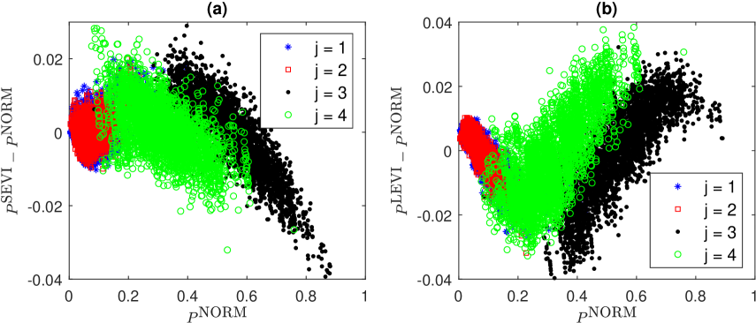
Figure 16: Plot of the difference of the predicted choice probabilities against the multinomial probit predicted probability in the cracker choice application

7.4 Application: Choice of a NO_x Emissions Reduction Technology

Managers of coal-fired electric power plants chose a NO_x emissions reduction technology in order to comply with a regional NO_x emissions trading program. The manager of a plant unit, say unit $i,$ chooses a compliance strategy from $J_{i}$ alternatives indexed by $j=1,\ldots,J_{i}$ to minimize the unobserved overall cost $C_{ij}.$ We assume that

$$C_{i,j}=X_{ij}\beta+\varepsilon_{i,j}$$

for $j=1,\ldots,J_{i}$ where $X_{ij}$ comprises observed factors that affect the cost and $\varepsilon_{i,j}$ captures unobserved cost shifters. We assume that these two components are independent of each other. The observed choice is indicated by $Y_{i}=\arg\min_{j=1}^{J_{i}}C_{i,j}$. The model is essentially the same as that outlined in Section 6.2 but there are two differences. First, the maximum number of options is 15 but not all options are available for each plant. To accommodate this, we simply assign an infinite systematic cost to any unavailable option, ensuring it is never selected. This may not be computationally efficient, but the number of options becomes the same for all choice situations. In addition, this method effectively provides us with an empirical example when the number of alternatives is quite large. Second, some plants have the same manager so there may be dependence in the unobserved costs across these plants. Following standard practice, we will not consider the dependence when constructing the likelihood function. That is, we will use a partial likelihood approach, but we account for the dependence in estimating the asymptotic variance by clustering the managers.

The compliance options have different capital costs (denoted by kcost_ij) and variable operating costs (denoted by vcost_ij). Each compliance option incorporates one or more of the following three technologies: post-combustion pollution control technology (indicated by the dummy post_j), combustion modification technology (indicated by the dummy cm_j), and low NO_x burners technology (indicated by the dummy lnb_j). Taking these into consideration, we follow Fowlie, (2010) and let $X_{ij}=$ (post${}_{j},$ cm${}_{j},$ lnb${}_{j},$ kcost${}_{ij},$ vcost${}_{ij},$ kage_ij) where kage = kcost $\times$ age and age is the age of a plant.

The plants are in one of the three regulatory environments: they are either “deregulated”, “public”, or “regulated”. The central question investigated by Fowlie, (2010) is whether and how regulatory environments influence a manager’s choice of compliance strategies. The question can be addressed by comparing the coefficient estimates across the subsamples of “deregulated”, “public”, or “regulated” plants.

We apply the LEVI, SEVI, and NORM models to each subsample and evaluate their performances. Table 3 shows that the SEVI model, which assumes that $\varepsilon_{i,j}\overset{iid}{\thicksim}\mathrm{SEVI}$, achieves the highest likelihood among the three models and for all three subsamples. We note that Fowlie, (2010) made this SEVI assumption implicitly, and in doing so, happened to use the model out of these three with the highest likelihood.

The parameter estimates and the clustered-robust standard errors are reported in Table 4. For each of the three models, the coefficients vary significantly across different regulatory environments. In particular, the coefficient on capital cost (kcost) based on the “deregulated” subsample is positive and statistically significant at the 1% level, but those based on the “public” subsample and the “regulated” subsample are negative, albeit not statistically significant. This implies that plant managers give more weight to capital cost if their plants are in a “deregulated” market rather than a “public” or “regularized” market. Our findings confirm the main result of Fowlie, (2010) and show that the result is robust to the LEVI specification of the random cost component.

	$\hat{\beta}_{\mathrm{LEVI}}$	se:$\hat{\beta}_{\mathrm{LEVI}}$	$\hat{\beta}_{\mathrm{SEVI}}$	se:$\hat{\beta}_{\mathrm{SEVI}}$	$\hat{\beta}_{\mathrm{NORM}}$	se:$\hat{\beta}_{\mathrm{NORM}}$
	Deregulated
post	1.502	0.106	0.862	0.056	1.245	0.177
cm	1.538	0.120	0.859	0.068	1.250	0.155
lnb	1.551	0.121	0.784	0.064	1.193	0.175
vcost	0.188	0.045	0.112	0.030	0.145	0.041
kcost	0.060	0.020	0.036	0.012	0.050	0.018
kage	0.037	0.008	0.028	0.004	0.037	0.010
	Public
post	5.706	1.050	3.890	0.601	4.927	0.824
cm	4.433	0.442	2.685	0.193	3.589	0.384
lnb	3.964	0.307	2.532	0.201	3.323	0.463
vcost	1.564	0.604	0.840	0.293	1.177	0.270
kcost	-0.039	0.255	-0.100	0.118	-0.086	0.088
kage	0.080	0.046	0.024	0.027	0.049	0.038
	Regulated
post	2.665	0.142	1.680	0.070	2.302	0.213
cm	1.911	0.103	1.250	0.058	1.686	0.151
lnb	2.208	0.111	1.377	0.057	1.884	0.180
vcost	0.278	0.045	0.171	0.028	0.196	0.047
kcost	-0.008	0.023	-0.005	0.013	-0.023	0.022
kage	0.023	0.005	0.014	0.003	0.010	0.008

Table 4: Parameter estimates and standard errors: environmental compliance choices.

Note that for the same subsample, the coefficients in the LEVI and SEVI models may be directly compared. For the “deregulated” subsample, each element of $\hat{\beta}_{\mathrm{LEVI}}$ is larger than the corresponding element of $\hat{\beta}_{\mathrm{SEVI}}$ by more than 50%. For the “public” or “regularized” subsamples, the coefficients on post, cm,lnb, vcost, and kage in the LEVI model are larger than those in the SEVI model by at least 50%. This indicates the significance of the model choice on the parameter estimates with consequential implications on policy recommendations.

7.5 Further Remarks on the Empirical Applications

We conclude the empirical application by making some further comments on the rankings of the three models according to their likelihood values and computation times.

First, in terms of likelihood values, the SEVI model outperforms the LEVI model across all considered applications. With the exception of the cracker brand application, the SEVI model achieves the highest likelihood value among all three models. Notably, in the application of choosing an environmental compliance strategy, the SEVI model yields a choice probability in the conventional logit form, as the focus is on minimizing, rather than maximizing, an objective function. Overall, regardless of whether an agent aims to minimize or maximize an objective function, the SEVI distribution proves to be an important contender for characterizing the random components in a discrete choice model.

Second, for all applications, the computation time is shortest when the choice probabilities take the standard LEVI-based logit form. When the number of alternatives, $J,$ is not larger than 6, the computation time for the model with the extended choice probability formula, as given in (6), is only two to four times as large as that for the computationally simplest model and is much lower than that for the multinomial probit model. When $J=15,$ the computation time for the model with the extended choice probability formula remains significantly lower than that of the multinomial probit model, although the competitive advantage is not as pronounced as when $J$ is smaller.

8 Conclusions and Further Research Directions

In a random utility model, individuals make choices among a set of alternatives based on their utilities. These utilities are typically assumed to consist of a systematic component, representing aspects of the choice alternatives that are observable to the analyst, and a random component, capturing factors that may be known only to the decision makers. Typically, the random components are assumed to follow the right-skewed largest extreme value Type I (LEVI) distribution, leading to the standard multinomial and conditional logit models and their generalizations. In this paper, we ask the question: what if the random component followed, instead, the left-skewed smallest extreme value type I (SEVI) distribution? A priori, there is no reason to support choosing LEVI over SEVI as correct beyond one’s prior belief with respect to the skewness of the RUM’s random component.

We show that the SEVI-based choice probabilities still have closed-form expressions, although they are not as simple as those in the standard logit models. We use the MLE to estimate the RUM when the random component follows the smallest extreme value type I distribution and show that standard asymptotic theory, including the asymptotic normality of the MLE, works well in finite samples. We provide an approach based on Gosper’s hack to efficiently compute the choice probabilities and the MLE for the SEVI model.

If one incorrectly assumes the random component follows LEVI when SEVI is appropriate and applies the standard logit, the resulting QMLE can have a large bias arising from misspecification. A distinctive feature of this setup is that this bias increases with the size of the choice set. The bias also has important effects on estimating standard economic quantities such as average partial effects and elasticities, as well as predicting the out-of-sample choice probabilities. The LEVI and SEVI models exhibit distinctly different patterns of substitution, with the former conforming to IIA and the latter exhibiting a particular way of weighting outcomes from all subsets comprised of two or more alternatives.

In an important way, the distinction between the LEVI and SEVI models is more striking than the long-standing comparisons of a LEVI model versus a multinomial probit model. The latter comparisons have focused on the theoretical convenience of a multinomial probit to allow for correlated error components. In a SEVI model, the error components exhibit no correlation, yet the patterns of substitutions are considerably more intricate compared to a LEVI model. In particular, IIA does not hold in a SEVI model with more than two alternatives, even though the random utilities are iid and still follow an extreme value distribution. Furthermore, for the same estimate of an agent’s preference parameters, the predicted probabilities based on the LEVI and SEVI models are typically different in predictable and economically meaningful ways.

The fundamental question when choosing between the LEVI and SEVI models revolves around whether the random utility is more likely to be positive, as is the case with LEVI, or negative, as is the case with SEVI. This is crucial in a choice context because increasing the magnitude of the random utility is typically of little or no consequence in a choice model since the “scale” is not separately identified as long as all of the random components come from the same iid distribution. This is not true in general for the skewness of the distribution when there are more than two alternatives. A key takeaway from this paper is that we should pay more attention to the skewness of a distribution when it is used to model the random components in a discrete choice model. From a practical point of view, we may use past empirical evidence, if any, to decide whether the stochastic utility is likely to be positively or negatively skewed. If we do not have such guidance, we may use the model that has a higher likelihood function in an AIC/BIC sense or employ Vuong’s test to decide which model better fits the data at hand.

There are many possible extensions of our work. Below, we discuss a few possibilities within the utility maximization framework, keeping in mind that all discussions apply to discrete decision-making problems aimed at minimizing an objective function.

First, the LEVI-based conditional and multinomial logit models have been extended in a number of ways, often in an effort to allow a more flexible substitution pattern than the IIA. These extensions are generally amenable to using the SEVI-based conditional logit core in place of the current LEVI one. Consider, for example, the simplest version of the latent class conditional logit model, where there are two classes with each characterized by a standard conditional logit model with potentially different vectors of preference parameters and a mixing fraction. The standard conditional logit model can be swapped out here for its SEVI-based counterpart and a variant of the Vuong test described earlier can be used to help distinguish between them. As discussed in 6.1, another variant of the latent class framework would be to allow one of the classes to be based on a LEVI-conditional logit model and the other to be characterized by a SEVI-conditional logit model with the same preference parameters across the two classes. Still, a different version would extend the scale heterogeneity LEVI model to the SEVI context by allowing for two SEVI conditional logit models with common preference parameters but different error component variances, influenced by exogenous factors. These factors might include sources of the samples, such as whether the data pertains to observed decisions or stated preference surveys, and whether the data comes from different regulatory environments, as exemplified in one of our empirical applications. Obviously, these can all be extended to more than two latent classes and combined in various ways, such as LEVI and SEVI classes with different preference parameters. One could envision an EM algorithm that alternates between fixing preference parameters and estimating the mixing proportion, and vice versa.

Second, while latent class LEVI variants are quite popular in marketing because of their “segmentation” interpretation and the use of covariates to predict segment memberships, random parameter variants of conditional logit models have attracted more attention from economists who find the notion of a continuum of preference parameters in the population appealing. Nothing in this appeal is tied to the LEVI versus SEVI distinction in the nature of the random utility component. As such, there is no conceptual issue involved in swapping the LEVI-core for a SEVI-core against which the random parameter distributions will be defined.

Third, there are various other flavors of logit models used by economists. The nested logit explicitly allows a correlation between different subsets of alternatives that are uncorrelated within a nest. Exploring the properties of the SEVI analogue would be of interest, given the quite different patterns of substitution within a nest. The generalized multinomial logit’s gamma parameter determines how the random component of the mixed logit interacts with the scale parameter (Fiebig et al., (2010)). It is unclear how this tradeoff is influenced by a SEVI or LEVI core. Another interesting question is how the cut-off points and parameter estimates are influenced in an ordered logit model when switching its foundation from LEVI to SEVI error components. As discussed in Section 3.3, the SEVI analogue of the LEVI-type model for completely rank-ordered can be developed, but the exact details warrant further studies.

Fourth, while the conditional logit and its generalizations dominate empirical economic work, the statistically equivalent multinomial/polychotomous logit models are heavily used in biomedical sciences and in other social sciences. The same issues involving LEVI and SEVI arise in these models. For instance, in a political election, such as an open party primary for a legislative seat, beyond the set of attributes available in the official voter’s pamphlet, is the voter likely to learn information that, on average, improves their perception of the candidate’s quality/suitability (LEVI) or decreases (SEVI)? Predominance of negative advertising suggests SEVI might be more likely in some contexts.

Fifth, multinomial logistic regression is one of the basic tools taught to budding data scientists. Its kernel forms the basis of other more complex procedures, including some flavors of neural networks. Further, multinomial classification problems are often addressed using the multinomial logit objective function coupled with variable section procedures like LASSO when there are a large number of potential predictors. There are SEVI variants of all of these that could be explored.

Finally, along a very different path, cleverly designed discrete choice experiments can help shed light on whether all/most agents have random utility components that are left-skewed, symmetric, or right-skewed. There are a number of interesting questions along this avenue. For example, does the skewness of the random component vary with deeper aspects of preferences, such as risk aversion from economics or openness to new experiences from psychology (Jagelka, (2024) and Jiang et al., (2024))? Does the skewness vary with observable demographic characteristics like age and gender, or is it largely a function of educational attainment? Does it vary by potentially quantifiable differences in how agents obtain information? Does it also vary with specific aspects of the larger context in which the choice opportunity is embedded? Does observing repeated choices by the same agent in similar contexts over time offer more power to identifying an agent’s skewness type, or is it possible that agents shift from one type when the choice set is novel to another type when the choice opportunity is relatively routine? There are a number of comparisons of LEVI versus SEVI in different contexts that should be of broad interest: revealed versus stated preference data, in-store versus online purchases, private versus public goods, eliciting the best versus the worst alternative in a set, choices involving different forms of uncertainty, and choices involving gains versus losses. Our work provides tools to examine these issues.

9 Appendix of Proofs

Proof of Theorem 1. A direct algebraic proof is given in the supplementary appendix (see Section S.A). Here, we prove the result using the inclusion-exclusion principle. For each $k\in\mathcal{J}_{-j}:=\left\{1,\ldots,J\right\}\backslash\left\{j\right\}$, define the event

$$\mathcal{E}_{k,j}:v_{ij}+\varepsilon_{ij}\geq v_{ik}+\varepsilon_{ik},$$

where $\varepsilon_{ij}\thicksim iid$ $\mathrm{SEVI}$ over $j\in\mathcal{J}$. Equivalently, we define the event $\mathcal{E}_{k,j}$ as

$$\mathcal{E}_{k,j}:-v_{ij}+\tilde{\varepsilon}_{ij}\leq-v_{ik}+\tilde{\varepsilon}_{ik},$$

where $\tilde{\varepsilon}_{ij}\overset{d}{=}-\varepsilon_{ij}$ and $\tilde{\varepsilon}_{ij}\thicksim iid$ $\mathrm{LEVI}$ over $j\in\mathcal{J}$. Let $\mathcal{E}_{k,j}^{c}:-v_{ij}+\tilde{\varepsilon}_{ij}>-v_{ik}+\tilde{\varepsilon}_{ik}$ be the complement of $\mathcal{E}_{k,j}$. Then

$$P^{\mathrm{SEVI}}\left(Y_{i}=j|v_{i}\right) =\Pr\left(\cap_{k\in\mathcal{J}_{-j}}\mathcal{E}_{k,j}|v_{i}\right)=1-\Pr\left(\cup_{{}_{k\in\mathcal{J}_{-j}}}\mathcal{E}_{k,j}^{c}|v_{i}\right)$$

$$=1-\sum_{k_{1}:\left\{k_{1}\right\}\subseteq\mathcal{J}_{-j}}\Pr\left(\mathcal{E}_{k,j}^{c}|v_{i}\right)+\sum_{k_{1}<k_{2}:\left\{k_{1},k_{2}\right\}\subseteq\mathcal{J}_{-j}}\Pr\left(\mathcal{E}_{k_{1},j}^{c}\cap\mathcal{E}_{k_{2},j}^{c}|v_{i}\right)$$

$$+\ldots+\left(-1\right)^{J-1}\sum_{k_{1}<\ldots<k_{J-1}:\left\{k_{1},\ldots,k_{J-1}\right\}\subseteq\mathcal{J}_{-j}}\Pr\left(\mathcal{E}_{k_{1,j}}^{c}\cap\mathcal{E}_{k_{2},j}^{c}\cap\ldots\cap\mathcal{E}_{k_{J-1},j}^{c}|v_{i}\right),$$ (21)

where we have used the inclusion-exclusion principle (e.g., Proposition 4.4 of Ross, (2013)) for computing $\Pr(\cup_{{}_{k\in\mathcal{J}_{-j}}}\mathcal{E}_{k,j}^{c}|v_{i})$, the probability of a union of $\left(J-1\right)$ events.

Given $v_{i},$ the event $\mathcal{E}_{k_{1},j}^{c}\cap\mathcal{E}_{k_{2},j}^{c}\cap\ldots\cap\mathcal{E}_{k_{\ell},j}^{c}$ is the same as

$$-v_{ij}+\tilde{\varepsilon}_{ij}>-v_{ik}+\tilde{\varepsilon}_{ik}\text{ for all }k\in\left\{k_{1},\ldots,k_{\ell}\right\}\subseteq\mathcal{J}_{-j}.$$

The probability of the above event is the same as the probability of choosing the $j$-th alternative out of the set of alternatives $\left\{k_{1},\ldots,k_{\ell},j\right\}$ in the standard LEVI model with $\left\{-v_{ik_{1}},\ldots,-v_{ik_{\ell}},-v_{ij}\right\}$ as the systematic utilities. Hence, this probability is equal to

$$\frac{\exp\left(-v_{ij}\right)}{\exp\left(-v_{ij}\right)+\sum_{k\in\left\{k_{1},\ldots,k_{\ell}\right\}}\exp\left(-v_{ik}\right)}.$$

Plugging the above into (21) yields the desired formula.    

Proof of Proposition 2. The first result is the same as that given in Theorem 1. To prove the second result, we note that

$$P^{\mathrm{LEVI}}\left(Y_{i}=j|\mathcal{J},V_{i}=v_{i}\right)$$

$$=\Pr(Y_{i}=j|\mathcal{J},V_{i}=v_{i},\varepsilon_{im}\thicksim iid\text{ }\mathrm{LEVI}\text{ for }m\in\mathcal{J})$$

$$=\Pr\left(\cap_{k=1}^{J}\left\{V_{ij}+\varepsilon_{ij}\geq V_{ik}+\varepsilon_{ik}\right\}|V_{i}=v_{i},\varepsilon_{im}\thicksim iid\text{ }\mathrm{LEVI}\text{ for }m\in\mathcal{J}\right)$$

$$=\Pr\left(\cap_{k=1}^{J}\left\{-V_{ij}-\varepsilon_{ij}\leq-V_{ik}-\varepsilon_{ik}\right\}|V_{i}=v_{i},\varepsilon_{im}\thicksim iid\text{ }\mathrm{LEVI}\text{ for }m\in\mathcal{J}\right)$$

$$=\Pr\left(\cap_{k=1}^{J}\left\{V_{ij}+\varepsilon_{ij}\leq V_{ik}+\varepsilon_{ik}\right\}|V_{i}=-v_{i},\varepsilon_{im}\thicksim iid\text{ }\mathrm{SEVI}\text{ for }m\in\mathcal{J}\right)$$

$$=1-\Pr\left(\left[\cap_{k=1}^{J}\left\{V_{ij}+\varepsilon_{ij}\leq V_{ik}+\varepsilon_{ik}\right\}\right]^{c}|V_{i}=-v_{i},\varepsilon_{im}\thicksim iid\text{ }\mathrm{SEVI}\text{ for }m\in\mathcal{J}\right)$$

$$=1-\Pr\left(\cup_{k=1}^{J}\left[\left\{V_{ij}+\varepsilon_{ij}\leq V_{ik}+\varepsilon_{ik}\right\}^{c}\right]|V_{i}=-v_{i},\varepsilon_{im}\thicksim iid\text{ }\mathrm{SEVI}\text{ for }m\in\mathcal{J}\right)$$

$$=1-\Pr\left(\cup_{k=1}^{J}\left[\left\{V_{ij}+\varepsilon_{ij}>V_{ik}+\varepsilon_{ik}\right\}\right]|V_{i}=-v_{i},\varepsilon_{im}\thicksim iid\text{ }\mathrm{SEVI}\text{ for }m\in\mathcal{J}\right).$$

Using the inclusion-exclusion principle as in the proof of Theorem 1, we have

$$P^{\mathrm{LEVI}}\left(Y_{i}=j|\mathcal{J},V_{i}=v_{i}\right)$$

$$=1+\sum_{\ell=1}^{J-1}\left(-1\right)^{\ell}\sum_{k_{1}<\ldots<k_{\ell}:\mathcal{S}_{\ell}=\left\{k_{1},\ldots,k_{\ell}\right\}\subseteq\mathcal{J}_{-j}}P^{\mathrm{SEVI}}\left(Y_{i}=j|\mathcal{S}_{\ell}\cup j,V_{i}=-v_{i}\right).$$

 

Proof of Proposition 3. Recall that $G\left(\cdot\right)$ and $g\left(\cdot\right)$ are the CDF and the pdf of the LEVI distribution. For $\varepsilon_{j}\thicksim iid$ $\mathrm{SEVI}$ and $\tilde{\varepsilon}_{j}\thicksim iid$ $\mathrm{LEVI},$ we have

$$E\left[\max_{j=1,\ldots,J}\left\{v_{j}+\varepsilon_{j}\right\}\right]$$

$$=\sum_{j=1}^{J}E\left[v_{j}+\varepsilon_{j}|v_{j}+\varepsilon_{j}\geq v_{k}+\varepsilon_{k},\text{ }k\in\mathcal{J}_{-j}\right]P^{\mathrm{SEVI}}\left(Y=j|v\right)$$

$$=\sum_{j=1}^{J}E\left[v_{j}-\tilde{\varepsilon}_{j}|v_{j}-\tilde{\varepsilon}_{j}\geq v_{k}-\tilde{\varepsilon}_{k},\text{ }k\in\mathcal{J}_{-j}\right]P^{\mathrm{SEVI}}\left(Y=j|v\right)$$

$$=\sum_{j=1}^{J}E\left[v_{j}-\tilde{\varepsilon}_{j}|-v_{j}+\tilde{\varepsilon}_{j}\leq-v_{k}+\tilde{\varepsilon}_{k},\text{ }k\in\mathcal{J}_{-j}\right]P^{\mathrm{SEVI}}\left(Y=j|v\right)$$

$$=\sum_{j=1}^{J}\left[v_{j}-E\left(\tilde{\varepsilon}_{j}|v_{k}-v_{j}+\tilde{\varepsilon}_{j}\leq\tilde{\varepsilon}_{k},\text{ }k\in\mathcal{J}_{-j}\right)\right]P^{\mathrm{SEVI}}\left(Y=j|v\right)$$

$$=\sum_{j=1}^{J}v_{j}P^{\mathrm{SEVI}}\left(Y=j|v\right)$$

$$-\sum_{j=1}^{J}E\left(\tilde{\varepsilon}_{j}|v_{k}-v_{j}+\tilde{\varepsilon}_{j}\leq\tilde{\varepsilon}_{k},\text{ }k\in\mathcal{J}_{-j}\right)P^{\mathrm{SEVI}}\left(Y=j|v\right).$$

Next,

$$E\left(\tilde{\varepsilon}_{j}|v_{k}-v_{j}+\tilde{\varepsilon}_{j}\leq\tilde{\varepsilon}_{k},\text{ }k\in\mathcal{J}_{-j}\right)P^{\mathrm{SEVI}}\left(Y=j|v\right)$$

$$=E\left(\tilde{\varepsilon}_{j}1\left\{v_{k}-v_{j}+\tilde{\varepsilon}_{j}\leq\tilde{\varepsilon}_{k},\text{ }k\in\mathcal{J}_{-j}\right\}\right)$$

$$=E\left\{E\left(\tilde{\varepsilon}_{j}1\left\{v_{k}-v_{j}+\tilde{\varepsilon}_{j}\leq\tilde{\varepsilon}_{k},\text{ }k\in\mathcal{J}_{-j}\right\}|\tilde{\varepsilon}_{j}\right)\right\}$$

$$=\int_{-\infty}^{\infty}z\prod_{k\in\mathcal{J}_{-j}}\left[1-G\left(v_{k}-v_{j}+z\right)\right]g\left(z\right)dz$$

$$=\gamma+\sum_{\ell=1}^{J-1}\left(-1\right)^{\ell}\sum_{k_{1}<\ldots<k_{\ell}:\left\{k_{1},\ldots,k_{\ell}\right\}\subseteq\mathcal{J}_{-j}}\int_{-\infty}^{\infty}zG\left(v_{k_{1}}-v_{j}+z\right)G\left(v_{k_{2}}-v_{j}+z\right)\ldots G\left(v_{k_{\ell}}-v_{j}+z\right)g\left(z\right)dz,$$

where $\gamma=\int_{-\infty}^{\infty}zg\left(z\right)dz$ is the Euler–Mascheroni constant.

For the integral in the preceding expression, we have

$$\int_{-\infty}^{\infty}zG\left(v_{k_{1}}-v_{j}+z\right)G\left(v_{k_{2}}-v_{j}+z\right)\ldots G\left(v_{k_{\ell}}-v_{j}+z\right)g\left(z\right)dz$$

$$=\int_{-\infty}^{\infty}z\exp\left[-\sum_{k\in\left\{k_{1},\ldots,k_{\ell}\right\}}\exp\left(-v_{k}+v_{j}-z\right)\right]\exp\left[\left(-z-\exp\left(-z\right)\right)\right]dz$$

$$=\int_{-\infty}^{\infty}z\exp\left[-\exp\left(-z\right)\sum_{k\in\left\{k_{1},\ldots,k_{\ell}\right\}}\exp\left(-v_{k}+v_{j}\right)\right]\exp\left[\left(-z-\exp\left(-z\right)\right)\right]dz$$

$$=\int_{-\infty}^{\infty}z\exp\left[-\exp\left(-z\right)\sum_{k\in\left\{k_{1},\ldots,k_{\ell}\right\}}\exp\left(-v_{k}+v_{j}\right)\right]\exp\left[\left(-\exp\left(-z\right)\right)\right]d\exp\left(-z\right).$$

By employing a change of variable $(s=\exp(-z))$ and letting

$$b\left(k_{1},k_{2},\ldots,k_{\ell},j\right)=1+\sum_{k\in\mathcal{S}_{\ell}}\exp\left(-v_{k}+v_{j}\right)$$

for $\mathcal{S}_{\ell}:=\left\{k_{1},k_{2},\ldots,k_{\ell}\right\},$ we then obtain

$$\int_{-\infty}^{\infty}zG\left(v_{k_{1}}-v_{j}+z\right)G\left(v_{k_{2}}-v_{j}+z\right)\ldots G\left(v_{k_{\ell}}-v_{j}+z\right)g\left(z\right)dz$$

$$=\int_{0}^{\infty}\ln\left(\frac{1}{s}\right)\exp\left[-s\sum_{k\in\mathcal{S}_{\ell}}\exp\left(-v_{k}+v_{j}\right)\right]\exp\left(-s\right)ds$$

$$=\int_{0}^{\infty}\ln\left(\frac{1}{s}\right)\exp\left[-s\left(\sum_{k\in\mathcal{S}_{\ell}}\exp\left(-v_{k}+v_{j}\right)+1\right)\right]ds$$

$$=\int_{0}^{\infty}\ln\left(\frac{1}{s}\right)\exp\left[-sb\left(k_{1},k_{2},\ldots,k_{\ell},j\right)\right]ds$$

$$=\frac{\gamma+\ln\left(b\left(k_{1},k_{2},\ldots,k_{\ell},j\right)\right)}{b\left(k_{1},k_{2},\ldots,k_{\ell},j\right)}$$

$$=\left[\gamma+v_{j}+\ln\left(\sum_{k\in\mathcal{S}_{\ell}\cup\left\{j\right\}}\exp\left(-v_{k})\right)\right)\right]\frac{\exp\left(-v_{j}\right)}{\sum_{k\in\mathcal{S}_{\ell}\cup\left\{j\right\}}\exp\left(-v_{k})\right)}.$$

where the second-to-last line follows because for any $\xi>0,$

$$\int_{0}^{\infty}\ln(\frac{1}{s})\exp\left(-s\xi\right)ds =\frac{1}{\xi}\int_{0}^{\infty}\left[\ln(\frac{1}{s\xi})+\ln(\xi)\right]\exp\left(-s\xi\right)d\left(s\xi\right)$$

$$=\frac{\int_{0}^{\infty}\ln(\frac{1}{s})\exp\left(-s\right)ds+\ln\left(\xi\right)}{\xi}=\frac{\gamma+\ln\left(\xi\right)}{\xi}.$$

For notational simplicity, let $\mathcal{S}_{\ell,j}:=\mathcal{S}_{\ell}\cup\left\{j\right\}.$ Then

$$E\left[\max_{j=1,\ldots,J}\left\{v_{j}+\varepsilon_{j}\right\}\right]$$

$$=\sum_{j=1}^{J}v_{j}P^{\mathrm{SEVI}}\left(Y=j|v\right)$$

$$-\sum_{j=1}^{J}\left(\gamma+\sum_{\ell=1}^{J-1}\left(-1\right)^{\ell}\sum_{k_{1}<\ldots<k_{\ell}:\mathcal{S}_{\ell}=\left\{k_{1},\ldots,k_{\ell}\right\}\subseteq\mathcal{J}_{-j}}\left[\gamma+v_{j}+\ln\left(\sum_{k\in\mathcal{S}_{\ell,j}}\exp\left(-v_{k})\right)\right)\right]\frac{\exp\left(-v_{j}\right)}{\sum_{k\in\mathcal{S}_{\ell,j}}\exp\left(-v_{k})\right)}\right)$$

$$=\sum_{j=1}^{J}v_{j}P^{\mathrm{SEVI}}\left(Y=j|v\right)-\gamma\sum_{j=1}^{J}\left[1+\sum_{\ell=1}^{J-1}\left(-1\right)^{\ell}\sum_{k_{1}<\ldots<k_{\ell}:\mathcal{S}_{\ell}=\left\{k_{1},\ldots,k_{\ell}\right\}\subseteq\mathcal{J}_{-j}}\frac{\exp\left(-v_{j}\right)}{\sum_{k\in\mathcal{S}_{\ell,j}}\exp\left(-v_{k})\right)}\right]$$

$$-\sum_{j=1}^{J}\sum_{\ell=1}^{J-1}\left(-1\right)^{\ell}\sum_{k_{1}<\ldots<k_{\ell}:\mathcal{S}_{\ell}=\left\{k_{1},\ldots,k_{\ell}\right\}\subseteq\mathcal{J}_{-j}}\left[v_{j}+\ln\left(\sum_{k\in\mathcal{S}_{\ell,j}}\exp\left(-v_{k})\right)\right)\right]\frac{\exp\left(-v_{j}\right)}{\sum_{k\in\mathcal{S}_{\ell,j}}\exp\left(-v_{k})\right)}$$

$$=\sum_{j=1}^{J}v_{j}\left[P^{\mathrm{SEVI}}\left(Y=j|v\right)-\sum_{\ell=1}^{J-1}\left(-1\right)^{\ell}\sum_{k_{1}<\ldots<k_{\ell}:\mathcal{S}_{\ell}=\left\{k_{1},\ldots,k_{\ell}\right\}\subseteq\mathcal{J}_{-j}}\frac{\exp\left(-v_{j}\right)}{\sum_{k\in\mathcal{S}_{\ell,j}}\exp\left(-v_{k})\right)}\right]-\gamma$$

$$-\sum_{j=1}^{J}\sum_{\ell=1}^{J-1}\left(-1\right)^{\ell}\sum_{k_{1}<\ldots<k_{\ell}:\mathcal{S}_{\ell}=\left\{k_{1},\ldots,k_{\ell}\right\}\subseteq\mathcal{J}_{-j}}\frac{\exp\left(-v_{j}\right)}{\sum_{k\in\mathcal{S}_{\ell,j}}\exp\left(-v_{k})\right)}\ln\left(\sum_{k\in\mathcal{S}_{\ell,j}}\exp\left(-v_{k})\right)\right)$$

$$=\left(\sum_{j=1}^{J}v_{j}-\gamma\right)-\sum_{j=1}^{J}\sum_{\ell=1}^{J-1}\left(-1\right)^{\ell}\sum_{k_{1}<\ldots<k_{\ell}:\mathcal{S}_{\ell}=\left\{k_{1},\ldots,k_{\ell}\right\}\subseteq\mathcal{J}_{-j}}\frac{\exp\left(-v_{j}\right)}{\sum_{k\in\mathcal{S}_{\ell,j}}\exp\left(-v_{k})\right)}\ln\left(\sum_{k\in\mathcal{S}_{\ell,j}}\exp\left(-v_{k})\right)\right),$$

where the third and last equalities use the result:

$$1+\sum_{\ell=1}^{J-1}\left(-1\right)^{\ell}\sum_{k_{1}<\ldots<k_{\ell}:\mathcal{S}_{\ell}=\left\{k_{1},\ldots,k_{\ell}\right\}\subseteq\mathcal{J}_{-j}}\frac{\exp\left(-v_{j}\right)}{\sum_{k\in\mathcal{S}_{\ell,j}}\exp\left(-v_{k})\right)}=P^{\mathrm{SEVI}}\left(Y=j|v\right).$$

Hence,

$$E\left[\max_{j=1,\ldots,J}\left\{v_{j}+\varepsilon_{j}\right\}\right]$$

$$=-\sum_{j=1}^{J}\sum_{\ell=0}^{J-1}\left(-1\right)^{\ell}\sum_{k_{1}<\ldots<k_{\ell}:\mathcal{S}_{\ell}=\left\{k_{1},\ldots,k_{\ell}\right\}\subseteq\mathcal{J}_{-j}}\frac{\exp\left(-v_{j}\right)}{\sum_{k\in\mathcal{S}_{\ell,j}}\exp\left(-v_{k})\right)}\ln\left(\sum_{k\in\mathcal{S}_{\ell,j}}\exp\left(-v_{k})\right)\right)-\gamma$$

$$=\sum_{\ell=1}^{J}\left(-1\right)^{\ell}\sum_{\mathcal{S}_{\ell}\subseteq\mathcal{J}}\left[\sum_{j\in\mathcal{S}_{\ell}}\frac{\exp\left(-v_{j}\right)}{\sum_{k\in\mathcal{S}_{\ell}}\exp\left(-v_{k}\right)}\right]\ln\left(\sum_{k\in\mathcal{S}_{\ell}}\exp\left(-v_{k}\right)\right)-\gamma$$

$$=\sum_{\ell=1}^{J}\left(-1\right)^{\ell}\sum_{\mathcal{S}_{\ell}\subseteq\mathcal{J}}\ln\left(\sum_{k\in\mathcal{S}_{\ell}}\exp\left(-v_{k}\right)\right)-\gamma$$

$$=\sum_{\ell=1}^{J}\left(-1\right)^{\ell}\sum_{k_{1}<k_{2}<\ldots<k_{\ell}:\left\{k_{1},\ldots,k_{\ell}\right\}\subseteq\mathcal{J}}\ln\left[\sum_{k\in\left\{k_{1},\ldots,k_{\ell}\right\}}\exp\left(-v_{k}\right)\right]-\gamma,$$

where $\mathcal{S}_{0}=\varnothing$, the empty set, and the third line follows from exchanging the orders of summation and organizing the outer sum according to the value of $\ln\left(\sum_{k\in\mathcal{S}_{\ell,j}}\exp\left(-v_{k}\right)\right)$ for each $\mathcal{S}_{\ell}\subseteq\mathcal{J}_{-j}.$

Now

$$W^{\mathrm{LEVI}}(v) =\sum_{\ell=1}^{J}\left(-1\right)^{\ell}\sum_{k_{1}<k_{2}<\ldots<k_{\ell}:\left\{k_{1},\ldots,k_{\ell}\right\}\subseteq\mathcal{J}}\ln\left(\sum_{k\in\left\{k_{1},\ldots,k_{\ell}\right\}}\exp\left(-v_{k}\right)\right)-\gamma$$

$$-\sum_{\ell=1}^{J}\left(-1\right)^{\ell}\sum_{k_{1}<k_{2}<\ldots<k_{\ell}:\left\{k_{1},\ldots,k_{\ell}\right\}\subseteq\mathcal{J}}\ln\left(\sum_{k\in\left\{k_{1},\ldots,k_{\ell}\right\}}\exp\left(-0\right)\right)+\gamma$$

$$=\sum_{\ell=1}^{J}\left(-1\right)^{\ell}\sum_{k_{1}<k_{2}<\ldots<k_{\ell}:\left\{k_{1},\ldots,k_{\ell}\right\}\subseteq\mathcal{J}}\ln\left[\frac{1}{\ell}\sum_{k\in\left\{k_{1},\ldots,k_{\ell}\right\}}\exp\left(-v_{k}\right)\right],$$

as desired.

The strict convexity of $W^{\mathrm{SEVI}}(v)$ follows from Theorem 6 of Sørensen and Fosgerau, (2022), as it is easy to check that Conditions (C) and (S) in that paper hold.    

Proof of Proposition 4. Let $\mathbf{1}_{J}$ be the $J\times 1$ vector of ones. Since the choice probabilities do not change when a constant $\mu\in\mathbb{R}$ is added to each $V_{ij}\left(\beta\right)$, $E\sum_{k=1}^{J}Y_{ik}\log P^{\mathrm{Q}}(Y_{i}=k|\mathcal{J},V_{i}\left(\beta\right)+\mu\mathbf{1}_{J})$ is a constant function of $\mu.$ This implies that, as a function of $\mu,$ the derivative of $E\sum_{k=1}^{J}Y_{ik}\log P^{\mathrm{Q}}(Y_{i}=k|\mathcal{J},V_{i}\left(\beta\right)+\mu\mathbf{1}_{J})$ with respect to $\mu$ is a zero function for any $V_{i}\left(\beta\right).$ But this derivative at $\mu=0$ is

$$E\sum_{k=1}^{J}Y_{ik}\frac{\partial\log P^{\mathrm{Q}}(Y_{i}=k|V_{i}\left(\beta\right)+\mu\mathbf{1}_{J})}{\partial\mu}|_{\mu=0}$$

$$=E\sum_{k=1}^{J}Y_{ik}\frac{\partial\log P^{\mathrm{Q}}(Y_{i}=k|V_{i}\left(\beta\right))}{\partial V_{i}\left(\beta\right)^{\prime}}\mathbf{1}_{J}$$

$$=E\left[\mathbf{1}_{J}^{\prime}\sum_{k=1}^{J}Y_{ik}\frac{\partial\log P^{\mathrm{Q}}(Y_{i}=k|V_{i}\left(\beta\right))}{\partial V_{i}\left(\beta\right)}\right]=E\left[\mathbf{1}_{J}^{\prime}\Lambda_{i}^{\mathrm{Q}}\left(X_{i}\beta\right)\overrightarrow{Y}_{i}\right].$$

Hence, $E\left[\mathbf{1}_{J}^{\prime}\Lambda_{i}^{\mathrm{Q}}\left(X_{i}\beta\right)\overrightarrow{Y}_{i}\right]=0$ for any $\beta\in int(\mathcal{B)}$. In particular, $E\left[\mathbf{1}_{J}^{\prime}\Lambda_{i}^{\mathrm{Q}}\left(X_{i}\beta_{\mathrm{Q}}^{\ast}\right)\overrightarrow{Y}_{i}\right]=0.$ Combining this with Assumption (i) of the Proposition, we conclude that $\beta=\beta_{\mathrm{Q}}^{\ast}$ is the unique solution to

$$E\left[\mathbf{1}_{J}^{\prime}\Lambda_{i}^{\mathrm{Q}}\left(X_{i}\beta\right)\overrightarrow{Y}_{i}\right] =0,$$

$$E\left[X_{i}^{\prime}\Lambda_{i}^{\mathrm{Q}}\left(X_{i}\beta\right)\overrightarrow{Y}_{i}\right] =0.$$

Since $\beta_{0}\neq 0,$ we know that $\beta_{0,\ell}\neq 0$ for some $\ell=1,\ldots,$ or $L.$ Without loss of generality, we assume that $\beta_{0,1}\neq 0.$ We partition $X_{i}$ into $X_{i}=(X_{i}^{(1)},X_{i}^{(2)})\in\mathbb{R}^{J\times L}$ with $X_{i}^{(1)}\in\mathbb{R}^{J\times 1}$ and $X_{i}^{(2)}\in\mathbb{R}^{J\times\left(L-1\right)}.$ For any $\beta\in\mathbb{R}^{L},$ partition it conformably as $\beta=\left(\beta_{1},\beta_{2}^{\prime}\right)^{\prime}$ where $\beta_{1}\in\mathbb{R}$ and $\beta_{2}\in\mathbb{R}^{L-1}.$ In particular, we write $\beta_{0}=\left(\beta_{0,1}^{\prime},\beta_{0,2}^{\prime}\right)^{\prime}$ and $\beta_{\mathrm{Q}}^{\ast}=\left(\beta_{\mathrm{Q},1}^{\ast\prime},\beta_{\mathrm{Q},2}^{\ast\prime}\right)^{\prime},$ where $\beta_{0,1}$ and $\beta_{\mathrm{Q},1}^{\ast}$ are the first elements of $\beta_{0}$ and $\beta_{\mathrm{Q}}^{\ast},$ respectively. Define $\delta_{1}=\beta_{1}/\beta_{0,1}$ and $\delta_{2}=\beta_{2}-\delta_{1}\beta_{0,2}.$ Then, we have the following reparametrization:

$$X_{i}\beta =X_{i}\beta_{0}+X_{i}\left(\beta-\beta_{0}\right)$$

$$=X_{i}\beta_{0}+X_{i}^{\left(1\right)}\left(\beta_{1}-\beta_{0,1}\right)+X_{i}^{\left(2\right)}\left(\beta_{2}-\beta_{0,2}\right)$$

$$=X_{i}\beta_{0}+X_{i}^{\left(1\right)}\beta_{0,1}\left(\delta_{1}-1\right)+X_{i}^{\left(2\right)}\left(\delta_{2}+\delta_{1}\beta_{0,2}-\beta_{0,2}\right)$$

$$=\left[X_{i}\beta_{0}-X_{i}^{\left(1\right)}\beta_{0,1}-X_{i}^{\left(2\right)}\beta_{0,2}\right]+\left[X_{i}^{\left(1\right)}\beta_{0,1}+X_{i}^{\left(2\right)}\beta_{0,2}\right]\delta_{1}+X_{i}^{\left(2\right)}\delta_{2}$$

$$=\left(X_{i}\beta_{0}\right)\delta_{1}+X_{i}^{\left(2\right)}\delta_{2}:=\mathcal{X}_{i}\delta,$$

where $\mathcal{X}_{i}=(\mathcal{X}_{i}^{\left(1\right)},\mathcal{X}_{i}^{\left(2\right)})$, $\mathcal{X}_{i}^{(1)}=X_{i}\beta_{0}\in\mathbb{R}^{J\times 1},$ and $\mathcal{X}_{i}^{(2)}=X_{i}^{\left(2\right)}\in\mathbb{R}^{J\times\left(L-1\right)}.$ Note that

$$\mathcal{X}_{i}=X_{i}\left(\begin{array}[c]{cc}\delta_{1}\beta_{0,1},&\mathbf{0}_{1\times\left(L-1\right)}\\ \delta_{1}\beta_{0,2},&I_{\left(L-1\right)\times\left(L-1\right)}\end{array}\right)_{L\times L}.$$

So, when $\delta_{1}\neq 0,$ there is a one-to-one invertible map between $\mathcal{X}_{i}$ and $X_{i}.$ As a result, when $\delta_{1}\neq 0,$ the system of equations below

$$\left(\begin{array}[c]{c}E\left[X_{i}^{(1)}\right]^{\prime}\Lambda_{i}^{\mathrm{Q}}\left(X_{i}\beta\right)\overrightarrow{Y}_{i}\\ E\left[X_{i}^{(2)}\right]^{\prime}\Lambda_{i}^{\mathrm{Q}}\left(X_{i}\beta\right)\overrightarrow{Y}_{i}\end{array}\right)=0$$ (22)

is equivalent to

$$\left(\begin{array}[c]{c}E\left[\mathcal{X}_{i}^{(1)}\right]^{\prime}\Lambda_{i}^{\mathrm{Q}}\left(\mathcal{X}_{i}\delta\right)\overrightarrow{Y}_{i}\\ E\left[\mathcal{X}_{i}^{(2)}\right]^{\prime}\Lambda_{i}^{\mathrm{Q}}\left(\mathcal{X}_{i}\delta\right)\overrightarrow{Y}_{i}\end{array}\right)=0.$$ (23)

It then follows that if $\beta_{\mathrm{Q}}^{\ast}$ is the unique solution to (22), then $\delta^{\ast}=\left(\delta_{1}^{\ast},\delta_{2}^{\ast\prime}\right)^{\prime}$ for

$$\delta_{1}^{\ast}=\frac{\beta_{\mathrm{Q},1}^{\ast}}{\beta_{0,1}},\delta_{2}^{\ast}=\beta_{\mathrm{Q},2}^{\ast}-\frac{\beta_{\mathrm{Q},1}^{\ast}}{\beta_{0,1}}\beta_{0,2}$$

is the unique solution to (23).

We now show that (23) has a solution of the form $\delta_{1}=\delta_{1}^{\circ}$ and $\delta_{2}=0$ for some scaler $\delta_{1}^{\circ}.$ We choose $\delta_{1}=\delta_{1}^{\circ}\neq 0$ such that the first equation in (23) holds when $\delta_{2}$ is set equal to zero. That is, a nonzero $\delta_{1}^{\circ}$ is chosen to satisfy

$$E\left[\mathcal{X}_{i}^{(1)}\right]^{\prime}\Lambda_{i}^{\mathrm{Q}}\left(\mathcal{X}_{i}^{\left(1\right)}\delta_{1}^{\circ}\right)\overrightarrow{Y}_{i}=0.$$

This is possible under Assumption (ii) of the Proposition. Note that

$$E\left[\overrightarrow{Y}_{i}|\mathcal{X}_{i}^{(1)},\mathcal{X}_{i}^{\left(2\right)}\right]=E\left[\overrightarrow{Y}_{i}|X_{i}\beta_{0},\mathcal{X}_{i}^{\left(2\right)}\right]=E\left[\overrightarrow{Y}_{i}|X_{i}\beta_{0}\right]=E\left[\overrightarrow{Y}_{i}|\mathcal{X}_{i}^{(1)}\right],$$

because $\overrightarrow{Y}_{i}$ is a function of $X_{i}\beta_{0}$ and $\varepsilon_{i}$ only, and $\varepsilon_{i}$ is independent of $X_{i}.$ Now, by the law of iterated expectations, we have

$$E\left\{\left[\mathcal{X}_{i}^{(2)}\right]^{\prime}\Lambda_{i}^{\mathrm{Q}}\left(\mathcal{X}_{i}^{\left(1\right)}\delta_{1}+\mathcal{X}_{i}^{\left(2\right)}\delta_{2}\right)\overrightarrow{Y}_{i}\right\}_{\delta_{1}=\delta_{1}^{\circ},\text{ }\delta_{2}=\mathbf{0}}$$

$$=E\left\{\left[\mathcal{X}_{i}^{(2)}\right]^{\prime}\Lambda_{i}^{\mathrm{Q}}\left(\mathcal{X}_{i}^{(1)}\delta_{1}^{\circ}\right)\overrightarrow{Y}_{i}\right\}=E\left\{\left[\mathcal{X}_{i}^{(2)}\right]^{\prime}\Lambda_{i}^{\mathrm{Q}}\left(\mathcal{X}_{i}^{(1)}\delta_{1}^{\circ}\right)E\left[\overrightarrow{Y}_{i}|\mathcal{X}_{i}^{(1)},\mathcal{X}_{i}^{\left(2\right)}\right]\right\}$$

$$=E\left\{\left[\mathcal{X}_{i}^{(2)}\right]^{\prime}\Lambda_{i}^{\mathrm{Q}}\left(\mathcal{X}_{i}^{(1)}\delta_{1}^{\circ}\right)E\left[\overrightarrow{Y}_{i}|\mathcal{X}_{i}^{(1)}\right]\right\}=E\left\{E\left[\mathcal{X}_{i}^{(2)}|\mathcal{X}_{i}^{\left(1\right)}\right]^{\prime}\Lambda_{i}^{\mathrm{Q}}\left(\mathcal{X}_{i}^{(1)}\delta_{1}^{\circ}\right)E\left[\overrightarrow{Y}_{i}|\mathcal{X}_{i}^{(1)}\right]\right\}$$

$$=E\left\{E\left[\mathcal{X}_{i}^{(2)}|\mathcal{X}_{i}^{\left(1\right)}\right]^{\prime}\Lambda_{i}^{\mathrm{Q}}\left(\mathcal{X}_{i}^{(1)}\delta_{1}^{\circ}\right)\overrightarrow{Y}_{i}\right\}.$$

Under Assumption (iii) of the Proposition, we have

$$\underset{J\times\left(L-1\right)}{\underbrace{E\left[\mathcal{X}_{i}^{(2)}|\mathcal{X}_{i}^{\left(1\right)}\right]}}=\underset{J\times 1}{\underbrace{\mathcal{X}_{i}^{(1)}}}\underset{1\times\left(L-1\right)}{\underbrace{\Theta_{1}^{\prime}}}+\underset{J\times 1}{\underbrace{\boldsymbol{1}_{J}}}\underset{1\times\left(L-1\right)}{\underbrace{\Theta_{0}^{\prime}}}$$

where $\Theta_{0}=\left(\Theta_{0,2},\ldots,\Theta_{0,L}\right)^{\prime}$ and $\Theta_{1}=\left(\Theta_{1,2},\ldots,\Theta_{1,L}\right)^{\prime}.$ Using the above, $E\left\{\boldsymbol{1}_{J}^{\prime}\Lambda_{i}^{\mathrm{Q}}\left(\mathcal{X}_{i}\delta\right)\overrightarrow{Y}_{i}\right\}=0$ for any $\delta,$ and $E\left\{\left[\mathcal{X}_{i}^{(1)}\right]^{\prime}\Lambda_{i}^{\mathrm{Q}}\left(\mathcal{X}_{i}^{(1)}\delta_{1}^{\circ}\right)\overrightarrow{Y}_{i}\right\}=0$, we obtain

$$E\left\{\left[\mathcal{X}_{i}^{(2)}\right]^{\prime}\Lambda_{i}^{\mathrm{Q}}\left(\mathcal{X}_{i}^{\left(1\right)}\delta_{1}+\mathcal{X}_{i}^{\left(2\right)}\delta_{2}\right)\overrightarrow{Y}_{i}\right\}_{\delta_{1}=\delta_{1}^{\circ},\text{ }\delta_{2}=0}$$

$$=\Theta_{0}E\left\{\boldsymbol{1}_{J}^{\prime}\Lambda_{i}^{\mathrm{Q}}\left(\mathcal{X}_{i}^{(1)}\delta_{1}^{\circ}\right)\overrightarrow{Y}_{i}\right\}+\Theta_{1}E\left\{\left[\mathcal{X}_{i}^{(1)}\right]^{\prime}\Lambda_{i}^{\mathrm{Q}}\left(\mathcal{X}_{i}^{(1)}\delta_{1}^{\circ}\right)\overrightarrow{Y}_{i}\right\}=0.$$

We have therefore shown that $\delta=\left(\delta_{1}^{\circ},0_{1\times\left(L-1\right)}\right)^{\prime}$ is a solution to (23).

Since (23) has a unique solution, we must have

$$\delta_{1}^{\ast}=\delta_{1}^{\circ}\text{ and }\delta_{2}^{\ast}=\beta_{\mathrm{Q},2}^{\ast}-\frac{\beta_{\mathrm{Q},1}^{\ast}}{\beta_{0,1}}\beta_{0,2}=0.$$

That is, $\beta_{\mathrm{Q},2}^{\ast}=\delta_{1}^{\circ}\beta_{0,2}$. Hence, $\beta_{\mathrm{Q}}^{\ast}=\delta_{1}^{\circ}\beta_{0}.$    

Online Supplementary Appendix

S.A An alternative proof of Theorem 1

For $\varepsilon_{ij}\thicksim iid$ $\mathrm{SEVI}$ over $j\in\mathcal{J}$, we have

$$P^{\mathrm{SEVI}}\left(Y_{i}=j|v_{i}\right)=\Pr(v_{ij}+\varepsilon_{ij}\geq v_{ik}+\varepsilon_{ik}\text{ for all }k\in\mathcal{J}_{-j}|v_{i}).$$

Using the distributional equivalence $\varepsilon_{ij}\overset{d}{=}-\tilde{\varepsilon}_{ij}$ for $\tilde{\varepsilon}_{ij}\thicksim iid\mathrm{LEVI}$ over $j\in\mathcal{J}$, we obtain

$$P^{\mathrm{SEVI}}\left(Y_{i}=j|v_{i}\right) =\Pr(v_{ij}-\tilde{\varepsilon}_{ij}\geq v_{ik}-\tilde{\varepsilon}_{ik}\text{ for all }k\in\mathcal{J}_{-j}|v_{i})$$

$$=\Pr(-v_{ij}+\tilde{\varepsilon}_{ij}\leq-v_{ik}+\tilde{\varepsilon}_{ik}\text{ for all }k\in\mathcal{J}_{-j}|v_{i})$$

$$=\Pr(v_{ik}-v_{ij}+\tilde{\varepsilon}_{ij}\leq\tilde{\varepsilon}_{ik}\text{ for all }k\in\mathcal{J}_{-j}|v_{i}).$$

Hence,

$$P^{\mathrm{SEVI}}\left(Y_{i}=j|v_{i}\right)$$

$$=\int_{-\infty}^{\infty}\left\{\prod_{k\in\mathcal{J}_{-j}}\left[1-G\left(v_{ik}-v_{ij}+z\right)\right]\right\}g\left(z\right)dz$$

$$=1+\sum_{\ell=1}^{J-1}\left(-1\right)^{\ell}\sum_{k_{1}<\ldots<k_{\ell}:\left\{k_{1},\ldots,k_{\ell}\right\}\subseteq\mathcal{J}_{-j}}$$

$$\int_{-\infty}^{\infty}G\left(v_{ik_{1}}-v_{ij}+z\right)G\left(v_{ik_{2}}-v_{ij}+z\right)\ldots G\left(v_{ik_{\ell}}-v_{ij}+z\right)g\left(z\right)dz.$$ (S.1)

But, the integral in the preceding expression is

$$\int_{-\infty}^{\infty}G\left(v_{ik_{1}}-v_{ij}+z\right)G\left(v_{ik_{2}}-v_{ij}+z\right)\ldots G\left(v_{ik_{\ell}}-v_{ij}+z\right)g\left(z\right)dz$$

$$=\int_{-\infty}^{\infty}\exp\left[-\sum_{k\in\left\{k_{1},\ldots,k_{\ell}\right\}}\exp\left(-v_{ik}+v_{ij}-z\right)\right]\exp\left(\left[-z-\exp\left(-z\right)\right]\right)dz$$

$$=\int_{-\infty}^{\infty}\exp\left[-\exp\left(-z\right)\sum_{k\in\left\{k_{1},\ldots,k_{\ell}\right\}}\exp\left(-v_{ik}+v_{ij}\right)\right]\exp\left(\left[-\exp\left(-z\right)\right]\right)d\exp\left(-z\right)$$

$$=\int_{0}^{\infty}\exp\left[-\lambda\sum_{k\in\left\{k_{1},\ldots,k_{\ell}\right\}}\exp\left(-v_{ik}+v_{ij}\right)\right]\exp\left(-\lambda\right)d\lambda$$

$$=\int_{0}^{\infty}\exp\left\{-\lambda\left[1+\sum_{k\in\left\{k_{1},\ldots,k_{\ell}\right\}}\exp\left(-v_{ik}+v_{ij}\right)\right]\right\}d\lambda$$

$$=\frac{1}{1+\sum_{k\in\left\{k_{1},\ldots,k_{\ell}\right\}}\exp\left(-v_{ik}+v_{ij}\right)}.$$

So,

$$P^{\mathrm{SEVI}}\left(Y_{i}=j|v_{i}\right) =1+\sum_{\ell=1}^{J-1}\left(-1\right)^{\ell}\sum_{k_{1}<\ldots<k_{\ell}:\left\{k_{1},\ldots,k_{\ell}\right\}\subseteq\mathcal{J}_{-j}}\frac{1}{1+\sum_{k\in\left\{k_{1},\ldots,k_{\ell}\right\}}\exp\left(-v_{ik}+v_{ij}\right)}$$

$$=1+\sum_{\ell=1}^{J-1}\left(-1\right)^{\ell}\sum_{k_{1}<\ldots<k_{\ell}:\left\{k_{1},\ldots,k_{\ell}\right\}\subseteq\mathcal{J}_{-j}}\frac{\exp\left(-v_{ij}\right)}{\exp\left(-v_{ij}\right)+\sum_{k\in\left\{k_{1},\ldots,k_{\ell}\right\}}\exp\left(-v_{ik}\right)}.$$ (S.2)

S.B Comparing SEVI and LEVI Draws

Let

$$F^{\mathrm{LEVI}}\left(x\right):=\Pr(\left|\varepsilon_{1}-\varepsilon_{2}\right|<x|\varepsilon_{1},\varepsilon_{2}\thicksim^{iid}\mathrm{LEVI},\varepsilon_{1},\varepsilon_{2}>-\ln(\ln(2))$$

be the conditional CDF of $\left|\varepsilon_{1}-\varepsilon_{2}\right|$ conditioning on $\varepsilon_{1}>-\ln(\ln(2))$ and $\varepsilon_{2}>-\ln(\ln(2)),$ when $\varepsilon_{1},\varepsilon_{2}\thicksim^{iid}\mathrm{LEVI}$. Similarly, we define

$$F^{\mathrm{NORM}}\left(x\right) :=\Pr(\left|\varepsilon_{1}-\varepsilon_{2}\right|<x|\varepsilon_{1},\varepsilon_{2}\thicksim^{iid}\mathrm{N}(0,\pi^{2}/6),\text{ }\varepsilon_{1},\varepsilon_{2}>0),$$

$$F^{\mathrm{SEVI}}\left(x\right) :=\Pr(\left|\varepsilon_{1}-\varepsilon_{2}\right|<x|\varepsilon_{1},\varepsilon_{2}\thicksim^{iid}\mathrm{SEVI},\text{ }\varepsilon_{1},\varepsilon_{2}>\ln(\ln(2))).$$

Note that the medians of the $\mathrm{LEVI}$, $\mathrm{N}(0,\pi^{2}/6),$ and $\mathrm{SEVI}$ distributions are $-\ln(\ln(2))=0.37,0,$ and $\ln(\ln(2)=-0.37$, respectively. The above functions are the CDFs of the gap of two above-median draws from the three distributions with identical variance. Figure S.1 plots these three CDF’s, showing that the gap under the LEVI first-order stochastically dominates the gap under the normal distribution, which in turn first-order stochastically dominates the gap under the SEVI.

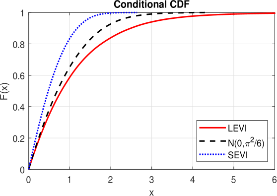
Figure S.1: CDF of the gap (absolute difference) between two above-median draws from LEVI, N$(0,\pi^{2}/6),$ and SEVI.

As a further illustration of the differences among the three distributions, Figure S.2 plots the means of $\left\{\varepsilon_{[J]}-\varepsilon_{[J-1]}\right\}$ and $\max\left\{\varepsilon_{2}-\varepsilon_{1},\ldots,\varepsilon_{J}-\varepsilon_{1}\right\}$ against $J$ when $\left\{\varepsilon_{j}\right\}_{j=1}^{J}$ is iid LEVI, $\mathrm{N}(0,\pi^{2}/6),$ or SEVI. Here, $\varepsilon_{[J]}$ and $\varepsilon_{[J-1]}$ represent the largest and second-largest values of $\left\{\varepsilon_{j}\right\}_{j=1}^{J}$, and so $\varepsilon_{[J]}-\varepsilon_{[J-1]}$ is the gap between the two largest random components. Figure S.2(a) shows that, for a given total number of alternatives, the gap is smallest under the SEVI, largest under the LEVI, and takes an intermediate value under the normal distribution. Figure S.2(b) shows that the expected maximum difference of the random components has the same ranking across the three distributions: it is the largest under the LEVI and the smallest under the SEVI. The figure indicates that, when the systematic utilities are the same across alternatives, the random components under the LEVI specification play a larger role in determining the winning choice than under the SEVI specification.

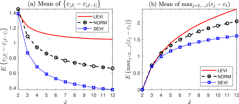
Figure S.2: The mean of the gap between the largest two random components and the mean of the maximum difference between two random components.

S.C Comparing SEVI and LEVI choice probabilities: further numerical illustrations

To further highlight the distinctions between a SEVI model and a LEVI model, we consider the case with $J=3$ so that $v=\left(v_{1},v_{2},v_{3}\right)^{\prime}.$ Define $s=\left(s_{1},s_{2},s_{3}\right)^{\prime}=\left(\exp\left(v_{1}\right),\exp\left(v_{2}\right),\exp\left(v_{3}\right)\right)^{\prime}.$ Drawing from the terminology of mathematical psychology (e.g., Yellott, (1977)), we refer to $s_{j}$ as the scale value of alternative $j.$ We create a contour plot illustrating the difference in the probabilities of choosing the first alternative (i.e., $P^{\mathrm{SEVI}}(Y=1|v)-P^{\mathrm{LEVI}}(Y=1|v)$) against $\left[s_{2},s_{3}\right],$ the scale values of the second and third alternatives for a fixed $s_{1}.$ For this fixed $s_{1},$ we also make a plot of the probability difference against $s_{2}$ while holding $s_{2}+s_{3}$ constant at a level $C,$ that is, setting $s_{3}=C-s_{2}.$ Figures S.3 and S.4 present these two plots when $v_{1}=1.5$ and so $s_{1}=\exp\left(v_{1}\right)\approx 4.5.$ Both figures demonstrate that the difference is a highly nonlinear function of $s_{2}$ and $s_{3}.$ For a given value of $s_{2}+s_{3},$ the probability difference $P^{\mathrm{SEVI}}(Y=1|v)-P^{\mathrm{LEVI}}(Y=1|v)$ depends on the relative sizes of $s_{2}$ and $s_{3}.$ Figure S.4 shows that when $s_{2}+s_{3}<\exp\left(2.193\right)\approx$ $9.0,$ so that alternative 1 has a relatively high scale value and $P^{\mathrm{LEVI}}(Y=1|v)>1/3,$ the SEVI probability is greater than the LEVI probability. Otherwise, if $s_{2}+s\geq\exp\left(2.193\right)$, alternative 1 may have a relatively low scale value, and the SEVI probability of choosing alternative 1 can be less than the LEVI counterpart. When $s_{2}+s_{3}<\exp\left(1.70\right)\approx 5.47,$ the closer $s_{2}$ and $s_{3}$ are, the stronger alternative 1 is perceived as a market leader, and the larger the difference $P^{\mathrm{SEVI}}(Y=1|v)-P^{\mathrm{LEVI}}(Y=1|v)$ becomes. In summary, in line with Figures 3–5, Figures S.3 and S.4 show that the SEVI model produces a higher choice probability for the most favored alternative but a lower choice probability for the least favored alternative than the LEVI model does.

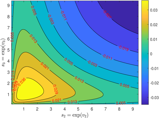
Figure S.3: Contour plot of $P^{\mathrm{SEVI}}(Y=1)-P^{\mathrm{LEVI}}(Y=1)$ against $\left[s_{2},s_{3}\right]=[\exp(v_{2}),\exp(v_{3})],$ the scale values of alternatives 2 and 3, for a fixed $s_{1}=\exp\left(1.5\right)\approx 4.5$

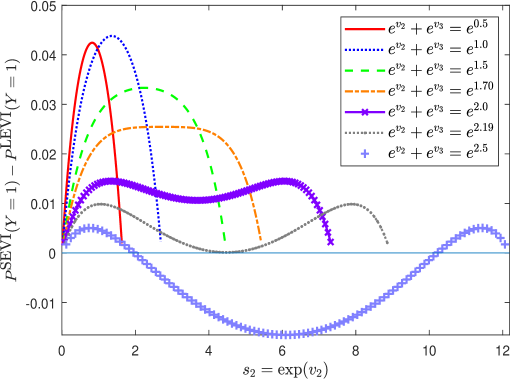
Figure S.4: Plot of $P^{\mathrm{SEVI}}(Y=1)-P^{\mathrm{LEVI}}(Y=1)$ against $s_{2}:=\exp(v_{2})$ while holding $s_{2}+s_{3}:=\exp(v_{2})+\exp(v_{3})$ constant, for a fixed $s_{1}=\exp\left(1.5\right)\approx 4.5$

Figures S.3 and S.4 are motivated by the following empirical inquiry: Imagine a market with three firms, where firm 1 is the market leader with a scale value $s_{1}=4.5$ and firms 2 and 3 have a combined scale value $s_{2}+s_{3}$ of 2.25. Under the LEVI assumption, firm 1 dominates the market with a market share of 2/3, while firms 2 and 3 together hold only 1/3. The question is, are consumers more inclined to purchase from the market leader when the other two firms have identical market power (i.e., $s_{2}=s_{3}=1.125)$, or when one of them dominates the other (e.g., $s_{2}=2$ and $s_{3}=0.25)$? The answer depends on the model used. The standard LEVI logit provides the same prediction for the dominant firm in both scenarios of competitor configurations, as in the logit case, only the sum of the competitors’ scale values matters. However, the SEVI model suggests that consumers are 4.4 percentage points more likely to choose the market leader when the remaining two firms have equal market powers; see Figure S.4. This gap between the LEVI and SEVI choice probabilities for the dominant firm narrows as the scale values of the other two firms diverge.

S.D Violation of IIA in a standard MNP

We use the same setup as discussed at the end of Section 3.4 to illustrate the violation of IIA in a standard MNP, i.e., an MNP with iid normal random utilities.

Figure S.5 is similar to Figure 6, but we plot the contour of the function below:

$$D_{\mathrm{PR}}^{\mathrm{NORM}}(s_{2},s_{3})=\frac{P^{\mathrm{NORM}}(Y=2|v_{1},v_{2},v_{3})}{P^{\mathrm{NORM}}(Y=1|v_{1},v_{2},v_{3})}-\frac{P^{\mathrm{NORM}}(Y=2|v_{1},v_{2})}{P^{\mathrm{NORM}}(Y=1|v_{1},v_{2})},$$

where $P^{\mathrm{NORM}}\left(\cdot|\cdot\right)$ denotes the choice probability under the multinomial probit with iid $N(0,\pi^{2}/6)$ errors. The figure clearly shows that $D_{\mathrm{PR}}^{\mathrm{NORM}}(s_{2},s_{3})$ is not identically zero, indicating a violation of the IIA assumption. Additionally, the figure highlights the difference between the multinomial probit model with iid $N(0,\pi^{2}/6)$ errors and the LEVI model when there are two and three alternatives. In the LEVI case, the difference in probability ratios is identically zero, providing a visual contrast with the non-zero values observed in the multinomial probit case. Therefore, caution is advised when asserting that the LEVI and MNP models yield comparable results.

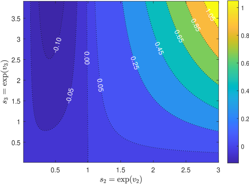
Figure S.5: Contour plot of the difference of the probability ratios $D_{\mathrm{PR}}^{\mathrm{NORM}}(s_{2},s_{3})$ against $\left[s_{2},s_{3}\right]=\left[\exp\left(v_{2}\right),\exp(v_{3})\right]$ when $s_{1}=\exp(v_{1})=1$

S.E Supplementary Figures

S.E.1 The difference between SEVI and LEVI: compensating variation and prediction probabilities

This subsection contains two figures. Figure S.6 plots the ratio of the expected compensating variation under the SEVI to that under LEVI against the alternative to be eliminated. We consider eliminating one and only one alternative at a time, and the label on the horizontal axis indicates the alternative to be removed. Figure S.7 plots the differences in the out-of-sample choice probabilities based on fitting SEVI and LEVI models when $J=4$ against the true SEVI choice probability.

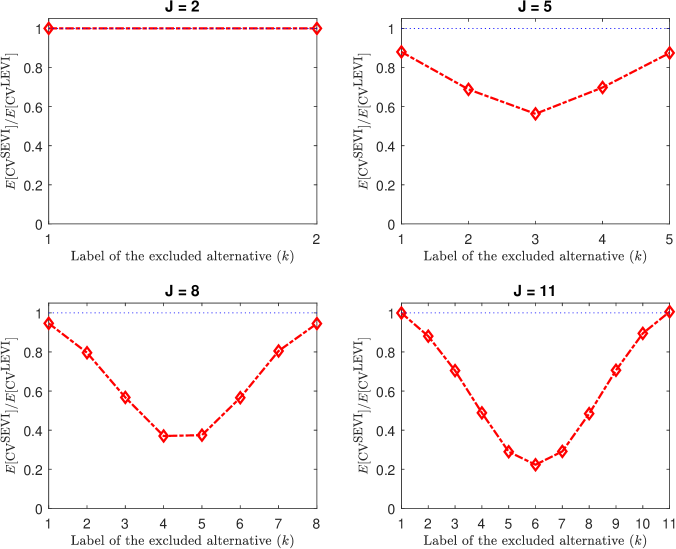
Figure S.6: Plot of the ratio of the expected compensating variations across the SEVI and LEVI models against the label of the excluded alternative with the same DGPs as those in Figure 3 ($X_{ij,\ell}$ is iid $N(0,\pi^{2}\omega_{j}^{2}/36))$

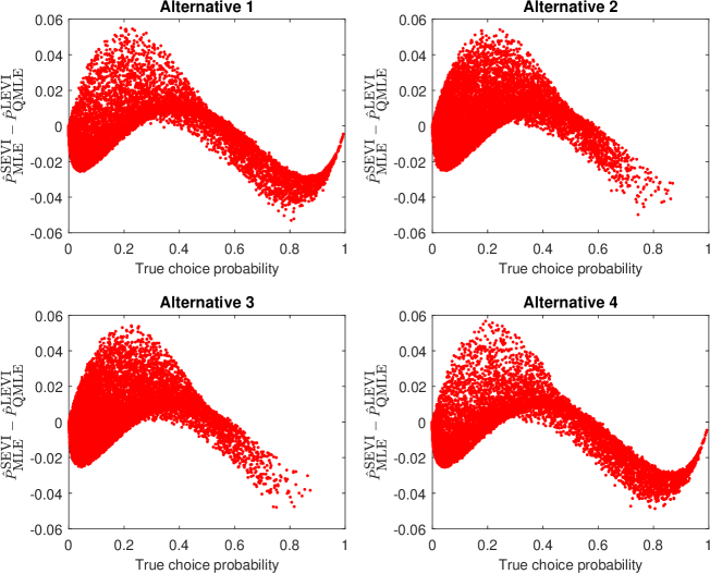
Figure S.7: Scatter plot of $\hat{P}_{i_{o},\mathrm{MLE}}^{\mathrm{SEVI}}(j)-\hat{P}_{i_{o},\mathrm{QMLE}}^{\mathrm{LEVI}}(j)$ against $P_{i_{o},0}^{\mathrm{SEVI}}\left(j\right)$ when $J=4$ and $X_{ij,\ell}\thicksim iidN(0,\pi^{2}\omega_{j}^{2}/36)$

S.E.2 Boxplot of the MLEs in a mixed LEVI-SEVI Model

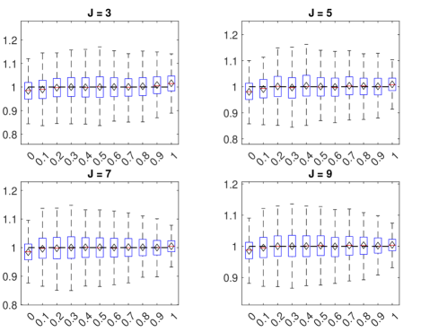
Figure S.8: Boxplot of $\hat{\beta}_{1,0}$ when the true value $\beta_{1,0}$ is $1$ against $\rho_{0}=0,0.1,...,1$, with sample size $5000$ and $J=3,5,7,9$

S.E.3 Supplementary figures: empirical applications

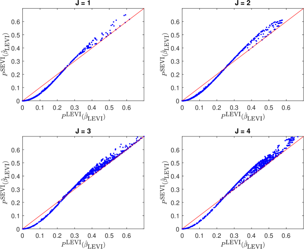
Figure S.9: Scatter plot of $P^{\mathrm{SEVI}}(\hat{\beta}_{\mathrm{LEVI}})$ against $P^{\mathrm{LEVI}}(\hat{\beta}_{\mathrm{LEVI}})$ based on the fishing mode choice data

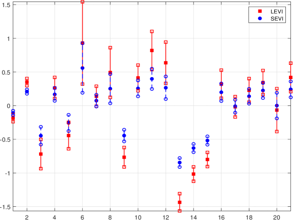
Figure S.10: Point estimates and 95% confidence intervals for the 21 parameters in the LEVI and SEVI models for the vehicle choice application

References

- Barberá and Pattanaik, (1986) Barberá, S. and Pattanaik, P. K. (1986). Falmagne and the rationalizability of stochastic choices in terms of random orderings. Econometrica, 54(3):707–715.
- Block and Marschak, (1960) Block, H. and Marschak, J. (1960). Random orderings and stochastic theories of responses. In et al., I. O., editor, Contributions To Probability And Statistics. Stanford: Stanford University Press.
- Brownstone et al., (1996) Brownstone, D., Bunch, D. S., Golob, T. F., and Ren, W. (1996). A transactions choice model for forecasting demand for alternative-fuel vehicles. Research in Transportation Economics, 4:87–129.
- Brownstone and Train, (1998) Brownstone, D. and Train, K. (1998). Forecasting new product penetration with flexible substitution patterns. Journal of Econometrics, 89(1):109–129.
- Cameron and Trivedi, (2005) Cameron, A. and Trivedi, P. (2005). Microeconometrics: Methods and Applications. Cambridge University Press.
- (6) Cameron, A. and Trivedi, P. (2022a). Analysis of Economics Data. Amazon.com.
- (7) Cameron, A. and Trivedi, P. (2022b). Microeconometrics using Stata. Stata Press, College Station, Texas.
- Chambers and Cox, (1967) Chambers, E. A. and Cox, D. R. (1967). Discrimination between alternative binary response models. Biometrika, 54(3):573–578.
- Cox, (1969) Cox, D. R. (1969). The Analysis of Binary Data. Chapman and Hall, London.
- Cramer, (2003) Cramer, J. S. (2003). Logit Models from Economics and Other Fields. Cambridge University Press, New York.
- Croissant, (2020) Croissant, Y. (2020). Estimation of random utility models in R: the mlogit package. Journal of Statistical Software, 95(11):1–41.
- Dagsvik, (2016) Dagsvik, J. K. (2016). What independent random utility representations are equivalent to the IIA assumption? Theory and Decision, 80(3):495–499.
- Daly and Zachery, (1978) Daly, A. and Zachery, S. (1978). Improved multiple choice models. In Henscher, D. and Dalvi, Q., editors, Identifying and Measuring the Determinants of Mode Choice. Teakfields, London.
- Fiebig et al., (2010) Fiebig, D. G., Keane, M. P., Louviere, J., and Wasi, N. (2010). The generalized multinomial logit model: Accounting for scale and coefficient heterogeneity. Marketing Science, 29(3):393–421.
- Fowlie, (2010) Fowlie, M. (2010). Emissions trading, electricity restructuring, and investment in pollution abatement. American Economic Review, 100(3):837–69.
- Geweke and Keane, (2001) Geweke, J. and Keane, M. P. (2001). Computationally intensive methods for integration in econometrics. In Heckman, J. J. and Leamer, E. E., editors, Handbook of Econometrics, volume 5, pages 3463–3568. Elsevier, Amsterdam.
- Greene, (2018) Greene, W. H. (2018). Econometric Analysis. Pearson, New York, 8th edition.
- Gumbel, (1958) Gumbel, E. J. (1958). Statistics of Extremes. Columbia University Press, New York.
- Hahn et al., (2020) Hahn, J., Hausman, J., and Lustig, J. (2020). Specification test on mixed logit models. Journal of Econometrics, 219(1):19–37.
- Hajivassiliou and McFadden, (1998) Hajivassiliou, V. A. and McFadden, D. (1998). The method of simulated scores for the estimation of LDV models. Econometrica, 66(4):863–896.
- Hausman and McFadden, (1984) Hausman, J. and McFadden, D. (1984). Specification tests for the multinomial logit model. Econometrica, 52(5):1219–1240.
- Hausman and Wise, (1977) Hausman, J. and Wise, D. (1977). Social experimentation, truncated distributions, and efficient estimation. Econometrica, 45(4):919–938.
- Hensher et al., (2015) Hensher, D. A., Rose, J. M., and Greene, W. H. (2015). Applied Choice Analysis: A Primer. Cambridge University Press, 2nd edition.
- Herriges and Kling, (1999) Herriges, J. A. and Kling, C. L. (1999). Nonlinear income effects in random utility models. Review of Economics and Statistics, 81(1):62–72.
- Horowitz, (1982) Horowitz, J. L. (1982). Specification tests for probabilistic choice models. Transportation Research Part A: General, 16(5-6):383–394.
- Hu, (2005) Hu, W. (2005). Logit models: smallest versus largest extreme value error distributions. Applied Economics Letters, 12(12):741–744.
- Jagelka, (2024) Jagelka, T. (2024). Are economists’ preferences psychologists’ personality traits? a structural approach. Journal of Political Economy, 132(3):910–970.
- Jain et al., (1994) Jain, D. C., Vilcassim, N. J., and Chintagunta, P. K. (1994). A random-coefficients logit brand-choice model applied to panel data. Journal of Business & Economic Statistics, 12(3):317–328.
- Jiang et al., (2024) Jiang, Z., Peng, C., and Yan, H. (2024). Personality differences and investment decision-making. Journal of Financial Economics, 153:103776.
- Keane and Wolpin, (1994) Keane, M. P. and Wolpin, K. I. (1994). The solution and estimation of discrete choice dynamic programming models by simulation and interpolation: Monte Carlo evidence. Review of Economics and Statistics, 76(5):648–672.
- Knuth, (2011) Knuth, D. (2011). The Art of Computer Programming, Volume 4A: Combinatorial Algorithms, Part 1. Pearson Education, Hoboken, NJ.
- Lindberg and Smith, (2017) Lindberg, P. O. and Smith, T. (2017). A note on a recent paper by Dagsvik on IIA and random utilities. Theory and Decision, 82(2):305–307.
- Luce, (1959) Luce, R. D. (1959). Individual Choice Behavior: A Theoretical Analysis. Wiley.
- Mai et al., (2017) Mai, T., Bastin, F., and Frejinger, E. (2017). On the similarities between random regret minimization and mother logit: The case of recursive route choice models. Journal of Choice Modelling, 23(C):21–33.
- Manski, (1977) Manski, C. F. (1977). The structure of random utility models. Theory and Decision, 8(3):229–254.
- McFadden, (1973) McFadden, D. (1973). Conditional logit analysis of qualitative choice behaviour. In Zarembka, P., editor, Frontiers in Econometrics, pages 105–142. Academic Press, New York, NY, USA.
- McFadden, (1981) McFadden, D. (1981). Econometric models of probabilistic choice. In Manski, C. F. and McFadden, D., editors, Structural Analysis of Discrete Data with Econometric Applications, pages 198–272. MIT Press.
- McFadden, (2001) McFadden, D. (2001). Economic choices. American Economic Review, 91(3):351–378.
- McFadden and Train, (2000) McFadden, D. and Train, K. (2000). Mixed MNL models for discrete response. Journal of Applied Econometrics, 15(5):447–470.
- McFadden et al., (1978) McFadden, D., Train, K., and Tye, W. (1978). An application of diagnostic tests for the irrelevant alternatives properties of the multinomial logit model. Transportation Research Record, 637:39–46.
- Paap and Franses, (2000) Paap, R. and Franses, P. H. (2000). A dynamic multinomial probit model for brand choice with different long-run and short-run effects of marketing-mix variables. Journal of Applied Econometrics, 15(6):717–744.
- Ross, (2013) Ross, S. (2013). A First Course in Probability. Pearson.
- Ruud, (1986) Ruud, P. A. (1986). Consistent estimation of limited dependent variable models despite misspecification of distribution. Journal of Econometrics, 32(1):157–187.
- Strzalecki, (2023) Strzalecki, T. (2023). Stochastic Choice Theory. preprint, Department of Economics, Harvard University. https://scholar.harvard.edu/sites/scholar.harvard.edu/files/tomasz/files/scnotes94k.pdf.
- Sørensen and Fosgerau, (2022) Sørensen, J. R.-V. and Fosgerau, M. (2022). How McFadden met Rockafellar and learned to do more with less. Journal of Mathematical Economics, 100:102629.
- Thurstone, (1927) Thurstone, L. L. (1927). A law of comparative judgment. Psychological Review, 34(4):273–286.
- Train, (2009) Train, K. (2009). Discrete Choice Methods with Simulation. Cambridge University Press, 2nd edition.
- Vuong, (1989) Vuong, Q. H. (1989). Likelihood ratio tests for model selection and non-nested hypotheses. Econometrica, 57(2):307–333.
- Williams, (1977) Williams, H. (1977). On the formulation of travel demand models and economic measures of user benefit. Environment & Planning A: Economy and Space, 9(3):285–344.
- Wooldridge, (2002) Wooldridge, J. M. (2002). Econometric Analysis of Cross Section and Panel Data. MIT Press, Cambridge and London.
- Yellott, (1977) Yellott, J. I. (1977). The relationship between Luce’s choice axiom, Thurstone’s theory of comparative judgment, and the double exponential distribution. Journal of Mathematical Psychology, 15(2):109–144.