Barren plateaus induced by the dimension of qudits

Abstract

Variational Quantum Algorithms (VQAs) have emerged as pivotal strategies for attaining quantum advantages in diverse scientific and technological domains, notably within Quantum Neural Networks. However, despite their potential, VQAs encounter significant obstacles, chief among them being the gradient vanishing problem, commonly referred to as barren plateaus. In this study, we unveil a direct correlation between the dimension of qudits and the occurrence of barren plateaus, a connection previously overlooked. Through meticulous analysis, we demonstrate that existing literature implicitly suggests the intrinsic influence of qudit dimensionality on barren plateaus. To fortify these findings, we present numerical results that exemplify the impact of qudit dimensionality on barren plateaus. Additionally, despite the proposition of various error mitigation techniques, our results call for further scrutiny about their efficacy in the context of VQAs with qudits.

I Introduction

While quantum computing has roots in the past Nielsen2010 , its substantial expansion has primarily unfolded in recent years Nature2022 . Both companies and governmental entities have made substantial investments in hardware, software, and human capital to propel the advancement of these quantum devices Riedel2019 ; Monroe2019 . The pursuit of quantum computers is driven by their envisioned superiority over classical counterparts. A prominent illustration of this potential is Shor’s algorithm Shor , which was meticulously crafted for prime number factorization. This algorithm bears the capability to efficiently break cryptographic keys, thus holding profound implications across various societal realms, particularly in an interconnected world where privacy stands as a cornerstone.

While Shor’s algorithm has historically been a driving force behind quantum computing development, the contemporary landscape, characterized by Noisy Intermediate-Scale Quantum devices (NISQ) Preskill , has ushered in Variational Quantum Algorithms (VQAs) as the forefront strategy for achieving quantum advantages Cerezo_VQA . These algorithms have garnered attention due to their potential to surpass classical computing methodologies. VQAs have already found applications in diverse fields, including chemical reaction simulations BAUER2020 , optimization Cerezo_VQA , and machine learning quantum_model_multilayer_perception ; kernel_methods ; quantum_Convolutional ; hybrid_1 ; hybrid_2 ; hybrid_3 ; hybrid_4 . Their versatility and efficacy in tackling intricate problems underscore their significance across a spectrum of domains.

Despite promising advancements, Variational Quantum Algorithms encounter several challenges, among which barren plateaus (BPs) stand out as a significant issue. In VQAs, a classical optimizer is employed to adjust the parameters of a quantum circuit, aiming to minimize a cost function. Typically, gradient-based methods are used to optimize these parameters, leveraging the gradient of the cost function. However, the presence of barren plateaus causes the gradient to diminish as the number of qubits increases, hindering the training process of VQAs and, as a result, constraining their practical application.

Several factors have been associated with the problem of barren plateaus, including the choice of the cost function barrenPlateaus_1 , the expressibility of the quantum circuit barrenPlateaus_2 , entanglement barrenPlateaus_4 ; barrenPlateaus_5 , and noise barrenPlateaus_3 . Despite research efforts to address this problem, our understanding of the phenomenon is still limited. For example, some approaches propose the use of optimization methods where the gradient of the cost function is not employed to adjust the parameters of the quantum circuit Friedrich_Evolution_strategies ; lles ; ANAND . However, studies have shown that even these methods are not immune to barren plateaus barrenPlateaus_6 . As a result, other studies have been conducted to propose ways to mitigate barren plateaus barrenPlateaus_7 ; barrenPlateaus_8 ; barrenPlateaus_9 ; barrenPlateaus_10 ; barrenPlateaus_11 ; Friedrich_ensemble_learning , highlighting the complexity and ongoing importance of this research area.

Quantum computers function by manipulating two-level systems known as qubits Nielsen2010 , which are analogous to the bits used in classical computing. Similar to bits, qubits possess two possible states, typically denoted as 0 or 1. However, unlike bits, each qubit can exist in a superposition of these states, allowing it to simultaneously represent both the 0 and 1 states. This property, known as superposition, is one of the fundamental characteristics that enable the quantum advantage to be achieved.

Although the leading quantum computers currently in development are designed using qubits, an alternative quantum information processing strategy is to utilize qudits. Qudits are a generalization of qubits, representing systems with a greater number of possible states, usually denoted as $d$ levels. Recent studies have explored the use of qudits in quantum computing CHI2022 , including the development of quantum machine learning algorithms based on variational quantum algorithms (VQAs) ROCA2023 ; WACH2023 ; VALTINOS2023 . However, this is an area of study in its early stages, and therefore our understanding of the applicability of VQA models using qudits is still limited, with several questions yet to be explored.

In this work, we present a new perspective on the BPs problem, examining its relationship with the dimension of qudits and introducing the concept of ‘barren plateaus induced by the dimension of qudits’. Our investigation indicates that an increase in the dimensionality of qudits correlates with a heightened impact of BPs on VQAs. Consequently, while the adoption of qudits in quantum computing presents potential benefits, the dimensional characteristics of qudits substantially affect the trainability and viability of VQAs in practical applications.

This work is organized as follows. We begin by presenting a brief summary of Variational Quantum Algorithms in Section II. Next, in Section III, we delve into the problem of barren plateaus. Then, in Section IV, we introduce qudits. In Section V, we present our main theoretical results, followed by numerical results in Section VI. We conclude our findings in Section VII. At last, Appendix A is used to give a detailed proof of Theorem 1.

II Variational quantum algorithms

Variational Quantum Algorithms (VQAs) are emerging as a promising approach in quantum computing, offering a flexible and adaptable framework to address a wide array of complex challenges, particularly within the realm of Noisy Intermediate-Scale Quantum devices (NISQ). These devices, characterized by their smaller-scale systems, confront significant hurdles related to noise and limited qubit coherence. In a typical VQA, a parameterized quantum circuit is employed to represent a family of quantum states, with its parameters iteratively adjusted by a classical optimization algorithm. The objective is to minimize a cost function associated with a specific problem, enabling the quantum circuit to adapt and approximate the optimal solution.

In general, the cost function is defined as follows:

$$C(\boldsymbol{\theta})=Tr[OU(\boldsymbol{\theta})\rho U(\boldsymbol{\theta})^{\dagger}],$$ (1)

where $\rho$ represents the system initial state, $O$ is a Hermitian operator describing an observable, and $U(\boldsymbol{\theta})$ denotes any parametrization dependent on the parameters $\boldsymbol{\theta}$ to be optimized.

Usually, we can define $O$ locally or globally, and, as we will see in Section III, its choice has serious implications for the trainability of the model. On the other hand, the parameterization $U(\boldsymbol{\theta})$ can take on a multitude of forms, which defines how the quantum gates are distributed in a quantum circuit. For example, in quantum neural networks, what generally distinguishes all the proposed models quantum_model_multilayer_perception ; kernel_methods ; quantum_Convolutional ; hybrid_1 ; hybrid_2 ; hybrid_3 ; hybrid_4 is precisely the way this parameterization is obtained. Some studies have already proposed to investigate how this choice can influence the model’s performance Friedrich_chip . In Refs. RAGONE2022 ; LAROCCA2022 , for example, it was analyzed how to construct this parameterization based on the symmetries of the training data in the context of quantum neural networks. However, in general, this parameterization is defined as:

$$U(\boldsymbol{\theta})=\prod_{l=1}^{L}U_{l}=\prod_{l=1}^{L}U_{l}(\boldsymbol{\theta}_{l})W_{l},$$ (2)

where $U_{l}(\boldsymbol{\theta}_{l})$ is a parameterization obtained from applying a sequence of quantum gates depending on the parameters $\boldsymbol{\theta}_{l}$. The operations $W_{l}$ are another parameterizations, also obtained from applying a sequence of quantum gates, but not depending on parameters $\boldsymbol{\theta}_{l}$, and $L$ is the depth of the parameterization $U$.

The objective of classical optimization is to obtain the parameters $\boldsymbol{\theta}^{\ast}$ such that:

$$\boldsymbol{\theta}^{\ast}=\arg_{\boldsymbol{\theta}}\min C(\boldsymbol{\theta}),$$ (3)

meaning that $C(\boldsymbol{\theta})$ attains its smallest possible value. Although several optimization methods have been proposed Friedrich_Evolution_strategies ; lles ; ANAND , generally, this optimization is performed using gradient-based methods. For instance, the gradient descent method involves updating the parameters of the parameterization using the gradient of the cost function. This method is described by the following optimization rule:

$$\boldsymbol{\theta}^{t+1}=\boldsymbol{\theta}^{t}-\eta\big{(}\nabla_{\boldsymbol{\theta}}C(\boldsymbol{\theta})\big{)}_{\theta^{t}},$$ (4)

where $\eta$ is the learning rate. As mentioned, this is an iterative method where the parameters of $U$ are optimized to minimize the cost function; thus, $t$ refers to the current epoch.

III Barren Plateaus

The problem of gradient vanishing in parameterized quantum circuits, also known a barren plateaus, was initially introduced in Ref. barrenPlateaus_0 in the context of quantum neural networks. In this pioneering work, the authors first demonstrated that the gradient of the cost function, used to optimize the parameters of the parameterization, exponentially decreases with the number of qubits used in the quantum circuit. Although it was observed that this problem is also related to the depth $L$ of the parameterization, it was only in Ref. barrenPlateaus_1 that theoretical results showing this relationship were obtained. The barren plateaus are defined as follows.

Definition 1

Let the cost function be defined in Eq. (1), with $O$ being any observable, $\rho$ the initial state of $n$ qubits, and $U$ the parameterization given in Eq. (2). We say that this function exhibits barren plateaus if

$$Var[\langle\partial_{k}C\rangle]\leqslant G(n)\propto\mathcal{O}\bigg{(}\frac{1}{b^{n}}\bigg{)},\ b>1.$$ (5)

This definition is obtained from Chebyshev’s inequality:

$$Pr(|\partial_{k}C-\langle\partial_{k}C\rangle|\geqslant\delta)\leqslant\frac{Var[\langle\partial_{k}C\rangle]}{\delta^{2}},$$ (6)

which states that the probability that the partial derivative of the cost function with respect to any parameter $\theta_{k}$ deviates from its mean $\langle\partial_{k}C\rangle$ by a value greater than or equal to $\delta$ will be bounded by $Var[\langle\partial_{k}C\rangle]$. As shown in Refs. barrenPlateaus_0 ; barrenPlateaus_1 , it follows that:

$$\langle\partial_{k}C\rangle=0\ \forall k.$$ (7)

Therefore, the inequality in Eq. (6) informs us about the probability of $\partial_{k}C$ deviating from the value $0$. As a consequence, the smaller the value of the variance, the more the value of the derivative $\partial_{k}C$ will concentrate around zero. Therefore, its trainability and consequent applicability can be severely hindered.

Several results in the literature have already related barren plateaus to different properties barrenPlateaus_0 ; barrenPlateaus_1 ; barrenPlateaus_2 ; barrenPlateaus_3 ; barrenPlateaus_4 ; barrenPlateaus_5 , such as expressiveness, which is related to the capacity of the parameterization $U$ to access the Hilbert space. The greater its capacity to access this space, the more expressive it will be. For example, in Ref. barrenPlateaus_2 the authors analyze the relationship between expressiveness and barren plateaus. They showed that the higher the expressiveness of the parameterization, the greater will be its affects on barren plateaus. Recently, several studies have aimed to analyze how VQAs are affected by expressiveness FRIEDRICH_Expre_2023 ; SIM2019 ; HUBREGTSEN2021 .

In Ref. barrenPlateaus_1 , the authors analyzed how barren plateaus can be influenced by the choice of the cost function. The cost function from Eq. (1) depends on $O$, which generally can be any observable. The authors investigated how the choice of this observable affects barren plateaus. They considered two different types of observables: global observables and local observables. A global observable is defined so that the value of the cost function depends on the simultaneous measurement of all qubits. On the other hand, a local observable is defined when the value of the cost function depends only on the measurement of one qubit or some pairs of qubits. As shown in Ref. barrenPlateaus_1 , the cost function will not exhibit the problem of barren plateaus in the second case, of local observables, if the relationship between the depth of the parameterization and the number of qubits is $\mathcal{O}(1)$ or $\mathcal{O}(\log(n))$. However, for the first case, of global observables, the cost function will always exhibit the problem of barren plateaus.

IV Qudits

Qudits represent a generalization of qubits, where a qubit is a particular case of a qudit with dimension $d=2$. A $d$-dimensional qudit state can be described in terms of the standard basis $\{|0\rangle,|1\rangle,\cdots,|d-1\rangle\}$:

$$|\psi\rangle=\sum_{l=0}^{d-1}\alpha_{l}|l\rangle,$$ (8)

with $\sum_{l=0}^{d-1}|\alpha_{l}|^{2}=1$. Although neutral multilevel Rydberg atoms or molecular magnets may be considered the best candidates for implementing qudits Weggemans2022 , most advancements in quantum information have been achieved using photons Wang2023 . In these cases, the qudit’s state is represented by a single photon superposed over $d$ modes, which can be spatial, temporal, frequency, or orbital angular momentum modes.

In quantum computing based on qubits, the state $|\psi\rangle$ describing a system of $n$ qubits is manipulated through quantum operations, such as the Hadamard gate, CNOT gate, and rotation gates, among others Wang2020 . With appropriate adjustments, it is also possible to define quantum gates specifically designed to work with systems involving qudits. For instance, for the purposes of this work, two gates that can be adapted to operate with qudits are the rotation gate

$$R_{jk}^{\alpha}=e^{-i\theta S_{\alpha}^{jk}/2},$$ (9)

where the generalized Gell-Mann matrices are GGM

$$S_{x}^{jk}=|j\rangle\langle k|+|k\rangle\langle j|\text{ with }1\leqslant j<k\leqslant d^{\prime},$$ (10)

$$S_{y}^{jk}=-i|j\rangle\langle k|+i|k\rangle\langle j|\text{ with }1\leqslant j<k\leqslant d^{\prime},$$ (11)

$$S_{z}^{j}=\sqrt{\frac{2}{j(j+1)}}\sum_{k=1}^{j+1}(-j)^{\delta(k,j+1)}|k\rangle\langle k|,$$ (12)

with $1\leqslant j\leqslant d^{\prime}-1$ for $S_{z}^{j}$, and the CNOT gate

$$CNOT|x\rangle|y\rangle=|x\rangle|x+y(\bmod d)\rangle,$$ (13)

with $x,y=0,\cdots,d-1.$

Although promising, quantum computers are predominantly in the development phase, focusing on qubit operations. Furthermore, the potential use of qudits in solving VQA problems is an emerging area, and our theoretical foundations are still considerably limited. In the next section, we aim to expand these foundations by examining how barren plateaus are influenced by the dimension of qudits.

V Barren plateaus in qudit systems

In this section, we will discuss how BPs are induced by the dimension of qudits. To do so, we begin by presenting the following definition:

Definition 2

(Barren plateaus induced by the dimension of the qudits) Let the cost function be defined in Eq. (1) with $U$ given by Eq. (2) and $O$ any observable. We say that this function suffers from dimension-induced BPs if

$$Var[\langle\partial_{k}C\rangle]\leqslant F(n,d^{\prime})\propto\mathcal{O}\bigg{(}\frac{1}{d^{\prime n}}\bigg{)},$$ (14)

with $d^{\prime}\geqslant 2$ being the dimension of the qudits and $n$ the number of qudits.

Thus, alike to Definition 1, the Definition 2 is obtained from Chebyshev’s inequality and tells us that if the variance decreases as the dimension $d^{\prime}$ of the qudits increases, then the VQA will suffer from dimension-induced barren plateaus.

To prove the qudit-induced barren plateaus, we will consider the formalism of $t-$designs. The $t-$designs are defined as follows: Consider a finite set $\{W_{y}\}_{y\in Y}$ (of size $|Y|$) of unitaries with a Hilbert space of dimension $d$. If $P_{(t,t)}(W)$ is an arbitrary polynomial of degree at most $t$ in the elements of the matrix of $W$ and at most $t$ in $W^{\dagger}$, and

$$\frac{1}{|Y|}\sum_{y\in Y}P_{(t,t)}(W_{y})=\int_{U(d)}d\mu(W)P_{(t,t)}(W),$$ (15)

we say that this finite set is a $t-$design. This result implies that the average of $P_{(t,t)}(W)$ over the $t-$design is indistinguishable from integration over $U(d)$ with respect to the uniform-Haar distribution 2_design .

From this definition of $t-$design, we are able to derive several lemmas that are useful when obtaining theoretical results showing that indeed the variance of the partial derivative of the cost function in Eq. (1) decreases as the number of qubits increases. However, we also observe that we can use this definition of $t-$design to show that the dimension of qudits also induces barren plateaus. To do so, we simply observe that this definition holds for any set of unitaries of degree $d$.

The variable $d$ is commonly defined as $d=2^{n}$, where $n$ represents the number of qubits used in the VQA, and the base $2$ corresponds to the binary dimensionality inherent to qubits. When extending this framework to accommodate qudits, the primary modification involves substituting the base $2$ with the dimension $d^{\prime}$ of the qudits. Consequently, $d$ is redefined as $d=d^{\prime n}$. This adaptation allows the application of existing lemmas that explore the relationship between variance and the number of qubits to also assess the impact of qudit dimensionality.

To analyze how the variance behaves as the dimension $d^{\prime}$ of the qudits increases, we must first obtain an expression for the derivative of $C$. To do so, we start by rewriting the parameterization $U$ given by Eq. (2) as:

$$U=U_{L}U_{R},$$ (16)

with

$$U_{L}=\prod_{l=1}^{p-1}U_{l}W_{l}$$ (17)

and

$$U_{R}=\prod_{l=p}^{L}U_{l}W_{l},$$ (18)

where $U_{l}$ will be given by

$$U_{l}=\bigotimes_{m=1}^{n}R_{jk}^{\alpha}(\theta_{ml}).$$ (19)

Thus, from Eq. (1), we have

$$\partial_{k}C=\frac{\partial C}{\partial\theta_{qp}}=\frac{i}{2}Tr\bigg{[}U_{L}^{\dagger}OU_{L}\big{[}U_{R}\rho U_{R}^{\dagger},[I_{q}\otimes S_{\alpha}^{jk}]\big{]}\bigg{]},$$ (20)

where $S_{\alpha}^{jk}$ is given by Eqs. (10), (11), and (12). For more details on obtaining this derivative, see Appendix A.

With this derivative, we can see that if $U_{L}$ or $U_{R}$ form a $1$-design, then

$$\langle\partial_{k}C\rangle=0\text{ }\forall k.$$ (21)

Therefore, the smaller $Var[\partial_{k}C]$, the closer $\partial_{k}C$ will be to the value $0$, making it difficult to train the model. The same holds if $U_{L}$ and $U_{R}$ simultaneously form a $1$-design. For more details on how to obtain this result, see Appendix A. Next, we will present Theorem 1, which relates the variance of $\partial_{k}C$ to the dimension $d^{\prime}$ of the qudits.

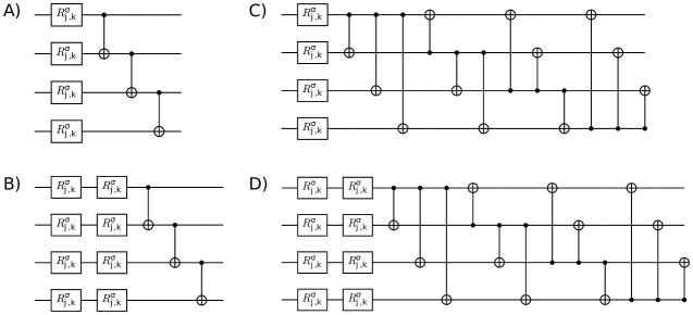
Figure 1: Illustration of the parameterizations used in this work. In this figure, each parameterization shows the form of the unitary $U_{l}$ used in Eq. (2). For parameterizations A and B, the CNOT gate is applied only between neighboring pairs of qudits, while in the parameterizations C and D it is applied between all pairs of qudits. In all these parameterizations, rotation gates $R^{\sigma}_{(j,k)}$ are applied to all qudits. The pair of variables $(j,k)$ are the indices of the Gell-Mann matrices, that we randomly choose. Moreover, $\sigma$ indicates which axis the rotation gate will be applied to, with $\sigma=X,Y,Z$. During the simulations, the $\sigma$ values are also chosen at random.

Theorem 1

Let the cost function be defined in Eq. (1), with $O$ being any observable, $\rho=|\psi\rangle\langle\psi|$ an initial state, and $U$ the parameterization defined in Eq. (2), with $U_{l}$ given by Eq. (19). Then the variance of the partial derivative of the cost function in Eq. (1) with respect to any parameter $\theta_{k}$ will be:

$$Var[\partial_{k}C]=\frac{d^{\prime(n-1)}}{d+1}\bigg{(}\frac{Tr[O^{2}]}{d^{2}-1}-\frac{Tr[O]^{2}}{d(d^{2}-1)}\bigg{)},$$ (22)

where $d=d^{\prime n}$ with $d^{\prime}$ being the dimension of the qudits and $n$ the number of qudits used in the model.

The proof of this theorem is presented in Appendix A.

Corollary 1

Let the cost function be defined in Eq. (1) with $O=|0\rangle\langle 0|$. From Theorem 1, we have:

$$Var[\partial_{k}C]=\frac{1}{d^{\prime}(d^{\prime n}+1)^{2}}.$$ (23)

Therefore, from this result, we see that the variance will decrease as the dimension $d^{\prime}$ of the qudits used in the VQA increases.

VI Results

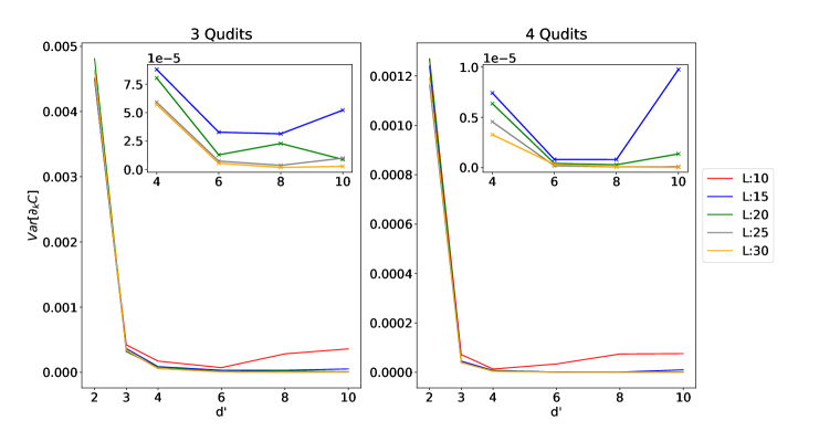
Figure 2: Behavior of the variance of the cost function, Eq. (1), with $O=|0\rangle\langle 0|$ and parameterization $U$, Eq. (2), with $U_{l}$ given by Fig. 1A. In this case, we can see that for sufficiently large $L$, the behavior of the variance is in accordance with Theorem 1. However, for low values of $L$, specifically for $L=10$ and $L=15$, we can see that the behavior of the variance differs from what is expected according to Theorem 1. As we will discuss later, this happens because the parameterization set $U$ generated does not form an exact $t$-design but rather an approximation. So, it is expected that the behavior of the variance differs from the theoretical result.

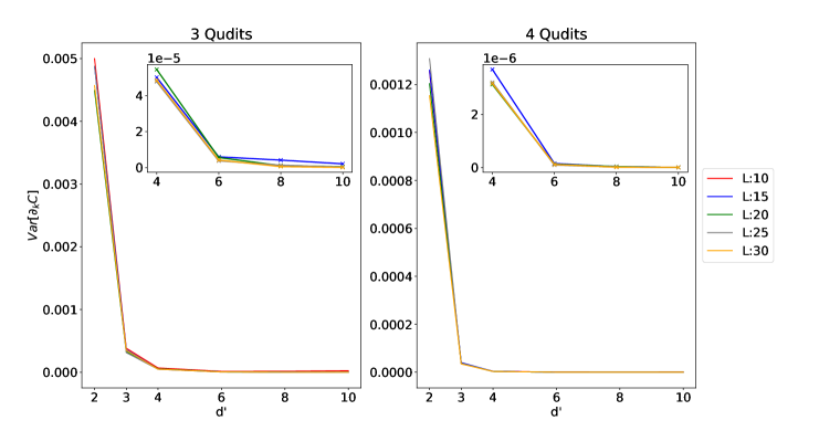
Figure 3: Behavior of the variance of the cost function, Eq. (1), with $O=|0\rangle\langle 0|$ and parameterization $U$, Eq. (2), with $U_{l}$ shown in Fig. 1 B. In contrast to the previous case (Fig. 2), here the behavior of the variance of the cost function is in accordance with Theorem 1 in all cases.

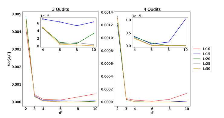
Figure 4: Behavior of the variance of the cost function for $U_{l}$ given by Fig. 1C. Similar to the case seen in Fig. 2, for relatively low values of $L$, the behavior of the variance differs from what is expected according to Theorem 1.

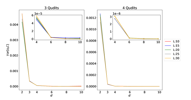
Figure 5: Behavior of the variance of the cost function for the parameterization obtained using $U_{l}$ shown in Fig. 1D. Again, we use $O=|0\rangle\langle 0|$. As we can observe immediately, similar to the case seen in Fig. 3, the behavior of $Var[\partial_{k}C]$ is in accordance with Theorem 1 in all cases analyzed.

In this section, we present the numerical results confirming our theoretical findings, demonstrating numerically that indeed the dimension of the qudits induces the problem of barren plateaus. To perform these simulations, we used the PyTorch library Paszke to implement a series of operations involving VQAs with qudits. For more details about these operations, please refer to the code provided at the link appearing in the Data Availability statement.

For these results, we used the general form of parameterization given by Eq. (2), where $U_{l}$ is determined by the parameterizations illustrated in Fig. 1. All these parameterizations depend on the CNOT gate and on the rotation gate $R^{\sigma}_{j,k}$ with $\sigma=X,Y,Z$.

The variance of $\partial_{k}C$ with respect to each $U_{l}$ illustrated in Figure 1 was obtained following a specific process. Initially, we selected the desired form to generate $U_{l}$. Then, we generated 2000 random parameterizations $U$ to calculate the variance of $\partial_{k}C$. Each of these parameterizations $U$ was obtained as follows: first, we defined a depth $L$ and the number of qudits to be used in the parameterization. Subsequently, we determined the dimension $d^{\prime}$ of the qudits. Next, we randomly selected each rotation gate used in the parameterization, i.e., we chose $\sigma$ randomly in the set $\{X,Y,Z\}$. If $\sigma$ was chosen as $X$ or $Y$, we randomly generated the pair of variables $(j,k)$ such that $1\leqslant j<k\leqslant d^{\prime}$. In the case where $\sigma=Z$, we randomly generated $j$ such that $1\leqslant j\leqslant d^{\prime}-1$. Finally, we generated the parameters $\boldsymbol{\theta}$ from a uniform distribution in the interval $[0,2\pi]$. With these parameters, we calculated the derivative $\partial_{k}C$ for $k=(1,1)$, i.e., the derivative with respect to the rotation gate acting on the first qudit of the first layer.

As an observable, we chose $O=|0\rangle\langle 0|$. Thus, from Corollary 1, we know that the variance in this case tends to decrease as the dimension $d^{\prime}$ of the qudits increases. In the following results, we explore different values of $L$, aiming to analyze how the variance is affected by the depth of the parameterization. Additionally, we focus on analyzing the behavior of the variance for parameterizations obtained using $3$ and $4$ qudits. This limited selection is justified for two main reasons. Firstly, our central goal is to demonstrate that barren plateaus are induced by the dimension of the qudits, so our results focus on analyzing the relationship between the variance of $\partial_{k}C$ and the dimension of the qudits. Secondly, hardware limitations also play a significant role. Generally, when performing VQA simulations on classical computers, the maximum number of qubits we can simulate is already limited due to the exponential growth of computational resources required as the number of qubits increases. In the case of qudits, this challenge is even greater, especially for relatively large values of $d^{\prime}$.

Figure 2 illustrates the behavior of the variance for the parametrization $U_{l}$ as depicted in Figure 1A. It is evident that the variance generally decreases with an increase in the qudit dimension $d^{\prime}$, particularly for $L=25$ and $L=30$. However, in scenarios where $L=10,15,\text{ and }20$, the variance predominantly decreases, yet there are instances where it unexpectedly increases. Two primary hypotheses are proposed to explain this phenomenon:

1. The number of generated parameterizations $U$ to calculate the variance is limited. In fact, the possible number of parameterizations is practically unlimited, mainly because each parameter $\theta_{k}$ is a continuous value. Therefore, even though we used 2000 parameterizations, this is still a very low number. As a result, the obtained variance is an under-sampled estimate.

2. The theoretical results are based on the assumption that the set of generated parameterizations $U$ forms a $t-$design. However, this set does not form an exact $t-$design but rather an approximation. Therefore, it is expected that for these cases, the variance differs from the theoretical results.

Regarding the number of qudits, although we only used two values, it is possible to see that the variance using $4$ qudits is lower than the one obtained using $3$ qudits. This is in accordance with Theorem 1, where we observe that indeed the number of qudits will influence the variance, and the larger this number of qudits is, the lower will be the variance.

Figure 3 shows the behavior of the variance for the parametrization illustrated in Figure 1B. In contrast to the previous case, where an increase in variance was observed in some instances, in this case all variances decreased as the dimension $d^{\prime}$ of the qudits increased. Additionally, we noticed that the variance with $4$ qudits is lower than the variance with $3$ qudits. Therefore, in this case, the behavior of the variance is in complete agreement with the expected results according to Theorem 1.

Next, in Figure 4, we analyze the behavior of the variance in the case where the parametrization $U_{l}$ is illustrated in Figure 1C. Immediately, we observe that, similar to the case shown in Figure 2, there were instances where the variance increased when it was expected to decrease. Again, the two possible explanations for this behavior are: the number of $U$ parametrizations used to calculate the variance is insufficient, which can lead to under-sampling; or the fact that the set of unitaries obtained does not form an exact $t-$design, but rather an approximation, which can result in a variance diverging from the expected theoretical result. Additionally, we observe that for sufficiently large values of $L$, the behavior of the variance is in accordance with Theorem 1, and the variance with 4 qudits was lower than the variance obtained with 3 qudits, as expected.

Finally, in Figure 5, we observe the behavior of the variance for the case where $U_{l}$ was given by Figure 1D. Initially, we note that in all cases the variance decreased as the dimension $d^{\prime}$ of the qudits increased, and the variance obtained when using 4 qudits is lower than that obtained when using 3 qudits. Thus, we can conclude that the variance behaved as expected by Theorem 1.

As we have seen, there were cases, Figures 2 and 4, where the behavior of the variance was different from what was expected according to Theorem 1. Initially, we presented two possible explanations for this behavior. However, upon analyzing all the results obtained, we can conclude that the best explanation for this behavior is that the set of unitaries generated does not form, in these cases, an exact $t-$design but rather an approximation. Therefore, it is expected that the behavior of the variance differs from the theoretical result.

To justify this conclusion, we first ruled out the first possible explanation, which is based on statistical under-sampling due to the limited number of $U$ parametrizations used to calculate the variance. However, if this was the case, then the same behavior should be observed in Figures 3 and 5. Additionally, we should see a much more complex behavior for the cases shown in Figures 3 and 5 if this were the correct explanation, because in these cases the total number of possible parametrizations is higher than the total number for the parametrizations obtained using Figs. 1A and 1C, thus the numerical error should be more evident for these cases.

With the possibility of under-sampling ruled out, another hypothesis is that the set of unitaries does not form an exact $t-$design. So it is expected that the behavior of the variance differs from the theoretical result.

VII Conclusions

Recently, some studies have proposed the use of variational quantum algorithms (VQAs) with qudits to solve machine learning problems. Although this approach is promising, it is still in its early stages of development. As a result, our understanding of issues such as the trainability of these models is still limited. In this work, our goal was to analyze how VQAs using qudits are affected by barren plateaus (BPs). By using the formalism of $t-$designs, we observed BPs arising due to the dimension of the qudits. This comes from the fact that, from the formalism of $t-$designs, we observe a dependence on the dimension $d$ of the Hilbert space. This dimension is $d=2^{n}$ for qubits. However, for qudits, we can generalize this dimension to $d=d^{\prime n}$, where $d^{\prime}$ represents the dimension of the qudits.

Based on this analysis, we derived Theorem 1, which establishes a relationship between the variance of the partial derivative of the cost function and the dimension $d^{\prime}$ of the qudits. To confirm this result, we conducted a series of numerical experiments in which we analyzed how the variance of the partial derivative of the cost function behaves for different values of $d^{\prime}$, using various parameterizations. The results obtained confirm that indeed, barren plateaus are induced by the dimension of qudits.

Furthermore, the results obtained allow us to open a discussion on how the mitigation methods proposed so far can be applied in this specific case. Generally, these methods aim to increase the variance of the cost function. For example, consider a problem that can be solved by a VQA using $L$ layers and $n$ qubits, and suppose that, for this specific case, the variance is equal to a value $x$. Typically, mitigation methods simply increase this value to $x+\delta$, where $\delta\ll 1$. However, when using a VQA with qudits, we observe that the value of the variance is significantly lower than that obtained with a VQA with qubits. This leads us to question whether this value $\delta$ is really sufficient to mitigate the problem of Barren plateaus, or if it simply moves us from one region of barren plateaus caused by a certain dimension $d^{\prime}$ to another region of Barren plateaus caused by another dimension $d^{\prime\prime}$, where $d^{\prime\prime}<d^{\prime}$.

Therefore, in this work, besides identifying a new cause for the emergence of barren plateaus, we also demonstrate that, although the use of VQAs with qudits may represent a promising path for solving various problems, their trainability and consequent applicability will be limited by the dimension of the qudits. Moreover, the results obtained suggest that, although several mitigation methods have been proposed, their application in the context of VQAs using qudits still requires further investigation. This underscores the importance of continued research to address the challenges posed by barren plateaus in quantum machine learning algorithms utilizing qudits.

Data availability. The code and data generated in this work are available at https://github.com/lucasfriedrich97/BPQudit.

Contributions The project was conceive by L.F. and T.S.F.. The code was written by L.F., T.S.F.. J.M. was responsible for obtaining analytical results that assisted in optimizing part of the code. L.F. implemented the necessary numerical simulations to obtain the data for the results presented here. L.F., T.S.F., and J.M. were responsible for analyzing the obtained results. L.F., T.S.F., and J.M. jointly wrote the main manuscript.

Competing interests. The authors declare no competing interests.

Appendix A Proof of Theorem 1

In this appendix, we will present in details the proof of Theorem 1. To do this, we will start by reviewing some concepts mentioned briefly in the main text.

We will begin by introducing the concept of $t$-designs and discussing some lemmas that will be instrumental in deriving our theoretical results. Our goal here is not to offer an exhaustive review of this topic but rather to present the lemmas essential for our proofs. For a more comprehensive understanding, readers are encouraged to refer to Refs. Nakata2021 ; Chen2024 .

The formalism employed to elucidate the issue of barren plateaus relies on $t$-designs and the characteristics of the Haar measure. Let us consider a finite set $W_{y}$ of unitaries with a Hilbert space of dimension $d$, comprising $|Y|$ elements. If $P_{(t,t)}(W)$ represents an arbitrary polynomial of degree at most $t$ concerning the elements of the matrix $W$ and at most $t$ concerning those of $W^{\dagger}$, we define this finite set as a $t$-design 2_design_SM :

$$\frac{1}{|Y|}\sum_{y=1}^{|Y|}P_{(t,t)}(W_{y})=\int_{U(d)}d\mu(W)P_{(t,t)}(W),$$ (24)

where $U(d)$ signifies the unitary group of degree $d$. This outcome implies that the average of $P_{(t,t)}(W)$ over the $t$-design is essentially identical to integration across $U(d)$ with respect to the Haar distribution.

With this definition in mind, we can derive several lemmas that are pertinent to the analysis of the barren plateaus (BPs) issue, as discussed in the main text. Typically, in the literature, the dimension $d$ is straightforwardly defined as $d=2^{n}$, where $n$ signifies the number of qubits employed in the quantum circuit. However, when dealing with qudits, this dimension is expressed as $d=d^{\prime n}$, where $d^{\prime}$ denotes the dimension of the qudits. Bearing this in consideration, we can establish the following lemmas.

Lemma 1

If $\{W_{y}\}_{y=1}^{|Y|}\subset U(d)$ forms a unitary $t$-design with $t\geqslant 1$, and let $A,B:H_{w}\rightarrow H_{w}$ be arbitrary linear operators, then we have:

$$\frac{1}{|Y|}\sum_{y=1}^{|Y|}\text{Tr}[W_{y}AW_{y}^{\dagger}B]=\int d\mu(W)\text{Tr}[WAW^{\dagger}B]=\frac{\text{Tr}[A]\text{Tr}[B]}{d},$$ (25)

where $d=d^{\prime n}$, and $n$ denotes the number of qudits.

Lemma 2

If $\{W_{y}\}_{y=1}^{|Y|}\subset U(d)$ forms a unitary $t$-design with $t\geqslant 2$, and let $A,B,C,D:H_{w}\rightarrow H_{w}$ be arbitrary linear operators, then we have:

$$\begin{split}\frac{1}{|Y|}\sum_{y=1}^{|Y|}Tr[W_{y}AW_{y}^{\dagger}B]Tr[W_{y}CW_{y}^{\dagger}D]&=\int d\mu(W)Tr[WAW^{\dagger}B]Tr[WCW^{\dagger}D]\\ &=\frac{1}{d^{2}-1}\big{(}Tr[A]Tr[C]Tr[BD]+Tr[AC]Tr[B]Tr[D]\big{)}\\ &-\frac{1}{d(d^{2}-1)}\big{(}Tr[AC]Tr[BD]+Tr[A]Tr[B]Tr[C]Tr[D]\big{)},\end{split}$$ (26)

where $d=d^{\prime n}$ with $n$ being the number of qudits.

Lemma 3

If $\{W_{y}\}_{y=1}^{|Y|}\subset U(d)$ forms a unitary $t$-design with $t\geqslant 2$, and let $A,B,C,D:H_{w}\rightarrow H_{w}$ be arbitrary linear operators, then we have:

$$\begin{split}\frac{1}{|Y|}\sum_{y=1}^{|Y|}Tr[W_{y}AW_{y}^{\dagger}BW_{y}CW_{y}^{\dagger}D]&=\int d\mu(W)Tr[WAW^{\dagger}BWCW^{\dagger}D]\\ &=\frac{1}{d^{2}-1}\bigg{(}Tr[A]Tr[C]Tr[BD]+Tr[AC]Tr[B]Tr[D]\bigg{)}\\ &-\frac{1}{d(d^{2}-1)}\bigg{(}Tr[AC]Tr[BD]+Tr[A]Tr[B]Tr[C]Tr[D]\bigg{)},\end{split}$$ (27)

where $d=d^{\prime n}$ with $n$ being the number of qudits.

As we have seen in the main text, the rotations gates for qudits can defined as:

$$R_{jk}^{\alpha}=e^{-i\theta S_{\alpha}^{jk}/2},$$ (28)

where

$$S_{x}^{jk} =|j\rangle\langle k|+|k\rangle\langle j|$$ (29)

$$S_{y}^{jk} =-i|j\rangle\langle k|+i|k\rangle\langle j|$$ (30)

$$S_{z}^{j} =S_{z}^{j0}=\sqrt{\frac{2}{j(j+1)}}\sum_{l=1}^{j+1}(-j)^{\delta(l,j+1)}|l\rangle\langle l|,$$ (31)

with the pair of variables $(j,k)$ in the matrices $S_{x}^{jk}$ and $S_{y}^{jk}$ obeying the relation $1\leqslant j<k\leqslant d^{\prime}$, and the variable $j$ in the matrix $S_{z}^{j}$ obeys the restriction $1\leqslant j\leqslant d^{\prime}-1$. Furthermore, it is useful to note that

$$Tr[S_{\alpha}^{jk}]=0$$ (32)

and

$$Tr[(S_{\alpha}^{jk})^{2}]=2.$$ (33)

As seen in the main text, the objective of a variational quantum algorithm (VQA) is to minimize a cost function $C$, typically defined as the average value of an observable $O$, such that

$$C=Tr[OU\rho U^{\dagger}],$$ (34)

with

$$U=\prod_{l=1}^{L}U_{l}W_{l},$$ (35)

where

$$U_{l}=\bigotimes_{m=1}^{N}R_{jk}^{\alpha}(\theta_{ml}),$$ (36)

with $R_{jk}^{\alpha}(\theta_{ml})$ defined in Eq. (28). Typically, we optimize the parameters $\boldsymbol{\theta}$ of the parameterization $U$ using the gradient descent method. Our goal here is to obtain an expression for the partial derivative of the cost function with respect to any parameter. To do this, we begin by observing that the derivative of the cost function is given by:

$$\partial_{k}C=\frac{\partial C}{\partial\theta_{pq}}=Tr\bigg{[}O\bigg{(}[\partial_{k}U]\rho U^{\dagger}+U\rho[\partial_{k}U^{\dagger}]\bigg{)}\bigg{]}.$$ (37)

To obtain $\partial_{k}U$, we initially rewrite Eq. (35) as:

$$U=U_{L}U_{p}W_{p}U_{R},$$ (38)

with

$$U_{L}=\prod_{l=1}^{p-1}U_{l}W_{l}\quad\text{ and }\quad U_{R}=\prod_{l=p}^{L}U_{l}W_{l}.$$ (39)

As we are differentiating with respect to $\theta_{pq}$, from Eq. (38), we will obtain:

$$\partial_{k}U=\frac{\partial U}{\partial\theta_{qp}}=U_{L}\bigg{[}\frac{\partial U_{p}}{\partial\theta_{qp}}\bigg{]}W_{p}U_{R},$$ (40)

where we should remember that $W_{p}$ is a parameterization that does not depend on the parameters $\boldsymbol{\theta}$. Now, as

$$U_{p}=\bigotimes_{m=1}^{N}R_{jk}^{\alpha}(\theta_{mp})=R_{jk}^{\alpha}(\theta_{1p})\otimes\ldots\otimes R_{jk}^{\alpha}(\theta_{qp})\otimes\ldots\otimes R_{jk}^{\alpha}(\theta_{Np}),$$ (41)

when differentiating with respect to $\theta_{pq}$, we will obtain

$$\frac{\partial U_{p}}{\partial\theta_{qp}}=\bigotimes_{m=1}^{N}R_{jk}^{\alpha}(\theta_{mp})=R_{jk}^{\alpha}(\theta_{1p})\otimes\ldots\otimes\frac{\partial R_{jk}^{\alpha}(\theta_{qp})}{\partial\theta_{qp}}\otimes\ldots\otimes R_{jk}^{\alpha}(\theta_{Np}).$$ (42)

However, from Eq. (28), we obtain

$$\frac{\partial R_{jk}^{\alpha}(\theta_{qp})}{\partial\theta_{qp}}=\frac{\partial e^{-i\theta S_{\alpha}^{jk}/2}}{\partial\theta_{qp}}=-\frac{i}{2}S_{\alpha}^{jk}R_{jk}^{\alpha}(\theta_{qp}),$$ (43)

therefore

$$\begin{split}\frac{\partial U_{p}}{\partial\theta_{qp}}&=\bigotimes_{m=1}^{N}R_{jk}^{\alpha}(\theta_{mp})=R_{jk}^{\alpha}(\theta_{1p})\otimes\ldots\otimes\bigg{(}-\frac{i}{2}S_{\alpha}^{jk}R_{jk}^{\alpha}(\theta_{qp})\bigg{)}\otimes\ldots\otimes R_{jk}^{\alpha}(\theta_{Np})\\ &=\bigg{[}I_{q}\otimes\bigg{(}-\frac{i}{2}S_{\alpha}^{jk}\bigg{)}\bigg{]}U_{p}.\end{split}$$ (44)

Using this result in Eq. (40), we obtain

$$\partial_{k}U=U_{L}\bigg{(}\bigg{[}I_{q}\otimes\bigg{(}-\frac{i}{2}S_{\alpha}^{jk}\bigg{)}\bigg{]}U_{p}\bigg{)}W_{p}U_{R},$$ (45)

or

$$\partial_{k}U=U_{L}\bigg{[}I_{q}\otimes\bigg{(}-\frac{i}{2}S_{\alpha}^{jk}\bigg{)}\bigg{]}U_{R}.$$ (46)

Having obtained an expression for $\partial_{k}U$, now we can obtain an expression for $\partial_{k}C$. To do this, we simply need to substitute this result into Eq. (37). Thus we have

$$\begin{split}\partial_{k}C&=Tr\bigg{[}O\bigg{(}U_{L}\bigg{[}I_{q}\otimes\bigg{(}-\frac{i}{2}S_{\alpha}^{jk}\bigg{)}\bigg{]}U_{R}\rho U_{R}^{\dagger}U_{L}^{\dagger}+U_{L}U_{R}\rho U_{R}^{\dagger}\bigg{[}I_{q}\otimes\bigg{(}-\frac{i}{2}S_{\alpha}^{jk}\bigg{)}^{\dagger}\bigg{]}U_{L}^{\dagger}\bigg{)}\bigg{]}\\ &=Tr\bigg{[}O\bigg{(}-\frac{i}{2}U_{L}[I_{q}\otimes S_{\alpha}^{jk}]U_{R}\rho U_{R}^{\dagger}U_{L}^{\dagger}+\frac{i}{2}U_{L}U_{R}\rho U_{R}^{\dagger}[I_{q}\otimes S_{\alpha}^{jk}]U_{L}^{\dagger}\bigg{)}\bigg{]}\\ &=\frac{i}{2}Tr\bigg{[}O\bigg{(}U_{L}U_{R}\rho U_{R}^{\dagger}[I_{q}\otimes S_{\alpha}^{jk}]U_{L}^{\dagger}-U_{L}[I_{q}\otimes S_{\alpha}^{jk}]U_{R}\rho U_{R}^{\dagger}U_{L}^{\dagger}\bigg{)}\bigg{]}\\ &=\frac{i}{2}Tr\bigg{[}U_{L}^{\dagger}OU_{L}\big{[}U_{R}\rho U_{R}^{\dagger},[I_{q}\otimes S_{\alpha}^{jk}]\big{]}\bigg{]},\end{split}$$ (47)

which is our expression for the partial derivative of the cost function $C$ with respect to any parameter $k$.

In this section, our objective is to present the proof of Theorem 1. However, before doing so, we must demonstrate that

$$\langle\partial_{k}C\rangle=0\ \forall k.$$ (48)

This demonstration is relatively simple. To do this, we simply write

$$\langle\partial_{k}C\rangle_{U_{R}U_{L}}=\frac{i}{2}\iint d\mu(U_{R})d\mu(U_{L})Tr\bigg{[}U_{L}^{\dagger}OU_{L}\big{[}U_{R}\rho U_{R}^{\dagger},[I_{q}\otimes S_{\alpha}^{jk}]\big{]}\bigg{]}.$$ (49)

Now, using Lemma 1, we have that if $U_{L}$ forms a $1$-design, we obtain

$$\langle\partial_{k}U\rangle_{U_{R}U_{L}}=\frac{i}{2}\int d\mu(U_{R})\frac{1}{d}Tr[O]Tr\bigg{[}\big{[}U_{R}\rho U_{R}^{\dagger},[I_{q}\otimes S_{\alpha}^{jk}]\big{]}\bigg{]}=0.$$ (50)

If now, instead of solving the integral first with respect to $U_{L}$, we solve it with respect to $U_{R}$, we will obtain the same result. To do this, we just need to rewrite Eq. (49) as

$$\langle\partial_{k}C\rangle_{U_{R}U_{L}}=\frac{i}{2}\iint d\mu(U_{L})d\mu(U_{R})Tr\bigg{[}U_{R}\rho U_{R}^{\dagger}\big{[}[I_{q}\otimes S_{\alpha}^{jk}],U_{L}^{\dagger}OU_{L}\big{]}\bigg{]},$$ (51)

where we used the cyclicity of the trace function. Now, if $U_{R}$ forms a $1-$design, we obtain, by using Lemma 1, that

$$\langle\partial_{k}C\rangle_{U_{R}U_{L}}=\frac{i}{2}\int d\mu(U_{L})\frac{1}{d}Tr[\rho]Tr\bigg{[}\big{[}[I_{q}\otimes S_{\alpha}^{jk}],U_{L}^{\dagger}OU_{L}\big{]}\bigg{]}=0.$$ (52)

This same result holds if $U_{L}$ and $U_{R}$ form a $1$-design simultaneously. Therefore, the result shown in Eq. (48) is proven.

Now that we know that $\langle\partial_{k}C\rangle=0\ \forall k$, we need to obtain an expression for $Var[\partial_{k}C]$. However, since $Var[\partial_{k}C]=\langle(\partial_{k}C)^{2}\rangle-\langle\partial_{k}C\rangle^{2}$, we see that the variance will simply be given by

$$\langle(\partial_{k}C)^{2}\rangle_{U_{R}U_{L}}=-\frac{1}{4}\int d\mu(U_{R})d\mu(U_{L})Tr\bigg{[}U_{L}^{\dagger}OU_{L}\big{[}U_{R}\rho U_{R}^{\dagger},[I_{q}\otimes S_{\alpha}^{jk}]\big{]}\bigg{]}^{2}.$$ (53)

Defining

$$\Gamma_{\alpha}^{jk}=\big{[}U_{R}\rho U_{R}^{\dagger},[I_{q}\otimes S_{\alpha}^{jk}]\big{]},$$ (54)

we can rewrite Eq. (53) as

$$\langle(\partial_{k}C)^{2}\rangle_{U_{R}U_{L}}=-\frac{1}{4}\int d\mu(U_{R})d\mu(U_{L})Tr[U_{L}^{\dagger}OU_{L}\Gamma_{\alpha}^{jk}]Tr[U_{L}^{\dagger}OU_{L}\Gamma_{\alpha}^{jk}].$$ (55)

Reorganizing the terms and using Lemma 2, we obtain:

$$\begin{split}\langle(\partial_{k}C)^{2}\rangle_{U_{R}U_{L}}=-\frac{1}{4}\int d\mu(U_{R})\bigg{[}&\frac{1}{d^{2}-1}\bigg{(}Tr[\Gamma_{\alpha}^{jk}]^{2}Tr[O]^{2}+Tr[(\Gamma_{\alpha}^{jk})^{2}]Tr[O^{2}]\bigg{)}\\ &-\frac{1}{d(d^{2}-1)}\bigg{(}Tr[(\Gamma_{\alpha}^{jk})^{2}]Tr[O]^{2}+Tr[\Gamma_{\alpha}^{jk}]^{2}Tr[O^{2}]\bigg{)}\bigg{]}.\end{split}$$ (56)

Since $Tr[\Gamma_{\alpha}^{jk}]=0$, we obtain from Eq. (56), after proper manipulations, that

$$\langle(\partial_{k}C)^{2}\rangle_{U_{R}U_{L}}=\frac{1}{4}\bigg{(}\frac{Tr[O]^{2}}{d(d^{2}-1)}-\frac{Tr[O^{2}]}{d^{2}-1}\bigg{)}\int d\mu(U_{R})Tr[(\Gamma_{\alpha}^{jk})^{2}].$$ (57)

Now we must solve the integral with respect to $U_{R}$. To do this, we must initially obtain an expression for $Tr[(\Gamma_{\alpha}^{jk})^{2}]$. Thus, from Eq. (54), we have

$$\begin{split}(\Gamma_{\alpha}^{jk})^{2}&=\bigg{(}\big{[}U_{R}\rho U_{R}^{\dagger},[I_{q}\otimes S_{\alpha}^{jk}]\big{]}\bigg{)}^{2}\\ &=\bigg{(}U_{R}\rho U_{R}^{\dagger}[I_{q}\otimes S_{\alpha}^{jk}]-[I_{q}\otimes S_{\alpha}^{jk}]U_{R}\rho U_{R}^{\dagger}\bigg{)}^{2}\\ &=U_{R}\rho U_{R}^{\dagger}A_{\alpha}^{jk}U_{R}\rho U_{R}^{\dagger}A_{\alpha}^{jk}-U_{R}\rho U_{R}^{\dagger}(A_{\alpha}^{jk})^{2}U_{R}\rho U_{R}^{\dagger}-A_{\alpha}^{jk}U_{R}\rho U_{R}^{\dagger}U_{R}\rho U_{R}^{\dagger}A_{\alpha}^{jk}+A_{\alpha}^{jk}U_{R}\rho U_{R}^{\dagger}A_{\alpha}^{jk}U_{R}\rho U_{R}^{\dagger},\end{split}$$ (58)

where we define

$$A_{\alpha}^{jk}=I_{q}\otimes S_{\alpha}^{jk}$$ (59)

in the last equality.

From this result, if we use the cyclicity of the trace operator, we obtain

$$Tr[(\Gamma_{\alpha}^{jk})^{2}]=2Tr\big{[}U_{R}\rho U_{R}^{\dagger}A_{\alpha}^{jk}U_{R}\rho U_{R}^{\dagger}A_{\alpha}^{jk}\big{]}-2Tr\big{[}U_{R}\rho^{2}U_{R}^{\dagger}(A_{\alpha}^{jk})^{2}\big{]}.$$ (60)

So, using this result in Eq. (57), we obtain

$$\langle(\partial_{k}C)^{2}\rangle_{U_{R}U_{L}}=\frac{1}{2}\bigg{(}\frac{Tr[O]^{2}}{d(d^{2}-1)}-\frac{Tr[O^{2}]}{d^{2}-1}\bigg{)}\int d\mu(U_{R})\bigg{(}Tr\big{[}U_{R}\rho U_{R}^{\dagger}A_{\alpha}^{jk}U_{R}\rho U_{R}^{\dagger}A_{\alpha}^{jk}\big{]}-Tr\big{[}U_{R}\rho^{2}U_{R}^{\dagger}(A_{\alpha}^{jk})^{2}\big{]}\bigg{)}.$$ (61)

Now, using Lemmas 3 and 1 to solve the integral with respect to the first and second terms that appear in Eq. (61), respectively, we obtain

$$\begin{split}\langle(\partial_{k}C)^{2}\rangle_{U_{R}U_{L}}&=\frac{1}{2}\bigg{(}\frac{Tr[O]^{2}}{d(d^{2}-1)}-\frac{Tr[O^{2}]}{d^{2}-1}\bigg{)}\bigg{[}\frac{1}{d^{2}-1}\bigg{(}Tr[\rho]^{2}Tr[(A_{\alpha}^{jk})^{2}]+Tr[\rho^{2}]Tr[A_{\alpha}^{jk}]^{2}\bigg{)}\\ &-\frac{1}{d(d^{2}-1)}\bigg{(}Tr[\rho^{2}]Tr[(A_{\alpha}^{jk})^{2}]+Tr[\rho]^{2}Tr[A_{\alpha}^{jk}]^{2}\bigg{)}-\frac{Tr[\rho^{2}]Tr[(A_{\alpha}^{jk})^{2}]}{d}\bigg{]}\end{split}$$ (62)

or

$$\begin{split}\langle(\partial_{k}C)^{2}\rangle_{U_{R}U_{L}}&=\frac{1}{2}\bigg{(}\frac{Tr[O]^{2}}{d(d^{2}-1)}-\frac{Tr[O^{2}]}{d^{2}-1}\bigg{)}\bigg{[}\frac{Tr[A_{\alpha}^{jk}]^{2}}{d^{2}-1}\bigg{(}Tr[\rho^{2}]-\frac{Tr[\rho]^{2}}{d}\bigg{)}+\frac{Tr[(A_{\alpha}^{jk})^{2}]}{d^{2}-1}\bigg{(}Tr[\rho]^{2}-dTr[\rho^{2}]\bigg{)}\bigg{]}.\end{split}$$ (63)

At first, this result already informs us about how the variance behaves given $O$, $d^{\prime}$ and $\rho$. However, since $\rho=|\psi\rangle\langle\psi|$ we have $Tr[\rho]=1$. Furthermore, if we use $|\psi\rangle=\sum_{l}\beta_{l}|\beta_{l}\rangle$, with $\sum_{l}\beta_{l}\beta_{l}^{*}=1$, we obtain

$$\begin{split}Tr[\rho^{2}]&=Tr\bigg{[}\bigg{(}\sum_{lm}\beta_{l}\beta_{m}^{*}|\beta_{l}\rangle\langle\beta_{m}|\bigg{)}^{2}\bigg{]}=Tr\bigg{[}\sum_{lmpq}\beta_{l}\beta_{m}^{*}\beta_{p}\beta_{q}^{*}|\beta_{l}\rangle\langle\beta_{m}|\beta_{p}\rangle\langle\beta_{q}|\bigg{]}\\ &=Tr\bigg{[}\sum_{lmpq}\beta_{l}\beta_{m}^{*}\beta_{p}\beta_{q}^{*}|\beta_{l}\rangle\langle\beta_{q}|\delta_{m,p}\bigg{]}=\sum_{lmpq}\beta_{l}\beta_{m}^{*}\beta_{p}\beta_{q}^{*}\delta_{m,p}\delta_{l,q}\\ &=\sum_{lm}\beta_{l}\beta_{m}^{*}\beta_{m}\beta_{l}^{*}=\sum_{l}\beta_{l}\beta_{l}^{*}\bigg{(}\sum_{m}\beta_{m}\beta_{m}^{*}\bigg{)}=1.\end{split}$$ (64)

Therefore, we can rewrite Eq. (63) as

$$\begin{split}\langle(\partial_{k}C)^{2}\rangle_{U_{R}U_{L}}&=\frac{1}{2}\bigg{(}\frac{Tr[O]^{2}}{d(d^{2}-1)}-\frac{Tr[O^{2}]}{d^{2}-1}\bigg{)}\bigg{[}\frac{Tr[A_{\alpha}^{jk}]^{2}}{d(d+1)}-\frac{Tr[(A_{\alpha}^{jk})^{2}]}{d+1}\bigg{]}.\end{split}$$ (65)

Finally, from Eq. (59), we have

$$Tr[A_{\alpha}^{jk}]=d^{\prime(n-1)}Tr[S_{\alpha}^{jk}]$$ (66)

and

$$Tr[(A_{\alpha}^{jk})^{2}]=d^{\prime(n-1)}Tr[(S_{\alpha}^{jk})^{2}].$$ (67)

Therefore, from Eqs. (32) and (33), we obtain

$$Tr[A_{\alpha}^{jk}]=0\quad\text{and}\quad Tr[(A_{\alpha}^{jk})^{2}]=2d^{\prime(n-1)}.$$ (68)

Therefore, from Eq. (65) we obtain:

$$\langle(\partial_{k}C)^{2}\rangle_{U_{R}U_{L}}=\frac{d^{\prime(n-1)}}{d+1}\bigg{(}\frac{Tr[O^{2}]}{d^{2}-1}-\frac{Tr[O]^{2}}{d(d^{2}-1)}\bigg{)}.$$ (69)

With this we complete the proof of Theorem 1.

References

- (1) M. A. Nielsen and I. L. Chuang, Quantum Computation and Quantum Information (Cambridge University Press, Cambridge, 2010).
- (2) “40 years of quantum computing,” Nat Rev Phys, 4, 1 (2022), doi: 10.1038/s42254-021-00410-6.
- (3) M. Riedel, M. Kovacs, P. Zoller, J. Mlynek, and T. Calarco, “Europe’s Quantum Flagship initiative,” Quantum Sci. Technol. 4, 020501 (2019).
- (4) C. Monroe, M. G. Raymer, and J. Taylor, “The U.S. National Quantum Initiative: From Act to action,” Science 364, 440 (2019).
- (5) P. W. Shor, Algorithms for quantum computation: discrete logarithms and factoring. Foundations of Computer Science, 1994 Proceedings. 35th Annual Symposium on Foundations of Computer Science, pp. 124–134 (1994).
- (6) J. Preskill, Quantum Computing in the NISQ era and beyond, arXiv:1801.00862 (2018)
- (7) M. Cerezo et al., Variational quantum algorithms, Nature Rev. Phys. 3, 625 (2021).
- (8) B. Bauer, et al., Quantum algorithms for quantum chemistry and quantum materials science, Chemical Rev. 120, 12685 (2020).
- (9) C. Shao, A quantum model for multilayer perceptron, arXiv.1808.10561 (2018).
- (10) M. Schuld, Supervised quantum machine learning models are kernel methods, arXiv.2101.11020 (2021).
- (11) S.J. Wei, Y.H. Chen, Z.R. Zhou, and G.L. Long, A quantum convolutional neural network on NISQ devices, AAPPS Bull. 32, 2 (2022).
- (12) J. Liu et al., Hybrid quantum-classical convolutional neural networks, Sci. China Phys. Mech. Astron. 64, 290311 (2021).
- (13) Y. Liang, W. Peng, Z. J. Zheng, O. Silvén, and G. Zhao, A hybrid quantum–classical neural network with deep residual learning, Neural Networks 143, 133 (2021).
- (14) R. Xia and S. Kais, Hybrid quantum-classical neural network for calculating ground state energies of molecules, Entropy 22, 828 (2020).
- (15) E. H. Houssein, Z. Abohashima, M. Elhoseny, and W. M. Mohamed, Hybrid quantum convolutional neural networks model for COVID-19 prediction using chest X-Ray images, Journal of Computational Design and Engineering 9, 343 (2022).
- (16) M. Cerezo, A. Sone, T. Volkoff, L. Cincio, and P. J. Coles, Cost function dependent barren plateaus in shallow parametrized quantum circuits, Nature Comm. 12, 1 (2021).
- (17) Z. Holmes, K. Sharma, M. Cerezo, and P. J. Coles, Connecting ansatz expressibility to gradient magnitudes and barren plateaus, PRX Quantum 3, 010313 (2022).
- (18) C. O. Marrero, M. Kieferová, and N. Wiebe, Entanglement-induced barren plateaus, PRX Quantum 2, 040316 (2021).
- (19) T. L. Patti, K. Najafi, X. Gao, and S. F. Yelin, Entanglement devised barren plateau mitigation, Phys. Rev. Research 3, 033090 (2021).
- (20) S. Wang et al., Noise-induced barren plateaus in variational quantum algorithms, Nature Comm. 12, 6961 (2021).
- (21) L. Friedrich, and J. Maziero, Evolution strategies: application in hybrid quantum-classical neural networks, Quantum Inf. Process. 22, 132 (2023).
- (22) L. Friedrich, and J. Maziero, Learning to learn with an evolutionary strategy applied to variational quantum algorithms, arXiv:2310.17402 (2023).
- (23) A. Anand, M. Degroote, and A. Aspuru-Guzik, Natural evolutionary strategies for variational quantum computation, Machine Learning: Science and Technology 2, 045012 (2021).
- (24) A. Arrasmith, M. Cerezo, P. Czarnik, L. Cincio, and P. J. Coles, Effect of barren plateaus on gradient-free optimization, Quantum 5, 558 (2021).
- (25) L. Friedrich, and J. Maziero, Avoiding Barren Plateaus with Classical Deep Neural Networks, Phys. Rev. A 106, 042433 (2022).
- (26) E. Grant, L. Wossnig, M. Ostaszewski, and M. Benedetti, An initialization strategy for addressing barren plateaus in parametrized quantum circuits, Quantum 3, 214 (2019).
- (27) T. Volkoff, and P. J. Coles, Large gradients via correlation in random parameterized quantum circuits, Quantum Science and Technology 6, 025008 (2021).
- (28) G. Verdon et al., Learning to learn with quantum neural networks via classical neural networks, arXiv.1907.05415 (2019).
- (29) A. Skolik, J. R. McClean, M. Mohseni, P. van der Smagt, and M. Leib, Layerwise learning for quantum neural networks, Quantum Machine Intelligence 3, 5 (2021).
- (30) L. Friedrich, and J. Maziero, Quantum neural network with ensemble learning to mitigate barren plateaus and cost function concentration, arXiv:2402.06026 (2024).
- (31) Y. Chi, et al., A programmable qudit-based quantum processor, Nature Comm. 13, 1166 (2022).
- (32) S. Roca-Jerat, J. Román-Roche, and D. Zueco, Qudit Machine Learning, arXiv:2308.16230 (2023).
- (33) N. L. Wach, et al., Data re-uploading with a single qudit, arXiv:2302.13932 (2023).
- (34) T. Valtinos, A. Mandilara, and D. Syvridis, The Gell-Mann feature map of qutrits and its applications in classification tasks, arXiv:2312.11150 (2023).
- (35) L. Friedrich, and J. Maziero, Restricting to the chip architecture maintains the quantum neural network accuracy, Quantum Inf. Process. 23, 131 (2024).
- (36) M. Ragone et al., Representation theory for geometric quantum machine learning, arXiv:2210.07980 (2022).
- (37) M. Larocca, et al., Group-invariant quantum machine learning, PRX Quantum 3, 030341 (2022).
- (38) J. R. Mcclean, et al., Barren plateaus in quantum neural network training landscapes, Nature Comm. 9, 4812 (2018).
- (39) L. Friedrich, and J. Maziero, Quantum neural network cost function concentration dependency on the parametrization expressivity, Sci. Rep. 13, 9978 (2023).
- (40) S. Sim, P. D. Johnson, and A. Aspuru-Guzik, Expressibility and entangling capability of parameterized quantum circuits for hybrid quantum-classical algorithms, Advanced Quantum Technologies 2, 1900070 (2019).
- (41) T. Hubregtsen, et al., Evaluation of parameterized quantum circuits: on the relation between classification accuracy, expressibility, and entangling capability, Quantum Machine Intelligence 3, 1 (2021).
- (42) J. R. Weggemans et al., Solving correlation clustering with QAOA and a Rydberg qudit system: a full-stack approach, Quantum 6, 687 (2022).
- (43) Y. Wang, Z. Hu, and S. Kais, Photonic Realization of Qudit Quantum Computing, in Photonic Quantum Technologies, John Wiley & Sons, Ltd, 2023, pp. 651–674. doi: 10.1002/9783527837427.ch23.
- (44) Y. Wang, Z. Hu, B. C. Sanders, and S. Kais, Qudits and High-Dimensional Quantum Computing, Front. Phys. 8, 589504 (2020). doi: 10.3389/fphy.2020.589504.
- (45) E. Brüning, H. Mäkelä, A. Messina, and F. Petruccione, Parametrizations of density matrices, J. Mod. Opt. 59, 1 (2012).
- (46) C. Dankert, R. Cleve, J. Emerson, and E. Livine, Exact and approximate unitary 2-designs and their application to fidelity estimation, Phys. Rev. A 80, 012304 (2009).
- (47) A. Paszke, et al., PyTorch: an imperative style, high-performance deep learning library, arXiv:1912.01703 (2019)
- (48) Y. Nakata et al., Quantum Circuits for Exact Unitary -Designs and Applications to Higher-Order Randomized Benchmarking, PRX Quantum 2, 030339 (2021).
- (49) C.-F. Chen, A. Bouland, F. G. S. L. Brandão, J. Docter, P. Hayden, and M. Xu, Efficient unitary designs and pseudorandom unitaries from permutations, arXiv.2404.16751.
- (50) C. Dankert, R. Cleve, J. Emerson, and E. Livine, Exact and approximate unitary 2-designs and their application to fidelity estimation, Phys. Rev. A 80, 012304 (2009).