Parameter identifiability, parameter estimation and model prediction for differential equation models

Abstract

Interpreting data with mathematical models is an important aspect of real-world applied mathematical modeling. Very often we are interested to understand the extent to which a particular data set informs and constrains model parameters. This question is closely related to the concept of parameter identifiability, and in this article we present a series of computational exercises to introduce tools that can be used to assess parameter identifiability, estimate parameters and generate model predictions. Taking a likelihood-based approach, we show that very similar ideas and algorithms can be used to deal with a range of different mathematical modelling frameworks. The exercises and results presented in this article are supported by a suite of open access codes that can be accessed on GitHub.

1 Introduction

Parameter estimation is a critical step in real-world applications of mathematical models that enables scientific discovery, decision making and forecasting across a broad range of applications. Whether the application of interest is the progression of an epidemic, the dynamics of a biological population, or the spreading of a plume of contamination in the atmosphere or along a river, a standard question that confronts all applied mathematicians is how to best choose model parameters to calibrate a particular mathematical model to a set of imperfect, sparse data.

In many practical scenarios we are interested in generating both point estimates of model parameters, and quantifying the uncertainty in those point estimates. Dealing with uncertainty in parameter estimates is important so that we can understand how data availability and data variability impacts our ability to estimate model parameters. Understanding the extent to which parameter estimates are constrained by the quality and quantity of available data relates to the concept of parameter identifiability which, as we will demonstrate, is a key concept that is often overlooked [1, 2]. While concepts of parameter estimation and parameter identifiability are dealt with in the applied statistics literature [3, 4, 5], the kinds of mathematical models often used to demonstrate these ideas within this field (e.g. nonlinear regression models) may often seem unrelated to the kinds of mathematical models routinely used in practical applied mathematical modeling problems, such as differential equation-based models.

This article aims to bridge the gap between practical mathematical modeling and parameter identifiability, parameter inference and model prediction through a series of informative computational exercises. The aim of these exercises is to illustrate a range of simple methods that can be used to explore parameter identifiability, parameter estimation and model prediction from the point of view of an applied mathematician. In particular, we develop likelihood-based methods and illustrate how these flexible methods can be adapted to deal with a range of mathematical modeling frameworks such as ordinary differential equations (ODE), including both initial value problems (IVP) and boundary value problems (BVP), as well as partial differential equations (PDE). We provide open source code written in Julia to replicate all exercises, and we encourage readers to use this code directly or to adapt it as required for different types of mathematical models.

We present three self-contained computational exercises relating to three different classes of mathematical models. Section 2 explores parameter identifiability, estimation and model prediction for a very familiar linear ODE model where many concepts are developed visually, before they are further explored in a more general computational framework. Section 3 explores related concepts for a PDE model, where a key contribution is to illustrate the consequences of using different noise models together with the same PDE model to describe the underlying process of interest. All results in Sections 2-3 deal with identifiable problems whereas in Section 4 we work with a seemingly simple BVP where our computational tools indicate that the parameters are not identifiable with the data we consider. In this case we explore how a simple re-parameterization of the likelihood function allows us to re-cast the problem in terms of identifiable parameter combinations. Finally, in Section 5 we discuss options for extensions.

2 Modeling with ODEs

To develop and demonstrate key ideas we first consider a very simple mathematical model that describes the the cooling (or heating) of some object at uniform temperature $T(t)$, where the uniform temperature can vary with time, $t$. The object, initially at temperature $T(0)$, is placed into an environment of constant ambient temperature, $T_{a}$. Heat conduction leads to $T(t)$ increasing if $T_{a}>T(0)$ or cooling if $T_{a}<T(0)$. This heat transfer process is often modelled using Newton’s law of cooling

$$\dfrac{\textrm{d}T(t)}{\textrm{d}t}=-k\left(T(t)-T_{a}\right),\,\textrm{with solution}\,T(t)=\left(T(0)-T_{a}\right)\textrm{exp}\left(-kt\right)+T_{a},$$ (1)

where $k>0$ is a constant heat transfer coefficient that depends upon the material properties of the object. A classical textbook application of this model is to describe the cooling of an object (e.g. a loaf of bread) that is removed from an oven at temperature $T(0)$, and placed into a room with ambient temperature $T_{a}$, where $T(0)>T_{a}$. To use this model to describe the cooling process we must know the initial temperature $T(0)$, which for simplicity we will take to be a known constant given by the oven temperature. We also need to know the ambient temperature $T_{a}$ and the heat transfer coefficient $k$. Taken together, this means that we have two unknown parameters $\theta=(T_{a},k)^{\mathsf{T}}$ that we wish to estimate from experimental measurements.

Figure 1 shows some synthetic data describing the cooling of an object from $T(0)=180^{\circ}$C over a period of 100 minutes, where noisy measurements are made at $t=0,10,20,\ldots,100$ minutes. Later in this section we will explain how these synthetic data were generated, but for the moment it is important to note that these data are imperfect since we have just 11 discrete measurements over a 100-minute time interval, and our visual interpretation of the data indicates they are noisy in the sense that we see clear fluctuations in the measurement superimposed with an overall decreasing trend. For the moment we will attribute these fluctuations to some kind of measurement error in the data generation process.

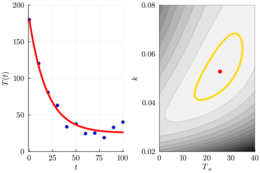
Figure 1: Left panel: synthetic data (blue dots) showing observations $T^{\textrm{o}}(t)$ at $t=0,10,20,\ldots,100$ superimposed with the MLE solution (solid red) with $\hat{\theta}=(\hat{T_{a}},\hat{k})^{\mathsf{T}}=(25.386,0.053)^{\mathsf{T}}$. Right panel: heat map of $\bar{\ell}(\theta\mid T^{\textrm{o}}(t))$ superimposed with the MLE (red dot) and a contour at $\bar{\ell}^{*}=-\Delta_{0.95,2}/2\approx-2.996$ (solid gold). The greyscale shading darkens with decreasing $\bar{\ell}$. Data in the left panel are obtained by solving (1) with $\theta=(20,0.05)^{\mathsf{T}}$ and corrupting the solution at $t=0,10,20,\ldots,100$ with additive Gaussian noise with $\sigma=8$. The units of temperature are ^∘C; time is measured in minutes; and the dimensions of $k$ are /minute.

This imperfect, noisy data motivates us to ask four natural questions:

1. What value of $\theta=(T_{a},k)^{\mathsf{T}}$ in (1) gives $T(t)$ that provides the best match to the data?

2. How confident are we in these best-fit estimates of $\theta$? In other words, to what extent does the imperfect data constrain our estimate of $\theta$?

3. How do we measure uncertainty in our estimate of $\theta$?

4. How does variability in $\theta$ translate into prediction variability when we consider using (1) to predict the temporal evolution of $T(t)$?

We will illustrate a relatively simple approach to address these questions using standard computational tools, with the most advanced concept that we rely on relating to numerical optimization [6].

In this context we will refer to Newton’s law of cooling, (1), as a process model because this mathematical model describes the process of interest (i.e. heat transfer). To proceed we also introduce a noise model which relates the observed data $T^{o}(t)$ to the solution of the process model $T(t)$. In this first example we make a standard assumption that the observed data, $T^{\textrm{o}}(t)$, can be interpreted as samples from a normal distribution where the mean of that distribution is the solution of the process model. Under this standard approach, at any time $t$ we have $T^{\textrm{o}}(t)\mid\theta\sim\mathcal{N}\left(T(t),\sigma^{2}\right)$, where $T(t)$ is the solution of (1) at time $t$, and $\sigma^{2}$ is a constant variance. This noise model gives us a straightforward way of relating the solution of the process model to the observed data through the probability density function of the normal distribution. For example, suppose we have measured some value of $T^{\textrm{o}}(\tau)$ at time $t=\tau$. Within this framework we can compute the density of various predictions using properties of the normal distribution since we have $T^{\textrm{o}}(\tau)~{}\mid~{}\theta~{}\sim~{}\mathcal{N}\left(T(\tau),\sigma^{2}\right)$. In the simple case of having a single measurement it is clear that the value of $T(\tau)$ that best matches the single measurement is $T(\tau)=T^{\textrm{o}}(\tau)$. If $T(\tau)\neq T^{\textrm{o}}(\tau)$, we can quantify this in a probabilistic sense in terms of the probability density function.

For a series of measurements at time $t_{i}$ for $i=1,2,3,\ldots,I$, it is unreasonable to expect that the solution of the process model will perfectly match all observations simultaneously. One way of interpreting the noise model is that it represents independent fluctuations in the data. Therefore, invoking an independence assumption means that we can evaluate the probability density at each of the $I$ measurements since $T^{\textrm{o}}(t_{i})\mid\theta\sim\mathcal{N}\left(T(t_{i}),\sigma^{2}\right)$, and taking the product of these probability densities gives us a quantity, called the likelihood, which describes the joint probability density of the observed data. As we might anticipate, taking a product like this can lead to extremely small numerical quantities which can be circumvented by taking logarithms, giving rise to the log-likelihood which can be written as

$$\ell(\theta\mid T^{\textrm{o}}(t))=\sum_{i=1}^{I}\log\left[\phi\left(T^{\textrm{o}}(t_{i});T(t_{i}),\sigma^{2}\right)\right],$$ (2)

where $\phi(x;\mu,\sigma^{2})$ denotes the probability density function of the normal distribution with mean $\mu$, variance $\sigma^{2}$, and $T(t_{i})$ is the solution of (1) at time $t=t_{i}$ for $i=1,2,3,\ldots,I$. In the case of working with an additive Gaussian noise model with constant $\sigma$ we can re-write the right of (3) to show that the log-likelihood is related to a sum of squares objective function [2].

Given the log-likelihood function we may now address the first question (above) using numerical optimization to estimate the value of $\theta$, denoted $\hat{\theta}$, that maximises the log-likelihood, $\sup_{\theta}\ell(\theta\mid T^{\textrm{o}}(t))$. For simple problems with one or two unknown parameters we can visualize this maximization simply by plotting $\ell(\theta\mid T^{\textrm{o}}(t))$ as a function of $\theta$ and visually identifying the value of $\theta$ that maximizes $\ell(\theta\mid T^{\textrm{o}}(t))$. For more complicated problems, with three or more unknown values, this graphical approach is infeasible so we use numerical optimisation. All numerical optimization results in this work use the NLopt routine [7] where the Nelder-Mead algorithm is implemented with simple bound constraints. Figure 1 shows a filled greyscale contour plot of $\ell((T_{\textrm{a}},k)^{\mathsf{T}}\mid T^{\textrm{o}}(t))$ where we see that a single value of $\theta$ maximizes the log-likelihood function. In this case numerical optimization gives $\hat{\theta}=(25.386,0.053)^{\mathsf{T}}$ which is the maximum likelihood estimate (MLE). Evaluating (1) at the MLE, and superimposing the MLE solution onto the data in Figure 1 indicates that this solution provides a good visual match to the data.

Our point estimate of $\hat{\theta}$ gives us the value of $\theta$ that means that $T(t)$ is the best match to the data, but this point estimate does not provide any indication of uncertainty in our estimate of $\theta$. To address our second question (above) we will work with the normalised log-likelihood function

$$\bar{\ell}(\theta\mid T^{\textrm{o}}(t))=\ell(\theta\mid T^{\textrm{o}}(t))-\ell(\hat{\theta}\mid T^{\textrm{o}}(t)),$$ (3)

so that we have $\bar{\ell}(\hat{\theta}\mid T^{\textrm{o}}(t))=0$.

The key to inferential precision is the curvature of the log-likelihood function. Intuitively we expect that if $\bar{\ell}(\theta\mid T^{\textrm{o}}(t))$ is tightly peaked near $\hat{\theta}$ then the data constrains our parameter estimates to a relatively narrow region in parameter space. In contrast, if $\bar{\ell}(\theta\mid T^{\textrm{o}}(t))$ is relatively flat near $\hat{\theta}$ then the data contains insufficient information to constrain our estimate of $\theta$ and it is possible that the solution of the model with many values of $\theta$ can accurately match the data.

The degree of curvature of the log-likelihood function can be graphically assessed for mathematical models involving just one or two parameters, but more generally we use numerical optimization together with the concept of the profile likelihood [8] to provide insight where simple visualization is not possible for higher dimensional problems.

To assess the identifiability of each parameter in a model we construct a series of univariate profile likelihood functions. Profile likelihood functions have a simple interpretation that can be explained in terms of the two-dimensional contour plots of the log-likelihood function in Figure 1. First, we will focus our attention on $T_{a}$ by considering a uniform discretisation of that parameter across an interval of interest, for example $T_{a}=0,1,2,\ldots,40$^∘C. For each fixed value of $T_{a}$ along the discretisation, denoted $T_{a}^{\dagger}$, we consider the value of $\bar{\ell}$ along the vertical line at the fixed value of $T_{a}=T_{a}^{\dagger}$. Along this vertical line we identify the value of $k$ that maximises $\bar{\ell}$. This optimization process can be visualized using the heat map of $\bar{\ell}$ in Figure 1. Repeating this optimization for each value of $T_{a}$ over a uniform grid reduces the two-dimensional log-likelihood function to a univariate function, called the profile likelihood [8], which we denote $\bar{\ell}_{p}$. This univariate profile likelihood function can be used qualitatively and quantitatively to assess the curvature of the log-likelihood function at the MLE.

This process of holding one interest parameter constant and optimising out the remaining nuisance parameters by maximising the log-likelihood function can be repeated for all components of $\theta$. In Figure 1 we only have two parameters so we have two univariate profile likelihood functions. We can obtain the second profile likelihood by treating $k$ as the interest parameter across a uniform disretisation $k=0.02,0.025,0.03,\ldots,0.10$ /minute, and for each value of $k$ along the uniform discretisation, $k^{\dagger}$, we identify the value of $T_{a}$ that maximises $\bar{\ell}$ along the horizontal line where $k=k^{\dagger}$. Repeating this process for all values of $k$ along the uniform discretisation of $k$ generates a univariate profile likelihood function for the interest parameter $k$.

For our simple problem with two unknown parameters the process of fixing one interest parameter and optimising out the other nuisance parameter has a simple graphical interpretation that is unclear for higher dimensional problems with three or more parameters. Therefore, in general we use numerical optimization to construct univariate profile likelihood functions since this approach can be used regardless of the number of unknown parameters. Results in Figure 2 show the univariate profile likelihood functions for $T_{a}$ and $k$ obtained using the same numerical optimisation algorithm that we used to estimate the MLE. Both univariate profile likelihood functions involve a single, well-defined peak at the MLE indicating that these parameters are identifiable.

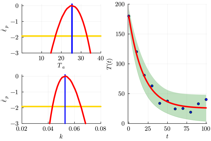
Figure 2: Left panel: Univariate profile likelihood functions for $T_{a}$ and $k$, as indicated (solid red). Each profile indicates the MLE (solid blue) and the $95\%$ threshold $\bar{\ell}^{*}=-\Delta_{0.95,1}/2\approx-1.921$ contour (solid gold). The 95% confidence intervals are $T_{a}\in[16.977,32.983]$ and $k\in[0.0432,0.0648]$. Right panel shows the data (blue dots), MLE solution (red dots) and a 95% prediction interval (green shaded region). The units of temperature are ^∘C; time is measured in minutes; and the dimensions of $k$ are /minute.

The degree of curvature of the log-likelihood function can be quantified in several ways. In this work we take a very simple approach by identifying a threshold–based interval for each parameter defined by defined by the interval where the $\bar{\ell}_{p}\geq\bar{\ell}^{*}$, where the threshold log-likelihood value is associated with an asymptotic confidence interval [9]. The threshold profile log-likelihood value can be approximately calibrated using the $\chi^{2}$ distribution, leading to $\bar{\ell}^{*}=-\Delta_{n,q}/2$ where $\Delta_{n,q}$ refers to the $q$th quantile of a $\chi^{2}$ distribution with $n$ degrees of freedom, taken to be the dimension of the parameter of interest (i.e. the number of interest parameters) [9]. For example, with the univariate profile likelihood functions (where the dimension of the interest parameter is one) we can identify a 95% confidence interval with the threshold of $\bar{\ell}^{*}=-\Delta_{1,0.95}/2\approx-1.9121$. For $T_{a}$, the MLE is $\hat{T_{a}}=25.386$ ^∘C, and the 95% confidence interval is $T_{a}\in[16.977,32.983]$ ^∘C.

Results in Figures 1–2 have answered the first three of four questions (above), confirming that we can estimate the best-fit parameters, and establish our uncertainty in these estimates. We now turn to examining how our uncertainty in $\theta$ can be related to the predictive uncertainty in $T(t)$. The log-likelihood function in Figure 1 is superimposed with a contour at threshold value $\bar{\ell}^{*}=-\Delta_{2,0.95}/2\approx-2.9957$. Choices of $\theta$ within this contour are contained within the asymptotic 95% confidence set of $\theta$ whereas choices outside of this contour are not.

To explore how variability of $\theta$ within this confidence set translates into variability in predictions of $T(t)$ we can randomly sample values of $\theta=(T_{a},k)^{\mathsf{T}}$ to generate a set of $M$ samples within the confidence set. For each of the $M$ samples we evaluate (1) to give $M$ solution curves, $T_{m}(t)$ for $m=1,2,3,\ldots,M$. According to the noise model, these $M$ solutions describe the curvewise mean of the noise model distribution. To provide a measure of the variability about each mean trajectory we can use properties of our noise model to quantify and visualise the variability in $T(t)$ about the mean. A standard way to characterize the width of a probability distribution is to consider various quantiles of that distribution. For example, the 20% and 80% quantiles of the $\mathcal{N}(0,1)$ distribution are approximately $\pm 0.8416$, whereas the 5% and 95% quantiles are approximately $\pm 1.645$.

Using these ideas we describe the variability about the mean trajectories noting that with $\sigma=8$ the 5% and 95% quantiles define a curve-wise interval $T_{m}(t)\pm 13.159$ for each trajectory $m=1,2,3,\ldots,M$. To provide an overall prediction interval that accounts for variability associated with the noise model and the variability introduced by considering different choices of $\theta$ within the confidence set we evaluate $T_{m}(t)$ at $t=0,1,2,3,\ldots,100$ minutes for each of the $M$ trajectories. We than record the maximum and minimum values of of $T_{m}(t)\pm 13.159$ across all $M$ trajectories evaluated at $t=0,1,2,3,\ldots,100$ minutes to give the prediction interval in Figure 2. This prediction interval provides a quantitative indication of how variability in $\theta$ maps to variability in $T(t)$. The prediction interval in Figure 2 is obtained using $M=1000$ samples. In this case this choice of $M$ is sufficiently large that the prediction interval is insensitive to taking more samples of $\theta$.

3 Modeling with PDEs

This example we will demonstrate how the concepts developed in Section 2 can be adapted to apply to mathematical models based on PDEs by working with the advection-diffusion equation to describe the spatio-temporal distribution of a non-dimensional concentration $u(x,t)\geq 0$,

$$\dfrac{\partial u}{\partial t}=D\dfrac{\partial^{2}u}{\partial x^{2}}-v\dfrac{\partial u}{\partial x},\quad\textrm{on}\quad-\infty<x<\infty,$$ (4)

where $D>0$ [L²/T] is the diffusion coefficient, and $v$ [L/T] is the advective velocity. This mathematical model is widely used in various physical, chemical and biological applications, such as the study of the dispersion of dissolved solutes (e.g. nutrients, pollutants) in porous media [10]. We will consider the solution of (4) for the initial condition $u(x,0)=u_{b}+u_{0}$ for $x<|h|$, and $u(x,0)=u_{b}$ for $x>|h|$. We interpret $u_{b}\geq 0$ as a uniform background concentration of $u$, and we are particularly interested in the spatial spreading of $u$ that arises when an additional amount of $u$ is placed uniformly within distance $h>0$ from the origin, giving $u(x,0)=u_{b}+u_{0}$ for $x<|h|$, where $u_{0}>0$. This initial condition is plotted in Figure 3 where we have a background concentration $u_{b}=1$, and locally within the interval $-50<x<50$ we have $u(x,0)=2$. The solution of the mathematical model describes how this additional solute within $-50<x<50$ undergoes combined advection and diffusive transport as a function of position $x$ and time $t$.

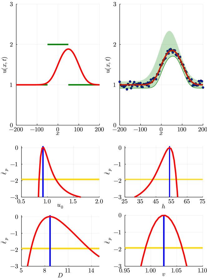
Figure 3: Upper left panel: initial condition $u(x,0)$ (solid green) with $u_{b}=u_{0}=1$ and $h=50$ superimposed with the PDE solution at $t=50$, $u(x,50)$ (solid red) with $D=10$ and $v=1$. Upper right panel: synthetic data (blue dots) showing observations $u^{\textrm{o}}(x,50)$ at $x=-200,-195,-190,\ldots,195,200$ superimposed with the MLE solution (solid red) with $\hat{\theta}=(\hat{u_{0}},\hat{h},\hat{D},\hat{v})^{\mathsf{T}}=(0.914,53.693,8.671,1.025)^{\mathsf{T}}$ and the 95% prediction interval (green shaded region). The data is obtained by evaluating (4) with $(u_{0},h,D,v)^{\mathsf{T}}=(1,50,10,1)^{\mathsf{T}}$ at $x=-200,-195,-190,\ldots,195,200$ and corrupting each data point with additive Gaussian noise with $\sigma=0.05$. Bottom panels: profile likelihood functions $u_{0}$, $h$, $D$ and $v$, as indicated (solid red). Each profile indicates the MLE (solid blue) and the $95\%$ threshold $\bar{\ell}^{*}=-\Delta_{0.95,1}/2\approx-1.921$ (solid gold). The 95% confidence intervals are $u_{0}\in[0.839,1.156]$, $h\in[42.939,58.043]$, $D\in[6.227,13.686]$ and $v\in[0.990,1.060]$.

The solution of (4) with these initial conditions can be obtained using a Fourier transform and is given by

$$u(x,t)=u_{b}+\dfrac{u_{0}}{2}\left[\textrm{erf}\left(\dfrac{h-(x-vt)}{2\sqrt{Dt}}\right)+\textrm{erf}\left(\dfrac{h+(x-vt)}{2\sqrt{Dt}}\right)\right],$$ (5)

where $\textrm{erf}(x)=\left(2/\sqrt{\pi}\right)\int_{0}^{x}\textrm{exp}(-z^{2})\;\textrm{d}z$ is the error function [11]. Results in Figure 3 superimpose the exact solution for $(u_{0},h,D,v)^{\top}=(1,50,10,1)$ at $t=50$ onto the plot of $u(x,0)$ and we see that the centre of mass of $u(x,50)$ translates in the positive $x$-direction from $x=0$ to $x=50$ as a result of the advective transport. In addition, the discontinuous $u(x,0)$ profile becomes continuous and smooth by $t=50$ owing to the action of diffusive transport.

Discrete data, shown in Figure 3, is obtained by evaluating the exact solution, $u(x,50)$ at $x=-200,-195,-190,\ldots,200$ and then corrupting each value of $u(x,50)$ with additive Gaussian noise with $\sigma=0.05$. Given this noisy data we will now address the same questions of parameter estimation, parameter identifiability and model prediction as in Section 2 except now we are dealing with four parameters $\theta=(u_{0},h,D,v)^{\mathsf{T}}$ in the PDE model. An important consequence of working with a larger number of unknown parameters is that we can no longer simply visualize the log-likelihood function as we did in Figure 1.

As in the ODE model, here we have a log-likelihood function

$$\ell(\theta\mid u^{\textrm{o}}(x_{i},t))=\sum_{i=1}^{I}\log\left[\phi\left(u^{\textrm{o}}(x_{i},t);u(x_{i},t),\sigma^{2}\right)\right],$$ (6)

where again $\phi(x;\mu,\sigma^{2})$ denotes the probability density function of the normal distribution with mean $\mu$, variance $\sigma^{2}$. Here, the index $i$ refers to the spatial position where measurements are taken. Although we are unable to visualize this function like we did in Section 2, numerical optimization gives $\hat{\theta}=(0.914,53.693,8.671,1.025)^{\mathsf{T}}$. Superimposing $u(x,t)$ evaluated with $\hat{\theta}$ in Figure 3 indicates that the solution provides a good visual match to the data, as anticipated. Given the MLE we can now work with a normalized log-likelihood function

$$\bar{\ell}(\theta\mid u^{\textrm{o}}(x,t))=\ell(\theta\mid u^{\textrm{o}}(x,t))-\ell(\hat{\theta}\mid u^{\textrm{o}}(x,t)),$$ (7)

which can be used to construct various profile likelihood functions to explore the identifiability of the four parameters. Since we have four unknown parameters we construct four univariate profile likelihood functions and the approach for each is the same. For example, if we take $u_{0}$ to be the interest parameter and $(h,D,v)^{\mathsf{T}}$ to be the nuisance parameters, the profile likelihood for $u_{0}$ can be written as

$$\bar{\ell}_{p}(u_{0}\mid u^{\textrm{o}}(x,t))=\sup_{(h,D,v)^{\mathsf{T}}}\bar{\ell}(\theta\mid u^{\textrm{o}}(x,t)),$$ (8)

which can be evaluated by holding $u_{0}$ at some fixed value $u_{0}^{\dagger}$ and computing values of $(h,D,v)^{\mathsf{T}}$ that maximise $\bar{\ell}$ using numerical optimization. Repeating this process across a grid of $u_{0}$ gives a univariate profile likelihood as shown in Figure 3 where we see that the univariate profile likelihood for $u_{0}$ has a single peak at the MLE, $\hat{u}_{0}=0.914$, and approximate 95% confidence intervals are $u_{0}\in[0.839,1.156]$. Repeating this process to construct univariate profile likelihood functions for $h$, $D$ and $v$ leads to the profile likelihood functions given in Figure 3 indicating that all parameters are practically identifiable in this case.

We conclude this exercise by returning to the full log-likelihood function and using rejection sampling to generate $M$ parameter samples $\theta$, where $\bar{\ell}\geq\bar{\ell}^{*}$. Evaluating $u(x,t)$ for each of the $M$ parameter samples, computing the 5% and 95% quantiles of the noise model at each value of $x$, and then evaluating the maximum and minimum at $x=-200,-195,-190,\ldots,200$ over all $M$ samples gives the prediction interval in Figure 3 which illustrates how parameter estimates within the 95% confidence set translate into a prediction interval in $u(x,50)$ for this problem.

This PDE example highlights a serious shortcoming of working with the additive Gaussian noise model. A mathematical property of the exact solution, (5) is that $u_{b}<u(x,t)<u_{0}+u_{b}$ for $t>0$. Our data in Figure 3 clearly violates this property as we have $u^{\textrm{o}}<u_{b}$ at several locations. This issue is even more concerning if we consider the realistic case of having no background concentration by setting $u_{b}=0$. Under these circumstances working with additive Gaussian noise is clearly unsatisfactory since this leads to $u<0$ which is physically impossible.

One way to address this shortcoming is to implement a different noise model. In this case we could instead introduce a multiplicative noise model where $u^{\textrm{o}}(x_{i},t)\mid\theta=(u(x_{i},t)\mid\theta)\eta_{i}$ where $\eta_{i}\sim\textrm{Log-normal}(0,\sigma^{2})$ [12]. Our previous examples with additive Gaussian noise models have a constant variability whereas the multiplicative log-normal noise model has variability that increases with $u^{\textrm{o}}(x,t)$. The Log-normal noise model also has the attractive property that the variability vanishes as $u^{\textrm{o}}(x,t)~{}\to~{}0^{+}$. Figure 4 shows a solution of (4) with $u_{b}=0$ and $(u_{0},h,D,v)^{\mathsf{T}}=(1,50,10,1)^{\mathsf{T}}$ at $t=50$, where the solution at $x=-200,-195,-190,\ldots,200$ is corrupted with multiplicative log-normal noise with $\sigma=0.2$. Here we see that the data is noise-free as $u\to 0^{+}$ and the variability is largest near $x=50$ where $u(x,t)$ is a maximum at this time.

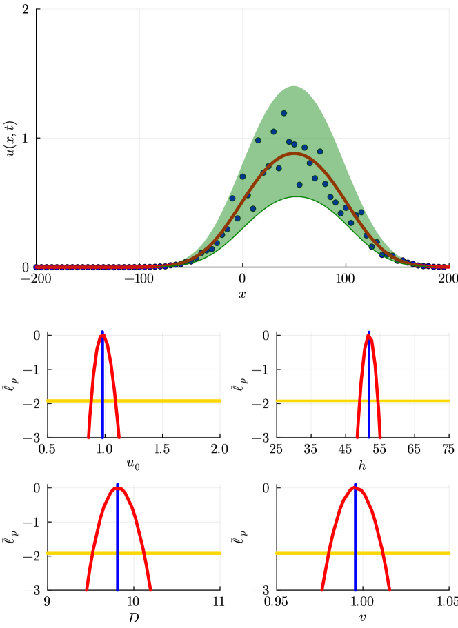
Figure 4: Upper panel: synthetic data (blue dots) that represent observations $u^{\textrm{o}}(x,50)$ at $x=-200,-195,-190,\ldots,195,200$ superimposed on the MLE solution (solid red) with $\hat{\theta}=(\hat{u_{0}},\hat{h},\hat{D},\hat{v})^{\mathsf{T}}=(0.977,51.776,9.813,0.996)^{\mathsf{T}}$ and a 95% prediction interval (green shaded region). The data is obtained by evaluating (5) with $(u_{0},h,D,v)^{\mathsf{T}}=(1,50,10,1)^{\mathsf{T}}$ at $x=-200,-195,-190,\ldots,195,200$ and corrupting each value of $u$ with with multiplicative log-normal noise with $\sigma=0.2$. Bottom panels: profile likelihood functions $u_{0}$, $h$, $D$ and $v$, as indicated (solid red). Each profile indicates the MLE (solid blue) and the $95\%$ threshold $\bar{\ell}^{*}=-\Delta_{0.95,1}/2\approx-1.921$ (solid gold). The 95% confidence intervals are $u_{0}\in[0.879,1.090]$, $h\in[49.064,54.380]$, $D\in[9.522,10.117]$ and $v\in[0.980,1.012]$.

For the multiplicative log-normal noise model framework we have a log-likelihood function of the form

$$\ell(\theta\mid u^{\textrm{o}}(x_{i},t))=\sum_{i=1}^{I}\log\left[\phi\left(u^{\textrm{o}}(x_{i},t);\log(u(x_{i},t)),\sigma^{2}\right)\right],$$ (9)

where $\phi(x;\mu,\sigma)$ is the probability density function of the Log-normal$(\mu,\sigma^{2})$ distribution. Maximising this log-likelihood function gives $\hat{\theta}=(0.977,51.776,9.813,0.996)^{\mathsf{T}}$, and superimposing $u(x,t)$ evaluated with $\hat{\theta}$ in Figure 4 indicates that the solution matches the data reasonably well.

Given our log-likelihood function and our estimate of $\hat{\theta}$, we can work with a normalised log-likelihood function and repeat the construction of the four univariate profile likelihood functions in exactly the same way as we did for the additive Gaussian noise model. The univariate profile likelihood functions in Figure 4 indicate that the four parameters are practically identifiable. As before, we can sample the log-likelihood function to obtain $M$ parameter samples $\theta$ with $\bar{\ell}\geq\bar{\ell}^{*}$ and use these $M$ solutions of (4) to construct the 95% prediction interval given in Figure 4. For the multiplicative noise model we see that the prediction intervals have the attractive property that the upper and lower bounds are always non-negative. This is very different to working with an additive Gaussian noise model since this procedure can lead to negative prediction intervals which is not physically realistic.

4 Modeling with a BVP: Dealing with non-identifiability

In this section we will work with a linear BVP that illustrates how non-identifiability can arise, even in very simple mathematical models. We consider a simple reaction-diffusion equation that has often been used as a caricature model of the morphogen gradients that arise during embryonic development and are thought to be associated with spatial patterning during morphogenesis [13]

$$\dfrac{\partial u}{\partial t}=D\dfrac{\partial^{2}u}{\partial x^{2}}-ku,\quad\textrm{on}\quad x>0,$$ (10)

where $u(x,t)$ represents a non-dimensional morphogen concentration at location $x$ at time $t$. This model is often considered with the trivial initial condition $u(x,0)=0$. The morphogen gradient is formed along the $x$-axis by a constant diffusive flux in the positive $x$-direction applied at the origin $J=-D\partial u/\partial x$ at $x=0$. This simple model assumes that the morphogens undergo diffusion with diffusivity $D>0$ [L²/T], as well as undergoing some decay process that is modelled with a first-order decay term with decay rate $k>0$ [/T]. The mathematical model is closed by assuming that the solution vanishes in the far field, that is $u\to 0$ as $x\to\infty$.

While, in principal, it is possible to use an integral transform to solve (10) to give an expression for $u(x,t)$ like we did in Section 3 for the advection-diffusion equation, it is both mathematically convenient and biologically relevant to consider the long-time limit of the time-dependent solution by studying the steady-state distribution, $\displaystyle{\lim_{t\to\infty}}u(x,t)=U(x)$, where $U(x)$ is governed by the following BVP,

$$0=D\dfrac{\textrm{d}^{2}U}{\textrm{d}x^{2}}-kU,\quad\textrm{on}\quad x>0,$$ (11)

with $\textrm{d}U/\textrm{d}x=-J/D$ at $x=0$, and $U\to 0$ as $x\to\infty$. The solution of the steady state BVP can be written

$$U=\dfrac{J}{\sqrt{Dk}}\textrm{exp}\left(-x\sqrt{\dfrac{k}{D}}\right).$$ (12)

As for the PDE model in Section 3, here we have $U>0$ by definition. Accordingly, we present data in Figure 5 corresponding to $\theta=(J,D,k)^{\mathsf{T}}=(1,1,0.1)^{\mathsf{T}}$ on the truncated domain $0<x<20$. The solution at $x=0,2,4,\ldots,20$ is corrupted with multiplicative log-normal noise with $\sigma=0.5$ and, as expected, we see the fluctuations in the data vanish as $x\to\infty$ where $U\to 0^{+}$. With this framework we have a log-likelihood function of the form

$$\ell(\theta\mid U^{\textrm{o}}(x_{i}))=\sum_{i=1}^{I}\log\left[\phi\left(U^{\textrm{o}}(x_{i});\log(U(x_{i})),\sigma^{2}\right)\right],$$ (13)

where $\phi(x;\mu,\sigma)$ is the probability density function of the Log-normal$(\mu,\sigma^{2})$ distribution. Numerical optimization gives $\hat{\theta}=(\hat{J},\hat{D},\hat{k})^{\mathsf{T}}=(1.171,1.100,0.108)^{\mathsf{T}}$, and superimposing $U(x)$ evaluated at $\hat{\theta}$ on the data indicates that the solution provides a good match to the data, but as with all previous problems the MLE point estimate provides no insight into parameter identifiability. The identifiability can be assessed using the exact same procedures implemented in Section 3 to give the univariate profiles for $J$, $D$ and $k$ in Figure 5. These univariate profile likelihood functions immediately indicate that these parameters are not well identified by this data because the profiles are flat. The flat profiles indicate that there are many different parameter choices for which (12) matches the data equally well, which is an example of non-identifiability [14, 2, 15, 16].

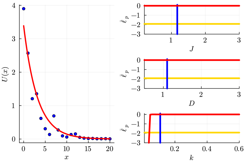
Figure 5: Left panel: synthetic data (blue dots) showing observations $U^{\textrm{o}}(x)$ at $x=0,2,4,\ldots,20$ superimposed with the MLE solution (solid red) with $\hat{\theta}=(\hat{J},\hat{D},\hat{k})^{\mathsf{T}}=(1.171,1.100,0.108)^{\mathsf{T}}$. Right panel: Profile likelihood functions for $J$, $D$ and $k$, as indicated (solid red). Each profile indicates the MLE (solid blue) and the $95\%$ threshold $\bar{\ell}^{*}=-\Delta_{0.95,1}/2\approx-1.921$ (solid gold). The data is obtained by solving (11) with $\hat{\theta}=(1,1,0.1)$ and corrupting the solution at $x=0,2,4,\ldots,20$ with multiplicative log-normal noise with $\sigma=0.5$.

In this particular example, the mathematical structure of the solution of the model, (12), indicates that the parameters are not identifiable because as $U(x)$ depends upon a particular combination of parameters, namely $J/\sqrt{kD}$ and $\sqrt{k/D}$. Since there are infinitely many choices of $J,D$ and $k$ that lead to identical combinations of $J/\sqrt{kD}$ and $\sqrt{k/D}$ it is not surprising that the profile likelihood functions in Figure 5 are flat.

In this case the structure of the exact solution suggests that a re-parameterisation of the likelihood function is possible, $\theta=(\alpha,\beta)^{\mathsf{T}}$, where $\alpha=J/\sqrt{kD}$ and $\beta=\sqrt{k/D}$, so that we may attempt to estimate $\theta=(\alpha,\beta)^{\mathsf{T}}$ instead of estimating $\theta=(J,D,k)^{\mathsf{T}}$. Results in Figure 6 re-examine the same set of data using the re-parameterised log-likelihood function, and numerical optimization gives $\hat{\theta}=(3.389,0.3141)^{\mathsf{T}}$. We can examine the identifiability of the re-scaled parameters by constructing univariate profile likelihood functions for $\alpha=J/\sqrt{kD}$ and $\beta=\sqrt{k/D}$ where we find that both quantities are well identified by the data. Repeating the process of sampling $M$ values of $\theta=(\alpha,\beta)^{\mathsf{T}}$ where $\bar{\ell}\geq\bar{\ell}^{*}$ and using these $M$ solutions of (11) to construct the 95% prediction interval given in Figure 6 where we again see that the prediction intervals have the useful property that they are non-negative.

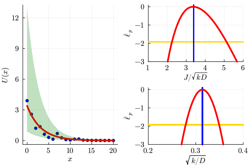
Figure 6: Left panel: synthetic data (blue dots) showing observations $U^{\textrm{o}}(x)$ at $x=0,2,4,\ldots,20$ superimposed with the MLE solution (solid red) with $\hat{\theta}=(\hat{\alpha},\hat{\beta})^{\mathsf{T}}=(3.389,0.3141)^{\mathsf{T}}$ and the 95% prediction interval (shaded green region). Right panel: profile likelihood functions for $\alpha=J/\sqrt{kD}$ and $\beta=\sqrt{k/D}$, as indicated (solid red). Each profile indicates the MLE (solid blue) and the $95\%$ threshold $\hat{\ell}^{*}=-\Delta_{0.95,1}/2\approx-1.921$ (solid gold). The 95% confidence intervals are $\alpha=J/\sqrt{kD}\in[2.243,5.121]$, $\beta=\sqrt{k/D}\in[0.279,0.349]$. The data is obtained by solving (11) with $\hat{\theta}=(1,1,0.1)$ and corrupting the solution at $x=0,2,4,\ldots,20$ with multiplicative log-normal noise with $\sigma=0.5$.

5 Extensions and general remarks

This article describes a set of self-contained computational exercises that develop awareness, knowledge and skills relating to parameter estimation, parameter identifiability and model prediction. A key aim of these exercises is to illustrate how a likelihood-based approach can be applied to a range of different process models that are of interest to applied mathematicians (e.g. ODE, PDE, BVP-based models). Details of all computational exercises can be repeated and extended using open source software available on GitHub.

The example problems dealt within this article reflect a compromise between keeping all calculations sufficiently straightforward while also working with mathematical modelling scenarios of practical interest. Accordingly there are many ways that the examples can be extended. For example, all data considered in this article are generated using either an additive Gaussian noise model or a multiplicative Log-normal noise model with a known variance. While sometimes it is possible to pre-estimate the value of $\sigma$ from a real data set, it is also straightforward to extend the vector of unknown parameters and treat $\sigma$ as an unknown quantity to be determined along with the other model parameters. Similarly, when we dealt with the PDE model in Section 3 we considered data at several spatial locations, $u^{\textrm{o}}(x_{i},t)$ for $i=1,2,3,\ldots,I$, but just one fixed point in time. In many situations data are available at different points in space and at different times, $u^{\textrm{o}}(x_{i},t_{j})$ for $i=1,2,3,\ldots,I$ and $j=1,2,3,\ldots,J$, and dealing with such data is straightforward by summing over all data points, both in space and time, in the log-likelihood function, (9).

Another common feature of the examples presented in this article is that we have chosen to work with process models that take the form of analytically tractable differential equations. In general, our ability to work with analytically tractable models is usually limited to special cases, such as dealing with linear differential equations. Therefore, another useful extension of the exercises presented here is to replace the use of the exact solutions with a numerical solution, obtained for example using the DifferentialEquations.jl package in Julia to solve time-dependent ODE models [17]. Repeating the exercises in this article using numerical solutions will be a useful stepping-stone for readers who are interested in using more general process models based on nonlinear differential equations where exact solutions are not always possible.

In terms of making model predictions, we always used a very simple rejection sampling method to find $M$ samples of $\theta$ where the log-likelihood function is great than some asymptotic threshold. We chose to use rejection sampling because it is both simple to implement and interpret, but other approaches are possible. For example, we could have simply used a uniform discretisation of the log-likelihood function and evaluated $\bar{\ell}$ across a uniform mesh to propagate the parameter confidence set through to examine model predictions. Both approaches carry advantages and disadvantages and give very similar results provided that $M$ is chosen to be sufficiently large when using rejection sampling, and that the uniform mesh is taken to be sufficiently dense when working with a gridded log-likelihood function.

Our results in Section 4 demonstrate how non-identifiability manifests as flat univariate profile likelihood functions, and in this case we are able to use the exact solution of the BVP to motivate a simple re-parameterization of the log-likelihood function. This approach, while instructive, is not always possible when the process model is intractable. In such cases it is sometimes possible to use different methods to determine appropriate re-parameterization options [1].

A key feature of the computational exercises in this work is that in each case we used synthetic data collected from a particular ODE, PDE or BVP model, and then we used the same model for parameter estimation. This is convenient from the point of view of demonstrating and exploring these computational techniques, however in real-world applications there is always some inherent uncertainty in the mechanisms acting to produce experimental data. As such, the question of model selection arises because there is almost always more than one possible process model that can be applied to replicate and interrogate the data. In these cases the tools developed here to explore parameter identifiability, parameter estimation and model prediction can be used across a number of competing models to help in the process of model selection. In this situation it can be useful to compute profile likelihood functions for each parameter in the competing models which can help to rule out working with a model involving non-identifiable parameter when alternative models are available where all parameters are identifiable [18]. Similarly, when dealing with experimental data it can be useful to compute and compare profile likelihood functions using different noise models [19] to guide the selection of an appropriate noise model. A final comment is that all of the exercises presented in this work deal with deterministic mathematical models. It is possible to apply the same ideas to stochastic mathematical models by using, for example, a coarse-grained continuum limit description of the stochastic model [20, 21]

References

- [1] D. Cole “Parameter redundancy and identifiability” CRC Press, 2020
- [2] K.. Hines, T.. Middendorf and R.. Aldrich “Determination of parameter identifiability in nonlinear biophysical models: A Bayesian approach” In Journal of General Physiology 143, 2014, pp. 401 DOI: 10.1085/jgp.201311116
- [3] D.. Bates and D.. Watts “Nonlinear regression analysis and its applications” New Jersey: Wiley, 1988
- [4] D.. Cox “Principles of statistical interence” Cambridge University Press, 2006
- [5] L. Wasserman “All of statistics: A concise course in statistical inference” Springer, 2004
- [6] C. Audet and W. Hare “Derivative-free and blackbox optimization” Springer, 2017
- [7] S.. Johnson “The NLopt module for Julia”, 2018 URL: https://github.com/JuliaOpt/NLopt.jl
- [8] Y. Pawitan “In all likelihood: statistical modelling and inference using likelihood” Oxford University Press, 2001
- [9] P. Royston “Profile likelihood for estimation and confidence intervals” In The Stata Journal 7, 2007, pp. 376–387
- [10] C. Zheng and G.. Bennett “Applied contaminant transport modelling” Wiley, 2002
- [11] M. Abramowitz and I.. Stegun “Handbook of mathematical functions with formulas, graphs, and mathematical tables” Dover Publications, 1964
- [12] R.. Murphy, O.. Maclaren and M.. Simpson “Implementing measurement error models with mechanistic mathematical models in a likelihood-based framework for estimation, identifiability analysis and prediction in the life sciences” In Journal of the Royal Society Interface 21, 2024, pp. 20230402 DOI: 10.1098/rsif.2023.0402
- [13] Anna Kicheva et al. “Kinetics of morphogen gradient formation” In Science 315.5811, 2007, pp. 521–525 DOI: 10.1126/science.1135774
- [14] I Siekmann, J Sneyd and E J Crampin “MCMC can detect nonidentifiable models” In Biophysical Journal 103, 2012, pp. 2275–2286 DOI: https://doi.org/10.1016/j.bpj.2012.10.024
- [15] F. Fröhlich, F.. Theis and J. Hasenauer “Uncertainty analysis for non-identifiable dynamical systems: Profile likelihoods, bootstrapping and more” In International Conference on Computational Methods in Systems Biology, 2014, pp. 61–72
- [16] M.. Simpson and O.. Maclaren “Making predictions using poorly identified mathematical models” In Bulletin of Mathematical Biology 86, 2024, pp. 80 DOI: 10.1007/s11538-024-01294-0
- [17] C Rackauckas and Q Nie “DifferentialEquations.jl – A performant and feature-rich ecosystem for Solving differential equations in Julia” In Journal of Open Research Software 5.15, 2017 DOI: https://doi.org/10.5334/jors.151
- [18] M.. Simpson et al. “Parameter identifiability and model selection for sigmoid population growth models” In Journal of Theoretical Biology 535, 2022, pp. 1100998 DOI: 10.1016/j.jtbi.2021.110998
- [19] M.. Simpson, R.. Murphy and O.. Maclaren “Modelling count data with partial differential equation models in biology” In Journal of Theoretical Biology 580, 2024, pp. 111732 DOI: 10.1016/j.jtbi.2024.111732
- [20] M J Simpson et al. “Profile likelihood analysis for a stochastic model of diffusion in heterogeneous media” In Proceedings of the Royal Society A: Mathematical, Physical and Engineering Sciences 477, 2021, pp. 20210214 DOI: http://doi.org/10.1098/rspa.2021.0214
- [21] D J Warne et al. “Generalised likelihood profiles for models with intractable likelihoods” In Statistics and Computing 34, 2024, pp. 50 DOI: https://doi.org/10.1007/s11222-023-10361-w