From Entanglement to Universality: A Multiparticle Spacetime Algebra Approach to Quantum Computational Gates Revisited

Abstract

Alternative mathematical explorations in quantum computing can be of great scientific interest, especially if they come with penetrating physical insights. In this paper, we present a critical revisitation of our geometric (Clifford) algebras (GAs) application in quantum computing as originally presented in [C. Cafaro and S. Mancini, Adv. Appl. Clifford Algebras 21, 493 (2011)]. Our focus is on testing the usefulness of geometric algebras (GAs) techniques in two applications to quantum computing. First, making use of the geometric algebra of a relativistic configuration space (a.k.a., multiparticle spacetime algebra or MSTA), we offer an explicit algebraic characterization of one- and two-qubit quantum states together with a MSTA description of one- and two-qubit quantum computational gates. In this first application, we devote special attention to the concept of entanglement, focusing on entangled quantum states and two-qubit entangling quantum gates. Second, exploiting the previously mentioned MSTA characterization together with the GA depiction of the Lie algebras $\mathrm{SO}\left(3;\mathbb{R}\right)$ and $\mathrm{SU}\left(2;\mathbb{C}\right)$ depending on the rotor group $\mathrm{Spin}^{+}\left(3,0\right)$ formalism, we focus our attention to the concept of universality in quantum computing by reevaluating Boykin’s proof on the identification of a suitable set of universal quantum gates. At the end of our mathematical exploration, we arrive at two main conclusions. Firstly, the MSTA perspective leads to a powerful conceptual unification between quantum states and quantum operators. More specifically, the complex qubit space and the complex space of unitary operators acting on them merge in a single multivectorial real space. Secondly, the GA viewpoint on rotations based on the rotor group $\mathrm{Spin}^{+}\left(3,0\right)$ carries both conceptual and computational upper hands compared to conventional vectorial and matricial methods.

I Introduction

A universal mathematical language for physics is the so-called Geometric (Clifford) algebra (GA) hestenes ; dl , a language that relies on the mathematical formalism of Clifford algebra. A very partial list of physical applications of GA methods includes the fields of gravity gull ; francis , classical electrodynamics baylis , and massive classical electrodynamics with Dirac’s magnetic monopoles cafaro ; cafaro-ali . In this paper, however, we are interested in the use of GA in quantum information and quantum computation. The inclusion of Clifford algebra and GA in quantum information science (QIS) is quite reasonable, given some physically motivated grounds vlasov ; doran1 . Indeed, any quantum bit, viewed as the fundamental messenger of quantum information and realized in terms of a spin-$1/2$ system, can be considered as a $2\times 2$ matrix with a second column that is empty. Once this link with $2\times 2$ matrices is made, one recalls that any $2\times 2$ matrix can be expressed as a combination of Pauli matrices. These, in turn, represent some GA. Furthermore, any $2\times 2$ unitary transformation as well can be specified by elements of some GA. Motivated by these considerations, the multiparticle geometric algebra formalism was originally employed in Ref. somaroo to provide a first GA-based reformulation of some of the most important operations in quantum computation. In a more unconventional use of GA in quantum computing, suitable GA structures were used to perform quantum-like algorithms without closely considering quantum theory marek1 ; marek2 ; marek3 . Within this less orthodox approach, the geometric product replaces the standard tensor product. Moreover, multivectors interpreted in a geometric fashion by means of bags of shapes are used to specify ordinary quantum entangled states. The GA approach to quantum computing with states, gates, and quantum algorithms as proposed in Refs. marek1 ; marek2 ; marek3 generates novel conceptual elements in the field of QIS. For instance, the microscopic flavor of the quantum computing formalism is lost when described from the point of view of such a GA approach. This loss leads to a sort of non-microworld implementation of quantum computation. This type of implementation is supported by the thesis carried out in Ref. marek3 , where it is stated that there is no fundamentally basic reason why one should assume that quantum computation must be necessarily associated with physical systems characterized the rules of quantum theory marek3 . An extensive technical discussion on the application of GA methods to QIS is presented in Ref. doran1 . However, this discussion lacks a presentation on the fundamentally relevant notion of universality in quantum computing. Despite that fact that the Toffoli and Fredkin three-qubit quantum gates were formulated in terms of GA in Ref. somaroo , the authors did not consider any explicit characterization of one and two-qubit quantum gates. In Ref. mancio11 , Cafaro and Mancini not only presented an explicit GA characterization of one-qubit and two-qubit quantum states together with a GA description of universal sets of quantum gates for quantum computation, they also demonstrated the universality of a specific set of quantum gates in terms of the geometric algebra language.

In this paper, given the recent increasing visibility obtained by our findings reported in Ref. mancio11 as evident from Refs. hild20 ; ed21 ; alves22 ; hild22 ; J22 ; silva23 ; ery23 ; winter23 ; J23 ; J24 ; toffano24 , we present a critical revisitation of our work in Ref. mancio11 . Our overall scope is to emphasize the concepts of entanglement and universality in QIS after offering an instructive GA characterization of both one- and two-qubit quantum states and quantum gates. More specifically, we begin with the essential elements of the multiparticle spacetime algebra (MSTA, the geometric Clifford algebra of a relativistic configuration space lasenby93 ; cd93 ; doran96 ; somaroo99 ). We then use the MSTA to describe one- and two-qubit quantum states including, for instance, the $2$-qubit Bell states that represent maximally entangled quantum states of two qubits. We then extend the application of the MSTA to specify both one-qubit gates (i.e., bit-flip, phase-flip, combined bit and phase flip quantum gates, Hadamard gate, rotation gate, phase gate and $\pi/8$-gate) and two-qubit quantum computational gates (i.e., CNOT, controlled-phase and SWAP quantum gates) NIELSEN . Then, employing this proposed GA description of states and gates along with the GA characterization of the Lie algebras $\mathrm{SO}\left(3\right)$ and $\mathrm{SU}\left(2\right)$ in terms of the rotor group $\mathrm{Spin}^{+}\left(3\text{, }0\right)$ formalism, we revisit from a GA perspective the proof of universality of quantum gates as discussed by Boykin and collaborators in Refs. B99 ; B00 .

The rest of the paper is formally organized as follows. In Section II, we display the essential ingredients of the MSTA formalism necessary to characterize quantum states and elementary gates in quantum computing from a GA viewpoint. In Section III, we offer an explicit GA description of one- and two-qubit quantum states together with a GA representation of one- and two-qubit quantum computational gates. In addition, we concisely discuss in Section III the extension of the MSTA formalism to density matrices for mixed quantum states. In Section IV, we revisit the proof of universality of quantum gates as originally provided by Boykin and collaborators in Refs. B99 ; B00 by making use of the material presented in Sections II and III and, in addition, by exploiting the above-mentioned GA description of the Lie algebras $\mathrm{SO}\left(3\right)$ and $\mathrm{SU}\left(2\right)$ in terms of the rotor group $\mathrm{Spin}^{+}\left(3\text{, }0\right)$ formalism. We present our concluding remarks in Section V. Finally, some technical details on the algebra of physical space $\mathfrak{cl}(3)$ and the spacetime Clifford algebra $\mathfrak{cl}(1,3)$ appear in Appendix A.

II Basics of Multiparticle Spacetime Algebra

In this section, we describe the essentials of the MSTA formalism that is necessary to characterize, from a GA perspective, elementary gates in quantum computing.

In the orthodox context for quantum mechanics, it is usually assumed that the notions of complex space and imaginary unit $i_{\mathbb{C}}$ are essential. Interestingly, employing the geometric Clifford algebra of real $4$-dimensional Minkowski spacetime dl (i.e., the so-called spacetime algebra (STA)), it can be shown that the $i_{\mathbb{C}}$ that appears in the Dirac, Pauli and Schrödinger equations possesses a clear interpretation in terms of rotations in real spacetime david75 . This bouncing between complex and real quantities in quantum mechanics can can be clearly understood once one introduces the so-called multiparticle spacetime algebra (MSTA), that is to say, the geometric algebra of a relativistic configuration space lasenby93 ; cd93 ; doran96 ; somaroo99 . In the traditional description of quantum mechanics, tensor products are employed to construct multiparticle states as well as many of the operators acting on the states themselves. A tensor product is a formal tool for setting apart the Hilbert spaces of different particles in an explicit fashion. GA seeks to explain, from a fundamental viewpoint, the application of the tensor product in nonrelativistic quantum mechanics by means of the underlying space-time geometry cd93 . Within the GA formalism, the geometric product provides a different characterization of the tensor product. Inspired by the effectiveness of the STA formalism in characterizing a single-particle quantum mechanics, the MSTA perspective on multiparticle quantum mechanics in non-relativistic as well as relativistic settings was initially proposed with the expectation that it would also deliver computational and, most of all, interpretational improvements in multiparticle quantum theory cd93 . Conceptual advances are expected to emerge thanks to the peculiar geometric insights furnished by the MSTA formalism. A distinctive aspect of the MSTA is that it requires, for each particle, the existence of a separate copy of both the time dimension and the three spatial dimensions. The MSTA formalism represents a serious attempt to construct a convincing conceptual setting for a multi-time perspective on quantum theory. In conclusion, the primary justification for employing this MSTA formalism is the attempt of enhancing our comprehension of the very important notions of locality and causality in quantum theory. Indeed, exciting utilizations of the MSTA formalism for the revisitation of Holland’s causal interpretation of a system of two spin-$1/2$ particles holland are proposed in Refs. doran96 ; somaroo99 . Inspired by this line of research, we apply here the MSTA formalism to describe qubits, quantum gates, and to revisit the proof of universality in quantum computing as provided by Boykin and collaborators from a GA viewpoint. For some basic details on the algebra of physical space $\mathfrak{cl}(3)$ and the spacetime Clifford algebra $\mathfrak{cl}(1,3)$, we refer to Appendix A. In what follows, we begin with the $n$-qubit spacetime algebra formalism.

II.1 The $n$-Qubit Spacetime Algebra Formalism

The multiparticle spacetime algebra offers an ideal algebraic structure for the characterization of multiparticle states as well as operators acting on them. The MSTA is the geometric algebra of $n$-particle configuration space.  In particular, for relativistic systems, the $n$-particle configuration space is composed of $n$-copies of Minkowski spacetime with each copy being a $1$-particle space. A convenient basis for the MSTA is specified by the set $\left\{\gamma_{\mu}^{a}\right\}$, with $\mu=0$,.., $3$ and $a=1$,.., $n$ identifying the spacetime vector and the particle space, respectively. These basis vectors $\left\{\gamma_{\mu}^{a}\right\}$ fulfill the orthogonality relations $\gamma_{\mu}^{a}\cdot\gamma_{\nu}^{b}=\delta^{ab}\eta_{\mu\nu}$ where $\eta_{\mu\nu}\overset{\text{def}}{=}$ diag$\left(+\text{, }-\text{, }-\text{, }-\right)$. Observe that, because of the orthogonality conditions, vectors from different particle spaces anticommute. Furthermore, since $\dim_{\mathbb{R}}\left[\mathfrak{cl}\left(1\text{, }3\right)\right]^{n}=2^{4n}$, a basis for the entire MSTA possesses $2^{4n}$ degrees of freedom. In the framework of nonrelativistic quantum mechanics, a single absolute time is used to identify all of the individual time coordinates. One can pick this vector to be $\gamma_{0}^{a}$ for each $a$. Then, bivectors are used for modelling spatial vectors relative to these timelike vectors $\left\{\gamma_{0}^{a}\right\}$ through a spacetime split. Moreover, a basis set of relative vectors is specified by $\left\{\sigma_{k}^{a}\right\}$ where $\sigma_{k}^{a}\overset{\text{def}}{=}\gamma_{k}^{a}\gamma_{0}^{a}$ with $k=1$,.., $3$ and $a=1$,.., $n$. The basis set $\left\{\sigma_{k}^{a}\right\}$ gives rise, for each particle space, to the GA of relative space $\mathfrak{cl}(3)\cong\mathfrak{cl}^{+}(1$, $3)$. Each particle space possesses a basis set specified by,

$$1\text{, }\left\{\sigma_{k}\right\}\text{, }\left\{i\sigma_{k}\right\}\text{, }i\text{,}$$ (1)

where the volume element $i$ denotes the highest grade multivector known as the pseudoscalar. Neglecting the particle space indices, the pseudoscalar is defined as $i\overset{\text{def}}{=}\sigma_{1}\sigma_{2}\sigma_{3}$. The basis set in Eq. (1) characterizes the Pauli algebra, the geometric algebra of the $3$-dimensional Euclidean space dl . However, the three Pauli $\sigma_{k}$ are regarded in GA as three independent basis vectors for real space. They are no longer considered as three matrix-valued components of a single isospace vector. Unlike spacetime basis vectors, note that $\sigma_{k}^{a}\sigma_{j}^{b}=\sigma_{j}^{b}\sigma_{k}^{a}$ for any $a\neq b$. In other words, relative vectors $\left\{\sigma_{k}^{a}\right\}$ originating from distinct particle spaces commute. Observe that the set $\left\{\sigma_{k}^{a}\right\}$ give rise to the space $\left[\mathfrak{cl}(3)\right]^{n}\overset{\text{def}}{=}\mathfrak{cl}(3)\otimes$…$\otimes\mathfrak{cl}(3)$ defined as the direct product space of $n$ copies of $\mathfrak{cl}(3)$, the geometric algebra of the $3$-dimensional Euclidean space. In the context of the MSTA formalism, Pauli spinors can be viewed as elements of the even subalgebra of the Pauli algebra spanned by $\left\{1\text{, }i\sigma_{k}\right\}$ which, in turn, is isomorphic to the quaternion algebra. This even subalgebra of the Pauli algebra is a $4$-dimensional real space in which an arbitrary even element can be recast as $\psi=a^{0}+a^{k}i\sigma_{k}$, where $a^{0}$ and $a^{k}$ are real scalars for any $k=1$, $2$, $3$. A quantum state in ordinary quantum mechanics can be specified by a pair of complex numbers $\alpha$ and $\beta$ as,

$$\left|\psi\right\rangle=\left(\begin{array}[c]{c}\alpha\\ \beta\end{array}\right)=\left(\begin{array}[c]{c}\operatorname{Re}\alpha+i_{\mathbb{C}}\operatorname{Im}\alpha\\ \operatorname{Re}\beta+i_{\mathbb{C}}\operatorname{Im}\beta\end{array}\right)\text{.}$$ (2)

Interestingly, a $1\leftrightarrow 1$ map between Pauli column spinors $\left\{\left|\psi\right\rangle\right\}$ and elements $\left\{\psi\right\}$ of the even subalgebra was shown to be true in Ref. lasenby93 . Indeed, one has

$$\left|\psi\right\rangle=\left(\begin{array}[c]{c}a^{0}+i_{\mathbb{C}}a^{3}\\ -a^{2}+i_{\mathbb{C}}a^{1}\end{array}\right)\leftrightarrow\psi=a^{0}+a^{k}i\sigma_{k}\text{.}$$ (3)

with $a^{0}$ and $a^{k}$ being real coefficients for any $k=1$, $2$, $3$. The set of multivectors $\left\{1\text{, }i\sigma_{1}\text{, }i\sigma_{2}\text{, }i\sigma_{3}\right\}$ denotes the set of computational basis states for the real $4$-dimensional even subalgebra that corresponds to the two-dimensional complex Hilbert space $\mathcal{H}_{2}^{1}$ with standard computational basis specified by $\mathcal{B}_{\mathcal{H}_{2}^{1}}\overset{\text{def}}{=}\left\{\left|0\right\rangle\text{, }\left|1\right\rangle\right\}$. In the context of the GA formalism, the following identifications hold true

$$\left|0\right\rangle\leftrightarrow\psi_{\left|0\right\rangle}^{\left(\text{{GA}}\right)}\overset{\text{def}}{=}1\text{, and }\left|1\right\rangle\leftrightarrow\psi_{\left|1\right\rangle}^{\left(\text{{GA}}\right)}\overset{\text{def}}{=}-i\sigma_{2}\text{.}$$ (4)

Moreover, in GA terms lasenby93 , the action of the usual quantum Pauli operators $\left\{\hat{\Sigma}_{k}\text{, }i_{\mathbb{C}}\hat{I}\right\}$ on the states $\left|\psi\right\rangle$ becomes

$$\hat{\Sigma}_{k}\left|\psi\right\rangle\leftrightarrow\sigma_{k}\psi\sigma_{3}\text{, }$$ (5)

with $k=1$, $2$, $3$ and,

$$i_{\mathbb{C}}\left|\psi\right\rangle\leftrightarrow\psi i\sigma_{3}\text{.}$$ (6)

Note that $\hat{I}$ is the identity operator on $\mathcal{H}_{2}^{1}$. In summary, in the framework of the single-particle theory, non-relativistic states are specified by the even subalgebra of the Pauli algebra with a basis defined in terms of the set of multivectors $\left\{1\text{, }i\sigma_{k}\right\}$ with $k=1$, $2$, $3$. In particular, right multiplication by $i\sigma_{3}$ plays the role of the multiplication by the (unique) complex imaginary unit $i_{\mathbb{C}}$ in ordinary quantum mechanics. Simple calculations suffice to verify that this translation scheme works in a proper fashion. Indeed, from Eqs. (3) and (5), we get

$$\hat{\Sigma}_{1}\left|\psi\right\rangle =\left(\begin{array}[c]{c}-a^{2}+i_{\mathbb{C}}a^{1}\\ a^{0}+i_{\mathbb{C}}a^{3}\end{array}\right)\leftrightarrow-a^{2}+a^{3}i\sigma_{1}-a^{0}i\sigma_{2}+a^{1}i\sigma_{3}=\sigma_{1}\left(a^{0}+a^{k}i\sigma_{k}\right)\sigma_{3}\text{,}$$ (9)

$$\hat{\Sigma}_{2}\left|\psi\right\rangle =\left(\begin{array}[c]{c}a^{1}+i_{\mathbb{C}}a^{2}\\ -a^{3}+i_{\mathbb{C}}a^{0}\end{array}\right)\leftrightarrow a^{1}+a^{0}i\sigma_{1}+a^{3}i\sigma_{2}+a^{2}i\sigma_{3}=\sigma_{2}\left(a^{0}+a^{k}i\sigma_{k}\right)\sigma_{3}\text{,}$$ (12)

$$\hat{\Sigma}_{3}\left|\psi\right\rangle =\left(\begin{array}[c]{c}a^{0}+i_{\mathbb{C}}a^{3}\\ a^{2}-i_{\mathbb{C}}a^{1}\end{array}\right)\leftrightarrow a^{0}-a^{1}i\sigma_{1}-a^{2}i\sigma_{2}+a^{3}i\sigma_{3}=\sigma_{3}\left(a^{0}+a^{k}i\sigma_{k}\right)\sigma_{3}\text{.}$$ (15)

It is important to note that, although there are $n$-copies of $i\sigma_{3}$ in the $n$-particle algebra specified by $i\sigma_{3}^{a}$ with $a=1$,.., $n$, the right-multiplication by all of these $\left\{i\sigma_{3}^{a}\right\}$ must yield the same result. This is required to correctly reproduce ordinary quantum mechanics. For this reason, the following constraints must be imposed

$$\psi i\sigma_{3}^{1}=\psi i\sigma_{3}^{2}=\text{...}=\psi i\sigma_{3}^{n-1}=\psi i\sigma_{3}^{n}\text{.}$$ (16)

The conditions in Eq. (16) can be obtained by presenting the $n$-particle correlator $E_{n}$,

$$E_{n}\overset{\text{def}}{=}{\displaystyle\prod\limits_{b=2}^{n}}\frac{1}{2}\left(1-i\sigma_{3}^{1}i\sigma_{3}^{b}\right)\text{,}$$ (17)

satisfying the relations $E_{n}i\sigma_{3}^{a}=E_{n}i\sigma_{3}^{b}=J_{n}$ for any $a$ and $b$. What is $J_{n}?$ Observe that $E_{n}$ in Eq. (17) has been introduced by selecting the $a=1$ space and, then, correlating all the other spaces to this space. However, the value of $E_{n}$ does not depend on which one of the $n$ spaces is picked and correlated to. The complex structure is characterized by $J_{n}\overset{\text{def}}{=}E_{n}i\sigma_{3}^{a}$, where $J_{n}^{2}=-E_{n}$. One can notice that the number of real degrees of freedom are reduced from $4^{n}=\dim_{\mathbb{R}}\left[\mathfrak{cl}^{+}(3)\right]^{n}$ to the expected $2^{n+1}=\dim_{\mathbb{R}}\mathcal{H}_{2}^{n}$ thanks to the right-multiplication by the quantum correlator $E_{n}$, which, in turn, can be regarded as acting as a projection operator. From a physical standpoint, the projection locks the phases of the various particles together. The reduced even subalgebra space is generally denoted by $\left[\mathfrak{cl}^{+}(3)\right]^{n}/E_{n}$. Then, in analogy to $\mathfrak{cl}^{+}(3)$ for a single particle, multivectors that belong to $\left[\mathfrak{cl}^{+}(3)\right]^{n}/E_{n}$ can be viewed as $n$-particle spinors (or, alternatively, $n$-qubit states). Summing up, the generalization to multiparticle systems requires, for each particle, a separate copy of the STA. Moreover, the usual complex imaginary unit induces correlations between these particle spaces.

In what follows, we focus on the special case of the $2$-qubit spacetime algebra formalism.

II.2 The $2$-Qubit Spacetime Algebra Formalism

As previously mentioned, while quantum mechanics has a unique imaginary unit $i_{\mathbb{C}}$, the $2$-particle algebra possesses two bivectors playing the role of $i_{\mathbb{C}}$, namely $i\sigma_{3}^{1}$ and $i\sigma_{3}^{2}$. To properly reproduce ordinary quantum mechanics, right-multiplication of a state by either of these bivectors must yield the same state. Therefore, it is mandatory that we have

$$\psi i\sigma_{3}^{1}=\psi i\sigma_{3}^{2}\text{.}$$ (18)

Manipulating Eq. (18) leads to $\psi=\psi E$, with $E=E^{2}$ specified by

$$E\overset{\text{def}}{=}\frac{1}{2}\left(1-i\sigma_{3}^{1}i\sigma_{3}^{2}\right)\text{.}$$ (19)

Following what we stated in the previous subsection, right-multiplication by $E$ is a projection operation. Moreover, the number of real degrees of freedom drops from $16$ to the expected $8$ once we include this factor $E$ on the right-hand-side of all states. The $16$-dimensional geometric algebra $\mathfrak{cl}^{+}(3)\otimes\mathfrak{cl}^{+}(3)$ can be spanned by the set multivectors that specify the basis $\mathcal{B}_{\mathfrak{cl}^{+}(3)\otimes\mathfrak{cl}^{+}(3)}$ defined as,

$$\mathcal{B}_{\mathfrak{cl}^{+}(3)\otimes\mathfrak{cl}^{+}(3)}\overset{\text{def}}{=}\left\{1\text{, }i\sigma_{l}^{1}\text{, }i\sigma_{k}^{2}\text{, }i\sigma_{l}^{1}i\sigma_{k}^{2}\text{ }\right\}\text{,}$$ (20)

with $k,l=1$, $2$, $3$. Using the quantum projection operator $E$ to right-multiply the multivectors in $\mathcal{B}_{\mathfrak{cl}^{+}(3)\otimes\mathfrak{cl}^{+}(3)}$, we get

$$\mathcal{B}_{\mathfrak{cl}^{+}(3)\otimes\mathfrak{cl}^{+}(3)}\overset{E}{\rightarrow}\mathcal{B}_{\mathfrak{cl}^{+}(3)\otimes\mathfrak{cl}^{+}(3)}E\overset{\text{def}}{=}\left\{E\text{, }i\sigma_{l}^{1}E\text{, }i\sigma_{k}^{2}E\text{, }i\sigma_{l}^{1}i\sigma_{k}^{2}E\text{ }\right\}\text{.}$$ (21)

After some simple calculations, one finds that

$$E =-i\sigma_{3}^{1}i\sigma_{3}^{2}E\text{, }i\sigma_{1}^{2}E=-i\sigma_{3}^{1}i\sigma_{2}^{2}E\text{, }i\sigma_{2}^{2}E=i\sigma_{3}^{1}i\sigma_{1}^{2}E\text{, }i\sigma_{3}^{2}E=i\sigma_{3}^{1}E\text{,}$$

$$\text{ }i\sigma_{1}^{1}E =-i\sigma_{2}^{1}i\sigma_{3}^{2}E\text{, }i\sigma_{1}^{1}i\sigma_{1}^{2}E=-i\sigma_{2}^{1}i\sigma_{2}^{2}E\text{, }i\sigma_{1}^{1}i\sigma_{2}^{2}E=i\sigma_{2}^{1}i\sigma_{1}^{2}E\text{, }i\sigma_{1}^{1}i\sigma_{3}^{2}E=i\sigma_{2}^{1}E\text{.}$$ (22)

Therefore, using Eqs. (20) and (22), a convenient basis for the $8$-dimensional reduced even subalgebra $\left[\mathfrak{cl}^{+}(3)\otimes\mathfrak{cl}^{+}(3)\right]/E$ can be expressed as,

$$\mathcal{B}_{\left[\mathfrak{cl}^{+}(3)\otimes\mathfrak{cl}^{+}(3)\right]/E}\overset{\text{def}}{=}\left\{1\text{, }i\sigma_{1}^{2}\text{, }i\sigma_{2}^{2}\text{, }i\sigma_{3}^{2}\text{, }i\sigma_{1}^{1}\text{, }i\sigma_{1}^{1}i\sigma_{1}^{2}\text{, }i\sigma_{1}^{1}i\sigma_{2}^{2}\text{, }i\sigma_{1}^{1}i\sigma_{3}^{2}\right\}\text{.}$$ (23)

The basis $\mathcal{B}_{\left[\mathfrak{cl}^{+}(3)\otimes\mathfrak{cl}^{+}(3)\right]/E}$ in Eq. (23) spans $\left[\mathfrak{cl}^{+}(3)\otimes\mathfrak{cl}^{+}(3)\right]/E$ and corresponds to a proper ordinary complex basis that generates the complex Hilbert space $\mathcal{H}_{2}^{2}$. A $2$-qubits quantum state or, alternatively, a direct-product $2$-particle Pauli spinor can be represented in the framework of spacetime algebra in terms of $\psi^{1}\phi^{2}E$, namely $\left|\psi\text{, }\phi\right\rangle\leftrightarrow\psi^{1}\phi^{2}E$, with $\psi^{1}$ and $\phi^{2}$ being even multivectors in their own spaces. A GA description of the usual computational basis for $2$-particle spin states is given by,

$$\left|0\right\rangle\otimes\left|0\right\rangle =\left(\begin{array}[c]{c}1\\ 0\end{array}\right)\otimes\left(\begin{array}[c]{c}1\\ 0\end{array}\right)\leftrightarrow E\text{, }\left|0\right\rangle\otimes\left|1\right\rangle=\left(\begin{array}[c]{c}1\\ 0\end{array}\right)\otimes\left(\begin{array}[c]{c}0\\ 1\end{array}\right)\leftrightarrow-i\sigma_{2}^{2}E\text{,}$$ (32)

$$\left|1\right\rangle\otimes\left|0\right\rangle =\left(\begin{array}[c]{c}0\\ 1\end{array}\right)\otimes\left(\begin{array}[c]{c}1\\ 0\end{array}\right)\leftrightarrow-i\sigma_{2}^{1}E\text{, }\left|1\right\rangle\otimes\left|1\right\rangle=\left(\begin{array}[c]{c}0\\ 1\end{array}\right)\otimes\left(\begin{array}[c]{c}0\\ 1\end{array}\right)\leftrightarrow i\sigma_{2}^{1}i\sigma_{2}^{2}E\text{.}$$ (41)

In particular, recall that a typical maximally entangled state between a pair of $2$-level systems can be written as,

$$\left|\psi_{\text{{singlet}}}\right\rangle\overset{\text{def}}{=}\frac{1}{\sqrt{2}}\left\{\left(\begin{array}[c]{c}1\\ 0\end{array}\right)\otimes\left(\begin{array}[c]{c}0\\ 1\end{array}\right)-\left(\begin{array}[c]{c}0\\ 1\end{array}\right)\otimes\left(\begin{array}[c]{c}1\\ 0\end{array}\right)\right\}=\frac{1}{\sqrt{2}}\left(\left|01\right\rangle-\left|10\right\rangle\right)\text{.}$$ (42)

Using Eqs. (19), (41) and (42), the GA version of $\left|\psi_{\text{singlet}}\right\rangle$ in Eq. (42) is given by,

$$\mathcal{H}_{2}^{2}\ni\left|\psi_{\text{{singlet}}}\right\rangle\leftrightarrow\psi_{\text{{singlet}}}^{\left(\text{{GA}}\right)}\in\left[\mathfrak{cl}^{+}(3)\right]^{2}\text{,}$$ (43)

with $\psi_{\text{{singlet}}}^{\left(\text{{GA}}\right)}$ equal to,

$$\psi_{\text{{singlet}}}^{\left(\text{{GA}}\right)}=\frac{1}{2^{\frac{3}{2}}}\left(i\sigma_{2}^{1}-i\sigma_{2}^{2}\right)\left(1-i\sigma_{3}^{1}i\sigma_{3}^{2}\right)\text{.}$$ (44)

Moreover, the right-sided multiplication by $J$ replaces the the role of multiplication by the complex imaginary unit $i_{\mathbb{C}}$ for $2$-particle spin states,

$$J=Ei\sigma_{3}^{1}=Ei\sigma_{3}^{2}=\frac{1}{2}\left(i\sigma_{3}^{1}+i\sigma_{3}^{2}\right)\text{,}$$ (45)

in such a manner that $J^{2}=-E$ with $E$ in Eq. (19). From a GA perspective, the action on $2$-particle spin states of $2$-particle Pauli operators is specified by

$$\hat{\Sigma}_{k}\otimes\hat{I}\left|\psi\right\rangle\leftrightarrow-i\sigma_{k}^{1}\psi J\text{, }\hat{\Sigma}_{k}\otimes\hat{\Sigma}_{l}\left|\psi\right\rangle\leftrightarrow-i\sigma_{k}^{1}i\sigma_{l}^{2}\psi E\text{, }\hat{I}\otimes\hat{\Sigma}_{k}\left|\psi\right\rangle\leftrightarrow-i\sigma_{k}^{2}\psi J\text{.}$$ (46)

For illustrative purposes, the second correspondence in Eq. (46) emerges as follows,

$$\hat{\Sigma}_{l}^{2}\left|\psi\right\rangle\leftrightarrow\sigma_{l}^{2}\psi\sigma_{3}^{2}=\sigma_{l}^{2}\psi E\sigma_{3}^{2}=-\sigma_{l}^{2}\psi Eii\sigma_{3}^{2}=-i\sigma_{l}^{2}\psi Ei\sigma_{3}^{2}=-i\sigma_{l}^{2}\psi J\text{,}$$ (47)

and, as a consequence,

$$\hat{\Sigma}_{k}\otimes\hat{\Sigma}_{l}\left|\psi\right\rangle\leftrightarrow\left(-i\sigma_{k}^{1}\right)\left(-i\sigma_{l}^{2}\right)\psi J^{2}=-i\sigma_{k}^{1}i\sigma_{l}^{2}\psi E\text{.}$$ (48)

Finally, recollecting that $i_{\mathbb{C}}\hat{\Sigma}_{k}\left|\psi\right\rangle\leftrightarrow i\sigma_{k}\psi$, we emphasize that

$$i_{\mathbb{C}}\hat{\Sigma}_{k}\otimes\hat{I}\left|\psi\right\rangle\leftrightarrow i\sigma_{k}^{1}\psi\text{ and, }\hat{I}\otimes i_{\mathbb{C}}\hat{\Sigma}_{k}\left|\psi\right\rangle\leftrightarrow i\sigma_{k}^{2}\psi\text{.}$$ (49)

For additional technical details on the MSTA formalism, we suggest Refs. lasenby93 ; cd93 ; doran96 ; somaroo99 .

III Quantum Computing with Geometric Algebra

In general, nontrivial quantum computations that occur in quantum algorithms can demand the construction of tricky computational networks characterized by a large number of gates that act on $n$-qubit quantum states. For this reason, it is very important to find a suitable universal set of quantum gates. From a formal standpoint, a set of quantum gates $\left\{\hat{U}_{i}\right\}$ is considered to be universal if any logical operation $\hat{U}_{L}$ can be decomposed as NIELSEN ,

$$\hat{U}_{L}={\displaystyle\prod\limits_{\hat{U}_{l}\in\left\{\hat{U}_{i}\right\}}}\hat{U}_{l}\text{.}$$ (50)

In what follows, we provide a clear GA characterization of $1$- and $2$-qubit quantum state, along with a GA description of a universal set of quantum gates for quantum computing. Finally, we briefly discuss about the generalization of the MSTA formalism to density matrices for mixed quantum states.

III.1 1-Qubit Quantum Computing

We begin by considering, in the GA setting, relatively simple circuit models of quantum computing with $1$-qubit quantum gates.

Quantum NOT Gate (or Bit Flip Quantum Gate). The NOT gate is represented here by the symbol $\hat{\Sigma}_{1}$ and denotes a nontrivial reversible operation that can be applied to a single qubit. For simplicity, we begin using the GA formalism to investigate the action of quantum gates on $1$-qubit quantum states given by $\psi_{\left|q\right\rangle}^{\left(\text{{GA}}\right)}=a^{0}+a^{2}i\sigma_{2}$. Then, the action of the operator $\hat{\Sigma}_{1}^{\left(\text{{GA}}\right)}$ in the GA setting is specified by

$$\hat{\Sigma}_{1}\left|q\right\rangle\overset{\text{def}}{=}\left|q\oplus 1\right\rangle\leftrightarrow\psi_{\left|q\oplus 1\right\rangle}^{\left(\text{{GA}}\right)}\overset{\text{def}}{=}\sigma_{1}\left(a^{0}+a^{2}i\sigma_{2}\right)\sigma_{3}\text{.}$$ (51)

Given that the unit pseudoscalar $i\overset{\text{def}}{=}\sigma_{1}\sigma_{2}\sigma_{3}$ satisfies the conditions $i\sigma_{k}=\sigma_{k}i$ with $k=1$, $2$, $3$ and, in addition, remembering the geometric product rule,

$$\sigma_{i}\sigma_{j}=\sigma_{i}\cdot\sigma_{j}+\sigma_{i}\wedge\sigma_{j}=\delta_{ij}+i\varepsilon_{ijk}\sigma_{k}\text{,}$$ (52)

Eq. (51) becomes

$$\hat{\Sigma}_{1}\left|q\right\rangle\overset{\text{def}}{=}\left|q\oplus 1\right\rangle\leftrightarrow\psi_{\left|q\oplus 1\right\rangle}^{\left(\text{{GA}}\right)}=-\left(a^{2}+a^{0}i\sigma_{2}\right)\text{.}$$ (53)

For completeness, we emphasize that the action of the unitary quantum gate $\hat{\Sigma}_{1}^{\left(\text{{GA}}\right)}$ on the GA computational basis states $\left\{1\text{, }i\sigma_{1}\text{, }i\sigma_{2}\text{, }i\sigma_{3}\right\}$ is specified by the following relations,

$$\hat{\Sigma}_{1}^{\left(\text{{GA}}\right)}:1\rightarrow-i\sigma_{2}\text{, }\hat{\Sigma}_{1}^{\left(\text{{GA}}\right)}:i\sigma_{1}\rightarrow i\sigma_{3}\text{, }\hat{\Sigma}_{1}^{\left(\text{{GA}}\right)}:i\sigma_{2}\rightarrow-1\text{, }\hat{\Sigma}_{1}^{\left(\text{{GA}}\right)}:i\sigma_{3}\rightarrow i\sigma_{1}\text{.}$$ (54)

Phase Flip Quantum Gate. The phase flip gate is denoted by the symbol $\hat{\Sigma}_{3}$ and is an example of an additional nontrivial reversible gate that can be applied to a single qubit. The action of the unitary quantum gate $\hat{\Sigma}_{3}^{\left(\text{{GA}}\right)}$ on the multivector $\psi_{\left|q\right\rangle}^{\left(\text{{GA}}\right)}=a^{0}+a^{2}i\sigma_{2}$ can be specified in GA terms as,

$$\hat{\Sigma}_{3}\left|q\right\rangle\overset{\text{def}}{=}\left(-1\right)^{q}\left|q\right\rangle\leftrightarrow\psi_{\left(-1\right)^{q}\left|q\right\rangle}^{\left(\text{{GA}}\right)}\overset{\text{def}}{=}\sigma_{3}\left(a^{0}+a^{2}i\sigma_{2}\right)\sigma_{3}\text{.}$$ (55)

Employing Eqs. (18) and (52), it happens that

$$\hat{\Sigma}_{3}\left|q\right\rangle\overset{\text{def}}{=}\left(-1\right)^{q}\left|q\right\rangle\leftrightarrow\psi_{\left(-1\right)^{q}\left|q\right\rangle}^{\left(\text{{GA}}\right)}=a^{0}-a^{2}i\sigma_{2}\text{.}$$ (56)

Finally, the action of the unitary quantum gate $\hat{\Sigma}_{3}^{\left(\text{{GA}}\right)}$on the basis states $\left\{1\text{, }i\sigma_{1}\text{, }i\sigma_{2}\text{, }i\sigma_{3}\right\}$ is given by,

$$\hat{\Sigma}_{3}^{\left(\text{{GA}}\right)}:1\rightarrow 1\text{, }\hat{\Sigma}_{3}^{\left(\text{{GA}}\right)}:i\sigma_{1}\rightarrow-i\sigma_{1}\text{, }\hat{\Sigma}_{3}^{\left(\text{{GA}}\right)}:i\sigma_{2}\rightarrow-i\sigma_{2}\text{, }\hat{\Sigma}_{3}^{\left(\text{{GA}}\right)}:i\sigma_{3}\rightarrow i\sigma_{3}\text{.}$$ (57)

Combined Bit and Phase Flip Quantum Gates. A different example of a nontrivial reversible operation that can be applied to a single qubit can be constructed by conveniently combining the above mentioned two reversible operations $\hat{\Sigma}_{1}$ and $\hat{\Sigma}_{3}$. The symbol for the new operation is $\hat{\Sigma}_{2}$ $\overset{\text{def}}{=}i_{\mathbb{C}}\hat{\Sigma}_{1}\circ\hat{\Sigma}_{3}$ and its action on $\ \psi_{\left|q\right\rangle}^{\left(\text{{GA}}\right)}=a^{0}+a^{2}i\sigma_{2}$ is specified by,

$$\hat{\Sigma}_{2}\left|q\right\rangle\overset{\text{def}}{=}i_{\mathbb{C}}\left(-1\right)^{q}\left|q\oplus 1\right\rangle\leftrightarrow\psi_{i_{\mathbb{C}}\left(-1\right)^{q}\left|q\oplus 1\right\rangle}^{\left(\text{{GA}}\right)}\overset{\text{def}}{=}\sigma_{2}\left(a^{0}+a^{2}i\sigma_{2}\right)\sigma_{3}\text{.}$$ (58)

Employing Eqs. (18) and (52), it happens that

$$\hat{\Sigma}_{2}\left|q\right\rangle\overset{\text{def}}{=}i_{\mathbb{C}}\left(-1\right)^{q}\left|q\oplus 1\right\rangle\leftrightarrow\psi_{i_{\mathbb{C}}\left(-1\right)^{q}\left|q\oplus 1\right\rangle}^{\left(\text{{GA}}\right)}=\left(a^{2}-a^{0}i\sigma_{2}\right)i\sigma_{3}\text{.}$$ (59)

As a matter of fact, making use of Eq. (52) and, in addition, exploiting the relations $i\sigma_{k}=\sigma_{k}i$ for $k=1$, $2$, $3$, we get

$$\sigma_{2}\left(a^{0}+a^{2}i\sigma_{2}\right)\sigma_{3}=\left(a^{2}-a^{0}i\sigma_{2}\right)i\sigma_{3}\text{.}$$ (60)

Finally, the unitary quantum gate $\hat{\Sigma}_{2}^{\left(\text{{GA}}\right)}$ acts on the basis states $\left\{1\text{, }i\sigma_{1}\text{, }i\sigma_{2}\text{, }i\sigma_{3}\right\}$ as,

$$\hat{\Sigma}_{2}^{\left(\text{{GA}}\right)}:1\rightarrow i\sigma_{1}\text{, }\hat{\Sigma}_{2}^{\left(\text{{GA}}\right)}:i\sigma_{1}\rightarrow 1\text{, }\hat{\Sigma}_{2}^{\left(\text{{GA}}\right)}:i\sigma_{2}\rightarrow i\sigma_{3}\text{, }\hat{\Sigma}_{2}^{\left(\text{{GA}}\right)}:i\sigma_{3}\rightarrow i\sigma_{2}\text{.}$$ (61)

Hadamard Quantum Gate. The GA quantity that corresponds to the Walsh-Hadamard quantum gate $\hat{H}$ $\overset{\text{def}}{=}\frac{\hat{\Sigma}_{1}+\hat{\Sigma}_{3}}{\sqrt{2}}$ is denoted here with $\hat{H}^{\left(\text{{GA}}\right)}$. Its action on $\psi_{\left|q\right\rangle}^{\left(\text{{GA}}\right)}=a^{0}+a^{2}i\sigma_{2}$ is given by,

$$\hat{H}\left|q\right\rangle\overset{\text{def}}{=}\frac{1}{\sqrt{2}}\left[\left|q\oplus 1\right\rangle+\left(-1\right)^{q}\left|q\right\rangle\right]\leftrightarrow\psi_{\hat{H}\left|q\right\rangle}^{\left(\text{{GA}}\right)}\overset{\text{def}}{=}\left(\frac{\sigma_{1}+\sigma_{3}}{\sqrt{2}}\right)\left(a^{0}+a^{2}i\sigma_{2}\right)\sigma_{3}\text{.}$$ (62)

Making use of Eqs. (53) and (56), the correspondence in Eq. (62) reduces to

$$\hat{H}\left|q\right\rangle\overset{\text{def}}{=}\frac{1}{\sqrt{2}}\left[\left|q\oplus 1\right\rangle+\left(-1\right)^{q}\left|q\right\rangle\right]\leftrightarrow\psi_{\hat{H}\left|q\right\rangle}^{\left(\text{{GA}}\right)}=\frac{a^{0}}{\sqrt{2}}\left(1-i\sigma_{2}\right)-\frac{a^{2}}{\sqrt{2}}\left(1+i\sigma_{2}\right)\text{.}$$ (63)

As a side remark, observe that the GA multivectors that correspond to $\left|+\right\rangle$ and $\left|-\right\rangle$ (i.e., the Hadamard transformed computational states) are described as,

$$\left|+\right\rangle\overset{\text{def}}{=}\frac{\left|0\right\rangle+\left|1\right\rangle}{\sqrt{2}}\leftrightarrow\psi_{\left|+\right\rangle}^{\left(\text{{GA}}\right)}=\frac{1-i\sigma_{2}}{\sqrt{2}}\text{ and, }\left|-\right\rangle\overset{\text{def}}{=}\frac{\left|0\right\rangle-\left|1\right\rangle}{\sqrt{2}}\leftrightarrow\psi_{\left|-\right\rangle}^{\left(\text{{GA}}\right)}=\frac{1+i\sigma_{2}}{\sqrt{2}}\text{,}$$ (64)

respectively. Finally, the action of the unitary quantum gate $\hat{H}^{\left(\text{{GA}}\right)}$ on the basis states $\left\{1\text{, }i\sigma_{1}\text{, }i\sigma_{2}\text{, }i\sigma_{3}\right\}$ is

$$\hat{H}^{\left(\text{{GA}}\right)}:1\rightarrow\frac{1-i\sigma_{2}}{\sqrt{2}}\text{, }\hat{H}^{\left(\text{{GA}}\right)}:i\sigma_{1}\rightarrow\frac{-i\sigma_{1}+i\sigma_{3}}{\sqrt{2}}\text{, }\hat{H}^{\left(\text{{GA}}\right)}:i\sigma_{2}\rightarrow-\frac{1+i\sigma_{2}}{\sqrt{2}}\text{, }\hat{H}^{\left(\text{{GA}}\right)}:i\sigma_{3}\rightarrow\frac{i\sigma_{1}+i\sigma_{3}}{\sqrt{2}}\text{.}$$ (65)

Rotation Gate. The rotation gate $\hat{R}_{\theta}^{\left(\text{{GA}}\right)}$ acts on $\psi_{\left|q\right\rangle}^{\left(\text{{GA}}\right)}=a^{0}+a^{2}i\sigma_{2}$ as,

$$\hat{R}_{\theta}\left|q\right\rangle\overset{\text{def}}{=}\left[\frac{1+\exp\left(i_{\mathbb{C}}\theta\right)}{2}+\left(-1\right)^{q}\frac{1-\exp\left(i_{\mathbb{C}}\theta\right)}{2}\right]\left|q\right\rangle\leftrightarrow\psi_{\hat{R}_{\theta}\left|q\right\rangle}^{\left(\text{{GA}}\right)}\overset{\text{def}}{=}a^{0}+a^{2}i\sigma_{2}\left(\cos\theta+i\sigma_{3}\sin\theta\right)\text{.}$$ (66)

More generally, the action of the unitary quantum gate $\hat{R}_{\theta}^{\left(\text{{GA}}\right)}$ on the basis states $\left\{1\text{, }i\sigma_{1}\text{, }i\sigma_{2}\text{, }i\sigma_{3}\right\}$ is given by,

$$\hat{R}_{\theta}^{\left(\text{{GA}}\right)}:1\rightarrow 1\text{, }\hat{R}_{\theta}^{\left(\text{{GA}}\right)}:i\sigma_{1}\rightarrow i\sigma_{1}\left(\cos\theta+i\sigma_{3}\sin\theta\right)\text{, }\hat{R}_{\theta}^{\left(\text{{GA}}\right)}:i\sigma_{2}\rightarrow i\sigma_{2}\left(\cos\theta+i\sigma_{3}\sin\theta\right)\text{, }\hat{R}_{\theta}^{\left(\text{{GA}}\right)}:i\sigma_{3}\rightarrow i\sigma_{3}\text{.}$$ (67)

Phase Quantum Gate and $\pi/8$-Quantum Gate. The action of the phase gate $\hat{S}^{\left(\text{{GA}}\right)}$ on $\psi_{\left|q\right\rangle}^{\left(\text{{GA}}\right)}=a^{0}+a^{2}i\sigma_{2}$ is given by,

$$\hat{S}\left|q\right\rangle\overset{\text{def}}{=}\left[\frac{1+i_{\mathbb{C}}}{2}+\left(-1\right)^{q}\frac{1-i_{\mathbb{C}}}{2}\right]\left|q\right\rangle\leftrightarrow\psi_{\hat{S}\left|q\right\rangle}^{\left(\text{{GA}}\right)}\overset{\text{def}}{=}a^{0}+\left(a^{2}i\sigma_{2}\right)i\sigma_{3}\text{.}$$ (68)

Moreover, the action of the unitary quantum gate $\hat{S}^{\left(\text{{GA}}\right)}$ on the basis states $\left\{1\text{, }i\sigma_{1}\text{, }i\sigma_{2}\text{, }i\sigma_{3}\right\}$ is,

$$\hat{S}^{\left(\text{{GA}}\right)}:1\rightarrow 1\text{, }\hat{S}^{\left(\text{{GA}}\right)}:i\sigma_{1}\rightarrow i\sigma_{2}\text{, }\hat{S}^{\left(\text{{GA}}\right)}:i\sigma_{2}\rightarrow-i\sigma_{1}\text{, }\hat{S}^{\left(\text{{GA}}\right)}:i\sigma_{3}\rightarrow i\sigma_{3}\text{.}$$ (69)

The GA version of the $\pi/8$-quantum gate $\hat{T}$ is specified by the following correspondence,

$$\hat{T}\left|q\right\rangle\overset{\text{def}}{=}\left[\frac{1+\exp\left(i_{\mathbb{C}}\frac{\pi}{4}\right)}{2}+\left(-1\right)^{q}\frac{1-\exp\left(i_{\mathbb{C}}\frac{\pi}{4}\right)}{2}\right]\left|q\right\rangle\leftrightarrow\psi_{\hat{T}\left|q\right\rangle}^{\left(\text{{GA}}\right)}\overset{\text{def}}{=}\frac{1}{\sqrt{2}}\left(a^{0}+a^{2}i\sigma_{2}\right)\left(1+i\sigma_{3}\right)\text{.}$$ (70)

Finally, the action of the unitary quantum gate $\hat{T}^{\left(\text{{GA}}\right)}$ on the basis states $\left\{1\text{, }i\sigma_{1}\text{, }i\sigma_{2}\text{, }i\sigma_{3}\right\}$ is,

$$\hat{T}^{\left(\text{{GA}}\right)}:1\rightarrow 1\text{, }\hat{T}^{\left(\text{{GA}}\right)}:i\sigma_{1}\rightarrow i\sigma_{1}\frac{\left(1+i\sigma_{3}\right)}{\sqrt{2}}\text{, }\hat{T}^{\left(\text{{GA}}\right)}:i\sigma_{2}\rightarrow i\sigma_{2}\frac{\left(1+i\sigma_{3}\right)}{\sqrt{2}}\text{, }\hat{T}^{\left(\text{{GA}}\right)}:i\sigma_{3}\rightarrow i\sigma_{3}\text{.}$$ (71)

In Table I, we report the the action of some of the most relevant $1$-qubit quantum gates in the GA formalism on the GA computational basis states $\left\{1\text{, }i\sigma_{1}\text{, }i\sigma_{2}\text{, }i\sigma_{3}\right\}$.

Single-qubit states	NOT	Phase flip	Bit and phase flip	Hadamard	Rotation	$\pi/8$-gate
$1$	$-i\sigma_{2}$	$1$	$i\sigma_{1}$	$\frac{1-i\sigma_{2}}{\sqrt{2}}$	$1$	$1$
$i\sigma_{1}$	$i\sigma_{3}$	$-i\sigma_{1}$	$1$	$\frac{-i\sigma_{1}+i\sigma_{3}}{\sqrt{2}}$	$i\sigma_{1}\left(\cos\theta+i\sigma_{3}\sin\theta\right)$	$i\sigma_{1}\frac{\left(1+i\sigma_{3}\right)}{\sqrt{2}}$
$i\sigma_{2}$	$-1$	$-i\sigma_{2}$	$i\sigma_{3}$	$-\frac{1+i\sigma_{2}}{\sqrt{2}}$	$i\sigma_{2}\left(\cos\theta+i\sigma_{3}\sin\theta\right)$	$i\sigma_{2}\frac{\left(1+i\sigma_{3}\right)}{\sqrt{2}}$
$i\sigma_{3}$	$i\sigma_{1}$	$i\sigma_{3}$	$i\sigma_{2}$	$\frac{i\sigma_{1}+i\sigma_{3}}{\sqrt{2}}$	$i\sigma_{3}$	$i\sigma_{3}$

Table 1: Geometric algebra description of the action of some of the most relevant single-qubit quantum gates on the computational basis states $\left\{1\text{, }i\sigma_{1}\text{, }i\sigma_{2}\text{, }i\sigma_{3}\right\}$.

Summing up, in the GA picture of quantum computing, qubits are elements of the even subalgebra, unitary quantum gates are specified by rotors, and the bivector $i\sigma_{3}$ controls the usual complex structure of quantum mechanics. In the GA formalism, quantum gates have a neat geometrical interpretation. In the ordinary description of quantum gates, a joint combination of rotations and global phase shifts on the qubit can be employed to characterize an arbitrary unitary operator on a single qubit as $\hat{U}=e^{i_{\mathbb{C}}\alpha}R_{\hat{n}}\left(\theta\right)$, given some real numbers $\alpha$ and $\theta$ along with a real three-dimensional unit vector $\hat{n}=\left(n_{1}\text{, }n_{2}\text{, }n_{3}\right)$. To illustrate this fact, consider the Hadamard gate $\hat{H}$ that acts on a single qubit. It satisfies the relations $\hat{H}\hat{\Sigma}_{1}\hat{H}=\hat{\Sigma}_{3}$ and $\hat{H}\hat{\Sigma}_{3}\hat{H}=\hat{\Sigma}_{1}$, with $\hat{H}^{2}=\hat{I}$. Given these constraints and up to an overall phase, $\hat{H}$ can be viewed as a $\theta=\pi$ rotation about the axis $\hat{n}=\left(\hat{n}_{1}+\hat{n}_{3}\right)/\sqrt{2}$ that rotates $\hat{x}$ to $\hat{z}$ and the other way around. Explicitly, we have $\hat{H}=-i_{\mathbb{C}}R_{\left(\hat{n}_{1}+\hat{n}_{3}\right)/\sqrt{2}}\left(\pi\right)$. In the GA formalism, rotors are used to handle rotations. The Hadamard gate, for example, possesses a neat real  geometric interpretation where there is no need for the use of complex numbers. Indeed, it is specified by a rotor $\hat{H}^{\left(\text{{GA}}\right)}=e^{-i\frac{\pi}{2}\frac{\sigma_{1}+\sigma_{3}}{\sqrt{2}}}$ that characterizes a rotation by $\pi$ about the $\left(\sigma_{1}+\sigma_{3}\right)/\sqrt{2}$ axis. It is simple to check that, up to an overall irrelevant phase shift, the action of the rotor $\hat{H}^{\left(\text{GA}\right)}$ on the $1$-qubit computational basis states fulfills the transformation rules in Table I. We emphasize that when a rotor for a rotation by $\pi$ specifies the Hadamard gate, we have $\hat{H}^{\left(\text{{GA}}\right)2}=-1$. Therefore, it appears that a reflection rather than a rotation represents more precisely the gate. When state amplitudes changed by the Hadamard gate are combined with the ones transformed by different types of gates, the phase difference can become important. In Ref. doran1 , it was suggested to treat the Hadamard gate as a rotation. However, it is now acknowledged the problem with this viewpoint. Analogously, similar geometric remarks could be developed for the remaining $1$-qubit gates doran1 .

III.2 $2$-Qubit Quantum Computing

Using the GA formalism, we take into consideration simple circuit models of quantum computing with $2$-qubit quantum gates. We begin with a simple MSTA characterization of the maximally entangled $2$-qubit Bell states.

Geometric Algebra and Bell States. We display a GA description of the $2$-qubits Bell states. These states specify a set of four orthonormal maximally entangled state vectors that represent a basis ($\mathcal{B}_{\text{{Bell}}}$) for the product Hilbert space $\mathbb{C}^{2}\otimes\mathbb{C}^{2}\cong\mathbb{C}^{4}$. Given the $2$-qubit computational basis $\mathcal{B}_{\text{computational}}\overset{\text{def}}{=}\left\{\left|00\right\rangle\text{, }\left|01\right\rangle\text{, }\left|10\right\rangle\text{, }\left|11\right\rangle\right\}$, the four Bell states are defined as NIELSEN ,

$$\left|0\right\rangle\otimes\left|0\right\rangle \rightarrow\left|\psi_{\text{{Bell}}_{1}}\right\rangle\overset{\text{def}}{=}\left[\hat{U}_{\text{CNOT}}\circ\left(\hat{H}\otimes\hat{I}\right)\right]\left(\left|0\right\rangle\otimes\left|0\right\rangle\right)=\frac{1}{\sqrt{2}}\left(\left|0\right\rangle\otimes\left|0\right\rangle+\left|1\right\rangle\otimes\left|1\right\rangle\right)\text{,}$$

$$\left|0\right\rangle\otimes\left|1\right\rangle \rightarrow\left|\psi_{\text{{Bell}}_{2}}\right\rangle\overset{\text{def}}{=}\left[\hat{U}_{\text{CNOT}}\circ\left(\hat{H}\otimes\hat{I}\right)\right]\left(\left|0\right\rangle\otimes\left|1\right\rangle\right)=\frac{1}{\sqrt{2}}\left(\left|0\right\rangle\otimes\left|1\right\rangle+\left|1\right\rangle\otimes\left|0\right\rangle\right)\text{,}$$

$$\left|1\right\rangle\otimes\left|0\right\rangle \rightarrow\left|\psi_{\text{{Bell}}_{3}}\right\rangle\overset{\text{def}}{=}\left[\hat{U}_{\text{CNOT}}\circ\left(\hat{H}\otimes\hat{I}\right)\right]\left(\left|1\right\rangle\otimes\left|0\right\rangle\right)=\frac{1}{\sqrt{2}}\left(\left|0\right\rangle\otimes\left|0\right\rangle-\left|1\right\rangle\otimes\left|1\right\rangle\right)\text{,}$$

$$\left|1\right\rangle\otimes\left|1\right\rangle \rightarrow\left|\psi_{\text{{Bell}}_{4}}\right\rangle\overset{\text{def}}{=}\left[\hat{U}_{\text{CNOT}}\circ\left(\hat{H}\otimes\hat{I}\right)\right]\left(\left|1\right\rangle\otimes\left|1\right\rangle\right)=\frac{1}{\sqrt{2}}\left(\left|0\right\rangle\otimes\left|1\right\rangle-\left|1\right\rangle\otimes\left|0\right\rangle\right)\text{.}$$ (72)

In Eq. (72), the operators $\hat{H}$ and $\hat{U}_{\text{CNOT}}$ specify the Hadamard and the CNOT gates, respectively. The Bell basis $\mathcal{B}_{\text{{Bell}}}$ of $\mathbb{C}^{2}\otimes\mathbb{C}^{2}\cong\mathbb{C}^{4}$ becomes,

$$\mathcal{B}_{\text{{Bell}}}\overset{\text{def}}{=}\left\{\left|\psi_{\text{{Bell}}_{1}}\right\rangle\text{, }\left|\psi_{\text{{Bell}}_{2}}\right\rangle\text{, }\left|\psi_{\text{{Bell}}_{3}}\right\rangle\text{, }\left|\psi_{\text{{Bell}}_{4}}\right\rangle\right\}\text{,}$$ (73)

where, making use of Eq. (72), we have

$$\left|\psi_{\text{{Bell}}_{1}}\right\rangle=\frac{1}{\sqrt{2}}\left(\begin{array}[c]{c}1\\ 0\\ 0\\ 1\end{array}\right)\text{, }\left|\psi_{\text{{Bell}}_{2}}\right\rangle=\frac{1}{\sqrt{2}}\left(\begin{array}[c]{c}0\\ 1\\ 1\\ 0\end{array}\right)\text{, }\left|\psi_{\text{{Bell}}_{3}}\right\rangle=\frac{1}{\sqrt{2}}\left(\begin{array}[c]{c}1\\ 0\\ 0\\ -1\end{array}\right)\text{, }\left|\psi_{\text{{Bell}}_{4}}\right\rangle=\frac{1}{\sqrt{2}}\left(\begin{array}[c]{c}0\\ 1\\ -1\\ 0\end{array}\right)\text{.}$$ (74)

Employing Eqs. (41) and (72), the Bell states in the GA language become

$$\left|\psi_{\text{{Bell}}_{1}}\right\rangle \leftrightarrow\psi_{\text{{Bell}}_{1}}^{\left(\text{{GA}}\right)}=\frac{1}{2^{\frac{3}{2}}}\left(1+i\sigma_{2}^{1}i\sigma_{2}^{2}\right)\left(1-i\sigma_{3}^{1}i\sigma_{3}^{2}\right)\text{, }\left|\psi_{\text{{Bell}}_{2}}\right\rangle\leftrightarrow\psi_{\text{{Bell}}_{2}}^{\left(\text{{GA}}\right)}=-\frac{1}{2^{\frac{3}{2}}}\left(i\sigma_{2}^{1}+i\sigma_{2}^{2}\right)\left(1-i\sigma_{3}^{1}i\sigma_{3}^{2}\right)\text{,}$$

$$\left|\psi_{\text{{Bell}}_{3}}\right\rangle \leftrightarrow\psi_{\text{{Bell}}_{3}}^{\left(\text{{GA}}\right)}=\frac{1}{2^{\frac{3}{2}}}\left(1-i\sigma_{2}^{1}i\sigma_{2}^{2}\right)\left(1-i\sigma_{3}^{1}i\sigma_{3}^{2}\right)\text{, }\left|\psi_{\text{{Bell}}_{4}}\right\rangle\leftrightarrow\psi_{\text{{Bell}}_{4}}^{\left(\text{{GA}}\right)}=\frac{1}{2^{\frac{3}{2}}}\left(i\sigma_{2}^{1}-i\sigma_{2}^{2}\right)\left(1-i\sigma_{3}^{1}i\sigma_{3}^{2}\right)\text{.}$$ (75)

In Fig. $1$, we report a depiction of a quantum circuit for preparing a maximally entangled $2$-qubit Bell state $\left|\psi_{\mathrm{Bell}_{1}}\right\rangle$ with a $1$-qubit Hadamard gate and a $2$-qubit CNOT gate.

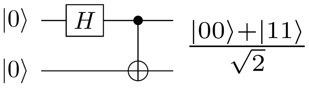
Figure 1: Schematic depiction of a quantum circuit for preparing a maximally entangled $2$-qubit Bell state $\left|\psi_{\mathrm{Bell}_{1}}\right\rangle\overset{\text{def}}{=}(\left|00\right\rangle+\left|11\right\rangle)/\sqrt{2}$ with a $1$-qubit Hadamard gate and a $2$-qubit CNOT gate. The GA representation of $\left|\psi_{\mathrm{Bell}_{1}}\right\rangle$ is given by $\psi_{\mathrm{Bell}_{1}}^{\left(\mathrm{GA}\right)}\overset{\text{def}}{=}\left[\left(1+i\sigma_{2}^{1}i\sigma_{2}^{2}\right)E\right]/\sqrt{2}$ with $E\overset{\text{def}}{=}\left(1-i\sigma_{3}^{1}i\sigma_{3}^{2}\right)/2$ being the $2$-particle correlator.

Interestingly, both abstract spin spaces and abstract index conventions are unnecessary within the MSTA language. Abstract spin spaces are specified by the complex Hilbert space $\mathcal{H}_{2}^{n}$ of $n$-qubit quantum states and contain states that must be acted on by quantum unitary operators. For instance, in the case of Bell states, such operators become the CNOT gates. Furthermore, the MSTA formalism avoids the use of explicit matrix representations and, in addition, right or left multiplication by elements originating from a properly identified geometric algebra play the role of operators. The proper GA is selected based on the type of qubit quantum states being acted upon by the operators. This is an additional indication of the conceptual unification provided by the GA language since “spin (qubit) space” and “unitary operators upon spin space” are united, becoming multivectors in real space. In all honesty, we remark that most GA applications in mathematical physics exhibit this conceptual unification.

CNOT Quantum Gate. Following Ref. NIELSEN , the CNOT quantum gate can be conveniently recast as

$$\hat{U}_{\text{CNOT}}^{12}=\frac{1}{2}\left[\left(\hat{I}^{1}+\hat{\Sigma}_{3}^{1}\right)\otimes\hat{I}^{2}+\left(\hat{I}^{1}-\hat{\Sigma}_{3}^{1}\right)\otimes\hat{\Sigma}_{1}^{2}\right]\text{,}$$ (76)

with the operator $\hat{U}_{\text{CNOT}}^{12}$ denoting the CNOT gate from qubit $1$ to qubit $2$. From Eq. (76), we have

$$\hat{U}_{\text{CNOT}}^{12}\left|\psi\right\rangle=\frac{1}{2}\left(\hat{I}^{1}\otimes\hat{I}^{2}+\hat{\Sigma}_{3}^{1}\otimes\hat{I}^{2}+\hat{I}^{1}\otimes\hat{\Sigma}_{1}^{2}-\hat{\Sigma}_{3}^{1}\otimes\hat{\Sigma}_{1}^{2}\right)\left|\psi\right\rangle\text{.}$$ (77)

Using Eqs. (46) and (77), we get

$$\hat{I}^{1}\otimes\hat{I}^{2}\left|\psi\right\rangle\leftrightarrow\psi\text{, }\hat{\Sigma}_{3}^{1}\otimes\hat{I}^{2}\left|\psi\right\rangle\leftrightarrow-i\sigma_{3}^{1}\psi J\text{, }\hat{I}^{1}\otimes\hat{\Sigma}_{1}^{2}\left|\psi\right\rangle\leftrightarrow-i\sigma_{1}^{2}\psi J\text{, }-\hat{\Sigma}_{3}^{1}\otimes\hat{\Sigma}_{1}^{2}\left|\psi\right\rangle\leftrightarrow i\sigma_{3}^{1}i\sigma_{1}^{2}\psi E\text{.}$$ (78)

Finally, making use of Eqs. (77) and (78), the CNOT gate in the GA language becomes

$$\hat{U}_{\text{CNOT}}^{12}\left|\psi\right\rangle\leftrightarrow\frac{1}{2}\left(\psi-i\sigma_{3}^{1}\psi J-i\sigma_{1}^{2}\psi J+i\sigma_{3}^{1}i\sigma_{1}^{2}\psi E\right)\text{.}$$ (79)

Controlled-Phase Gate. From Ref. NIELSEN , the action of the controlled-phase gate $\hat{U}_{\text{CP}}^{12}$ on $\left|\psi\right\rangle\in\mathcal{H}_{2}^{2}$ is,

$$\hat{U}_{\text{CP}}^{12}\left|\psi\right\rangle=\frac{1}{2}\left[\hat{I}^{1}\otimes\hat{I}^{2}+\hat{\Sigma}_{3}^{1}\otimes\hat{I}^{2}+\hat{I}^{1}\otimes\hat{\Sigma}_{3}^{2}-\hat{\Sigma}_{3}^{1}\otimes\hat{\Sigma}_{3}^{2}\right]\left|\psi\right\rangle\text{.}$$ (80)

From Eqs. (46) and (80), we get

$$\hat{I}^{1}\otimes\hat{I}^{2}\left|\psi\right\rangle\leftrightarrow\psi\text{, }\hat{\Sigma}_{3}^{1}\otimes\hat{I}^{2}\left|\psi\right\rangle\leftrightarrow-i\sigma_{3}^{1}\psi J\text{, }\hat{I}^{1}\otimes\hat{\Sigma}_{3}^{2}\left|\psi\right\rangle\leftrightarrow-i\sigma_{3}^{2}\psi J\text{, }-\hat{\Sigma}_{3}^{1}\otimes\hat{\Sigma}_{3}^{2}\left|\psi\right\rangle\leftrightarrow i\sigma_{3}^{1}i\sigma_{3}^{2}\psi E\text{.}$$ (81)

Finally, using Eqs. (80) and (81), the controlled-phase quantum gate in the GA language reduces to

$$\hat{U}_{\text{CP}}^{12}\left|\psi\right\rangle\leftrightarrow\frac{1}{2}\left(\psi-i\sigma_{3}^{1}\psi J-i\sigma_{3}^{2}\psi J+i\sigma_{3}^{1}i\sigma_{3}^{2}\psi E\right)\text{.}$$ (82)

SWAP Gate. From Ref. NIELSEN , the action of the SWAP gate $\hat{U}_{\text{SWAP}}^{12}$ on $\left|\psi\right\rangle\in\mathcal{H}_{2}^{2}$ is,

$$\hat{U}_{\text{SWAP}}^{12}\left|\psi\right\rangle=\frac{1}{2}\left(\hat{I}^{1}\otimes\hat{I}^{2}+\hat{\Sigma}_{1}^{1}\otimes\hat{\Sigma}_{1}^{2}+\hat{\Sigma}_{2}^{1}\otimes\hat{\Sigma}_{2}^{2}+\hat{\Sigma}_{3}^{1}\otimes\hat{\Sigma}_{3}^{2}\right)\left|\psi\right\rangle\text{.}$$ (83)

Using Eqs. (46) and (83), we have

$$\hat{I}^{1}\otimes\hat{I}^{2}\left|\psi\right\rangle\leftrightarrow\psi\text{, }\hat{\Sigma}_{1}^{1}\otimes\hat{\Sigma}_{1}^{2}\left|\psi\right\rangle\leftrightarrow-i\sigma_{1}^{1}i\sigma_{1}^{2}\psi E\text{, }\hat{\Sigma}_{2}^{1}\otimes\hat{\Sigma}_{2}^{2}\left|\psi\right\rangle\leftrightarrow-i\sigma_{2}^{1}i\sigma_{2}^{2}\psi E\text{, }\hat{\Sigma}_{3}^{1}\otimes\hat{\Sigma}_{3}^{2}\left|\psi\right\rangle\leftrightarrow-i\sigma_{3}^{1}i\sigma_{3}^{2}\psi E\text{.}$$ (84)

Finally, employing Eqs. (83) and (84), the SWAP gate in the GA language becomes,

$$\hat{U}_{\text{SWAP}}^{12}\left|\psi\right\rangle\leftrightarrow\frac{1}{2}\left(\psi-i\sigma_{1}^{1}i\sigma_{1}^{2}\psi E-i\sigma_{2}^{1}i\sigma_{2}^{2}\psi E-i\sigma_{3}^{1}i\sigma_{3}^{2}\psi E\right)\text{.}$$ (85)

In Table II, we display the GA description of the action of some of the most relevant $2$-qubit quantum gates on the GA computational basis $\mathcal{B}_{\left[\mathfrak{cl}^{+}(3)\otimes\mathfrak{cl}^{+}(3)\right]/E}$.

Two-qubit gates	Two-qubit states	GA action of gates on states
CNOT	$\psi$	$\frac{1}{2}\left(\psi-i\sigma_{3}^{1}\psi J-i\sigma_{1}^{2}\psi J+i\sigma_{3}^{1}i\sigma_{1}^{2}\psi E\right)$
Controlled-Phase Gate	$\psi$	$\frac{1}{2}\left(\psi-i\sigma_{3}^{1}\psi J-i\sigma_{3}^{2}\psi J+i\sigma_{3}^{1}i\sigma_{3}^{2}\psi E\right)$
SWAP	$\psi$	$\frac{1}{2}\left(\psi-i\sigma_{1}^{1}i\sigma_{1}^{2}\psi E-i\sigma_{2}^{1}i\sigma_{2}^{2}\psi E-i\sigma_{3}^{1}i\sigma_{3}^{2}\psi E\right)$

Table 2: Geometric algebra description of the action of some of the most relevant $2$-qubit quantum gates on the GA computational basis $\mathcal{B}_{\left[\mathfrak{cl}^{+}(3)\otimes\mathfrak{cl}^{+}(3)\right]/E}$.

Interestingly, two-qubit quantum gates can be geometrically interpreted by means of rotations. For example, the CNOT gate specifies a rotation in one qubit space conditional on the quantum state of a different qubit it is correlated with. In the GA language, this CNOT gate becomes $(\hat{U}_{\text{CNOT}}^{12\left(\text{{GA}}\right)})=e^{-i\frac{\pi}{2}\frac{1}{2}\sigma_{1}^{1}\left(1-\sigma_{3}^{2}\right)}$. In particular, this operator acts as a rotation on the first qubit by an angle $\pi$ about the axis $\sigma_{1}^{1}$ in those $2$-qubit quantum states in which qubit is located along the $-\sigma_{2}^{3}$ axis. For further technical details on analogous geometrically flavored considerations for other $2$-qubit gates, we refer to Ref. somaroo .

In what follows, we briefly discuss the application of the MSTA formalism to density matrices for mixed quantum states.

III.3 Density Operators

It is known that the statistical aspects of quantum systems can be suitably described by density matrices and, instead, cannot be specified by means of a single wave function. For a pure state, the density matrix can be recast as

$$\hat{\rho}_{\text{pure}}=\left|\psi\right\rangle\left\langle\psi\right|=\left(\begin{array}[c]{cc}\alpha\alpha^{\ast}&\alpha\beta^{\ast}\\ \beta\alpha^{\ast}&\beta\beta^{\ast}\end{array}\right)\text{.}$$ (86)

Importantly, the expectation value $\left\langle\hat{O}\right\rangle$ of any observable $\hat{O}$ with respect to a given normalized quantum state $\left|\psi\right\rangle$ can be derived from $\hat{\rho}_{\text{pure}}$ by noting that $\left\langle\hat{O}\right\rangle=\left\langle\psi|\hat{O}|\psi\right\rangle=$tr$(\hat{\rho}_{\text{pure}}\hat{O})$. The formulation of $\hat{\rho}_{\text{pure}}$ in the GA language is given by

$$\hat{\rho}_{\text{pure}}\rightarrow\rho_{\text{pure}}^{\left(\text{{GA}}\right)}=\psi\frac{1}{2}\left(1+\sigma_{3}\right)\psi^{\dagger}=\frac{1}{2}\left(1+s\right)\text{,}$$ (87)

with $s$ denoting the spin vector defined as $s\overset{\text{def}}{=}\psi\sigma_{3}\psi^{\dagger}$ doran96 . From Eq. (87), we observe that $\rho_{\text{pure}}^{\left(\text{{GA}}\right)}$ is simply the sum of a scalar and a vector from a geometric standpoint. In standard quantum mechanics, a density matrix for a mixed quantum state $\hat{\rho}_{\text{mixed}}$ can be expressed in terms of a weighted sum of the density matrices for the pure quantum states as

$$\hat{\rho}_{\text{mixed}}=\sum_{j=1}^{n}\hat{\rho}_{j}=\sum_{j=1}^{n}p_{j}\left|\psi_{j}\right\rangle\left\langle\psi_{j}\right|\text{,}$$ (88)

where $\left\{p_{j}\right\}_{j=1,...,n}$  is a set of (real) probabilities normalized to one (i.e., $p_{1}+$…$+p_{n}=1$, where $0\leq p_{j}\leq 1$ for any $j\in\left\{1,...,n\right\}$). In the GA language, given that the addition operation is well-defined, $\hat{\rho}_{\text{mixed}}$ in Eq. (88) can be expressed in terms of a sum as

$$\hat{\rho}_{\text{mixed}}\rightarrow\rho_{\text{mixed}}^{\left(\text{{GA}}\right)}=\frac{1}{2}\sum_{j=1}^{n}\left(p_{j}+p_{j}s_{j}\right)=\frac{1}{2}\left(1+P\right)\text{.}$$ (89)

The quantity $P$ in Eq. (89) denotes the average spin vector (i.e., the ensemble-average polarization vector) with magnitude $\left\|P\right\|$ satisfying the inequality $\left\|P\right\|\leq 1$. The magnitude $\left\|P\right\|$ is a measure of the degree of alignment among the unit polarization vectors $\left\{s_{j}\right\}$ of the individual elements of the ensemble. For correctness, we emphasize that $\rho_{\text{mixed}}^{\left(\text{{GA}}\right)}$ in Eq. (89) is the GA description of a density operator for an ensemble of identical and non-interacting quantum bits. In general, one could take into consideration expressions of density operators for multi-qubit systems characterized by interacting quantum bits. In the MSTA formalism, the density matrix of $n$-interacting qubits can be recast as

$$\rho_{\text{multi-qubit}}^{\left(\text{{GA}}\right)}=\overline{\left(\psi E_{n}\right)E_{+}\left(\psi E_{n}\right)^{\sim}}\text{.}$$ (90)

In Eq. (90), $E_{n}$ denotes the $n$-particle correlator, while $E_{+}\overset{\text{def}}{=}E_{+}^{1}E_{+}^{2}$…$E_{+}^{n}$ describes the geometric product of $n$-idempotents with $E_{\pm}^{k}\overset{\text{def}}{=}(1\pm\sigma_{3}^{k})/2$ and $k=1$,…, $n$. Finally, while the tilde symbol “$\sim$” is used to describe the space-time reverse, the over-line “$\overline{}$” signifies the ensemble-average. For further technicalities on the GA approach to density matrices for general quantum systems, we suggest Ref. doran1 .

IV Universality of quantum gates with geometric algebra

Employing the results obtained in Section III and, in addition, formulating a GA perspective on the Lie algebras $\mathrm{SO}\left(3\right)$ and $\mathrm{SU}\left(2\right)$ that relies on the rotor group $\mathrm{Spin}^{+}\left(3\text{, }0\right)$ formalism, we discuss in this section a GA-based version of the universality of quantum gates proof as originally proposed by Boykin and collaborators in Refs. B99 ; B00 . We begin with the introduction of the rotor group $\mathrm{Spin}^{+}\left(3\text{, }0\right)$. We then bring in some universal sets of quantum gates. Finally, we discuss our GA-based proof of universality in quantum computing.

IV.1 $\mathrm{SO}(3)$, $\mathrm{SU}(2)$, and $\mathrm{Spin}^{+}(3$, $0)$

Motivated by the fact that the proofs in Refs. B99 ; B00 depend in a significant manner on rotations in three-dimensional space and, in addition, on the local isomorphism between $\mathrm{SO}(3)$ and $\mathrm{SU}(2)$, we briefly show how these Lie groups can be described in the GA language in terms of the rotor group $\mathrm{Spin}^{+}\left(3\text{, }0\right)$.

IV.1.1 Preliminaries on $\mathrm{SO}(3)$ and $\mathrm{SU}(2)$

Three-dimensional Lie groups are very important in physics morton . In this regard, the three-dimensional Lie groups $\mathrm{SO}(3)$ and $\mathrm{SU}(2)$ with Lie algebras $\mathfrak{so(}3\mathfrak{)}$ and $\mathfrak{su(}2\mathfrak{)}$, respectively, are two physically significant groups. The group $\mathrm{SO}(3)$ denotes the group of orthogonal transformations with determinant equal to one (i.e., rotations of three-dimensional space) and is defined by,

$$\mathrm{SO}(3)\overset{\text{def}}{=}\left\{M\in GL(3\text{, }\mathbb{R}):MM^{t}=M^{t}M=I_{3\times 3}\text{, }\det M=1\right\}\text{.}$$ (91)

In Eq. (91), $GL(3$, $\mathbb{R})$ is the general linear group specified by the set of non-singular linear transformations in $\mathbb{R}^{3}$ characterized by $3\times 3$ non singular matrices with real entries. The letter “$t$”, instead, means the transpose of a matrix. The group $\mathrm{SU}(2)$ is the special unitary group all $2\times 2$ unitary complex matrices with determinant equal to one. It is defined as,

$$\mathrm{SU}(2)\overset{\text{def}}{=}\left\{M\in GL(2\text{, }\mathbb{C}):MM^{\dagger}=M^{\dagger}M=I_{2\times 2}\text{, }\det M=1\right\}\text{.}$$ (92)

In Eq. (92), $GL(2$, $\mathbb{C})$ denotes the set of non-singular linear transformations in $\mathbb{C}^{2}$ specified by $2\times 2$ non singular matrices with complex entries, while the symbol “$\dagger$” signifies the Hermitian conjugation operation. Interestingly, while the Lie algebras $\mathfrak{so(}3\mathfrak{)}$ and $\mathfrak{su(}2\mathfrak{)}$ are isomorphic (i.e., $\mathfrak{so(}3\mathfrak{)}\cong\mathfrak{su(}2\mathfrak{)}$), the Lie groups $\mathrm{SO}(3)$ and $\mathrm{SU}(2)$ are only locally isomorphic. This means that they differ at a global level (i.e., far from identity), despite the fact that they are not distinguishable in terms of infinitesimal transformations. This distinguishability at the global level implies that the $\mathrm{SO}(3)$ and $\mathrm{SU}(2)$ do no give rise to a pair of isomorphic groups. In particular, this distinguishability manifests itself in the fact that while a rotation by $2\pi$ is the same as the identity in $\mathrm{SO}(3)$, the $\mathrm{SU}(2)$ group is periodic exclusively under rotations by $4\pi$. This implies that while it is an unacceptable representation of $\mathrm{SO}(3)$, a quantity that acquires a minus sign under the action of a rotation by an angle equal to $2\pi$ represents an acceptable representation of $\mathrm{SU}(2)$. Interestingly, as pointed out in Ref. maggiore , spin-$1/2$ particles (or, alternatively, qubits) need to be rotated by $720^{0}$ (i.e., $4\pi$ radians) to return to the original state. Moreover, while $\mathrm{SU}(2)$ is topologically equivalent to the $3$-sphere $\mathcal{S}^{3}$, $\mathrm{SO}(3)$ is topologically equivalent to the projective space $\mathbb{R}P^{3}$. For completeness, note that $\mathbb{R}P^{3}$ originates from $\mathcal{S}^{3}$ once one identifies pairs of antipodal points. These comparative remarks between the groups $\mathrm{SO}(3)$ and $\mathrm{SU}(2)$ imply that the groups that are actually isomorphic are the quotient group $\mathrm{SU}(2)/\mathbb{Z}_{2}$ and $\mathrm{SO}(3)$ (i.e., $\mathrm{SU}(2)/\mathbb{Z}_{2}\cong\mathrm{SO}(3)$). From a formal mathematical standpoint, there exists an unfaithful representation $\varkappa$ of $\mathrm{SU}(2)$ as a group of rotations in $\mathbb{R}^{3}$,

$$\varkappa:\mathrm{SU}(2)\ni U_{\mathrm{SU}(2)}(\vec{A}\text{, }\theta)\overset{\text{def}}{=}\exp(\frac{\vec{\Sigma}}{2i_{\mathbb{C}}}\cdot\vec{A}\theta)\mapsto R_{\mathrm{SO}(3)}(\vec{A}\text{, }\theta)\overset{\text{def}}{=}\exp(\vec{E}\cdot\vec{A}\theta)\in\mathrm{SO}(3)\text{,}$$ (93)

for any vector $\vec{A}=\left(A_{1}\text{, }A_{2}\text{, }A_{3}\right)$ in $\mathbb{R}^{3}$. For mathematical accuracy, we emphasize that the employment of the dot-notation in Eq. (93) (and, in addition, in the following Eqs. (95), (105), (128)) represents an abuse of notation for the Euclidean inner product. As a matter of fact, while $\vec{A}$ is simply a vector in $\mathbb{R}^{3}$, the quantity $\vec{\Sigma}$  specifies the vector of Pauli operators that act on a two-dimensional complex Hilbert space. Note that the vector $\vec{E}=\left(E_{1}\text{, }E_{2}\text{, }E_{3}\right)$ in Eq. (93) determines a basis of infinitesimal generators of the Lie algebra $\mathfrak{so(}3\mathfrak{)}$ of the group $\mathrm{SO}(3)$,

$$E_{1}\overset{\text{def}}{=}\left(\begin{array}[c]{ccc}0&0&0\\ 0&0&-1\\ 0&1&0\end{array}\right)\text{, }E_{2}\overset{\text{def}}{=}\left(\begin{array}[c]{ccc}0&0&1\\ 0&0&0\\ -1&0&0\end{array}\right)\text{, }E_{3}\overset{\text{def}}{=}\left(\begin{array}[c]{ccc}0&-1&0\\ 1&0&0\\ 0&0&0\end{array}\right)\text{.}$$ (94)

The matrices $\left\{E_{j}\right\}$ with $j\in\left\{1,2,3\right\}$ in Eq. (94) fulfill the commutation relations, $\left[E_{l}\text{, }E_{m}\right]=\varepsilon_{lmk}E_{k}$ with $\varepsilon_{lmk}$ being the usual Levi-Civita symbol. Alternatively, the infinitesimal generators of the Lie algebra $\mathfrak{su(}2\mathfrak{)}$ of the special unitary group $\mathrm{SU}(2)$ are determined by $i_{\mathbb{C}}\vec{\Sigma}=\left(i_{\mathbb{C}}\Sigma_{1}\text{, }i_{\mathbb{C}}\Sigma_{2}\text{, }i_{\mathbb{C}}\Sigma_{3}\right)$. These generators satisfy the commutation relations given by $\left[\Sigma_{l}\text{, }\Sigma_{m}\right]=2i_{\mathbb{C}}\varepsilon_{lmk}\Sigma_{k}$. It is worthwhile mentioning that these latter commutation relations are identical to those for $\mathrm{SO}(3)$ once one employs $\Sigma_{l}/2i_{\mathbb{C}}$ as a new basis for the algebra $\mathfrak{su(}2\mathfrak{)}$. The map $\varkappa$ in Eq. (93) is exactly two-to-one. Therefore,  to a rotation of $\mathbb{R}^{3}$ about an axis specified by a unit vector $\vec{A}$ through an angle of $\theta$ radians, there correspond two $2\times 2$ unitary matrices with determinant equal to one,

$$\exp(\frac{\vec{\Sigma}}{2i_{\mathbb{C}}}\cdot\vec{A}\theta)\text{ and, }\exp[\frac{\vec{\Sigma}}{2i_{\mathbb{C}}}\cdot\vec{A}\left(\theta+2\pi\right)]\text{.}$$ (95)

Put differently, not only $\mathrm{SO}(3)$ possesses the traditional representation in terms of $3\times 3$ matrices, it also enjoys a double-valued representation by means of $2\times 2$ matrices acting on $\mathbb{C}^{2}$. In this respect, spinors can be simply viewed as the complex vectors $(\begin{array}[c]{cc}\psi^{1}&\psi^{2}\end{array})^{t}\in\mathbb{C}^{2}$ on which $\mathrm{SO}(3)$ operates in this double-valued manner. From a mathematical standpoint, $\mathrm{SU}(2)$ offers in a natural manner a spinor representation of the $2$-fold cover of the group $\mathrm{SO}(3)$. Note that $\mathrm{SU}(2)$ is known as the the spin group $\mathrm{Spin}(3)$ when it is viewed as the $2$-fold cover of $\mathrm{SO}(3)$. Representing three-dimensional rotations by means of two-dimensional unitary transformations is extraordinarily effective. In the framework of quantum computing, this is particularly correct when demonstrating particular circuit identities, when characterizing arbitrary $1$-qubit states and, finally, in constructing the Hardy state mermin . To say it all, this representation has a remarkable role in the proof of universality of quantum gates as proposed by Boykin and collaborators in Refs. B99 ; B00 . In particular, the surjective homeomorphism $\varkappa$ in Eq. (93) represents a formidable instrument for studying the product of two or more rotations. This is justified by the fact that Pauli matrices fulfill uncomplicated product rules, $\Sigma_{l}\Sigma_{m}=\delta_{lm}+i_{\mathbb{C}}\varepsilon_{lmk}\Sigma_{k}$. Unfortunately, the infinitesimal generators $\left\{E_{l}\right\}$ with $l\in\left\{1\text{, }2\text{, }3\right\}$ of $\mathfrak{so(}3\mathfrak{)}$ do not satisfy such simple product relations and, for instance, $E_{1}^{2}=\mathrm{diag}\left(0\text{, }-1\text{, }-1\right)$.

Having discussed some links between $\mathrm{SO}(3)$ and $\mathrm{SU}(2)$, we are now ready to introduce the group $\mathrm{Spin}^{+}(3$, $0)$.

IV.1.2 Preliminaries on $\mathrm{Spin}^{+}(3$, $0)$

In the GA language, rotations are described by means of rotors and they represent one of the most significant applications of geometric algebra. Moreover, Lie groups and Lie algebras can be conveniently studied in terms of rotors. In the following, we present some definitions. For further details on the Clifford algebras, we refer to Ref. porto .

Assume that $\mathcal{G}\left(p\text{, }q\right)$ specifies the GA of a space with signature $\left(p\text{, }q\right)$, where $p+q=n$ and $n$ is the dimensionality of the space. Assume, in addition, that $\mathcal{V}$ is the space whose elements are grade-$1$ multivectors. Then, $\mathrm{Pin}\left(p\text{, }q\right)$ is the so-called pin group with respect to the geometric product and is given by,

$$\mathrm{Pin}\left(p\text{, }q\right)\overset{\text{def}}{=}\left\{M\in\mathcal{G}\left(p\text{, }q\right):MaM^{-1}\in\mathcal{V}\text{ }\forall a\in\mathcal{V}\text{, }MM^{\dagger}=\pm 1\right\}\text{,}$$ (96)

with “$\dagger$” specifying the GA reversion operation where, for example, $\left(a_{1}a_{2}\right)^{\dagger}=a_{2}a_{1}$. The elements of the pin group $\mathrm{Pin}\left(p\text{, }q\right)$ can be partitioned into odd-grade and even-grade multivectors. The even-grade elements $\left\{S\right\}$ of the pin group $\mathrm{Pin}\left(p\text{, }q\right)$ generates a subgroup known as the spin group $\mathrm{Spin}\left(p\text{, }q\right)$,

$$\mathrm{Spin}\left(p\text{, }q\right)\overset{\text{def}}{=}\left\{S\in\mathcal{G}_{+}\left(p\text{, }q\right):SaS^{-1}\in\mathcal{V}\text{ }\forall a\in\mathcal{V}\text{, }SS^{\dagger}=\pm 1\right\}\text{,}$$ (97)

with $\mathcal{G}_{+}\left(p\text{, }q\right)$ being the even subalgebra of $\mathcal{G}\left(p\text{, }q\right)$. Then, rotors are nothing but multivectors $\left\{R\right\}$ of the spin group $\mathrm{Spin}\left(p\text{, }q\right)$ that fulfill the additional constraining condition $RR^{\dagger}=+1$. These elements specify the so-called rotor group $\mathrm{Spin}^{+}\left(p\text{, }q\right)$ defined as,

$$\mathrm{Spin}^{+}\left(p\text{, }q\right)\overset{\text{def}}{=}\left\{R\in\mathcal{G}_{+}\left(p\text{, }q\right):RaR^{\dagger}\in\mathcal{V}\text{ }\forall a\in\mathcal{V}\text{, }RR^{\dagger}=+1\right\}\text{.}$$ (98)

For spaces like the Euclidean spaces, $\mathrm{Spin}\left(n\text{, }0\right)=\mathrm{Spin}^{+}\left(n\text{, }0\right)$. For such scenarios, the spin group $\mathrm{Spin}\left(p\text{, }q\right)$ and the rotor group $\mathrm{Spin}^{+}\left(p\text{, }q\right)$ cannot be distinguished.

In the GA language, the double-sided half-angle transformation law that specifies the rotation of a vector $a$ by an angle $\theta$ in the plane spanned by two unit vectors $m$ and $n$ is given by

$$a\rightarrow a^{\prime}\overset{\text{def}}{=}RaR^{\dagger}\text{.}$$ (99)

The rotor $R$ in Eq. (99) is given by,

$$R\overset{\text{def}}{=}nm=n\cdot m+n\wedge m=\exp(-B\frac{\theta}{2})\text{,}$$ (100)

with the bivector $B$ in Eq. (100) being such that,

$$B\overset{\text{def}}{=}\frac{m\wedge n}{\sin(\frac{\theta}{2})}\text{ and, }B^{2}=-1\text{.}$$ (101)

Thanks to the existence of the geometric product in the GA setting, rotors offer a unique ways of characterizing rotations in geometric algebra. From Eq. (100), observe that rotors are mixed-grade multivectors since they are specified by the geometric product of two unit vectors. Since no special significance can be assigned to the separate scalar and bivector terms, the rotor has no meaning on its own. However, observe that the exponential of a bivector always returns to a rotor and, in addition, all rotors near the origin can be recast in terms of the exponential of a bivector. Therefore, since the bivector $B$ has a clear geometric meaning, when the rotor $R$ is expressed in terms of the exponential of the bivector $B$, both $R$ and the vector $RaR^{\dagger}$ gain a clear geometrically neat significance. Once again, this mathematical picture provides an additional illustrative example of one of the hallmarks of GA. Specifically, both geometrically meaningful objects (vectors and planes, for instance) and the elements (operators, for instance) that operate on them (in this example, rotors $\left\{R\right\}$ or bivectors $\left\{B\right\}$) belong to the same geometric Clifford algebra. Observe that there is a two-to-one mapping between rotors and rotations, since $R$ and $-R$ lead to the same rotation. In Fig. $2$, inspired by the graphical depictions by Doran and Lasenby in Ref. dl , we illustrate a rotation in three dimensions from a geometric algebra viewpoint. We stress that one usually thinks of rotations as taking place around an axis in three-dimensions, a concept that does not generalize straightforwardly to any dimension. However, the GA language leads us to regard rotations as taking place in a plane embedded in a higher dimensional space. Therefore, rotations are described by equations that are valid in arbitrary dimensions.

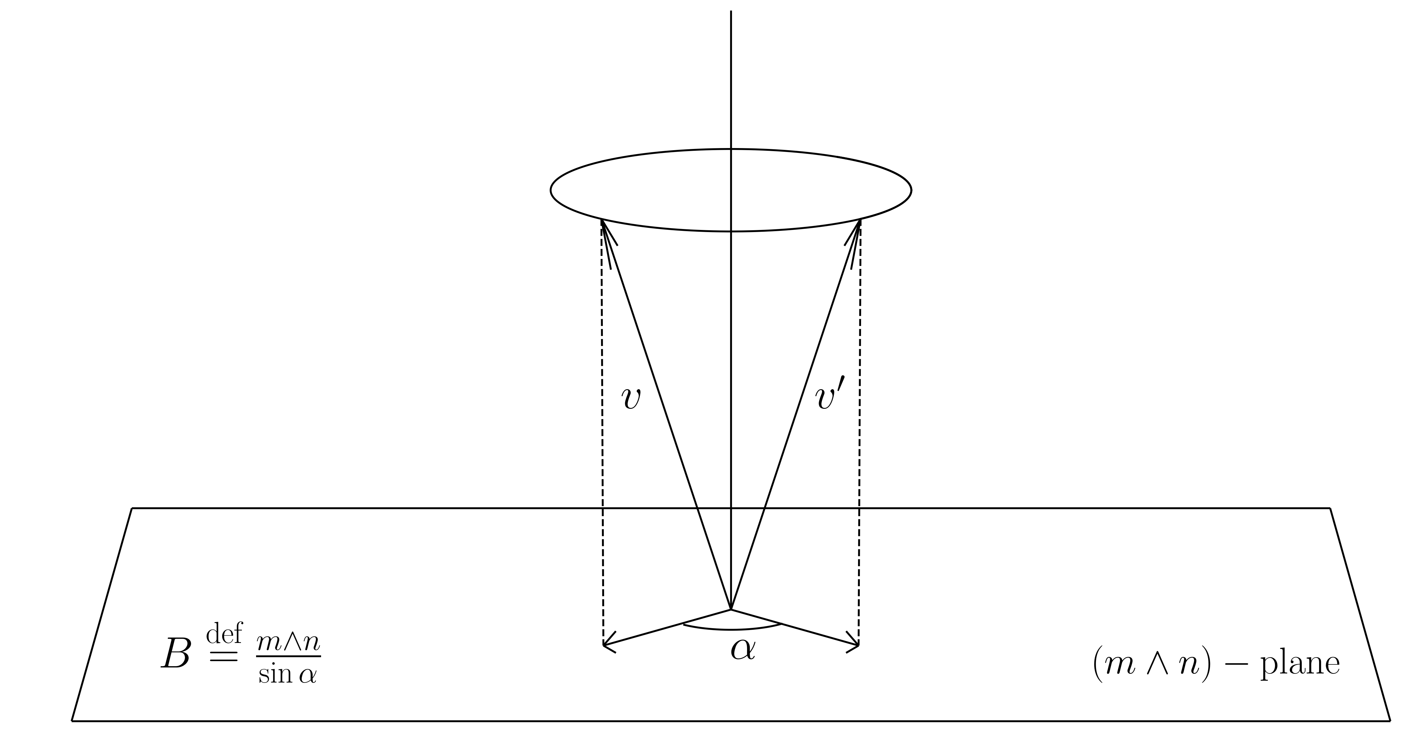
Figure 2: Schematic depiction of a rotation in three dimensions from a geometric algebra viewpoint. The vector $v$ is rotated through an angle $\alpha$ in the $m\wedge n$ plane with $m\cdot n=\cos\left(\alpha\right)$ specified by a unit bivector $B\overset{\text{def}}{=}\left(m\wedge n\right)/\sin(\alpha)$ such that $B^{2}=-1$. After the rotation, $v$ becomes $v^{\prime}=RvR^{\dagger}$ with $R\overset{\text{def}}{=}\exp(-B\alpha/2)$ being the rotor describing the rotation in terms of the $m\wedge n$ plane and the rotation angle $\alpha$.

From a formal mathematical standpoint, the rotor group $\mathrm{Spin}^{+}\left(p\text{, }q\right)$ furnishes a double-cover representation of the rotation group $\mathrm{SO}(n)$. The Lie algebra of the rotor group $\mathrm{Spin}^{+}\left(3\text{, }0\right)$ is determined by means of the bivector algebra relations,

$$\left[B_{l}\text{, }B_{m}\right]=2B_{l}\times B_{m}=-2\varepsilon_{lmk}B_{k}\text{,}$$ (102)

with “$\times$” denoting the commutator product between two multivectors in GA framework. Moreover, the bivectors $\left\{B_{j}\right\}$ with $j\in\left\{1\text{, }2\text{, }3\right\}$ are defined as

$$B_{1}\overset{\text{def}}{=}\sigma_{2}\sigma_{3}=i\sigma_{1}\text{, }B_{2}\overset{\text{def}}{=}\sigma_{3}\sigma_{1}=i\sigma_{2}\text{, }B_{3}\overset{\text{def}}{=}\sigma_{1}\sigma_{2}=i\sigma_{3}\text{.}$$ (103)

Note that the space of bivectors is closed under the commutator product “$\times$”, given the fact that the commutator of a first bivector with a second bivector produces a third bivector. This closed algebra, in turn, specifies the Lie algebra of the corresponding rotor group $\mathrm{Spin}^{+}\left(p\text{, }q\right)$. The act of exponentiation generates the group structure (see Eq. (100)). Moreover, note that the product of bivectors fulfills the following relations,

$$B_{l}B_{m}=-\delta_{lm}-\varepsilon_{lmk}B_{k}\text{.}$$ (104)

The antisymmetric part of $B_{l}B_{m}$ in Eq. (104) is a bivector, whereas the symmetric part of this product denotes a scalar quantity. As a concluding remark, we emphasize that the algebra of the generators of the quaternions is like the algebra of bivectors in GA. For this reason, bivectors correspond to quaternions in the GA language. In Table III, we report in a schematic fashion a comparative description of $\mathrm{SO}(3)$, $\mathrm{SU}(2)$, and $\mathrm{Spin}^{+}\left(p\text{, }q\right)$.

Lie groups	Lie algebras	Product rules	Operator, Vectors
$\mathrm{SO}(3)$	$\left[E_{l}\text{, }E_{m}\right]=\varepsilon_{lmk}E_{k}$	Not useful	Orthogonal transformations, vectors in $\mathbb{R}^{3}$
$\mathrm{SU}(2)$	$\left[\Sigma_{l}\text{, }\Sigma_{m}\right]=2i_{\mathbb{C}}\varepsilon_{lmk}\Sigma_{k}$	$\Sigma_{l}\Sigma_{m}=\delta_{lm}+i_{\mathbb{C}}\varepsilon_{lmk}\Sigma_{k}$	Unitary operators, spinors
$\mathrm{Spin}^{+}\left(3\text{, }0\right)$	$\left[B_{l}\text{, }B_{m}\right]=-2\varepsilon_{lmk}B_{k}$	$B_{l}B_{m}=-\delta_{lm}-\varepsilon_{lmk}B_{k}$	Rotors (or, bivectors), multivectors

Table 3: Schematic description of the relevant relations among $\mathrm{SO}(3)$, $\mathrm{SU}(2)$ and, the rotor group $\mathrm{Spin}^{+}\left(3\text{, }0\right)$.

Summing up, two main aspects of the GA language become visible. First, unlike when struggling with matrices, GA offers a very neat and powerful technique to describe rotations. Second, both geometrically significant quantities (vectors and planes, for example) and the elements (i.e., operators) that act on them (in our discussion, rotors $\left\{R\right\}$ or bivectors $\left\{B\right\}$) are members of the very same GA.

IV.2 Universal Quantum Gates

Spins are discrete quantum variables that can represent both inputs and outputs of suitable input-output devices such as quantum computational gates. Indeed, recollect that a finite rotation can be used to express an arbitrary $2\times 2$ unitary matrix with determinant equal to one,

$$\hat{U}_{\mathrm{SU}\left(2\right)}\left(\hat{n}\text{, }\theta\right)\overset{\text{def}}{=}e^{-i_{\mathbb{C}}\frac{\theta}{2}\hat{n}\cdot\vec{\Sigma}}=\hat{I}\cos(\frac{\theta}{2})-i_{\mathbb{C}}\hat{n}\cdot\vec{\Sigma}\sin(\frac{\theta}{2})\text{.}$$ (105)

For this reason, we are allowed to view a qubit as the state of a spin-$1/2$ particle. In addition, we can regard an arbitrary quantum gate, expressed as a unitary transformation that acts on the state, as a rotation of the spin (modulo an overall phase factor). When any quantum computational task can be accomplished with arbitrary precision thanks to networks that consist solely of replicas of gates from that set, such a set of gates is known to be adequate. In the case in which a network characterized by replicas of only one gate can be used to perform any quantum computation, such a gate expresses an adequate set and, in particular, is known to be universal. The Deutsch three-bit gate is an example of a universal quantum gate D89 . This three-bit gate has a $8\times 8$ unitary matrix representation specified by a matrix $\mathcal{D}_{\text{{universal}}}^{\left(\text{{Deutsch}}\right)}\left(\gamma\right)$. With respect to the network’s computational basis $\mathcal{B}_{\mathcal{H}_{2}^{3}}\overset{\text{def}}{=}\left\{\left|000\right\rangle\text{,}\left|100\right\rangle\text{, }\left|010\right\rangle\text{, }\left|001\right\rangle\text{, }\left|110\right\rangle\text{, }\left|101\right\rangle\text{, }\left|011\right\rangle\text{, }\left|111\right\rangle\right\}$, $\mathcal{D}_{\text{{universal}}}^{\left(\text{{Deutsch}}\right)}\left(\gamma\right)$ becomes

$$\mathcal{D}_{\text{{universal}}}^{\left(\text{{Deutsch}}\right)}\left(\gamma\right)\overset{\text{def}}{=}\left(\begin{array}[c]{cc}I_{6\times 6}&O_{6\times 2}\\ O_{2\times 6}&D_{2\times 2}\left(\gamma\right)\end{array}\right)\text{,}$$ (106)

with $I_{l\times l}$ being the $l\times l$ identity matrix, $O_{m\times k}$ denoting the $m\times k$ null matrix, and the matrix $D_{2\times 2}\left(\gamma\right)$ being given by

$$D_{2\times 2}\left(\gamma\right)\overset{\text{def}}{=}\left(\begin{array}[c]{cc}i_{\mathbb{C}}\cos(\frac{\pi\gamma}{2})&\sin(\frac{\pi\gamma}{2})\\ \sin(\frac{\pi\gamma}{2})&i_{\mathbb{C}}\cos(\frac{\pi\gamma}{2})\end{array}\right)\text{.}$$ (107)

From Eq. (106), we note that the Deutsch gate is determined by the parameter $\gamma$ which can assume any irrational value. The Barenco three-parameter family of universal two-bit gates provides an alternative and equally relevant instance of universal quantum gate B95 . This gate has a $4\times 4$ unitary matrix representation denoted here as $\mathcal{A}_{\text{{universal}}}^{\left(\text{{Barenco}}\right)}\left(\phi\text{, }\alpha\text{, }\theta\right)$. With respect to the network’s computational basis $\mathcal{B}_{\mathcal{H}_{2}^{2}}\overset{\text{def}}{=}\left\{\left|00\right\rangle\text{,}\left|10\right\rangle\text{, }\left|01\right\rangle\text{, }\left|11\right\rangle\right\}$, $\mathcal{A}_{\text{{universal}}}^{\left(\text{{Barenco}}\right)}\left(\phi\text{, }\alpha\text{, }\theta\right)$ is defined as

$$\mathcal{A}_{\text{{universal}}}^{\left(\text{{Barenco}}\right)}\left(\phi\text{, }\alpha\text{, }\theta\right)\overset{\text{def}}{=}\left(\begin{array}[c]{cc}I_{2\times 2}&O_{2\times 2}\\ O_{2\times 2}&A_{2\times 2}\left(\phi\text{, }\alpha\text{, }\theta\right)\end{array}\right)\text{,}$$ (108)

with $I_{l\times l}$ denoting the $l\times l$ identity matrix, $O_{m\times k}$ being the $m\times k$ null matrix, and the matrix $A_{2\times 2}\left(\phi\text{, }\alpha\text{, }\theta\right)$ being defined as

$$A_{2\times 2}\left(\phi\text{, }\alpha\text{, }\theta\right)\overset{\text{def}}{=}\left(\begin{array}[c]{cc}e^{i_{\mathbb{C}}\alpha}\cos(\theta)&-i_{\mathbb{C}}e^{i_{\mathbb{C}}\left(\alpha-\phi\right)}\sin(\theta)\\ -i_{\mathbb{C}}e^{i_{\mathbb{C}}\left(\alpha+\phi\right)}\sin(\theta)&e^{i_{\mathbb{C}}\alpha}\cos(\theta)\end{array}\right)\text{.}$$ (109)

From Eq. (108), we observe that the Barenco gate is characterized by three parameters $\phi$, $\alpha$, and $\theta$. These parameters, in turn, are fixed irrational multiples of $\pi$ and of each other. In general, it happens that almost all two-bit (or, $k$-bits with $k>2$) quantum gates are universal D95 ; L96 . Recall that if an arbitrary unitary quantum operation can be accomplished with arbitrarily small error probability by making use of a quantum circuit that only employs gates from $\mathcal{S}$, then a set of quantum gates $\mathcal{S}$ is known to be universal. In quantum computing, a relevant set of logic gates is provided by

$$\mathcal{S}_{\text{{Clifford}}}\overset{\text{def}}{=}\left\{\hat{H}\text{, }\hat{P}\text{, }\hat{U}_{\text{CNOT}}\right\}\text{.}$$ (110)

The set $\mathcal{S}_{\text{{Clifford}}}$ contains the Hadamard-$\hat{H}$, the phase-$\hat{P}$ and the CNOT-$U_{\text{CNOT}}$ gates and produces the so-called Clifford group. As pointed out in Ref. C98 , this group is the normalizer $\mathcal{N}\left(\mathcal{G}_{n}\right)$ of the Pauli group $\mathcal{G}_{n}$ in $\mathcal{U}\left(n\right)$. While the set of gates in $\mathcal{S}_{\text{{Clifford}}}$ suffices to accomplish fault-tolerant quantum computing, it is insufficiently compelling to carry out universal quantum computation. Fortunately, if the gates in $\mathcal{S}_{\text{{Clifford}}}$ are supplemented with the Toffoli gate S96 , universal quantum computation can be realized by

$$\mathcal{S}_{\text{{universal}}}^{\left(\text{{Shor}}\right)}\overset{\text{def}}{=}\left\{\hat{H}\text{, }\hat{P}\text{, }\hat{U}_{\text{CNOT}}\text{, }\hat{U}_{\text{{Toffoli}}}\right\}\text{.}$$ (111)

As demonstrated by Shor S96 , the addition of the Toffoli gate to the generators of $\mathcal{S}_{\text{{Clifford}}}$ gives rise to the universal set of quantum gates $\mathcal{S}_{\text{{universal}}}^{\left(\text{{Shor}}\right)}$ in Eq. (111). An alternative example of a set of universal logic gates was proposed by Boykin and collaborators in Refs. B99 ; B00 . This different set of gates is defined as,

$$\mathcal{S}_{\text{{universal}}}^{\left(\text{{Boykin et al.}}\right)}\overset{\text{def}}{=}\left\{\hat{H}\text{, }\hat{P}\text{, }\hat{T}\text{, }\hat{U}_{\text{CNOT}}\text{ }\right\}\text{.}$$ (112)

From a physical realization standpoint, the set of gates in Eq. (112) is presumably easier to implement experimentally than the set of gates in Eq. (111) given that the Toffoli gate $\hat{U}_{\text{{Toffoli}}}$ is a three-qubit gate while the $\pi/8$-quantum gate $\hat{T}$ is a one-qubit gate.

We are now ready to revisit, from a GA language standpoint, the proof of universality of the set of quantum gates in Eq. (112) as originally proposed by Boykin and collaborators in Refs. B99 ; B00 .

IV.3 GA description of the universality proof

The universality proof, as originally proposed by Boykin and collaborators in Refs. B99 ; B00 , is quite elegant and relies on two main ingredients. First, it depends on the local isomorphism between the Lie groups $\mathrm{SO}(3)$ and $\mathrm{SU}(2)$. Second, it exploits the geometry of real rotations in three dimensions. In the following, using the rotor group $\mathrm{Spin}^{+}\left(3\text{, }0\right)$ along with the algebra of bivectors (i.e., $\left[B_{l}\text{, }B_{m}\right]=-2\varepsilon_{lmk}B_{k}$), we shall reconsider the proof in the GA language.

One can use two steps to present the universality proof of $\mathcal{S}_{\text{{universal}}}^{\left(\text{{Boykin et al.}}\right)}$ in Eq. (112). In the first step, one needs to demonstrate that the Hadamard gate $\hat{H}$ and the $\pi/8$-phase gate $\hat{T}=$ $\hat{\Sigma}_{3}^{1/4}$ give rise to a dense set in the group $\mathrm{SU}(2)$ where, in the GA language, we have

$$\hat{\Sigma}_{3}^{\alpha}\overset{\text{def}}{=}\left(\begin{array}[c]{cc}1&0\\ 0&e^{i_{\mathbb{C}}\pi\alpha}\end{array}\right)\text{, }\hat{\Sigma}_{3}^{\alpha}\left|\psi\right\rangle\leftrightarrow\psi_{\hat{\Sigma}_{3}^{\alpha}}^{\left(\text{{GA}}\right)}=\sigma_{3}^{\alpha}\psi\sigma_{3}\text{. }$$ (113)

The density of the set $\left\{\hat{H}\text{, }\hat{T}\right\}$ implies that a finite product of $\hat{H}$ and $\hat{T}$ can approximate any element $\hat{U}_{\mathrm{SU}(2)}\in\mathrm{SU}(2)$ to an suitably chosen degree of precision. Put differently, it suffices to possess an approximate implementation of the element $\hat{U}$ with some particular level of accuracy, when a circuit of quantum gates is employed to realize a suitably selected unitary operation $\hat{U}$. Assume we use a unitary transformation $\hat{U}^{\prime}$ to approximate a unitary operation $\hat{U}$. Then, the so-called approximation error $\varepsilon\left(\hat{U}\text{, }\hat{U}^{\prime}\right)$ is a good measure of the quality of the approximation of a unitary transformation $\hat{U}$ in terms of $\hat{U}$ afamm ,

$$\varepsilon\left(\hat{U}\text{, }\hat{U}^{\prime}\right)\overset{\text{def}}{=}\max_{\left|\psi\right\rangle}\left\|\left(\hat{U}-\hat{U}^{\prime}\right)\left|\psi\right\rangle\right\|\text{,}$$ (114)

with $\left\|\psi\right\|=\sqrt{\left\langle\psi|\psi\right\rangle}$ denoting the Euclidean norm of $\left|\psi\right\rangle$ and $\left\langle\cdot|\cdot\right\rangle$ being the usual inner product settled on the complex Hilbert space being considered. In the second step of the universality proof, it is required to stress that all that is needed for universal quantum computing is $\hat{U}_{\text{CNOT}}$ and $\mathrm{SU}(2)$ barenco . The local isomorphism between $\mathrm{SO}(3)$ and $\mathrm{SU}(2)$ must be exploited to demonstrate that $\hat{H}$ and $\hat{T}$ give rise to a dense set in $\mathrm{SU}(2)$. As a matter of fact, using the set of gates $\left\{\hat{H}\text{, }\hat{T}\right\}$, we can generate gates that coincide with rotations in $\mathrm{SO}(3$, $\mathbb{R})$ about two orthogonal axes by angles expressed as irrational multiples of $\pi$. Examine the following two rotations in $\mathrm{SO}(3)$ specified by means of rotors in $\mathrm{Spin}^{+}\left(3\text{, }0\right)$,

$$\mathrm{SO}(3)\ni\hat{U}_{\mathrm{SO}(3)}^{\left(1\right)}\overset{\text{def}}{=}e^{i_{\mathbb{C}}\lambda_{1}\pi\hat{n}_{1}\cdot\vec{\Sigma}}\leftrightarrow e^{in_{1}\lambda_{1}\pi}\in\mathrm{Spin}^{+}\left(3\text{, }0\right)\text{, }\hat{U}_{\mathrm{SO}(3)}^{\left(2\right)}\overset{\text{def}}{=}e^{i_{\mathbb{C}}\lambda_{2}\pi\hat{n}_{2}\cdot\vec{\Sigma}}\leftrightarrow e^{in_{2}\lambda_{2}\pi}\text{, }$$ (115)

with $\lambda_{1}$, $\lambda_{2}$ being irrational numbers in $\mathbb{R}/\mathbb{Q}$. Let us verify that the two rotations in Eq. (115) can be described by means of a convenient combination of elements belonging to $\left\{\hat{H}\text{, }\hat{T}\right\}$ with $\hat{T}=\hat{\Sigma}_{3}^{1/4}$. Given that $\mathrm{SU}(2)/\mathbb{Z}_{2}\cong\mathrm{SO}(3)$, it happens to be that

$$\mathrm{Spin}^{+}\left(3\text{, }0\right)\ni e^{in_{1}\lambda_{1}\pi}\leftrightarrow\hat{U}_{\mathrm{SU}(2)}^{\left(1\right)}\overset{\text{def}}{=}\hat{\Sigma}_{3}^{-1/4}\hat{\Sigma}_{1}^{1/4}\in\mathrm{SU}(2)\text{ and, }e^{in_{2}\lambda_{2}\pi}\leftrightarrow\hat{U}_{\mathrm{SU}(2)}^{\left(2\right)}\overset{\text{def}}{=}\hat{H}^{-1/2}\hat{\Sigma}_{3}^{-1/4}\hat{\Sigma}_{1}^{\frac{1}{4}}\hat{H}^{1/2}\text{,}$$ (116)

with $\hat{\Sigma}_{1}^{1/4}=\hat{H}\hat{\Sigma}_{3}^{1/4}\hat{H}$. Exploiting our findings described in Section III and, in addition, hammering out the technical details in Refs. B99 ; B00 , the rotor representations of $\hat{U}_{\mathrm{SU}(2)}^{\left(1\right)}$ and $\hat{U}_{\mathrm{SU}(2)}^{\left(2\right)}$ become

$$\hat{U}_{\mathrm{SU}(2)}^{\left(1\right)}\leftrightarrow R_{1}=\frac{1}{2}\left(1+\frac{1}{\sqrt{2}}\right)\mathbf{-}\frac{1}{2\sqrt{2}}i\sigma_{1}+\frac{1}{2}\left(1-\frac{1}{\sqrt{2}}\right)i\sigma_{2}+\frac{1}{2\sqrt{2}}i\sigma_{3}\text{,}$$ (117)

and,

$$\hat{U}_{\mathrm{SU}(2)}^{\left(2\right)}\leftrightarrow R_{2}=\frac{1}{2}\left(1+\frac{1}{\sqrt{2}}\right)\mathbf{-}\frac{1}{2}\left(\frac{1}{2}-\frac{1}{\sqrt{2}}\right)i\sigma_{1}+\frac{1}{2}i\sigma_{2}+\frac{1}{2}\left(\frac{1}{2}-\frac{1}{\sqrt{2}}\right)i\sigma_{3}\text{,}$$ (118)

respectively. Note that $R_{1}$ and $R_{2}$ in Eqs. (117) and (118), respectively, denote rotors that belong to $\mathrm{Spin}^{+}\left(3\text{, }0\right)$. Observe that,

$$e^{in_{k}\lambda_{k}\pi}=\cos\left(\lambda_{k}\pi\right)+n_{kx}\sin\left(\lambda_{k}\pi\right)i\sigma_{1}+n_{ky}\sin\left(\lambda_{k}\pi\right)i\sigma_{2}+n_{kz}\sin\left(\lambda_{k}\pi\right)i\sigma_{3}\text{,}$$ (119)

for unit vectors $n_{k}$ with $k=1$, $2$. Therefore, putting $e^{in_{1}\lambda_{1}\pi}=R_{1}$, we obtain

$$\cos\left(\lambda_{1}\pi\right)=\frac{1}{2}(1+\frac{1}{\sqrt{2}})\text{, }n_{1y}\sin\left(\lambda_{1}\pi\right)=\frac{1}{2}(1-\frac{1}{\sqrt{2}})\text{, }n_{1z}\sin\left(\lambda_{1}\pi\right)=\frac{1}{2}\frac{1}{\sqrt{2}}\text{, }n_{1x}=-n_{1z}\text{.}$$ (120)

After some algebraic calculations, the number $\lambda_{1}$ reduces to

$$\lambda_{1}=\frac{1}{\pi}\cos^{-1}\left[\frac{1}{2}(1+\frac{1}{\sqrt{2}})\right]\text{.}$$ (121)

Moreover, the unit vector $n_{1}\overset{\text{def}}{=}n_{1x}\sigma_{1}+n_{1y}\sigma_{2}+n_{1z}\sigma_{3}$ becomes

$$n_{1}=\left(n_{1x}\text{, }n_{1y}\text{, }n_{1z}\right)=\frac{1}{\sqrt{1-\left[\frac{1}{2}(1+\frac{1}{\sqrt{2}})\right]^{2}}}\left(-\frac{1}{2\sqrt{2}}\text{, }\frac{1}{2}(1-\frac{1}{\sqrt{2}})\text{, }\frac{1}{2\sqrt{2}}\right)\text{ .}$$ (122)

Analogously, putting $e^{in_{1}\lambda_{2}\pi}=R_{2}$, we get

$$\cos\left(\lambda_{2}\pi\right)=\frac{1}{2}(1+\frac{1}{\sqrt{2}})\text{, }n_{2y}\sin\left(\lambda_{2}\pi\right)=\frac{1}{2}\text{, }n_{2z}\sin\left(\lambda_{2}\pi\right)=\frac{1}{2}(\frac{1}{2}-\frac{1}{\sqrt{2}})\text{, }n_{2x}=-n_{2z}\text{.}$$ (123)

After some additional algebraic calculations, we have that $\lambda_{2}=\lambda_{1}$. Therefore, from Eq. (121), $\lambda_{2}$ becomes

$$\lambda_{2}=\frac{1}{\pi}\cos^{-1}\left[\frac{1}{2}(1+\frac{1}{\sqrt{2}})\right]\text{.}$$ (124)

The unit vector $n_{2}\overset{\text{def}}{=}n_{2x}\sigma_{1}+n_{2y}\sigma_{2}+n_{2z}\sigma_{3}$, instead, reduces to

$$n_{2}=\left(n_{2x}\text{, }n_{2y}\text{, }n_{2z}\right)=\frac{1}{\sqrt{1-\left[\frac{1}{2}(1+\frac{1}{\sqrt{2}})\right]^{2}}}\left(-\frac{1}{2}(\frac{1}{2}-\frac{1}{\sqrt{2}})\text{, }\frac{1}{2}\text{, }\frac{1}{2}(\frac{1}{2}-\frac{1}{\sqrt{2}})\text{ }\right)\text{.}$$ (125)

As a consistency check, we can verify that Eqs. (122) and (125) imply that $n_{1}\cdot n_{2}=0$. Since $\lambda_{1}=\lambda_{2}=\lambda\in\mathbb{R}/\mathbb{Q}$, any phase factor $e^{i_{\mathbb{C}}\phi}$ can be approximately described by $e^{i_{\mathbb{C}}n\lambda\pi}$ for some $n\in\mathbb{N}$ ,

$$e^{i_{\mathbb{C}}\phi}\approx e^{i_{\mathbb{C}}n\lambda\pi}\text{.}$$ (126)

Eqs. (116) and (126) imply that we possess at least two dense subsets of $\mathrm{SU}(2$, $\mathbb{C})$. They are characterized by $e^{in_{1}\alpha}$ and $e^{i\beta n_{2}}$ where,

$$\alpha\approx\lambda\pi l\text{ ({mod}}2\pi\text{) and, }\beta\approx\lambda\pi l\text{ ({mod}}2\pi\text{),}$$ (127)

with $l\in\mathbb{N}$. We observe that we are allowed to express any element $\hat{U}_{\mathrm{SU}(2)}$ $\in$ $\mathrm{SU}(2$, $\mathbb{C})$ as,

$$\hat{U}_{\mathrm{SU}(2)}=e^{i_{\mathbb{C}}\phi\hat{n}\cdot\vec{\Sigma}}\leftrightarrow e^{in\phi}=e^{in_{1}\alpha}e^{in_{2}\beta}e^{in_{1}\gamma}\text{,}$$ (128)

given that $n_{1}$ and $n_{2}$ in Eqs. (122) and (125), respectively, are orthogonal (unit) vectors. Interestingly, note that the decomposition in Eq. (128) can be regarded as the analogue of the Euler rotations about three orthogonal vectors. Expanding the left-hand-side and the right-hand-side of the second relation in Eq. (128), we get

$$e^{in\phi}=\cos(\phi)+in\sin(\phi)\text{.}$$ (129)

and,

$$e^{in_{1}\alpha}e^{in_{2}\beta}e^{in_{1}\gamma}=\left[\cos(\alpha)+in_{1}\sin(\alpha)\right]\left[\cos(\beta)+in_{2}\sin(\beta)\right]\left[\cos(\gamma)+in_{1}\sin(\gamma)\right]\text{,}$$ (130)

respectively. Recollecting that $n_{1}n_{2}=n_{1}\cdot n_{2}+n_{1}\wedge n_{2}$ and, in addition, that the unit vectors $n_{1}$ and $n_{2}$ are orthogonal, we obtain

$$n_{1}n_{2}=-n_{2}n_{1}\text{.}$$ (131)

Furthermore, keeping in mind the following trigonometric relations

$$\sin\left(\alpha\pm\beta\right)=\sin(\alpha)\cos(\beta)\pm\cos(\alpha)\sin(\beta)\text{ and, }\cos\left(\alpha\pm\beta\right)=\cos(\alpha)\cos(\beta)\mp\sin(\alpha)\sin(\beta)\text{, }$$ (132)

additional manipulation of Eq. (130) along with the employment of Eqs. (131) and (132), yields

$$e^{in\phi}=\cos(\beta)\cos\left(\alpha+\gamma\right)+\cos(\beta)\sin\left(\alpha+\gamma\right)in_{1}+\sin(\beta)\cos\left(\gamma-\alpha\right)in_{2}+\sin(\beta)\sin\left(\gamma-\alpha\right)n_{1}\wedge n_{2}\text{.}$$ (133)

Putting Eq. (129) equal to Eq. (133), we finally get

$$\cos(\phi)=\cos(\beta)\cos\left(\alpha+\gamma\right)$$ (134)

and,

$$n\sin(\phi)=\cos(\beta)\sin\left(\alpha+\gamma\right)n_{1}+\sin(\beta)\cos\left(\gamma-\alpha\right)n_{2}-i\sin(\beta)\sin\left(\gamma-\alpha\right)\left(n_{1}\wedge n_{2}\right)\text{.}$$ (135)

In closing, the parameters $\alpha$, $\beta$ and $\gamma$ can be obtained once Eqs. (134) and (135) are inverted for any element in $\mathrm{SU}(2)$. Then, exploiting the fact that $\hat{U}_{\text{CNOT}}$ and $\mathrm{SU}(2)$ give rise to a universal basis of quantum gates for quantum computation barenco , the GA version of the universality proof as originally proposed in Refs. B99 ; B00 is achieved.

As evident from our work, we reiterate that the GA language offers a very neat and solid technique for encoding rotations which is significantly more powerful than computing with matrices. Moreover, as apparent from several applications of GA in mathematical physics, a conceptually relevant feature of GA appears. Namely, vectors (i.e., grade-$1$ multivectors), planes (i.e., grade-$2$ multivectors), and the operators acting on them (i.e., rotors $R$ and bivectors $B$ in our case) are elements that belong to the very same geometric Clifford algebra.

V Concluding remarks

In this paper, we revisited the usefulness of GA techniques in two particular applications in QIS. In our first application, we offered an instructive MSTA characterization of one- and two-qubit quantum states together with a MSTA description of one- and two-qubit quantum computational gates. In our second application, instead, we used the findings of our first application together with the GA characterization of the Lie algebras $\mathrm{SO}\left(3\right)$ and $\mathrm{SU}\left(2\right)$ in terms of the rotor group $\mathrm{Spin}^{+}\left(3\text{, }0\right)$ formalism to revisit the proof of universality of quantum gates as originally proposed by Boykin and collaborators in Refs. B99 ; B00 . Our main conclusions are two. First of all, in agreement with what was stressed in Ref. laser , we point out that the MSTA approach gives rise to a useful conceptual unification in which multivectors in real space provide a unifying setting for both the complex qubit space and the complex space of unitary operators acting on them. Second of all, the GA perspective on rotations in terms of the rotor group $\mathrm{Spin}^{+}\left(3\text{, }0\right)$ undoubtedly introduces both computational and conceptual benefits compared to ordinary vector and matrix algebra approaches.

Inspired by Ref. mancio11 , we made a serious effort here to write this work with a more pedagogical scope for a wider audience. For this reason, we added visual schematic depictions together with background GA preliminary technical details (including, for instance, Appendix A). Moreover, we were able to highlight most of the very interesting works we have partially inspired throughout these years hild20 ; ed21 ; alves22 ; hild22 ; J22 ; silva23 ; ery23 ; winter23 ; J23 ; J24 ; toffano24 . Finally, as evident from the forthcoming paragraphs, we were able to suggest limitations and, at the same time, proposals for future research directions compatible with the current scientific knowledge at the boundaries between GA and quantum computing (with the concept of entanglement playing a prominent role).

In the following, we present some additional remarks related to our proposed use of GA in QIS.

1. In the ordinary formulation of quantum computing, the essential operation is represented by the tensor product “$\otimes$”. The basic operation in the GA approach to quantum computation, instead, is the geometric (Clifford) product. Unlike tensor products, geometric products have transparent geometric interpretations. Indeed, using the geometric product, one can use a vector $\left(\sigma_{1}\right)$ and a square $\left(\sigma_{2}\sigma_{3}\right)$ to form a cube $\left(\sigma_{1}\sigma_{2}\sigma_{3}\right)$. Alternatively, from two vectors $\left(\sigma_{1}\text{ and }\sigma_{2}\right)$, one can generate an oriented square $\left(\sigma_{1}\sigma_{2}\right)$. Also, among many more possibilities, one can form a square $\left(\sigma_{2}\sigma_{3}\right)$ from a cube $\left(\sigma_{1}\sigma_{2}\sigma_{3}\right)$ and a vector $\left(\sigma_{1}\right)$.

2. (Complex) entangled quantum states in ordinary formulations of quantum computing are replaced by (real) multivectors with a clear geometric interpretation within the GA language. For instance, a general multivector $M$ in $\mathfrak{Cl}(3)$ is a linear combination of blades, geometric products of different basis vectors supplemented by the identity $\mathbf{1}$ (basic oriented scalar),

   $$M\overset{\text{def}}{=}M_{0}\mathbf{1}+\sum_{j=1}^{3}M_{j}\sigma_{j}+\sum_{j<k}M_{jk}\sigma_{j}\sigma_{k}+M_{123}\sigma_{1}\sigma_{2}\sigma_{3}\text{, }$$ (136)

   with $j$, $k=1$, $2$, $3$. In this context, entangled quantum states are viewed as GA multivectors that are nothing but bags of shapes (i.e., points, $1$; lines, $\sigma_{j}$; squares, $\sigma_{j}\sigma_{k}$; cubes, $\sigma_{1}\sigma_{2}\sigma_{3}$).

3. One of the key aspect of GA, that we emphasized in Ref. mancio11 and reiterated in the above point [ii] of this paper, is that  (complex) operators and operands (i.e., states) are elements of the same (real) space in the GA setting. This fact, in turn, is at the root of the increasing number of works advocating for the use of online calculators capable of performing quantum computing operations based on geometric algebra hild22 ; alves22 ; hild22 ; J23 ; J24 . We are proud to see that our original work in Ref. mancio11 has had an impact on these more recent works supporting the use of GA-based online calculators in QIS.

4. Describing and, to a certain extent, understanding the complexity of quantum motion of systems in entangled quantum states remains a truly fascinating problem in quantum physics with several open issues. In QIS, the notion of quantum gate complexity, defined for quantum unitary operators and regarded as a measure of the computational work necessary to accomplish a given task, is a significant complexity measure NIELSEN . It would be intriguing to explore if the conceptual unification between (complex) spaces of  quantum states and of quantum unitary operators acting on such states offered by MSTAs can allow for the possibility of yielding a unifying mathematical setting in which complexities of both quantum states and quantum gates are defined for quantities that belong to the same real multivectorial space. Note that geometric reasoning demands the reality of the multivectorial space. Moreover, we speculate that this conceptual unification may happen to be very beneficial with respect to the captivating link between quantum gate complexity and complexity of the motion on a suitable Riemannian manifold of multi-qubit unitary transformations given by Nielsen and collaborators in Refs. nc ; nc1 .

In view of our quantitative findings revisited here, along with our more speculative considerations, we have reason to believe that the use of geometric Clifford algebras in QIS together with its employment in the characterization of quantum gate complexity appears to be deserving of further theoretical explorations brown19 ; chapman18 ; ruan21 ; cafaroprd22 ; cafaropre22 . Moreover, motivated by our revisitation of GA methods in quantum information science together with our findings appeared in Refs. pra22 ; cqg23 , we think that the application of the GA language (with special emphasis on the concept of rotation) can be naturally extended (for gaining deeper physical insights) to the analysis of the propagation of light with maximal degree of coherence pra22 ; wolf07 ; loudon00 and, in addition, to the characterization of the geometry of quantum evolutions cqg23 ; uzdin12 ; campaioli19 ; dou23 ; huang24 .

We have limited our discussion in this paper to the universality for qubit systems. However, it would be fascinating to explore the usefulness of the GA language in the context of universality problems for higher-dimensional systems, i.e. qudits brylinski02 ; saw17 ; saw17B ; saw22 . Interestingly, for quantum computation by means of qudits cafaroqudit , a universal set of gates is specified by all one-qudit gates together with any additional entangling two-qudit gate brylinski02 (that is, a gate that does not map separable states onto separable states). Finally, it would be of theoretical interest exploiting our work as a preliminary starting point from which extending the use of GA techniques from Grover’s algorithm with qubits alves10 ; chap12 ; caf17 to Grover’s algorithm with qudits niko23 . For the time being, we leave these intriguing scientific explorations as future works.

Appendix A From the algebra of physical space to spacetime algebra

In this Appendix, we present essential elements of the algebra of physical space $\mathfrak{cl}(3)$ together with the spacetime Clifford algebra $\mathfrak{cl}(1,3)$.

A.1 Algebra of physical space $\mathfrak{cl}(3)$

Geometric algebra is Clifford’s generalization of complex numbers and quaternion algebra to vectors in arbitrary dimensions. The result is a formalism in which elements of any grade (including scalars, vectors, and bivectors) can be added or multiplied together is called geometric algebra. For two vectors $a$ and $b$ the geometric product is the sum of an inner product and an outer product given by

$$\vec{a}\text{ }\vec{b}\overset{\text{def}}{=}\vec{a}\cdot\vec{b}+\vec{a}\wedge\vec{b}.$$ (137)

Geometric product is associative and has the crucial feature of being invertible.

In three dimensions where $\vec{a}$ and $\vec{b}$ are three-dimensional vectors the inner product is a scalar (grade-$0$ multivector) and the outer product is a bivector (grade-$2$ multivector). Considering a right-handed frame of orthonormal basis vectors ${\vec{e}_{1},\vec{e}_{2},\vec{e}_{3}}$, we have

$$\vec{e}_{l}\vec{e}_{m}=\vec{e}_{l}\cdot\vec{e}_{m}+\vec{e}_{l}\wedge\vec{e}_{m}=\delta_{lm}+\varepsilon_{lmk}i\vec{e}_{k}$$ (138)

where $i\overset{\text{def}}{=}\vec{e}_{1}\vec{e}_{2}\vec{e}_{3}$ is the pseudoscalar which is a trivector (grade-$3$ multivector) and it is the directed unit volume element. Pauli spin matrices also satisfy a relation similar to Eq. (138). Thus, Pauli spin matrices form a matrix representation of the geometric algebra of physical space. The geometric algebra of three-dimensional physical space (APS) is spanned by one scalar, three vectors, three bivectors, and one trivector which defines a graded linear space of $8=2^{3}$ dimensions called $\mathfrak{cl}(3)$,

$$\mathfrak{cl}(3)\overset{\text{def}}{=}\mathrm{Span}\left\{{1}\text{{; }}{\vec{e}_{1},\vec{e}_{2},\vec{e}_{3}}\text{{; }}{\vec{e}_{1}\vec{e}_{2},\vec{e}_{2}\vec{e}_{3},\vec{e}_{3}\vec{e}_{1}}\text{{; }}{\vec{e}_{1}\vec{e}_{2}\vec{e}_{3}}\right\}\text{.}$$ (139)

We also have that $i^{2}=-1$. Since $\vec{e}_{1},\vec{e}_{2},\vec{e}_{3}$ in the Pauli algebra are given by Pauli spin matrices, we can write $i^{\dagger}=-i$ where “$\dagger$” is the Hermitian conjugate in the Pauli spin matrices. This can give a geometric interpretation of $i$ in quantum mechanics. For a general multivector $\bar{M}$ in $\mathfrak{cl}(3)$ we can write

$$\bar{M}=\alpha+\vec{a}+B+\beta i$$ (140)

where $\alpha$ and $\beta$ are scalars denoted by ${\left\langle\bar{M}\right\rangle}_{0}$, $\vec{a}$ is a vector denoted by ${\left\langle\bar{M}\right\rangle}_{1}$, $B$ is a bivector denoted by ${\left\langle\bar{M}\right\rangle}_{2}$, and $i$ is a trivector denoted by ${\left\langle\bar{M}\right\rangle}_{3}$

$$\bar{M}=\underset{k=0,1,2,3}{\sum}\left\langle\bar{M}\right\rangle_{k}=\left\langle\bar{M}\right\rangle_{0}+\left\langle\bar{M}\right\rangle_{1}+\left\langle\bar{M}\right\rangle_{2}+\left\langle\bar{M}\right\rangle_{3}$$ (141)

A bivector $B$ can be written as $B=i\vec{b}$, where $\vec{b}$ is a vector. Substituting this into Eq. (141) we get

$$\bar{M}=\alpha+\vec{a}+i\vec{b}+i\beta=\text{scalar+ vector+ bivector+ trivector.}$$ (142)

Eq. (142 ) can be rearranged as $($complex scalar + complex vector$)=(\alpha+i\beta)+(\vec{a}+i\vec{b})$ which can be written as

$$\bar{M}=\left\langle\bar{M}\right\rangle_{cs}+\left\langle\bar{M}\right\rangle_{cv}=\left[\left\langle\bar{M}\right\rangle_{rs}+\left\langle\bar{M}\right\rangle_{is}\right]+\left[\left\langle\bar{M}\right\rangle_{rv}+\left\langle\bar{M}\right\rangle_{iv}\right]=M^{0}+\vec{M}$$ (143)

where $\left\langle\bar{M}\right\rangle_{cs}$ is the sum of real and imaginary scalar components,

$$\left\langle\bar{M}\right\rangle_{cs}\overset{\text{def}}{=}M^{0}=\left\langle\bar{M}\right\rangle_{rs}+\left\langle\bar{M}\right\rangle_{is}$$ (144)

while $\left\langle\bar{M}\right\rangle_{cv}$ consists of real and imaginary vector components

$$\left\langle\bar{M}\right\rangle_{cv}\overset{\text{def}}{=}M^{0}=\left\langle\bar{M}\right\rangle_{rv}+\left\langle\bar{M}\right\rangle_{iv}.$$ (145)

This is referred to as a paravector and it is used by Baylis to model spacetime. More details can be found in Refs. baylis04 ; baylis89 ; vaz18 ; vaz19 .

Two involutions can be used, the reversion or Hermitian adjoint “${\dagger}$” and the spatial reverse or Clifford conjugate “${\ddagger}$”. For an arbitrary element multivector $\bar{M}=\alpha+\vec{a}+i\vec{b}+i\beta$, these involutions are defined as,

$$\bar{M}^{{\dagger}}\overset{\text{def}}{=}\alpha+\vec{a}-i\vec{b}-i\beta\text{ and, }\bar{M}^{{\ddagger}}\overset{\text{def}}{=}\alpha-\vec{a}-i\vec{b}+i\beta\text{.}$$ (146)

We use here the following notation $\underline{M}\overset{\text{def}}{=}\bar{M}^{{\ddagger}}$. Useful identities are,

$$\left\langle\underline{M}\right\rangle_{rs}=\frac{1}{4}\left[\underline{M}+\underline{M}^{{\dagger}}+\underline{M}^{{\ddagger}}+\left(\underline{M}^{{\dagger}}\right)^{{\ddagger}}\right]\text{, }\left\langle\underline{M}\right\rangle_{rv}=\frac{1}{4}\left[\underline{M}^{{\ddagger}}+\left(\underline{M}^{{\dagger}}\right)^{{\ddagger}}-\underline{M}-\underline{M}^{{\dagger}}\right]\text{,}$$ (147)

$$\left\langle\underline{M}\right\rangle_{is}=\frac{1}{4}\left[\underline{M}-\underline{M}^{{\dagger}}+\underline{M}^{{\ddagger}}-\left(\underline{M}^{{\dagger}}\right)^{{\ddagger}}\right]\text{, }\left\langle\underline{M}\right\rangle_{iv}=\frac{1}{4}\left[\underline{M}^{{\dagger}}-\underline{M}+\underline{M}^{{\ddagger}}-\left(\underline{M}^{{\dagger}}\right)^{{\ddagger}}\right]\text{.}$$ (148)

Moreover, an important algebra of physical space vector is the vector derivatives $\bar{\partial}$ and $\underline{\partial}\overset{\text{def}}{=}$ $\bar{\partial}^{{\ddagger}}$ defined by,

$$\bar{\partial}=\bar{e}_{\mu}\partial^{\mu}=c^{-1}\partial_{t}-\vec{\nabla}\text{ and, }\underline{\partial}=\text{\@text@baccent{e}}^{\mu}\partial_{\mu}=c^{-1}\partial_{t}+\vec{\nabla}\text{.}$$ (149)

Finally, the d’Alambertian differential wave scalar operator $\square_{\mathfrak{cl}(3)}$ in the APS formalism is,

$$\square_{\mathfrak{cl}\mathrm{l}(3)}\overset{\text{def}}{=}\underline{\partial}\overline{\partial}=\bar{e}_{\mu}^{\nu}\text{\@text@baccent{e}}^{\nu}\partial^{\mu}\partial_{\nu}=\delta_{\nu}^{\mu}\partial^{\mu}\partial_{\nu}=\partial^{\mu}\partial_{\mu}\equiv\partial^{2}=c^{-2}\partial_{t}^{2}-\vec{\nabla}^{2}\text{.}$$ (150)

It describes lightlike traveling waves. For additional technical details on the algebra of physical space $\mathfrak{cl}(3)$, we refer to Ref dl . In the next subsection, we present elements of the spacetime algebra $\mathfrak{cl}(1,3)$.

A.2 Spacetime algebra $\mathfrak{cl}(1,3)$

The spacetime algebra (STA) is constructed based on four orthonormal basis vectors ${\gamma_{0},\gamma_{1},\gamma_{2},\gamma_{3}}$ where $\gamma_{0}$ is timelike and $\gamma_{1},\gamma_{2},\gamma_{3}$ are spacelike vectors and form a right-handed orthonormal basis set such that

$${\gamma_{0}}^{2}=1,\ \ \gamma_{0}.\gamma_{i}=0,\ \ \gamma_{i}\cdot\gamma_{j}=-\delta_{ij};\ \ i,j=1,2,3$$ (151)

which can be summarized as

$$\gamma_{\mu}\cdot\gamma_{\nu}=\eta_{\mu\nu}=\mathrm{diag}(+---);\ \mu,\nu=0,...,3.$$ (152)

There are two types of bivectors given by

$$(\gamma_{i}\wedge\gamma_{j})^{2}=-{\gamma_{i}}^{2}{\gamma_{j}}^{2}=-1\text{, and }(\gamma_{i}\wedge\gamma_{0})^{2}=-{\gamma_{i}}^{2}{\gamma_{0}}^{2}=1\text{.}$$ (153)

Finally, there is the grade-$4$ pseudoscalar is defined by

$$i\overset{\text{def}}{=}\gamma_{0}\gamma_{1}\gamma_{2}\gamma_{3}\text{.}$$ (154)

The spacetime algebra, $\mathfrak{cl}(1,3)$ has $16$ terms which includes one scalar, four vectors $({\gamma_{\mu}})$, six bivectors $({\gamma_{\mu}\wedge\gamma_{\nu}})$, four trivectors $({i\gamma_{\mu}})$, and one pseudoscalar $(i=\gamma_{0}\gamma_{1}\gamma_{2}\gamma_{3})$ which give $2^{4}=16$ dimensional STA. Therefore, a basis for the spacetime algebra is given by

$$\left\{1,\gamma_{\mu},\gamma_{\mu}\wedge\gamma_{\nu},i\gamma_{\mu},i\right\}\text{.}$$ (155)

A general element is written as

$$M\overset{\text{def}}{=}{\sum\limits_{k=0}^{4}}\left\langle M\right\rangle_{k}=\alpha+a+B+ib+i\beta\text{,}$$ (156)

where $\alpha$ and $\beta$ are scalars, $a$ and $b$ are vectors and $B$ is a bivector. The vector generators of spacetime algebra satisfy

$$\gamma_{\mu}\gamma_{\nu}+\gamma_{\nu}\gamma_{\mu}=2\eta_{\mu\nu}.$$ (157)

These relations indicate that the Dirac matrices are a representation of spacetime algebra and Minkowski metric tensor’s nonzero terms are $(\eta_{00}$, $\eta_{11}$, $\eta_{22}$, $\eta_{33})=(1$, $-1$, $-1$, $-1)$. A map between a general spacetime vector $a=a^{\mu}\gamma_{\mu}$ and the even subalgebra of the STA $\mathfrak{cl}^{+}(1,3)$ when $\gamma_{0}$ is the future-pointing timelike unit vector is given by

$$a\gamma_{0}=a_{0}+\vec{a}$$ (158)

where

$$a_{0}=a\cdot\gamma_{0}\text{, }\ \vec{a}=a\wedge\gamma_{0}$$ (159)

and $\vec{a}$ is an ordinary spatial vector in three dimensions which can be interpreted as a spacetime bivector. Since the metric is given by $\eta_{\mu\nu}\overset{\text{def}}{=}\mathrm{diag}(+---)$, the matrix has no zero eigenvalues and a trace equal to $-2$ which is in agreement with $\mathfrak{cl}(1,3)$. If instead, the metric is chosen such that the trace is $+2$, the algebra associated with that would be $\mathfrak{cl}(3,1)$ which is not isomorphic to $\mathfrak{cl}(1,3)$. In geometric algebra, the pseudoscalar which is the highest-grade element determines the metric. For the spacetime Lorentz group, the pseudoscalar satisfies $i^{2}=-1$. Since $n=4$ for this space, $i$ anticommutes with odd-grade and commutes with even-grade multivectors of the algebra

$$iP=\pm Pi$$ (160)

where $(+)$ refers to the case when $P$ is even and $(-)$ is the case when $P$ is odd. An important spacetime vector derivative $\nabla$ is defined by

$$\nabla\overset{\text{def}}{=}\gamma^{\mu}\partial_{\mu}\equiv\gamma^{0}c^{-1}\partial_{t}+\gamma^{i}\partial_{i}.$$ (161)

Post-multiplying by $\gamma^{0}$ gives

$$\nabla\gamma_{0}=c^{-1}\partial_{t}+\gamma^{i}\gamma_{0}\partial_{i}=c^{-1}\partial_{t}-\vec{\nabla}$$ (162)

where $\vec{\nabla}$ is the usual derivative defined in vector algebra. Multiplying the spacetime vector derivative by $\gamma^{0}$ gives

$$\gamma_{0}\nabla=c^{-1}\partial_{t}+\vec{\nabla}\text{.}$$ (163)

Finally, we notice that the spacetime vector derivative satisfies the following relation

$$\square=(\gamma_{0}\nabla)(\nabla\gamma_{0})=c^{-2}\partial_{t}^{2}-\vec{\nabla}^{2}$$ (164)

which is the d’Alembert operator used in the description of lightlike traveling waves. Additional technical details on the spacetime Clifford algebra $\mathfrak{cl}(1,3)$ can be found in dl .

References

• (1) D. Hestenes, Spacetime Algebra, Gordon and Breach, New York (1966).
• (2) C. Doran and A. Lasenby, Geometric Algebra for Physicists, Cambridge University Press (2003).
• (3) A. Lasenby, C. Doran and S. Gull, Gravity, gauge theories and geometric algebra, Phil. Trans. Roy. Soc. Lond. A356, 487 (1998).
• (4) M. R. Francis and A. Kosowsky, Geometric algebra techniques for general relativity, Annals of Physics 311, 459 (2004).
• (5) W. E. Baylis, Electrodynamics: A Modern Geometric Approach, World Scientific (1988).
• (6) C. Cafaro and S. A. Ali, The spacetime algebra approach to massive classical electrodynamics with magnetic monopoles, Adv. Appl. Clifford Alg. 17, 23 (2007).
• (7) C. Cafaro, Finite-range electromagnetic interaction and magnetic charges: Spacetime algebra or algebra of physical space?, Adv. Appl. Clifford Alg. 17, 617 (2007).
• (8) A. Yu. Vlasov, Clifford algebras and universal sets of quantum gates, Phys. Rev. A63, 054302 (2001); A. Yu. Vlasov, Quantum gates and Clifford algebras, arXiv:quant-ph/9907079 (1999).
• (9) T. F. Havel and C. Doran, Geometric algebra in quantum information processing, quant-ph/0004031 (2001).
• (10) S. S. Somaroo, D. G. Cory, and T. F. Havel, Expressing the operations of quantum computing in multiparticle geometric algebra, Phys. Lett. A240, 1 (1998).
• (11) D. Aerts and M. Czachor, Cartoon computation: Quantum-like computing without quantum mechanics, J. Phys. A40, 259 (2007).
• (12) M. Czachor, Elementary gates for cartoon computation, J. Phys. A40, 753 (2007).
• (13) D. Aerts and M. Czachor, Tensor-product versus geometric-product coding, Phys. Rev. A77, 012316 (2008).
• (14) C. Cafaro and S. Mancini, A geometric algebra perspective on quantum computational gates and universality in quantum computing, Adv. Appl. Clifford Algebras 21, 493 (2011).
• (15) D. Hildenbrand, C. Steinmetz, R. Alves, J. Hrdina, and C. Lavor, An online calculator for qubits based on geometric algebra, Lecture Notes in Computer Science 12221, 526 (2020).
• (16) E. Bayro-Corrochano, A survey on quaternion algebra and geometric algebra applications in engineering and computer science 1995–2020, IEEE Access 9, 104326 (2021).
• (17) R. Alves, D. Hildenbrand, J. Hrdina, and C. Lavor, An online calculator for quantum computing operations based on geometric algebra, Adv. Appl. Clifford Algebras 32, 4 (2022).
• (18) D. Hildenbrand, The Power of Geometric Algebra Computing, CRC Press (2022).
• (19) J. Hrdina, A. Navrat, and P. Vasik, Quantum computing based on complex Clifford algebras, Quantum Inf. Process. 21, 310 (2022).
• (20) K. De Silva, A. Mahasinghe, and P. Gunasekara, Some remarks on the Solovay–Kitaev approximations in a C*–algebra setting, Palestine Journal of Mathematics 12, 25 (2023).
• (21) I. Eryganov, J. Hrdina, and A. Navrat, Quantization of two- and three-player cooperative games on QRA, arXiv:math.QA/2310.18067 (2023).
• (22) Z.-P. Xu, R. Schwonnek, and A. Winter, Bounding the joint numerical range of Pauli strings by graph parameters, PRX Quantum 5, 020318 (2024).
• (23) J. Hrdina, D. Hildenbrand, A. Navrat, C. Steinmetz, R. Alves, C. Lavor, P. Vasik, and I. Eryganov, Quantum register algebra: The mathematical language for quantum computing, Quantum Inf. Process. 22, 328 (2023).
• (24) J. Hrdina, D. Hildenbrand, A. Navrat, C. Steinmetz, R. Alves, C. Lavor, P. Vasik, and I. Eryganov, Quantum register algebra: The basic concepts, Lecture Notes in Computer Science 13771, 112 (2024).
• (25) G. Veyrac and Z. Toffano, Geometric algebra Jordan-Wigner transformation for quantum simulation, Entropy 26, 410 (2024).
• (26) A. Lasenby, C. Doran, and S. Gull, 2-spinors, twistors and supersymmetry in the spacetime algebra, in Z. Oziewicz et al., eds., Spinors, Twistors, Clifford Algebras and Quantum Deformations, pp. 233-245, Kluwer Academic, Dordrecht (1993).
• (27) C. Doran, A. Lasenby, and S. Gull, States and operators in the spacetime algebra, Found. Phys. 23, 1239 (1993).
• (28) C. J. L. Doran, A. N. Lasenby, S. F. Gull, S. Somaroo, and A. D. Challinor, Spacetime algebra and electron physics, Adv. Imaging Electron Phys. 95, 271 (1996).
• (29) S. Somaroo, A. Lasenby, and C. Doran, Geometric algebra and the causal approach to multiparticle quantum mechanics, J. Math. Phys. 40, 3327 (1999).
• (30) A. Nielsen and I. L. Chuang, Quantum Computation and Information, Cambridge University Press (2000).
• (31) P. O. Boykin, T. Mor, M. Pulver, V. Roychowdhury, and F. Vatan, On universal and fault-tolerant quantum computing, in Proceedings of the 40th Annual Symposium on Fundamentals of Computer Science, IEEE Press, Los Alamitos-CA (1999).
• (32) P. O. Boykin, T. Mor, M. Pulver, V. Roychowdhury, and F. Vatan, A new universal and fault-tolerant quantum basis, Information Processing Letters 75, 101 (2000).
• (33) D. Hestenes, Observables, operators, and complex numbers in the Dirac theory, J. Math. Phys. 16, 556 (1975).
• (34) P. R. Holland, Causal interpretation of a system of two spin-$\frac{1}{2}$ particles, Phys. Rep. 169, 294 (1988).
• (35) M. Hamermesh, Group Theory and Its Applications to Physical Problems, Dover Publication (1968).
• (36) M. Maggiore, A Modern Introduction to Quantum Field Theory, Oxford University Press (2005).
• (37) N. D. Mermin, Quantum Computer Science, Cambridge University Press (2007).
• (38) I. R. Porteous, Mathematical structure of Clifford algebras, in Lectures on Clifford (Geometric) Algebras and Applications, R. Ablamowicz and G. Sobczyk, Editors; Birkhäuser, pp. 31-52 (2004).
• (39) D. Deutsch, Quantum computational networks, Proc. R. Soc. Lond. A425, 73 (1989).
• (40) A. Barenco, A universal two-bit gate for quantum computation, Proc. R. Soc. Lond. A449, 679 (1995).
• (41) D. Deutsch, A. Barenco, and A. Ekert, Universality in quantum computation, Proc. R. Soc. Lond. A449, 669 (1995).
• (42) S. Lloyd, Almost any quantum logic gate is universal, Phys. Rev. Lett. 75, 346 (1996).
• (43) A. R. Calderbank, E. M. Rains, P. W. Shor, and N. J. A. Sloane, Quantum error correction via codes over $GF\left(4\right)$, IEEE Trans. Inf. Theor. 44, 1369 (1998).
• (44) P. Shor, Fault-tolerant quantum computation, in Proceedings of the $37$th Annual Symposium on Fundamentals of Computer Science, IEEE Computer Society Press, pp. 56-65, Los Alamitos-CA (1996).
• (45) P. Kaye, R. Laflamme and M. Mosca, An Introduction to Quantum Computing, Oxford University Press (2007).
• (46) A. Barenco, C. H. Bennett, R. Cleve, D. P. DiVincenzo, N. Margolus, P. Shor, T. Sleator, J. Smolin, and H. Weinfurter, Elementary gates for quantum computation, Phys. Rev. A52, 3457 (1995).
• (47) A. Lasenby, S. Gull, and C. Doran, STA and the interpretation of quantum mechanics, in Clifford (Geometric) Algebras with Applications in Physics, Mathematics and Engineering, W. E. Baylis, Editor; pp. 147-169, Birkhäuser (1996).
• (48) M. A. Nielsen, M. R. Dowling, M. Gu, and A. C. Doherty, Quantum computation as geometry, Science 311, 1133 (2006).
• (49) M. R. Dowling and M. A. Nielsen, The geometry of quantum computation, Quantum Information & Computation 8, 861 (2008).
• (50) A. R. Brown and L. Susskind, Complexity geometry of a single qubit, Phys. Rev. D100, 046020 (2019).
• (51) S. Chapman, M. P. Heller, H. Marrachio, and F. Pastawski, Toward a definition of complexity for quantum field theory states, Phys. Rev. Lett. 120, 121602 (2018).
• (52) S.-M. Ruan, Circuit Complexity of Mixed States, Ph.D. in Physics, University of Waterloo (2021).
• (53) C. Cafaro and P. M. Alsing, Complexity of pure and mixed qubit geodesic paths on curved manifolds, Phys. Rev. D106, 096004 (2022).
• (54) C. Cafaro, S. Ray, and P. M. Alsing, Complexity and efficiency of minimum entropy production probability paths from quantum dynamical evolutions, Phys. Rev. E105, 034143 (2022).
• (55) C. Cafaro, S. Ray, and P. M. Alsing, Optimal-speed unitary quantum time evolutions and propagation of light with maximal degree of coherence, Phys. Rev. A105, 052425 (2022).
• (56) C. Cafaro and P. M. Alsing, Qubit geodesics on the Bloch sphere from optimal-speed Hamiltonian evolutions, Class. Quantum Grav. 40, 115005 (2023).
• (57) E. Wolf, Introduction to the Theory of Coherence and Polarization of Light, Cambridge University Press (2007).
• (58) R. Loudon, The Quantum Theory of Light, Oxford University Press (2000).
• (59) R. Uzdin, U. Günther, S. Rahav, and N. Moiseyev, Time-dependent Hamiltonians with 100% evolution speed efficiency, J. Phys. A: Math. Theor. 45, 415304 (2012).
• (60) F. Campaioli, W. Sloan, K. Modi, and F. A. Pollok, Algorithm for solving unconstrained unitary quantum brachistochrone problems, Phys. Rev. A100, 062328 (2019).
• (61) F.-Q. Dou, M.-P. Han, and C.-C. Shu, Quantum speed limit under brachistochrone evolution, Phys. Rev. Applied 20, 014031 (2023)
• (62) J.-H. Huang, S.-S. Dong, G.-L. Chen, N.-R. Zhou, F.-Y. Liu, and L.-G. Qin, Shortest evolution path between two mixed states and its realization, Phys. Rev. A109, 042405 (2024).
• (63) J.-L. Brylinski and R. Brylinski, Universal quantum gates. In Mathematics of Quantum Computation, edited by R. K. Brylinski and G. Chen, Chapter 4, pp. 117-134, Chapman and Hall/CRC (2002).
• (64) A. Sawicki and K. Karnas, Universality of single-qudit gates, Ann. Henri Poincare 18, 3515 (2017).
• (65) A. Sawicki and K. Karnas, Criteria for universality of quantum gates, Phys. Rev. A95, 062303 (2017).
• (66) A. Sawicki, L. Mattioli, and Z. Zimboras, Universality verification for a set of quantum gates, Phys. Rev. A105, 052602 (2022).
• (67) C. Cafaro, F. Maiolini, and S. Mancini, Quantum stabilizer codes embedding qubits into qudits, Phys. Rev. A86, 022308 (2012).
• (68) R. Alves and C. Lavor, Clifford algebra applied to Grover’s algorithm, Adv. Appl. Clifford Algebra 20, 477 (2010).
• (69) J. M. Chappell, A. Iqbal, M. A. Lohe, L. von Smekal, and D. Abbott, An improved formalism for quantum computation based on geometric algebra-case study: Grover’s search algorithm, Quantum Information Processing 12, 1719 (2012).
• (70) C. Cafaro, Geometric algebra and information geometry for quantum computational software, Physica A470, 154 (2017).
• (71) A. S. Nikolaeva, E. O. Kiktenko, and A. K. Fedorov, Generalized Toffoli gate decomposition using ququints: Towards realizing Grover’s algorithm with qudits, Entropy 25, 387 (2023).
• (72) W. E. Baylis, Geometry of paravector space with applications to relativistic physics, In: Byrnes, J. (eds.) Computational Noncommutative Algebra and Applications. NATO Science Series II: Mathematics, Physics and Chemistry, Vol. 136. Springer, Dordrecht (2004).
• (73) W. E. Baylis and G. Jones, The Pauli algebra approach to special relativity, J. Phys. A: Math. Gen. 22, 1 (1989).
• (74) J. Vaz and S. Mann, Paravectors and the geometry of 3D Euclidean space, Adv. Appl. Clifford Algebras 28, 99 (2018).
• (75) J. Vaz, On paravectors and their associated algebras, Adv. Appl. Clifford Algebras 29, 32 (2019).