A thorough investigation of the Antiferromagnetic Resonance

Abstract

Antiferromagnetic (AF) compounds possess distinct characteristics that render them promising candidates for advancing the application of spin degree of freedom in computational devices. For instance, AF materials exhibit minimal susceptibility to external magnetic fields while operating at frequencies significantly higher than their ferromagnetic counterparts. However, despite their potential, there remains a dearth of understanding, particularly concerning certain aspects of AF spintronics. In particular, the properties of coherent states in AF materials have received insufficient investigation, with many features extrapolated directly from the ferromagnetic scenario. Addressing this gap, this study offers a comprehensive examination of AF coherent states, shedding new light on both AF and Spin-Flop phases. Employing the Holstein-Primakoff formalism, we conduct an in-depth analysis of resonating-driven coherent phases. Subsequently, we apply this formalism to characterize antiferromagnetic resonance, a pivotal phenomenon in spin-pumping experiments, and extract crucial insights therefrom.

I Introduction and motivation

In recent years, there has been notable advancement in Condensed Matter Physics, particularly within the domain of spintronics research, indicating a forthcoming technological paradigm shift. Leveraging the capabilities of generating and controlling spin currents, there is anticipation for the emergence of a novel class of spintronic-based devices poised to supplant conventional electronic counterparts. Moreover, magnetic materials assume a central role in this pioneering endeavor. Notably, magnetic insulators hold particular intrigue for sustaining spin currents, as they mitigate energy losses and enable higher frequency operations compared to traditional electronic devices pr885.1. Within this framework, Spin-Transfer Torque (STT) and Spin Pumping (SP) processes are frequently employed for the generation, manipulation, and detection of spin currents proximal to interfaces involving magnetic compounds. In the STT process, a spin current is injected into the insulator owing to the accumulation of electronic spin near the interfacejmmm159.L1; prb54.9353. Conversely, SP entails the generation of spin current by employing an oscillating microwave field, which provides angular momentum transferring to the material in contact with the magnetic insulatorprl88.117601.

The SP mechanism entails the utilization of magnetic fields to induce a coherent precession of magnetization. This process involves the alignment of the spin field by a static magnetic field, complemented by an oscillating field that supports coherent dynamics. When the oscillating magnetic field is transversal to the static field, we classify the process as linear, while for oscillating fields parallel to the static field, we have a nonlinear (or parametric) magnon excitation. By adjusting the intensity of the static magnetic field, we reach the resonance when the frequency of long wavelength magnons coincides with the oscillating field frequency. Consequently, there is an amplification in the population of low-energy magnons, which arise as spin currents into materials interfacing with the magnet.

In the course of magnetic resonance experiments, the spin field manifests synchronous dynamics, usually described through Coherent States (CS) formalism. Notably, coherent states, initially employed to conceive a comprehensive quantum model of radiation fields pr131.2766 and FM coherent magnons pla29.47; pla29.616; prb4.201, are characterized by minimal uncertainty and are regarded as exhibiting the more classical-quantum nature rmp62.867. To illustrate, consider a particle confined within a harmonic potential, which is represented by a coherent state. In this context, the system holds a minimum uncertainty, $\Delta x\Delta p=\hbar/2$, and the wave function delineates a dispersionless wave packet that harmonically oscillates around the position of potential minimum. Analogously, the resonant spin field demonstrates semi-classical behavior, with classical fields depicted by the phase angle $\varphi$ around the $z$-axis, and the associated conjugate momentum denoted as $S^{z}$. This approach based on canonically conjugated fields (or operators) is the leading feature of the Self-Consistent Harmonic Approximation (SCHA) jmmm472.1; prb106.054313.

Though originally delineated for Ferromagnetic (FM) materials, both SP and STT processes exhibit analogous efficacy in Antiferromagnetic (AFM) insulatorsprl113.057601. Historically, spintronics predominantly revolved around FM, with comparatively limited attention devoted to AFM. However, AFM spintronics has recently garnered significant interest, demonstrating superiority over FM applications natphy14.220; am2024.1521. AFM insulators, for example, evince insensitivity to external magnetic perturbations and engender negligible stray fields due to the absence of macroscopic magnetization. Moreover, owing to AFM coupling, AFM frequencies extend to the terahertz (THz) range, while FM frequencies are restricted to the gigahertz (GHz) scale. A comprehensive exploration of AFM spintronics is available in various references ptrsa369.3098; natnano.3.231; rmp90.015005; rezende.

Despite the acknowledged significance of AFM materials in spintronic research, the existing framework for describing Antiferromagnetic Resonance (AFMR) is deficient. Presently, much of the understanding regarding AFMR derives from a direct extension of the Ferromagnetic Resonance (FMR) results, yielding outcomes that are only partially accurate jap126.151101. Notably absent in the current depiction of AFMR is an assessment of the coherence level, a factor critical for the applicability of Coherent States (CS). Consequently, a meticulous examination reveals a departure from the prevailing understanding in the literature, indicating that coherence in the Spin-Flop (SF) phase is confined to only one of the two AF modes. Furthermore, the determination of magnetic susceptibilities also necessitates precise knowledge of coherence levels. Therefore, in this work, we employ the Holstein-Primakoff (HP) formalism to present a thorough investigation of the AFMR. Our results contribute to a better understanding of the coherence dynamics of AF models, which is essential to many spintronic experiments.

II Semiclassical approach

In this section we present a brief review of the AFMR by using a semiclassical description. To begin with, we adopt a simple AF model given by the following Hamiltonian

$$H=2J\sum_{\langle i,j\rangle}\bm{S}_{i}^{\prime}\cdot\bm{S}_{j}^{\prime}-D\sum_{i}\left(S_{i}^{z\prime}\right)^{2}-\gamma\hbar\sum_{i}\bm{B}_{i}^{\prime}(t)\cdot\bm{S}_{i}^{\prime},$$ (1)

where $J>0$ denotes the Antiferromagnetic exchange coupling constant, with $\langle i,j\rangle$ standing for nearest-neighbor spin interactions. $D>0$ represents a single-ion anisotropic constant, while $\bm{B}^{\prime}(t)=B_{x}^{\prime}(t)\hat{\imath}^{\prime}+B_{y}^{\prime}(t)\hat{\jmath}^{\prime}+B_{z}^{\prime}\hat{k}\prime$ denotes the magnetic field, and $\gamma=\textsl{g}\mu_{B}/\hbar=2\pi\times 28$GHz/T is the gyromagnetic ratio. Note that, for the sake of consistency, we assume that the spin and magnetic moment align in the same direction, without altering the final results. Furthermore, we apply prime notation to delineate spin components within the laboratory reference frame, whereas the absence of prime notation designates the local reference frame, as described below. Additionally, to simplify notation, directional indices ($x$, $y$, and $z$) will be interchangeably expressed as either subscript or superscript indices, with no substantive difference between the two representations.

For the sake of convenience, we establish the longitudinal direction, denoted as the $z$-axis, along the anisotropy axis, while the transverse components reside within the $xy$-plane. The static magnetic field $B_{z}^{\prime}$, pivotal in determining the phase exhibited by the model, aligns parallel to the anisotropic axis, whereas $B_{x}^{\prime}(t)$ and $B_{y}^{\prime}(t)$ represent the transverse components of the magnetic field. Consequently, we initially adopted an easy-axis model; nonetheless, the inclusion of easy-plane anisotropy necessitates minor adjustments in subsequent developments. Given the absence of substantial magnetization, resulting in the elimination of the demagnetizing field, we express $\bm{B}^{\prime}=\mu_{0}\bm{H}_{\textrm{ext}}^{\prime}$, where $\bm{H}_{\textrm{ext}}^{\prime}$ denotes the external H-field. Generally, in spintronic experiments, we employ monochromatic oscillating fields characterized by a constant frequency $\Omega$. However, such consideration is not necessary from the theoretical perspective. Furthermore, owing to the diminished intensity of the transverse component, wherein $B_{x}^{\prime}\approx B_{y}^{\prime}\ll B_{z}^{\prime}$, we can treat the oscillating field as a perturbation.

Depending on the magnitude of $B_{z}^{\prime}$, two distinct phases emerge as a consequence of the energetic interplay between exchange and Zeeman energies. For a weak longitudinal magnetic field, the dominance of exchange energy results in the spin field assuming the conventional Antiferromagnetic (AF) phase, characterized by Néel ordering, where one sublattice magnetization opposes the direction of the other. Conversely, in the regime of strong magnetic fields, the Zeeman energy surpasses the exchange term, leading to the minimization of total energy in what is called the Spin-Flop (SF) phase. In the SF phase, sublattice magnetizations adopt the configuration depicted in Fig. (1), with $\theta_{A}=-\theta_{B}$.

To ascertain the critical field $B_{\textrm{sf}}$, which delineates the transition between the two phases, we consider the limit of uniform sublattice magnetization defined by $\bm{M}_{l}=\gamma\hbar\bm{S}_{l}/2V_{c}$, where $V_{c}$ is the unit cell volume, and $l=A,B$ denotes the sublattice magnetization. Neglecting the influence of the small oscillating magnetic field, we derive an energy expression given by C E_cl(θ_A,θ_B)=γℏNS2[B_E cos(θ_A+θ_B)-BD2(cos^2θ_A+
+cos^2θ_B)-B_z^′(cosθ_A+cosθ_B)], where $\mathcal{N}$ denotes the number of spins and the exchange and the anisotropic fields are defined by $B_{E}=2zJS/\gamma\hbar$ and $B_{D}=2DS/\gamma\hbar$, respectively. Energy minimization yields the solutions $\theta_{A}=0$ and $\theta_{B}=\pi$ (representing the AF phase), or $\theta_{A}=-\theta_{B}=\arccos[B_{z}^{\prime}/(2B_{E}-B_{D})]$ (characterizing the SF phase). Examination of the energy function reveals that the critical field is defined as $B_{\textrm{sf}}=\sqrt{2B_{E}B_{D}-B_{D}^{2}}$. Therefore, as the field intensity increases from small values, the Néel ordering decreases until the system undergoes a first-order phase transition at $B_{z}^{\prime}=B_{\textrm{sf}}$

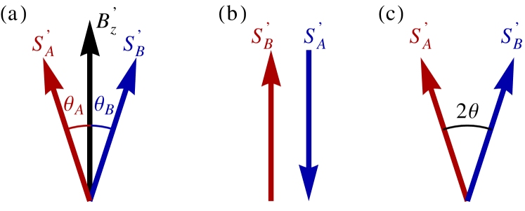
Figure 1: (color online) (a) A general representation of the sublattice magnetizations. The red vector stands for the sublattice A, and the blue represents the sublattice B. (b) For $B_{z}<B_{\textrm{sf}}$, we have the AF phase, which spin field solution is given by $\theta_{A}=0$ and $\theta_{B}=\pi$. (c) For $B_{z}^{\prime}>B_{\textrm{sf}}$, the energy of the SF phase is minimized by the angles $\theta_{A}=-\theta_{B}=\cos^{-1}[B_{z}^{\prime}/(2B_{E}-B_{D})]$.

Restricted to the constraint of a uniform spin field, corresponding to the $q=0$ magnons, the macroscopic magnetization demonstrates behavior analogous to that of a magnetic dipole undergoing precession under the influence of the static field $B_{z}^{\prime}$. Consequently, the magnetization dynamic is given by the Landau-Lifshitz (LL) equation, formulated as $d\bm{M}_{l}/dt=\gamma\bm{M}_{l}\times\bm{B}_{l,\textrm{eff}}$, where $\bm{B}_{l,\textrm{eff}}=-\partial H/\partial\bm{M}_{l}$ denotes the effective magnetic field acting upon sublattice $l$ (the negative sign is absence since we consider that spin and magnetic moment are parallel). By substituting the magnetization ansatz $\bm{M}_{l}(t)=M_{l}^{z}\hat{k}+(m_{l}^{x}\hat{\imath}+m_{l}^{y}\hat{\jmath})e^{-i\omega_{0}t}$ into the LL equation, a system of coupled ordinary differential equations (ODEs) is obtained, yielding the $q=0$ magnon frequencies $\omega_{0}=\gamma B_{z}^{\prime}\pm\gamma(2B_{E}B_{D}+B_{D}^{2})^{1/2}$. In the absence of an external magnetic field, two degenerate modes emerge, precessing in opposing orientations. The frequency of the clockwise mode decreases with increasing $B_{z}^{\prime}$ and vanishes at the critical value $(2B_{E}B_{D}+B_{D}^{2})^{1/2}$, proximal to $B_{\textrm{sf}}$ for small anisotropies.

III Quantum description

To properly describe the quantized spin-waves, we represent the spin operator by employing the HP representation. As usual, to evaluate the magnon spectrum of Eq. (1), it is useful to rotate the spins into a local reference frame, thereby establishing a collinear spin field. Under a generic scenario where each sublattice exhibits a distinct rotation angle, a rotation about the $x$-axis achieves the new spin fields in the local reference frame: rCl S_r,l^x′ &= S_r,l^x
S_r,l^y′ = S_r,l^y cosθ_l - S_r,l^z sinθ_l
S_r,l^z′ = S_r,l^z cosθ_l + S_r,l^y sinθ_l, where $r$ denotes the AF unit cell position and $l=A,B$ signifies the sublattice index. To avoid potential ambiguity, we reserve the indices $i,j$ for site position, which is equally represented by the index pair $r,l$. If we adopt $\mathcal{N}$ as the number of sites, then the number of unit cells is given by $N=\mathcal{N}/2$.

The development follows the usual procedures. Defining the quantization axis along the $z$-axis (in the local reference frame), we use the non-interacting HP representation to write the spin operators as $S_{i}^{z}=S-a_{i}^{\dagger}a_{i}$, $S_{i}^{+}=\sqrt{2S}a_{i}$, and $S_{i}^{-}=\sqrt{2S}a_{i}^{\dagger}$, for the sublattice A. Similarly, for the sublattice B, we achieve $S_{j}^{z}=S-b_{j}^{\dagger}b_{j}$, $S_{j}^{+}=\sqrt{2S}b_{j}$, and $S_{j}^{-}=\sqrt{2S}b_{j}^{\dagger}$. Here, $a$ and $b$ are bosonic operators that satisfy $[a_{i},a_{j}^{\dagger}]=[b_{i},b_{j}^{\dagger}]=\delta_{i,j}$, and $[a_{i},b_{j}^{\dagger}]=[a_{i},b_{j}]=0$. Adopting the low-temperature limit, we can disregard the magnon interactions, and expand the Hamiltonian to second order. Then, after a straightforward procedure, Eq. (1) is expressed as $H(t)=E_{0}+H_{1}(t)+H_{2}$, where the constant term is given by rCl E_0&=γℏN[B_E(S+1)cosΔθ-BD2(S+1)(cos^2θ_A+
+cos^2θ_B)-S(B_A^z+B_B^z)], with $\Delta\theta=\theta_{A}-\theta_{B}$, and $B_{l}^{z}=B_{z}^{\prime}\cos\theta_{l}-B^{y\prime}\sin\theta_{l}$. Performing the Fourier transform $a_{i}=N^{-1/2}\sum_{q}a_{q}e^{iqr}$, and an analogous equation for $b_{i}$, we obtain the time-dependent linear Hamiltonian in momentum space

$$H_{1}(t)=\sum_{q}[h_{q}^{A}(t)a_{q}^{\dagger}+h_{q}^{B}(t)b_{q}^{\dagger}]+\mathrm{h.c.},$$ (2)

where the time-dependent coefficients are rCl h_q^A(t)&=-S2γℏ[i(-B_EsinΔθ+BD2sin2θ_A)Nδ_q,0+
+B_A,q^+(t)], and rCl h_q^B(t)&=-S2γℏ[i(B_EsinΔθ+BD2sin2θ_B)Nδ_q,0+
+B_B,q^+(t)]. In preceding coefficients, we define the magnetic field $B_{l,q}^{+}(t)=B_{q}^{x}(t)+iB_{l,q}^{y}(t)$, where the transformation between the laboratory and local reference frames provides $B_{q}^{x}(t)=B_{q}^{x\prime}(t)$, and $B_{l,q}^{y}(t)=B_{q}^{y\prime}(t)\cos\theta_{l}+B_{q}^{z\prime}\sin\theta_{l}$ for $l=A,B$. As we will see, the linear Hamiltonian is directly responsible for the generation of coherent states, which sustain the magnetization precession. Finally, the quadratic Hamiltonian, which is time-independent, is expressed by

$$H_{2}=\frac{1}{2}\sum_{q}X_{q}^{\dagger}\mathcal{H}_{q}X_{q},$$ (3)

where we define the vector $X_{q}^{\dagger}=(a_{q}^{\dagger}\ b_{q}^{\dagger}\ a_{-q}\ b_{-q})$, and the matrix

$$\mathcal{H}_{q}=\left(\begin{array}[]{cccc}A_{a}&B_{q}&C_{a}&D_{q}\\ B_{q}&A_{b}&D_{q}&C_{b}\\ C_{a}&D_{q}&A_{a}&B_{q}\\ D_{q}&C_{b}&B_{q}&A_{b}\end{array}\right)=I\otimes\mathcal{H}_{q}^{AB}+\sigma_{x}\otimes\mathcal{H}_{q}^{CD},$$ (4)

whose coefficients are given by rCl A_l&=γℏ[-B_EcosΔθ+B_D(cos^2θ_l-sin2θl2)+
+B_z^′cosθ_l],
B_q=γℏ2(1+cosΔθ)B_Eγ_q,
C_l=γℏ2B_Dsin^2θ_l,
D_q=γℏ2 (1-cosΔθ) B_Eγ_q, where $\gamma_{q}=z^{-1}\sum_{\delta r}e^{i\bm{q}\cdot\delta\bm{r}}$ is the structure factor of a lattice defined by $z$ nearest-neighbor spins located at $\delta\bm{r}$ positions.

In accordance with conventional procedures, the diagonalization of the Hamiltonian $H$ is achieved via a Bogoliubov transformation applied to the bosonic operators pr139.a450. To this end, we introduce a new vector operator $\Psi_{q}^{\dagger}=(\alpha_{q}^{\dagger}\ \beta_{q}^{\dagger}\ \alpha_{-q}\ \beta_{-q})$, defined through the linear transformation $X_{q}=T_{q}\Psi_{q}$. In order to preserve the bosonic commutation relation, the matrix transformation must satisfy the condition $T_{q}GT_{q}^{\dagger}=G$, where $G=\sigma_{z}\otimes I$. Consequently, we have:

$$X_{q}^{\dagger}\mathcal{H}_{q}X_{q}=\Psi_{q}^{\dagger}G(T_{q}^{-1}G\mathcal{H}_{q}T_{q})\Psi_{q}=\Psi_{q}^{\dagger}\Omega_{q}\Psi_{q},$$ (5)

where $\Omega_{q}$ is a diagonal matrix given by $\Omega_{q}=\textrm{diag}(\omega_{q}^{\alpha},\omega_{q}^{\beta},\omega_{q}^{\alpha},\omega_{q}^{\beta})$. Technically, the matrix $T_{q}$ diagonalizes $G\mathcal{H}_{q}$; however, determining the transformation for the general case, as defined by Eq. (4), presents an intimidating challenge. Fortunately, under certain symmetrical conditions, exact solutions can be readily obtained for both the AF and SF phases.

Given that the transformation relations between $a_{q}$ and $b_{q}$, the more general transformation $T_{q}$ is expressed as

$$T_{q}=\left(\begin{array}[]{cc}U_{q}&V_{q}\\ \bar{V}_{q}&\bar{U}_{q}\end{array}\right),$$ (6)

where $U_{q}=[u_{mn}]$ and $V_{q}=[v_{mn}]$ are two-dimensional square matrices (the momentum index is implicit in coefficients). Utilizing Eq. (5), it is determined that the submatrices of $T_{q}$ satisfy the following relations: rCl * H_q^AB U_q+H_q^CD¯V_q&=U_qΩ_q,
H_q^AB V_q+H_q^CD¯U_q=-V_qΩ