Unveiling Antiferromagnetic Resonance: A Comprehensive Analysis via the Self-Consistent Harmonic Approximation

Abstract

The Self-Consistent Harmonic Approximation (SCHA) has demonstrated efficacy in discerning phase transitions and, more recently, in elucidating coherent phenomena within ferromagnetic systems. However, a notable gap in understanding arises when extending this framework to antiferromagnetic models. In this investigation, we employ the SCHA formalism to conduct an in-depth exploration of the Antiferromagnetic Resonance (AFMR) within both Antiferromagnetic (AF) and Spin-Flop (SF) phases. Our analysis includes thermodynamic considerations from both semiclassical and quantum perspectives, with comparisons drawn against contemporary experimental and theoretical data. By incorporating a treatment utilizing coherent states, we investigate the dynamics of magnetization precession, a fundamental aspect in comprehending various spintronic experiments. Notably, the SCHA demonstrates excellent agreement with existing literature, showcasing its simplicity and efficiency in describing AFMR characteristics, even close to the transition temperature.

I Introduction and motivation

The Condensed Matter Physics community faces numerous challenges, and the development of spintronic devices occupies a central placescience294.1488; jmmm509.166711. In order to replace electronic-based devices with those that use spin as a degree of freedom, it is essential to have the ability to manipulate spin currents. Magnetic insulators are particularly interesting for sustaining spin currents as they reduce energy losses and provide higher frequency operation than traditional electronic devices pr885.1. In this scenario, Spin-Transfer Torque (STT) and Spin Pumping (SP) are often used for the creation, manipulation, and detection of spin currents in the vicinity of interfaces involving magnetic insulators. In the STT process, a spin current is injected into the insulator due to the spin accumulation near the interfacejmmm159.L1; prb54.9353. In contrast, SP involves the spin current generation by using an oscillating microwave field that provides an angular momentum leaking to the material in contact with the magnetic insulatorprl88.117601. Although these processes were initially described for Ferromagnetic (FM) samples, they work equally well in Antiferromagnetic (AFM) insulatorsprl113.057601. Indeed, for many decades, a considerable fraction of spintronics was primarily based on FM with minor interest in AFM. However, more recently, AFM spintronics has gained attention and proved advantageous over FM applicationsnatphy14.220; am2024.1521. For instance, AFM insulators are insensitive to external magnetic perturbations and provide vanishing stray fields due to the absence of macroscopic magnetization. Additionally, due to the AFM coupling, AFM frequencies reach up to THz while FM frequencies are restricted to the order of GHz. A comprehensive review of AFM spintronics can be found in references ptrsa369.3098; natnano.3.231; rmp90.015005; rezende.

The SP mechanism is widely used to generate spin currents. It involves applying magnetic fields to create a coherent precession of magnetization. A static magnetic field is used to align the spin field, while an oscillating field supports the coherent dynamics. Then, by adjusting the static magnetic field intensity to give long-wavelength magnons with the same frequency as the oscillating field, a resonating condition occurs. This leads to an increasing population of low-energy magnons, which leak as spin currents into materials in contact with the magnet. During those magnetic resonance experiments, the entire spin field exhibits synchronous dynamics, and its behavior is formally described by coherent states, which were initially used to derive a fully quantum model of the radiation fields pr131.2766, as well as coherent magnons pla29.47; pla29.616; prb4.201. Provided that coherent states are the states that show minimum uncertainty, they are considered as the more classical-quantum states rmp62.867. Consider, for instance, a particle in a harmonic potential represented by a Coherent State (CS). In this scenario, $\Delta x\Delta p=\hbar/2$, while the wave function describes a dispersionless wave packet that moves harmonically around the minimum of the potential. The resonating spin field exhibits similar semi-classical behavior, where the classical fields are represented by the phase angle $\varphi$ around the $z$-axis and the conjugate momentum associated, namely $S^{z}$. While in some cases, we adopt $S^{z}$ along the magnetization direction, it is not necessary, and we conveniently chose $S^{z}$ and $S^{y}$ as transverse components, while the magnetization is defined along the $x$-axis, as shown in Fig. 1. Here, we are adopting $\varphi\ll 1$, and thus, the transverse spin components $S^{y}$ and $S^{z}$ are much smaller than the longitudinal component $S^{x}$. In addition, provided that $S^{z}\propto\dot{\varphi}$, both fields $S^{y}$ and $S^{z}$ show an oscillating behavior during the magnetization precession. From the classical perspective, the fields $\varphi_{i}$ and $S^{z}_{j}$, on sites $i$ and $j$, respectively, satisfy the Poisson bracket $\{\varphi_{i},S^{z}_{j}\}=\delta_{ij}$, and the quantization is achieved by promoting the fields to operators that obey the commutation relation $[\varphi_{i},S^{z}_{j}]=\delta_{ij}$. Similar to the particle case, the operators obey the local equality of minimum uncertainty $\Delta\varphi\Delta S^{z}=1/2$, which justifies the semiclassical magnetization behavior of the spin. Therefore it is natural to adopt $\varphi$ and $S^{z}$ as the fundamental operators for describing resonance of magnetic models and the SCHA is the more convenient representation to be used.

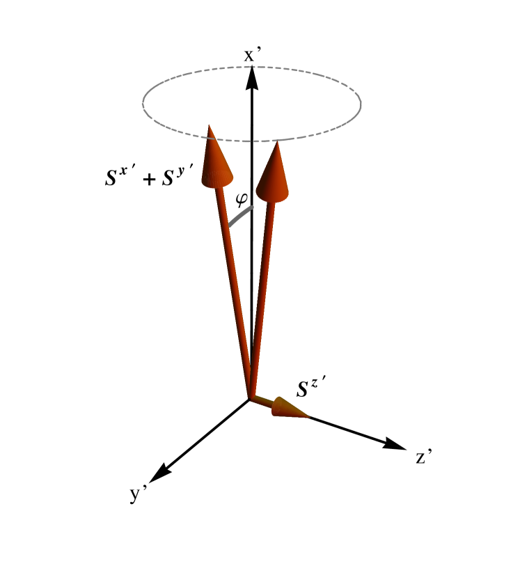
Figure 1: The magnetization and the static magnetic field are defined along the $x$-axis. The angle $\varphi$ is defined as the angle between the spin projection on the xy plane and the $x$-axis.

The fundamental concept underlying the SCHA formalism involves substituting the original spin Hamiltonian with an alternative formulation characterized by solely quadratic terms in the canonically conjugate fields (or operators, within the quantum framework) $\varphi$ and $S^{z}$. Notably, the SCHA diverges from the Holstein–Primakoff (HP) formalism by incorporating spin fluctuations through the self-consistent determination of renormalization parameters, while the latter considers spin-wave interaction by including terms of quartic-order, or higher, in the Hamiltonian. Consequently, the SCHA model exhibits a dual nature, being both straightforward and precise in elucidating the thermodynamics of ordered phases in magnetic materials. Indeed, over the years, the SCHA has been successfully used to determine the critical temperature prb49.9663; pla202.309; prb51.16413; prb54.3019; ssc104.771; prb59.6229, the topological BKT transition pla166.330; prb48.12698; prb49.9663; prb50.9592; ssc100.791; prb53.235; prb54.3019; prb54.6081; ssc112.705; epjb2.169; pssb.242.2138; prb78.212408; jmmm452.315, and the large-D quantum phase transition pasma373.387; jpcm20.015208; pasma388.21; pasma388.3779; jmmm357.45 in a wide variety of magnetic models. Furthermore, the SCHA provides a highly convenient formalism for describing coherent states in ferromagnetic models and spintronic experiments, as exemplified in the references jmmm472.1 and prb106.054313.

In the present study, we extend the preceding SCHA outcomes, originally derived for ferromagnetic models, to systematically examine Antiferromagnetic Resonance (AFMR). While the fundamental conceptualization of AFMR parallels that of the ferromagnetic model, nuanced considerations demand scrutiny. For instance, the presence of diverse phases, contingent upon the static magnetic field intensity, is well-established, presenting a distinctive characteristic absent in Ferromagnetic Resonance (FMR). Consequently, through the application of the SCHA formalism, we obtain a comprehensive elucidation of the coherent behavior of Antiferromagnetic models. This detailed analysis represents a crucial advancement in characterizing the intricacies of antiferromagnetic spintronics.

II Brief Review of AF models

To begin with, we first briefly review the basic concepts of AFMR. We adopt a simple AF model given by the following Hamiltonian

$$H=2J\sum_{\langle i,j\rangle}\bm{S}_{i}^{\prime}\cdot\bm{S}_{j}^{\prime}-D\sum_{i}\left(S_{i}^{x\prime}\right)^{2}-\textsl{g}\mu_{B}\sum_{i}\bm{B}_{i}^{\prime}(t)\cdot\bm{S}_{i}^{\prime},$$ (1)

where $J>0$ is the AF exchange coupling constant, $\langle i,j\rangle$ represents nearest-neighbor spin interactions, $D>0$ is a single-ion anisotropic constant, and $\bm{B}^{\prime}(t)=B_{x}^{\prime}\hat{\imath}^{\prime}+B_{y}^{\prime}(t)\hat{\jmath}^{\prime}+B_{z}^{\prime}(t)\hat{k}^{\prime}$ is the magnetic field. We are adopting prime notation to represent spin components in the laboratory reference frame, while the notation without prime will be used to designate the local reference frame, as described below. Additionally, to clarify the notation, the direction index will be write as either a subscript or superscript index, with no physical difference between them.

For the sake of clarity and without affecting the outcomes, we have opted to align the spin parallel to the magnetic moment in order to simplify the analysis. Additionally, for convenience, we define the $x$-axis, the longitudinal direction, along the anisotropy axis while the transverse components lay on the $yz$-plane. The static magnetic field $B_{x}^{\prime}$, which determines the kind of phase presented by the model, is applied parallel to the anisotropic axis while $B_{y}^{\prime}(t)$ and $B_{z}^{\prime}(t)$ are the transverse magnetic field components. Therefore, we are leading with an easy-axis model; however, including easy-plane anisotropy is straightforward and requires minor changes in the next developments. Since there is no meaningful magnetization, and so the demagnetizing field vanishes, we write $\bm{B}^{\prime}=\mu_{0}\bm{H}_{\textrm{ext}}^{\prime}$, where $\bm{H}_{\textrm{ext}}^{\prime}$ is the external H-field, which is regulated in laboratory. In addition, due to the small intensity of the transverse component, $B_{y}^{\prime}\approx B_{z}^{\prime}\ll B_{x}^{\prime}$, we can consider the oscillating field as a perturbation.

Depending on the intensity of $B_{x}^{\prime}$, we can get two different phases resulting from the energetic dispute between the Exchange and Zeeman energies. For small $B_{x}^{\prime}$ field, the Exchange energy prevails and the spin field assumes the usual AF phase (Néel ordering) where one sublattice magnetization points in the opposite direction of the other one. In the strong field limit, the Zeeman energy exceeds the Exchange term and the total energy is minimized by the so-called Spin-Flop (SF) phase, where the sublattice magnetization assume the configuration shown in Fig. 2 with $\theta_{A}=-\theta_{B}$. To determine the critical field $B_{\textrm{sf}}$, where $sf$ stands for spin-flip, that separates the two phases, we consider the uniform sublattice magnetization limit defined by $\bm{M}_{l}=\gamma\hbar\bm{S}_{l}/2V_{c}$, where $\gamma=g\mu_{B}/\hbar=2\pi\times 28$GHz/T is the gyromagnetic ratio, $V_{c}$ is the unit cell volume, and $l=A,B$ indicates the magnetization sublattice. Disregarding the small oscillating magnetic field, we obtain an energy expression depending on the local angles given by C E(θ_A,θ_B)=γℏNS2[B_E cos(θ_A+θ_B)-BD2(cos^2θ_A+
+cos^2θ_B)-B_x^′(cosθ_A+cosθ_B)], where $\mathcal{N}$ is the number of spins and the exchange and anisotropic fields are defined by $B_{E}=2zJS/\gamma\hbar$ and $B_{D}=2DS/\gamma\hbar$, respectively. The energy minimization provides the solutions $\theta_{A}=0$ and $\theta_{B}=\pi$ (AF phase) or $\theta_{A}=-\theta_{B}=\arccos[B_{x}^{\prime}/(2B_{E}-B_{D})]$ (SF phase), and the analysis of the energy shows that the critical field is given by $B_{\textrm{sf}}=\sqrt{2B_{E}B_{D}-B_{D}^{2}}$. Therefore, as the field intensity increases from small values, the Néel ordering decreases until the system undergoes a first-order phase transition at $B_{x}^{\prime}=B_{\textrm{sf}}$.

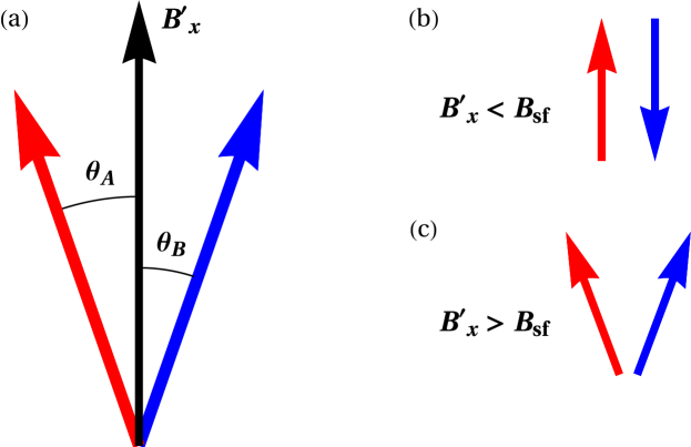
Figure 2: (color online) (a) A general representation of the sublattice magnetizations. The red vector stands for the sublattice A, and the blue represents the sublattice B. (b) For $B_{x}<B_{\textrm{sf}}$, we have the AF phase, which spin field solution is given by $\theta_{A}=0$ and $\theta_{B}=\pi$. (c) For $B_{x}^{\prime}>B_{\textrm{sf}}$, the energy of the SF phase is minimized by the angles $\theta_{A}=\theta_{B}=\cos^{-1}[B_{x}^{\prime}/(2B_{E}-B_{D})]$.

Under the constraint of a uniform spin field, corresponding to the $q=0$ magnons, the macroscopic magnetization exhibits behavior akin to a magnetic dipole undergoing precession within the influence of the static field $B_{x}^{\prime}$. Consequently, the dynamic evolution is governed by the Landau-Lifshitz (LL) equation, expressed as $d\bm{M}_{l}/dt=\gamma\bm{M}_{l}\times\bm{B}_{l,\textrm{eff}}$, where $\bm{B}_{l,\textrm{eff}}=-\partial H/\partial\bm{M}_{l}$ represents the effective magnetic field acting on the sublattice $l$. Substituting the magnetization ansatz $\bm{M}_{l}(t)=M_{l}^{x}\hat{\imath}+(m_{l}^{y}\hat{\jmath}+m_{l}^{z}\hat{k})e^{-i\omega_{0}t}$ into the LL equation, we obtain a coupled set of ODEs that provides the $q=0$ magnon frequencies $\omega_{0}=\gamma B_{x}^{\prime}\pm\gamma(2B_{E}B_{D}+B_{D}^{2})^{1/2}$. In the absence of an external magnetic field ($B_{x}^{\prime}=0$), two degenerate modes emerge, precessing in opposite orientations. The frequency of the clockwise mode decreases with increasing $B_{x}^{\prime}$ and vanishes at the critical value $(2B_{E}B_{D}+B_{D}^{2})^{1/2}$, which is close to $B_{\textrm{sf}}$ for small anisotropies.

As usual, to determine the magnon spectrum of Eq. (1), it is advantageous to transform the spins into a local reference frame, thereby establishing a collinear spin field. Considering a generic scenario, wherein each sublattice manifests a distinct rotating angle, a rotation around the $z$-axis is implemented to attain the new spin fields, in the local reference frame, rCl S_r,l^x′ &= S_r,l^x cosθ_l - S_r,l^y sinθ_l
S_r,l^y′ = S_r,l^x sinθ_l + S_r,l^y cosθ_l
S_r,l^z′ = S_r,l^z, where $r$ represents the AF unit cell position and $l=A,B$ is the sublattice index. To avoid confusion, we reserve the $i,j$ indexes for site position, which is equivalently represented by the index pair $r,l$.

III SCHA

III.1 Semiclassical approach

In the preceding section, we derived the magnon energy for $q=0$ utilizing the LL phenomenological approach. To determine the complete energy spectrum, various established methodologies can be employed, including the HP spin representation. While the HP formalism yields good results in scenarios involving non-interacting spin-waves, its extension to the high magnon density necessitates the inclusion of quartic-order or higher terms. Assessing the impacts of these high-order interaction terms is a complex undertaking, and whenever possible, it is advisable to avoid it. Conversely, the SCHA presents a quadratic model that yields satisfactory outcomes even close to the phase transition temperature. This agreement is achieved by the temperature-dependent renormalization parameters, which consider magnon interactions beyond the scope of second-order expansion. In this context, we employ the SCHA to explore the model described by Equation (1). Initially, we adopt the semiclassical limit to express the spin components in terms of the fields $\varphi$ and $S^{z}$. Subsequently, quantization is obtained by promoting the field to appropriate operators.

From the semiclassical perspective, the spin field is written in terms of the canonically conjugate fields $\varphi$ and $S^{z}$ as $\bm{S}=\sqrt{S^{2}-(S^{z})^{2}}(\cos\varphi\hat{\imath}+\sin\varphi\hat{\jmath})+S^{z}\hat{k}$, which provides the Hamiltonian (in the local reference frame) C H=2J∑_⟨i,j⟩[f_if_j(cosΔθcosΔφ_ij+sinΔθsinΔφ_ij)+
+S_i^z S_j^z]-∑_i{fi22D(cos2θ_icos2φ_i-sin2θ_i sin2φ_i+
+1)+gμ_B[f_i (B_i^xcosφ_i+B_i^ysinφ_i)+ B_i^zS_i^z]}, where $f_{i}=\sqrt{S^{2}-(S_{i}^{z})^{2}}$, $\Delta\theta=\theta_{A}-\theta_{B}$, $\Delta\varphi_{ij}=\varphi_{j}-\varphi_{i}$, $B_{i}^{x}=B^{x\prime}\cos\theta_{l}+B_{i}^{y\prime}\sin\theta_{i}$, $B_{i}^{y}=B_{i}^{y\prime}\cos\theta_{i}-B^{x\prime}\sin\theta_{i}$, and $B_{i}^{z}=B_{i}^{z\prime}$. We consider that the static uniform magnetic field is uniform with $B^{x}\gg B_{i}^{y},B_{i}^{z}$, and $\theta_{i}$ can be $\theta_{A}$ or $\theta_{B}$ depending on the sublattice site. For determining the quadratic model, we expand the Hamiltonian up to second order in $\varphi$ and $S^{z}$. In a naive approximation, the expansion can be done without any correction. However, better results are obtained with the inclusion of renormalization parameters that consider the contributions of higher-order terms. In the SCHA, we include a renormalization factor $\rho$ for each term that presents a trigonometric function expansion. Therefore, in the series expansion, we replace $\varphi$ by $\sqrt{\rho}\varphi$, in which the renormalization parameter is then found by solving a self-consistent equation. After a straightforward procedure, we write the Hamiltonian as $H=E_{0}+H_{1}+H_{2}$, where rCl E_0&=γℏNS[B_EcosΔθ-BD2(cos^2θ_A+cos^2θ_B)-
-(B_A^x+B_B^x)] is the ground state energy, l H_1=γℏ∑_q{Sρ[N(B_EsinΔθ+BD2sin2θ_A)δ_q,0-
-B_A,q^y]φ_A,q+Sρ[N(-B_EsinΔθ+BD2sin2θ_B)δ_q,0-
-B_B,q^y]φ_B,q-B_z,q(S_A,q^z+S_B,q^z)} is a linear term for uniform fields that will be considered as a potential, responsible for the coherent state, and

$$H_{2}=\frac{1}{2}\sum_{q}\sum_{ll^{\prime}}[S^{2}\rho\bar{\varphi}_{l}h_{ll^{\prime}}^{\varphi}\varphi_{l^{\prime}}+\bar{S}_{l}^{z}h_{ll^{\prime}}^{z}S_{l^{\prime}}^{z}]$$ (2)

is the quadratic Hamiltonian, which represents the non-interacting spin-waves endowed the temperature dependent renormalization parameter $\rho$. Here, to make the notation clear, we hidden the momentum index in the $\varphi$ and $S^{z}$ field as well as in the $h$ matrix coefficients. The momentum space is defined in relation to the reciprocal lattice of AF unit cells, and the summation over momenta is evaluated over the first Brillouin zone. $N$ specifies the number of unit cells, while $\mathcal{N}=2N$ is the number of sites. In above equation, the matrix coefficients are given by rCl * h_AA^φ&=γℏS(-B_EcosΔθ+B_Dcos2θ_A+B_A