A logical qubit-design with geometrically tunable error-resistibility

Abstract

Breaking the error-threshold would mark a milestone in establishing quantum advantage for a wide range of relevant problems. One possible route is to encode information redundantly in a logical qubit by combining several noisy qubits, providing an increased robustness against external perturbations. We propose a setup for a logical qubit built from superconducting qubits (SCQs) coupled to a microwave cavity-mode. Our design is based on a recently discovered geometric stabilizing mechanism in the Bose-Hubbard wheel (BHW), which manifests as energetically well-separated clusters of many-body eigenstates. We investigate the impact of experimentally relevant perturbations between SCQs and the cavity on the spectral properties of the BHW. We show that even in the presence of typical fabrication uncertainties, the occurrence and separation of clustered many-body eigenstates is extremely robust. Introducing an additional, frequency-detuned SCQ coupled to the cavity yields duplicates of these clusters, that can be split up by an on-site potential. We show that this allows to (i) redundantly encode two logical qubit states that can be switched and read out efficiently and (ii) can be separated from the remaining many-body spectrum via geometric stabilization. We demonstrate at the example of an $X$-gate that the proposed logical qubit reaches single qubit-gate fidelities $>0.999$ in experimentally feasible temperature regimes $\sim 10-20\,\mathrm{mK}$.

I Introduction

Quantum algorithms obtain polynomial and super-polynomial speed-ups compared to classical algorithms [1, 2] on a selected set of problems [3]. During the past decades, this promise has given rise to the development of schemes that mitigate effects of noise and errors, which typically set a time limit to store and process information in a physical system [4]. Importantly, it has been shown that qubit error rates below a certain threshold allow for arbitrarily accurate quantum computation [5, 6, 7]. Hence, lowering error rates below this threshold marks the central endeavor towards the practical application of quantum algorithms.

To account for the ubiquitous presence of error sources, corrupting both the information represented by the qubit as well as its readout, error correction schemes, such as error mitigation [8, 9, 10] or error correction codes [11, 12, 13, 14] have been introduced. These strategies share the underlying idea that information is represented redundantly and/or non-locally, and can be recovered by repeated measurements or operations on an ensemble of qubits [15, 16]. One prominent approach is quantum error mitigation, aiming for a reduction of the effect of noisy qubit operations by analyzing the structure of the noise. Using repeated circuit runs and measurements, unbiased estimators [10] can be constructed, which has been shown recently to yield promising results [17], yet the corresponding circuit could also be simulated classically [18]. Furthermore, error mitigation schemes share the limitation that the amount of circuit runs grows exponentially with the error probability [10, 19] such that increasing the noise resilience is essential.

A conceptionally different approach are error-correction codes, which distribute the quantum information non-locally such that measurements allow for an active correction [20, 21, 22, 23]. However, the main obstacle is the introduced overhead, shifting the problem of implementing fault-tolerant quantum computation to that of realizing quantum processors with a significantly larger number of physical qubits than operational, logical qubits. Nevertheless, very recently, remarkable progress has been achieved in addressing that problem, for instance using reconfigurable atom arrays [24].

While reconfigurable atom arrays are developing quickly, the most prominent platform are superconducting qubits (SCQs) which have become the backbone of recent advances in fabricating quantum processors [25, 26] and brought forward new possibilities to compose logical qubits out of several SCQ elements [27, 28, 29]. One of the driving forces behind the enormous success of SCQ -based architectures is the possibility to engineer properties such as the anharmonicities via a precise operational control of their constituting circuit elements [30]. However, given current error-rates, the applicability of  SCQ -based quantum processors to practical problems that are out of reach for classical simulations has not been proven so far. Here, the main obstacles are the rather high error rates combined with the limited connectivity that require a vast amount of $100-1000$ SCQs per logical qubit to reach the error threshold for error-correction codes, or a practically unfeasible amount of measurements to apply error mitigation.

In this work we suggest an approach to construct a logical qubit which could address these problems. Using established SCQ -based technologies, our construction achieves a high resilience against external perturbations and is composed of only a small number of qubits $\sim\mathcal{O}(10)$ coupled to a cavity mode. Our proposal is based on the clustering and separation of many-body eigenstates of the Bose-Hubbard wheel (BHW), illustrated in Fig. 1a, in the limit of infinitely strong repulsive interactions [31, 32, 33, 34]. The separation of the energetically lowest cluster of many-body eigenstates has been shown recently to be tunable either by the coupling $s$ between the wheel’s ring sites and the center, or by increasing the wheel’s coordination number $L$, i.e., the number of sites coupled to the center site [34]. The resulting gap in the many-body spectrum scales as $s\sqrt{L}$, which yields a geometric mechanism to separate a cluster of many-body eigenstates.

We propose to realize the wheel-geometry by resonantly coupling $L$ superconducting (SC) stabilitzer qubits to a cavity mode, see Fig. 1b, and to identify the emerging cluster of many-body eigenstates in the low-energy part of the spectrum with a logical qubit state. We investigate the impact of experimentally unavoidable imperfections of the coupling between the SCQs and the cavity and show that the BHW posseses a remarkable robustness against such imperfections, rendering SCQs coupled to a cavity a promising platform for the practical applicability of geometric stabilization. Adding an additional SCQ, which we refer to as control qubit or probe-site, another low-lying many-body eigenstate cluster inherited from the wheel is generated, yielding in total two distinct logical qubit states. Solving the corresponding model, we show that these two clusters can be separated energetically by detuning the qubit frequency of the probe-site qubit with respect to all the other SCQs. The proposed setup thus enables the construction of a logical two-level system each of which is composed of clusters of many-body eigenstates representing the same logical qubit state with a redundancy that scales exponentially with the coordination number $L$. Furthermore, geometric stabilization allows to control the energetic separation of the clusters from the remaining many-body spectrum, yielding a high tolerance of the logical qubit against external perturbations, such as thermal noise. Thereby, it supresses the impact of dephasing and decoherence errors of the individual SCQs to the logical qubit state.

We furthermore study a realization of an $X$-gate acting on the logical qubit and investigate the single qubit-gate fidelity. We find that by exploiting geometric stabilization the readout error rate of the logical qubit can be decreased by more than an order of magnitude when realizing the wheel-geometry with $L=20$ SCQs, yielding a total single qubit-gate fidelity of $F>0.999$ at a temperature of $15\mathrm{mK}$.

The paper is organized as follows: In Sec. II, we introduce the BHW alongside it’s properties and propose an experimental setup for a logical qubit. In Sec. III, we examine the effect of disorder on the ring-to-center hopping simulating experimental imperfections and specify requirements. In Sec. IV, we introduce the two-level system and characterize the $X$-gate application as well as a measurement protocol.

II The Bose-Hubbard wheel

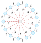
(a)

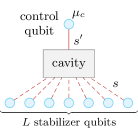
(b)

Figure 1: LABEL:sub@fig:geometry:wheel Lattice geometry of the Bose-Hubbard wheel, see Eq. 1. The $L$ ring sites, each of which is coupled to the center site with an amplitude $s$, exhibit nearest-neighbor hopping with an amplitude $t$. LABEL:sub@fig:geometry:cavity Illustration of the experimental setup based on LABEL:sub@fig:geometry:wheel. The center site couples to an additional lattice site (control qubit) with detuned on-site potential $\mu_{c}$ via an amplitude $s^{\prime}$. In the experimental setup, the center site corresponds to a cavity, the ring sites to SCQs coupled to the cavity.

We consider a Bose-Hubbard model on a wheel geometry in the limit of large interactions $U\rightarrow\infty$, where the bosons become hard-core [34, 32, 33], which will be referred to as BHW in the following. The Hamiltonian of the system is given by (see Fig. 1a)

$$\hat{H}_{\mathrm{wheel}}\equiv-t\sum_{j=0}^{L-1}\left(\hat{h}^{\dagger}_{j}\hat{h}^{\phantom{\dagger}}_{j+1}+\mathrm{h.c.}\right)-\sum_{j=0}^{L-1}\left(s^{\phantom{\dagger}}_{j}\hat{h}^{\dagger}_{j}\hat{h}^{\phantom{\dagger}}_{\odot}+\mathrm{h.c.}\right)\;.$$ (1)

Here, $t$ denotes the hopping on the outer ring of the wheel, consisting of $L$ sites, and $s_{j}=s\mathrm{e}^{\mathrm{i}k_{0}j}$ describes a $k_{0}$-modulated ring-to-center hopping. $\hat{h}^{(\dagger)}_{j}$ corresponds to the hardcore bosons (HCB) annihilation (creation) operator on the $j$-th site of the ring. The index $\odot$ denotes the respective operators on the center site. We consider periodic boundary conditions $\hat{h}^{(\dagger)}_{L}\equiv\hat{h}^{(\dagger)}_{0}$.

In the limit $\frac{s}{t}\rightarrow 0$ (ring geometry), the system exhibits a quasi-Bose-Einstein condensate (BEC) with ground-state occupation $\propto\sqrt{N}$, where $N$ denotes the number of HCB in the system [35, 36, 37, 38]. In the opposite limit $\frac{s}{t}\rightarrow\infty$ (star geometry)[31], the system exhibits a true BEC with ground-state occupation $\propto N$ [39].

In our recent work [34], we solved the full many-body problem of the BHW by mapping the system to a periodic ladder of spinless fermions.

Table 1: Occupations $n_{k_{0}}$ of the $k_{0}$ mode and the corresponding parities $\pi(n_{k_{0}})$.

$n_{k_{0}}$	$0$	$1_{+}$	$1_{-}$	$2$
$\pi(n_{k_{0}})$	even	odd	odd	even

We showed that the many-body spectrum is characterized by an emergent $\mathbb{Z}_{2}$-symmetry, generated by the parity of the distinct $k_{0}$ mode, see table 1, a feature that is inherited from the single-particle dispersion, which we summarize in the following. There are two odd-parity single-particle states, which we label by $n_{k_{0}}=1_{\pm}$. These generate a bulk of many-body energies hosting the BEC -phase, which separate $\propto\pm s\sqrt{L}\equiv\pm\tilde{s}$, referred to as the re-scaled hopping amplitude. This separation of many-body eigenstates $\propto\sqrt{L}$ gives rise to a stabilizing mechanism based on geometric modifications. Furthermore, there are two trivial even-parity states with $n_{k_{0}}=0,2$, which give rise to many-body eigenstates with energies of the order of the band width $t$. From the remaining single-particle eigenstates with $k\neq k_{0}$, a basis of the many-body Hilbert space can be constructed in terms of Slater determinants, which, for the case of $N$ particles, are denoted by $\ket{\mathrm{FS}_{N}}=\ket{\left\{n_{k}\right\}_{k\neq k_{0}}}$ with $n_{k}\in\left\{0,1\right\}$. Crucially, using density-matrix renormalization group (DMRG) the existence of the BEC even in the presence of interactions on the outer ring has been demonstrated [34].

Both the scaling and stability of the many-body gap render the system a promising candidate for a logical qubit architecture. As a brief side remark it should be noted that this implies a possible realization of a BEC using SCQs coupled to a cavity mode. Our subsequent analysis of the stability of the many-body spectrum against experimental imperfections indeed suggests, that for temperatures between $10-100\,\mathrm{mK}$ a BEC could be realized and studied using SCQs.

III The Bose-Hubbard wheel in the presence of noise

Implementing the BHW via SCQs that are coupled to a cavity necessarily generates imperfections, which translate into perturbations of the couplings. The robustness of the BEC against perturbations on the outer ring has been demonstrated previously [34] and is generated from the non-local coupling between the $k_{0}$-mode and the center site. Nevertheless, imperfections can also affect the ring-to-center hoppings $s_{j}$, which are crucial for the formation of the many-body gap separating the BEC states from the trivial ones. To model these imperfections, we consider the effect of perturbations $\delta s_{j}$ to the ring-to-center hopping amplitudes

$$s_{j}=s\mathrm{e}^{\mathrm{i}k_{0}j}\rightarrow(s+\delta s_{j})\mathrm{e}^{\mathrm{i}k_{0}j}\;.$$ (2)

The perturbations $\delta s_{j}$ are modeled by normal distributed, independent, random variables, i.e., $\delta s_{j}\sim\mathcal{N}(0,\sigma^{2})$ with standard deviation $\sigma$. Random realizations of the couplings $s_{j}$ in general break the rotational invariance of the unperturbed BHW Hamiltonian such that a closed solution of the eigenvalue problem does not exist. However, bounds on the induced shifts of the single-particle spectrum can be derived. In particular, for the marginal single-particle eigenvalues $E_{\pm}$, which separate $\propto\tilde{s}$ from the bulk spectrum in the unperturbed case, the eigenvalue equation can be reformulated as a self-consistent problem in terms of the perturbations $\delta s_{j}$. The solution to this eigenvalue problem can be bounded and it is possible to perform the average over the normal distributed perturbations.

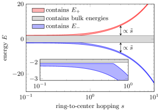
Figure 2: Established bounds for the single-particle spectrum of the perturbed BHW. The displayed data corresponds to $N=1$ particle in a system with $L=6$ ring sites, $k_{0}=\pi/3$ and random coefficients $\delta s_{j}$ with standard deviation $\sigma/t=0.4$. The marginal single-particle energy $E_{+}$ ($E_{-}$) is contained in the red (blue) shaded area, which separates $\propto\tilde{s}$, where $\tilde{s}$ denotes the re-scaled hopping amplitude. All remaining energies are confined to the grey bulk, i.e., to $]-2t,2t[$, characterized by the hopping on the outer ring.

We found that the marginal energies $E_{\pm}$ are only weakly perturbed. For an example realization of the noisy BHW, the single-particle spectrum is shown in Fig. 2. The derived bounds on the marginal energies $E_{\pm}$, see [40], span the blue and red shaded regions separating from the bulk spectrum $\propto\tilde{s}$ and demonstrate the stability of the single-particle gap against perturbations, here at the example of a disorder realization with standard deviation $\sigma/t=0.4$. Expanding the self-consistency equation to first order in the perturbations $\delta s_{j}$, the single-particle eigenvalues $\tilde{E}_{\pm}$ can be averaged over the disorder realizations and we obtain the expectation value of the separating energies

$$\mathrm{E}\left[\tilde{E}_{\pm}\right]=-t\cos{k_{0}}\pm\sqrt{(t\cos{k_{0}})^{2}+\tilde{s}^{2}}+\mathcal{O}(\sigma^{2}/s)\;.$$ (3)

Notably, up to second order corrections in $\sigma$ this is exactly the form of the unperturbed marginal energies, i.e., they coincide with the single-particle energies of the $k_{0}$ mode [34]. Therefore, we conclude that the crucial propery of the BHW, i.e., the separation of two single-particle eigenstates $\propto\pm\tilde{s}$ is also robust against small, random perturbations of the ring-to-center hopping $s$.

Given the robustness of the single-particle spectrum, it is natural to expect that the relevant features of the many-body spectrum of the BHW are stable against random perturbations of the ring-to-center hoppings, too. In the limit of small imperfections $\delta s_{j}\ll\tilde{s}$, we can make this statement more precise by treating $\delta s_{j}$ in perturbation theory. For that purpose, we decompose the perturbed Hamiltonian

$$\hat{H}_{\text{wheel}}^{\text{noise}}=\hat{H}_{\text{wheel}}+\frac{1}{\sqrt{L}}\hat{V}\;,$$ (4)

where we collect all terms containing the perturbations $\delta s_{j}$ in $\hat{V}$. In first order perturbation theory, the corrections of the many-body energies $\Delta E^{\mathrm{noise}}$ can be averaged and we find a quick convergence towards the unperturbed case

$$\Delta E^{\mathrm{noise}}\sim\mathcal{O}(L^{-3/2})\;.$$ (5)

For the many-body energies $E^{\mathrm{noise}}_{\pm}$ separating into an upper and lower branch and, in the unperturbed case, corresponding to the BEC states, we furthermore evaluated the variance of the corrections from first order perturbation theory,

$$\mathrm{Var}\left[\Delta E^{\mathrm{noise}}_{\pm}\right]=c_{\pm}\sigma^{2}+\mathcal{O}(L^{-2})\;,$$ (6)

where the $c_{\pm}$ are constants that do not depend on $\sigma$. A more detailed derivation can be found in [40].

This is one key result of our work: The extensively scaling gap in the many-body spectrum between trivial and BEC states is robust also in the presence of random perturbations $\delta s_{j}$ of the ring-to-center hopping, as long as $\delta s_{j}\ll\tilde{s}$. We want to stress that this result is far from being trivial, because the number of perturbations $\delta s_{j}$ of the system’s Hamiltonian scales with the number of lattice sites $L$ on the outer ring. However, the robustness can be understood by noting that under the Jordan-Wigner transformation, many-particle eigenstates of the BHW Eq. 1 are described by Slater determinants $\ket{FS_{\mathrm{N}}}=\ket{\left\{n_{k}\right\}_{k\neq k_{0}}}$ of single-particle modes  [34]. In the presence of disorder, these Slater determinants are constructed from single-particle eigenstates whose energies are shifted by random perturbations $E\rightarrow E+\delta E$. In leading order, the distribution of the $\delta E$ is dominated by the normal distributed perturbations $\delta s_{j}$. The total contribution of these perturbed Slater determinants to the many-body energies is obtained by summing over all occupied single-particle states, which effectively constitutes an average over the random perturbations $\delta E$ and, thus, the perturbations average out with standard deviation $\sim\sigma$. Importantly, this conclusion can be applied to random variations of the stabilizer qubit frequencies, too. While the separation of the many-body clusters has been shown to be robust under local perturbation on the stabilizer qubits [34], such frequency variations would furthermore detune the stabilizer qubits from the cavity and thereby induce off-resonant couplings to the cavity. For that case, our results can be used to estimate the acceptable imperfections of the stabilizer qubit frequencies such that, given an actual practical realization, the condition $\delta s_{j}\ll\tilde{s}$ can be satisfied.

IV The Bose-Hubbard wheel with a control qubit

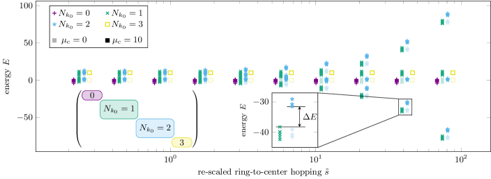
(a)

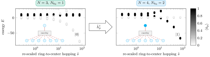
(b)

Figure 3: Many-body spectrum of the wheel-probe system Eq. 7 as a function of the re-scaled hopping amplitude $\tilde{s}$. LABEL:sub@fig:many_body_spectrum Many-body spectrum for $L=6$ ring sites, $N=3$ particles and chemical potentials $\mu_{c}=10$ (bold) and $\mu_{c}=0$ (shaded), as well as control-qubit-to-center hopping $s^{\prime}=0.01$ and outer ring hopping $t=1$. The points mark energies of many-body eigenstates and the color coding denotes their $\hat{N}_{k_{0}}$ sectors. For clarity, for a given value of $\tilde{s}$, the energies for different $N_{k_{0}}$ sectors are plotted next to each other, resulting in spread-out clusters along the $\tilde{s}$ axis. Note that only the energies corresponding to the $N_{k_{0}}=1,2$ sectors gap out for large values of $\tilde{s}$. For a given $\tilde{s}$, different points correspond to the possible configurations $\ket{\mathrm{FS}_{N-N_{k_{0}}}}$ for fixed $L,N$ and $N_{k_{0}}$. The left inset illustrates the block-diagonal matrix structure of the reduced eigenvalue problem for a given $N$-particle sector. The right inset depicts the energy gap $\Delta E$ between the $N_{k_{0}}=1$ and $N_{k_{0}}=2$ sector introduced by the on-site potential $\mu_{c}$ on the control qubit. This establishes the foundation of the effective two-level system, where $\Delta E$ suffices as a lower bound for the gap. LABEL:sub@fig:many_body_spectrum_occupancies shows the lower part of the many-body spectrum for $\mu_{c}=10,L=6$ where $N_{k_{0}}=1$ for $N=3$ (left panel) and $N_{k_{0}}=2$ for $N=4$ (right panel). The color coding denotes the expected probe-site occupation $\braket{\hat{n}_{c}}$. We compare the readout accuracy, i.e., the expected occupation of the control qubit $\braket{\hat{n}_{c}}\approx 0(1)$ in the lower (central) branch in the $N_{k_{0}}=1$ sector (left panel) to the readout accuracy $\braket{\hat{n}_{c}}\approx 1(0)$ in the $N_{k_{0}}=2$ sector (right panel). This defines the effective two-level system. By performing an excitation on the control qubit it is possible to switch between states in both sectors, i.e., $\ket{E_{0}(N,N_{k_{0}}=1)}\rightarrow\ket{E_{0}(N+1,N_{k_{0}}=2)}$. The readout accuracy can be controlled by tuning $\nicefrac{{s^{\prime}}}{{\tilde{s}}}$.

A necessary requirement for an actual use case of the BHW as logical qubit is the ability to store, read out and switch the qubit’s state. Therefore, we modify the setup introducing an additional control qubit that couples to the cavity only, see Fig. 1b. The Hamiltonian then reads

$$\hat{H}_{\mathrm{qubit}}=\hat{H}_{\mathrm{wheel}}+s^{\prime}\left(\hat{h}^{\dagger}_{\odot}\hat{h}^{\phantom{\dagger}}_{c}+\mathrm{h.c.}\right)+\mu^{\phantom{\dagger}}_{c}\hat{n}^{\phantom{\dagger}}_{c}\;,$$ (7)

where $\hat{h}^{(\dagger)}_{c}$ denotes annihilation (creation) operator for the additional control qubit, $\hat{n}^{\phantom{\dagger}}_{c}=\hat{h}^{\dagger}_{c}\hat{h}^{\phantom{\dagger}}_{c}$, and $\mu^{\phantom{\dagger}}_{c}$ a chemical potential. It is worth mentioning that in the following we consider the general case of a finite hopping amplitude $t$, which we choose as unit of energy. Then, the width of the clusters in the many-body spectrum is given by $2t$ [34]. Upon introducing the control qubit, a second cluster of odd-parity eigenstates is generated and the corresponding, energetically low-lying many-body eigenstates can be separated from the remaining spectrum by geometric stabilization, increasing $\tilde{s}$. Notably, the resulting two clusters are composed of many-body eigenstates that break particle-number conservation on the outer ring of the wheel and realize BECs that can be distinguished by their constituting Slater determinants [34]. Thus, local perturbations, acting on the $L$ stabilizer qubits (the wheel’s outer ring) couple many-body eigenstates within the same cluster. This gives rise to a redundancy of the represented logical qubit state, which scales exponentially in $L$.

For the solution of the many-body problem we introduce $\hat{N}_{k_{0}}=\hat{n}_{c}+\hat{n}_{k_{0}}$, the sum of the occupation of the $k_{0}$ mode and the control qubit. From the conservation of $\hat{N}_{k_{0}}$ it follows that for a given, Jordan-Wiger transformed, Slater determinant $\ket{\mathrm{FS}_{N}}$ of $N$ single-particle eigenstates, Eq. 7, decomposes into a block-diagonal representation $\braket{\mathrm{FS}_{N}}{\hat{H}_{\mathrm{qubit}}}{\mathrm{FS}_{N}}=\bigoplus_{N_{k_{0}}}\hat{h}(\mathrm{FS}_{N},N_{k_{0}})$. The individual block dimensions are given by

$$d_{N_{k_{0}}}=\operatorname{dim}[\hat{h}(\mathrm{FS}_{N},N_{k_{0}})]=\begin{cases}1,&\text{if $N_{k_{0}}=0,3$,}\\ 3,&\text{if $N_{k_{0}}=1,2$,}\end{cases}$$ (8)

and the remaining eigenvalue problem of Eq. 7 can be solved in each block, individually. To explicitly account for the conservation of the overall particle number, $N$, we re-sort the blocks and group together those with the same total number of occupied modes in the Slater determinants and the $N_{k_{0}}$ sector, i.e., we fix $N$ and obtain a block for each $N_{k_{0}}$ with $N-N_{k_{0}}$ occupied modes in the Slater determinants, see inset of Fig. 3a. In this basis, eigenstates can be represented by

$$\ket{E_{\nu}(N,N_{k_{0}})}=\ket{\nu_{N_{k_{0}}}}\otimes\ket{\mathrm{FS}_{N-N_{k_{0}}}}\;,$$ (9)

where $\nu_{N_{k_{0}}}=0,\dots,d_{N_{k_{0}}}-1$ labels the eigenstates in the corresponding $N_{k_{0}}$-sectors sorted by their energies. While the full solution strategy for the eigenvalue problem of Eq. 7 is given in [40], here, we will focus on the relevant part of the many-body spectrum.

IV.1 Logical qubit and $X$-gate implementation

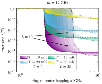
(a)

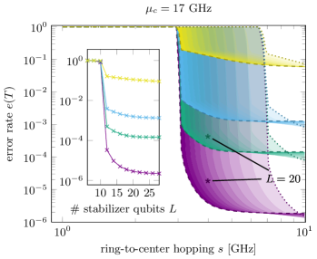
(b)

Figure 4: Error rate $e(T)$ as a function of the ring-to-center hopping amplitude $s$ for different temperatures $T=10,15,20,50\,\mathrm{mK}$ and $\mu_{c}=12,17$ at fixed probe-to-center hopping $s^{\prime}=0.01$ and outer-ring hopping $t=1$. The shaded areas are spanned by the values of $e(T)$ at fixed $T$ for different numbers of stabilizer qubits $L=6,\ldots,28$. The smallest (largest) $L=6(28)$ are denoted by the dashed (dotted) lines and the fill color saturation indicates the intermediate values. For $s<s_{c}(T,L)$, where $s_{c}(T,L)$ denotes a temperature-and system-size dependent critical value of $s$, increasing the amount of stabilizer qubits $L$ results in a lower error rate where the improvement becomes significant in the low-temperature regime $T<50\,\mathrm{mK}$. For $s>s_{c}(T)$, this behavior is reversed and adding more stabilizer qubits does not improve the error rate. The effect of geometric stabilization is to reduce the coupling strength $s$ between stabilizer qubits and cavity, in order to achieve a certain error rate. This is illustrated in the inset, where we show the error rate as a function of $L$ for a fixed value of $s=5\,\mathrm{GHz}$, which is at the upper limit of practically doable couplings [41].

To realize an effective two-level system, there are two symmetry sectors of particular interest, namely $\hat{N}_{k_{0}}=1$ and $\hat{N}_{k_{0}}=2$ with block dimension $d_{N_{k_{0}}}=3$, each. To understand the effect of the control qubit on the unperturbed wheel’s eigenstates we can treat $s^{\prime}/\tilde{s}$ as a small perturbation. This is motivated by the fact that in practical realizations $\tilde{s}$ should be as large as possible to stabilize the non-trivial BEC phase.

Then, the first non-vanishing corrections appear in second order, i.e., the structure of the many-body spectrum of the unperturbed wheel is reproduced in the two relevant $N_{k_{0}}$ sectors with corrections $\sim\mathcal{O}((\nicefrac{{s^{\prime}}}{{\tilde{s}}})^{2})$. An example for the many-body spectrum as a function of $\tilde{s}$ is shown in Fig. 3a for $s^{\prime}=1$. Fig. 3b shows the control qubit occupation indicated by the fill color in each many-body eigenstate of the $N_{k_{0}}=1$ (left) and $N_{k_{0}}=2$ (right) sector. Evaluating the occupation of the control qubit for the eigenstates corresponding to the lower branch of the spectrum using perturbation theory, yields

$$\braket{\hat{n}_{c}}_{N_{k_{0}}=1}=\mathcal{O}\left(\left(\frac{s^{\prime}}{\tilde{s}}\right)^{2}\right)\;,\\ \braket{\hat{n}_{c}}_{N_{k_{0}}=2}=1-\mathcal{O}\left(\left(\frac{s^{\prime}}{\tilde{s}}\right)^{2}\right)\;.$$ (10)

Note that increasing $\tilde{s}$, the occupations quickly saturate to either $\braket{\hat{n}_{c}}=0$ or $\braket{\hat{n}_{c}}=1$, depending on the respective symmetry sector. This defines an effective two-level system between states in the two $N_{k_{0}}$ clusters

$$\ket{0}\stackrel{{\scriptstyle\sim}}{{=}}\ket{\nu_{N_{k_{0}}=1}}\;,\quad\ket{1}\stackrel{{\scriptstyle\sim}}{{=}}\ket{\nu_{N_{k_{0}}=2}}\;,$$ (11)

for which the readout accuracy can be controlled by tuning $s^{\prime}/\tilde{s}$.

In the limit $t=0$, i.e., the star geometry, the energies corresponding to different configurations within a given $N_{k_{0}}$ sector reduce to a single value, which allows us to define the energy gap of the logical qubit as

$$\Delta E=E_{2}-E_{1}\propto\mu_{c}\;,$$ (12)

with

$$E_{1}=E_{0}(N,1)\quad\text{and}\quad E_{2}=E_{0}(N+1,2)\;.$$ (13)

This gap can be controlled by the chemical potential $\mu_{c}$ on the control qubit. Importantly, $\mu_{c}$ has no effect on the corrections of the probe-site occupations such that it can be treated as a free parameter that can be chosen as large as experimentally possible. For a fixed coupling $s^{\prime}/t=1$, we indeed find a linear relation between $dE$ and the chemical potential $\mu_{c}$, see [40]. In our specific setup, $\mu_{c}$ can be controlled by the frequency detuning of the control qubit compared to the stabilizer qubits. Since the proposed logical qubit does not require gate operations on the stabilizer qubits, the frequencies of the stabilizer qubits may be increased beyond the adressable regime, allowing even larger detunings between the stabilizer qubits and the control qubit. For instance, typical frequencies for adressable transmon qubits range between $1\,\mathrm{GHz}-10\,\mathrm{GHz}$, but this range can be increased to $100\,\mathrm{GHz}$ if no gate operations are required. This should be compared to anharmonicities in current transmons, which are of the order of $100\,\mathrm{MHz}$ [30, 42].

We now consider a finite-temperature representation of the ground state $\ket{0}$ of the logical qubit where the quality is controlled by the interplay of the different paramters $t,s,\mu_{s}$ and $s^{\prime}$. The thermal density operator is given by

$$\hat{\rho}_{0}(T)=\frac{1}{Z}e^{-\beta\hat{H}_{\mathrm{qubit}}}\;,$$ (14)

where $\beta=1/k_{B}T$, $k_{B}$ denotes the Boltzmann constant, and $Z$ the partition function. We define the fidelity of the $X$-gate as the probability to find the control qubit in a $\ket{1}$ state after performing the excitation

$$\hat{\rho}_{0}(T)\mapsto\hat{c}^{\dagger}_{p}\hat{\rho}_{0}(T)\hat{c}^{\phantom{\dagger}}_{p}=\hat{\rho}_{1}(T)\;,$$ (15)

as function of T. This can be evaluated by performing the partial trace over the excited state projected into the lower branch of the $N_{k_{0}}=2$ sector

$$F(T,N)\equiv\sum_{\left\{\mathrm{FS}_{N-2}\right\}}\bra{E_{0}(N+1,2)}\hat{\rho}_{1}(T)\ket{E_{0}(N+1,2)}\;,$$ (16)

where the sum is over all Slater determinants with $N-2$ modes occupied. In the following, we choose a practically relevant energy scale, i.e., typically transmon frequencies $\omega=1\,\mathrm{GHz}$ as unit of energy.

From the fidelity, we immediately get the error rate for switching the state of a single qubit, which is of fundamental importance. It constitutes a lower bound for the error rate of two-site gate operations and controls the approximation quality of quantum algorithms. We define $e(T)$ as the probability of finding our qubit in an eigenstate, which is not in the targeted lower $N_{k_{0}}=2$ branch: $e(T)=1-F(T)$. In Fig. 4 we show $e(T)$ for different temperatures at half filling $N=L/2$ as a function of $s$ and detunings $\mu_{c}=12,17\,\mathrm{GHz}$. The shaded areas are spanned by the values of $e(T)$ for different numbers of stabilizer qubits $L=6,\dots,28$, where the dashed (dotted) boundaries correspond to $L=6(28)$ and the fill color saturates with increasing $L$. For a fixed temperature and detuning, the dominating control parameter of the error rate is $s$ and we observe a steep decrease towards a lower bound set by the ratio $\mu_{c}/T$. The origin of this sharp drop is the separation of the lower $N_{k_{0}}=1,2$ clusters from the central clusters in the many-body spectrum and signals the separation of the two logical qubit states. The width of the shaded areas is controlled by the relation between that separation and the rescaled coupling $\tilde{s}=s\sqrt{L}$.

For sufficiently large values of $s$, details of the many-body spectrum such as the number of eigenstates per $N_{k_{0}}$ sector become relevant. The onset of this regime of the ring-to-center hopping is indicated by the crossing points in the shaded areas, $s=s_{c}(T)$. As long as $s<s_{c}(T)$, the error rate can be reduced significantly by increasing the wheel’s coordination number $L$, in particular at low temperatures $T<50\,\mathrm{mK}$. In this case, the crossing point $s_{c}(T)\sim 10\,\mathrm{GHz}$ would be hard, if not impossible, to reach in experiment. Here, the importance of the wheel geometry becomes apparent: In order to achieve large fidelities (small error rates), the geometric stabilizing mechanism of the BHW with an extensively scaling many-body gap is the key feature. Within the presented calculations single qubit-gate fidelities of $F>0.999$ can be reached by coupling $L=20$ qubits to a cavity at a temperature of $15\,\mathrm{mK}$.

IV.2 Measuring the qubit state

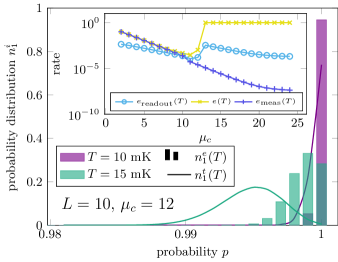
(a)

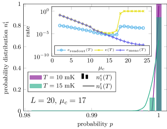
(b)

Figure 5: Comparison of theoretical and experimental probability distribution for coupling strength between stabilizer qubits and cavity $s=4$, $s^{\prime}=0.01$ and $t=1$. We show data for $L=10(20)$ stabilizer qubits with detunings $\mu_{c}=12(17)$ in Fig. 5a (Fig. 5b) at half filling for $T=10,15\,\mathrm{mK}$. The bar plots show the experimental probability distribution to obtain an occupied control qubit from the simulated measurement of the control qubit, $n_{1}^{e}$, in a sequence of $M=10^{3}$ independent excitation processes and averaged over an ensemble of $K=10^{3}$ independent realizations. The line plots correspond to the theoretical probability distribution $n_{1}^{t}(T)=B(M,p=F(T))$. The inset shows the theoretical error rate $e(T)$ (yellow curve) as well as the experimental error rate $e_{\mathrm{meas}}(T)$ (dark blue curve) as a function of the on site potential of the control qubit $\mu_{c}$. The geometric mean of both curves, $e_{\mathrm{readout}}$ (light blue curve), suffices as a calibration function. Minimizing this curve leads to the optimal value of the detuning $\mu_{c}$.

In the previous analysis it was assumed that the fidelity of an excitation of the logical qubit can be identified by determing the weight of the $\ket{1}$ states in the post-excitation density operator. However, in practise one measures the occupation of the control qubit after an excitation (see Fig. 3b). We identify states in the lower branch of the $N_{k_{0}}=2$ sector via an occupied control qubit, and thereby verify if an excitation on the control qubit has successfully created the excited state $\ket{1}$ of the logical qubit. However, there can be false positives, i.e., the control qubit can be occupied although the corresponding eigenstate is not in the desired lower branch of the $N_{k_{0}}=2$ sector.

To deduce the impact of these false positives, we compare the theoretically obtained probability distribution to find a state in the desired low-lying $N_{k_{0}}=2$ sector to the probability distribution to measure an occupied control qubit. The theoretical distribution is given by a binomial distribution characterized by the fidelity $n_{1}^{t}(T)=B(M,p=F(T))$, with $F(T)$ defined in Eq. 16 and $M$ being the number of trials. To obtain the experimentally accessible probability distribution, we simulate a sequence of $M$ independent measurement processes on the thermal density operator $\hat{\rho}_{1}(T)$ at different temperatures $T$, yielding $N_{1}(T)\leq M$ cases of occupied control qubits. Averaging $N_{1}(T)$ over an ensemble of $K$ independent realizations provides access to the experimentally observed distribution of the relative incidences $n^{e}_{1}(T)=N_{1}(T)/M$.

Fig. 5 compares the experimental and theoretical distribution for temperatures $T=10,15\,\mathrm{mK}$ and $L=10(20)$ stabilizer qubits at detunings $\mu_{c}=12(17)$. For $L=10$, see Fig. 5a, the impact of false positives can be observed clearly as a shift of the mean towards higher incidences, compared to the theoretical distribution. For the smallest temperature considered ($T=10\,\mathrm{mK}$), the experimentally observable fidelity overestimates the actual fidelity to excite into the desired $N_{k_{0}}=2$ branch by approximately $3$ out of $1000$ samples. Increasing $L$ to $L=20$ allows to obtain better agreement of both distributions, see Fig. 5b. Again, this can be explained by geometric stabilization, which allows to suppress the effect of false positives caused by states in other clusters. To further increase the agreement, it is possible to choose $\mu_{c}$ in an optimal way by minimizing the calibration function

$$e_{\mathrm{readout}}(T)=\sqrt{\absolutevalue{e(T)-e_{\mathrm{meas}}(T)}\cdot e(T)}\;.$$ (17)

Here, $e(T)=1-F(T)$ denotes the theoretical error rate and $e_{\mathrm{meas}}(T)$ the experimental error rate, i.e., the probability of the control qubit not being occupied in a measurement. We defined the calibration function as the geometric mean of both rates. As a key result, we observe that for the optimal detuning $\mu_{c}\approx 17$, error rates $e<10^{-3}$ can be obtained, which is shown in the insets of Fig. 5. Note that in these computations we neglected the impact of noisy wheel-to-center couplings, which is justified by the results in Sec. III, showing that for practical realizations the modifications of the many-body spectrum are irrelevant compared to the energy shifts introduced from geometrical stabilization.

V Conclusion and Outlook

We proposed a logical qubit construction scheme based on the peculiar property of the BHW (in the infinite-$U$ limit) to open a gap between clusters of many-body eigenstates with the energetically lowest states exhibiting Bose-Einstein condensation [34]. Exploiting the fact that this gap scales $\propto\sqrt{L}$ where $L$ is the number of lattice sites on the outer ring, i.e., the coordination number, we suggest a setup for the logical qubit in which these hardcore-bosonic sites are realized by SC stabilizer qubits, and the all-to-one coupling to the wheel’s center site is implemented by resonantly coupling the qubits to a cavity mode. This way, the energetically low-lying cluster of many-body eigenstates of the BHW can be separated from the remaining part of the spectrum by increasing the number of stabilizer qubits. For the resulting architecture, we investigated the robusteness of the separation of this cluster in the presence of disorder to evaluate the effect of experimental imperfections. We derived bounds on the induced perturbations under the assumption that the couplings between the qubits and the cavity mode are subject to normal distributed imperfections and showed that corrections to the gap-opening are occurring only in second order in the standard deviation $\sigma$. Taking into account the robustness of the BHW against local perturbation on the outer ring (the stabilizer qubits), we expect the logical qubit setup to be remarkably stable against fabrication errors. Importantly, this also includes imperfections of the stabilizer qubits frequencies, which translate into random disorder potentials in Eq. 7 and off-resonant couplings to the cavity.

Introducing an additional, frequency-detuned control qubit, which is only coupled to the cavity, we showed that an effective two-level system composed of clustered many-body eigenstates emerges, which is separated form the bulk states by the wheel’s many-body gap. The two clusters of low-energy states can be separated by detuning the frequencies of the control qubit w.r.t. stabilizer qubits. The resulting logical qubit can be read out and switched via local operations on the control qubit, only. For a single-qubit $X$-gate acting on the logical ground state, we computed the fidelity $F(T)$ and showed that for experimentally feasible transmon frequencies, temperatures $T\sim 15\,\mathrm{mK}$ are sufficient to reach theoretical error rates $e(T)=10^{-4}$, using $L=20$ stabilizer qubits. In these calculations, the relevant quantity is the ratio between the renormalized coupling $\tilde{s}$ of the stabilizer-qubits to the cavity and the frequency detuning between stabilizer qubits and control qubit $\mu_{c}$. This can be exploited to adopt to practical constraints, for instance a reduction of the cavity frequency when increasing its length in order to increase the number of stabilizer qubits. We also analyzed the occurrence of read-out errors (false positives) and introduced a calibration function, which can be used to experimentally vary the detuning such that the combined false-positive- and theoretical error-rate is minimized. Given a certain number of stabilizer qubits, the calibration function therefore allows to tune the logical qubit such that for the discussed parameters ($L=20$, $T=15\,\mathrm{mK}$), it can be operated with minimal error rates $<10^{-4}$ using a frequency detuning of the probe-site qubit of $\approx 17\,\mathrm{GHz}$.

Our analysis of the robustness of the presented logical qubit suggests a high degree of control to suppress the effects of perturbations introduced by experimental imperfections and temperature. Nevertheless, our considerations are based on two critical assumptions: (i) the constituting SCQs are ideal two-level systems and (ii) there is only one excitation in the cavity at the most. For weak violations of the first assumption, i.e., a small subset of the stabilizer qubits forming the wheel exhibit a loss of coherence or excitations into energetically higher states, we still expect our results to be valid. This is based on the fact that the logical qubit-state is encoded with a high redundancy in a cluster of many-body eigenstates whose number scales exponentially with the wheel’s coordination number. The second assumption could be realized to a very high degree via fine-tuning the stabilizer qubits to resonance with the cavity and choose a large qubit frequency, compared to the qubit-to-cavity coupling strength $s$. However, further theoretical and numerical work is required to validate these assumptions and to investigate the impact of violations. For instance, for case (i) effects of the anharmonic transmon spectrum could be studied numerically using open quantum-system methods, while case (ii) suggests simulations with a bosonic center site. A further practical source of imperfections that needs to be considered is the quality factor of the cavity. We nevertheless expect that the presented results will motivate experimental realizations, beginning with the wheel geometry itself to realize Bose-Einstein condensates at temperatures in the range of $10-20\,\mathrm{mK}$, and subsequently the implementation of the logical qubit.

Supplemental Materials

VI Solution Strategy of the Bose-Hubbard wheel

The Hamiltonian of the Bose-Hubbard wheel is given by

$$\hat{H}_{\mathrm{wheel}}=-t\sum_{j=0}^{L-1}\left(\hat{h}^{\dagger}_{j}\hat{h}^{\phantom{\dagger}}_{j+1}+\mathrm{h.c.}\right)-\sum_{j=0}^{L-1}\left(s_{j}\hat{h}^{\dagger}_{j}\hat{h}^{\phantom{\dagger}}_{\odot}+\mathrm{h.c.}\right)\;,$$ (S1)

where $\hat{h}^{(\dagger)}_{j}$ denote the hardcore bosonic annihilation (creation) operators on site $j$ on the ring of the wheel while $\hat{h}^{(\dagger)}_{\odot}$ corresponds to the annihilation (creation) of HCB on the center site. $L$ denotes the number of sites on the ring and we consider periodic boundary conditions. Direct application of common solution strategies fail due to long-ranged hopping introduced by the center cite when mapping the system to a chain. Our solution strategy is based on a geometric ansatz that maps the Bose-Hubbard wheel to a spinless fermion ladder with periodic boundary conditions. On this extended Hilbert space, the full many-body problem can be solved and eventually projected down to the initial Hilbert space. Please note that a more detailed derivation of the solution strategy can be found in our recent publication [34]. The resulting many-body eigenstates have the structure

$$\ket{n_{k_{0}}}\ket{FS_{N-n_{k_{0}}}}\;,$$ (S2)

where $n_{k_{0}}=0,1_{\pm},2$ denotes the occupation of a distinct mode and the entire many-body problem reduces to the diagonalization of a $4\times 4$ matrix, see left side of Fig. S1.

Figure S1: Blockdiagonal structure of the Hamiltonian in $n_{k_{0}}$ (left, Eq. S1) before and in $N_{k_{0}}$ (right, Eq. S19) after adding the control qubit to the system. The matrix on the right is spanned by all possible combinations of states with occupations $n_{k_{0}}=0,1_{\pm},2$ and $n_{c}=0,1$. Hence, the blocks have the size $1-2-1$ and $1-3-3-1$. To provide an example, in the $N_{k_{0}}=0,3$ subspaces the corresponding states have the form $\ket{n_{c}=0}\ket{n_{k_{0}}=0},\ket{n_{c}=1}\ket{n_{k_{0}}=2}$, respectively.

The occupation of the $k_{0}$ mode has significant effects on both the single-and many-particle spectrum, as it gaps out $\propto s\sqrt{L}$ while all remaining modes follow a common tight-binding dispersion. Furthermore $n_{k_{0}}$ generates a $\mathbb{Z}_{2}$ symmetry in the many-body spectrum distinguishing BEC states, which gap out $\propto s\sqrt{L}$ as a result of this characteristic, and non-BEC states. $\ket{FS_{N-n_{k_{0}}}}$ denotes a Slater determinant of $N-n_{k_{0}}$ $k\neq k_{0}$ modes with $k\in\left\{k_{n}=\frac{2\pi}{L}n|n=0,\ldots,L-1\right\}$.

The eigenstates of the projected wheel are given by

$$\ket{E_{n_{k_{0}}=0}(\mathrm{FS}_{N})}=\ket{0}\ket{FS_{N}}\;,$$ (S3)

$$\ket{E_{n_{k_{0}}=\pm}(\mathrm{FS}_{N-1})}=\ket{\pm}\ket{FS_{N-1}}\;,$$ (S4)

$$\ket{E_{n_{k_{0}}=2}(\mathrm{FS}_{N-2})}=\ket{2}\ket{FS_{N-2}}\;,$$ (S5)

where $\ket{\pm}$ diagonalize the $n_{k_{0}}=1$ subspace. These expressions, as well as the analytically obtained many-particle energies for the $4\times 4$ $n_{k_{0}}$ subspace

$$E_{0}(FS_{N}) =E(FS_{N}),$$ (S6)

$$E_{\pm}(FS_{N-1},k^{\prime}) =E(FS_{N-1})\left(1-\frac{1}{L}\right)+1\pm\sqrt{\left(\frac{E(FS_{N-1})}{L}+1\right)^{2}+\tilde{s}^{2}},$$ (S7)

$$E_{2}(FS_{N-2},k^{\prime},k^{\prime\prime}) =\left(E(FS_{N-2})+2\right)\left(1-\frac{2}{L}\right)\;,$$ (S8)

will be needed for the solution strategy of the wheel-probe system. Here, $k^{\prime},k^{\prime\prime}$ denote the $k_{0}$ modes. Note that these energies depend on the choice of Slater determinant $FS_{N}$ outside of the $n_{k_{0}}$ subspace.
For later convenience, we state the eigenstates $\ket{\pm}$ for a given Slater determinant

$$\ket{\pm}=c^{\pm}_{1+}\ket{1_{+}}+c^{\pm}_{1-}\ket{1_{-}}=d^{\pm}_{0}\ket{n_{k_{0},O}=1}\ket{n_{\odot}=0}+d^{\pm}_{1}\ket{n_{k_{0},O}=0}\ket{n_{\odot}=1}\;,$$ (S9)

where $d^{\pm}_{0}=c^{\pm}_{1+}\psi_{+}+c^{\pm}_{1-}\psi_{-}$ and $d^{\pm}_{1}=c^{\pm}_{1+}\psi_{+}\Delta_{+}+c^{\pm}_{1-}\psi_{-}\Delta_{-}$. Here, $n_{k_{0},O}(n_{\odot})$ denotes the occupation of the $k_{0}$ mode on the outer ring (center site) of the wheel. The coefficients are given by $\psi_{\pm}=\frac{1}{\sqrt{1+\absolutevalue{\Delta_{\pm}}^{2}}}$, $\Delta_{\pm}=\frac{\epsilon_{0}}{2\tilde{s}}\pm\frac{\sqrt{\epsilon^{2}_{0}+4\tilde{s}^{2}}}{2\absolutevalue{\tilde{s}}}$ and $\epsilon_{0}=2t\cos{k_{0}}$. The remaining states take the form

$$\ket{0}=\ket{n_{k_{0},O}=0}\ket{n_{\odot}=0},\ket{2}=\ket{n_{k_{0},O}=1}\ket{n_{\odot}=1}\;.$$ (S10)

VII Noise

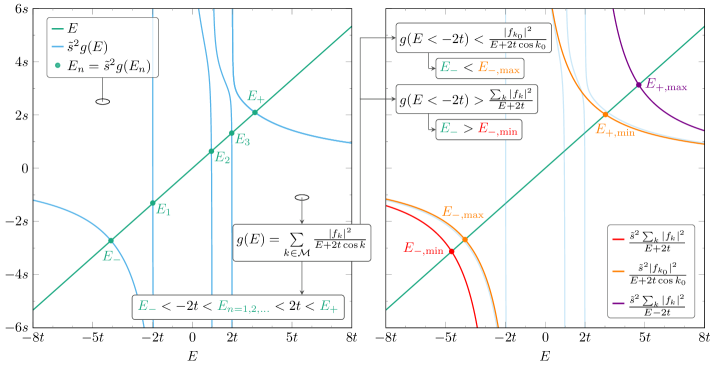
Figure S2: Graphical representation of Eq. (S14) for a system with $L=6$ lattice sites on the outer ring, $k_{0}=\pi/3$, $s/t=1.5$ and random coefficients $s_{j}$ with $\sigma/t=0.4$. The solutions $E_{n}$ are given by the intersections of the blue and green graph in the left panel. The best bounds for $E_{-}$ are obtained from evaluating Eq. S15 at $k=k_{0}$ and solving for the intersections, which are marked by $E_{\mathrm{-,min}}$ and $E_{\mathrm{-,max}}$ in the right panel. Similarly, the corresponding best estimations for the bounds on $E_{+}$ are marked by $E_{\mathrm{+,min}}$ and $E_{\mathrm{+,max}}$.

Here, we outline the analysis of the Bose-Hubbard wheel’s spectrum in the presence of noise in detail. Mapping the hardcore-bosonic operators $\hat{h}^{(\dagger)}_{j},\hat{h}^{(\dagger)}_{\odot}$ to fermionic operators $\hat{c}^{(\dagger)}_{k},\hat{c}^{(\dagger)}_{\odot,k}$, the corresponding Hamiltonian in the periodic-ladder representation [34] is given by $\hat{H}_{\mathrm{wheel}}^{\mathrm{noise}}=\hat{\Pi}_{\odot}\hat{H}_{\mathrm{lad}}^{\mathrm{noise}}\hat{\Pi}_{\odot}$ with

$$\hat{H}_{\mathrm{lad}}^{\mathrm{noise}} =-\sum_{k\in\mathcal{M}}\left[2t\cos(k)\hat{n}_{k}^{\phantom{\dagger}}\left(1-\frac{2}{L}\hat{n}_{\odot,k=0}\right)+\tilde{s}\left(f_{k}^{\phantom{\dagger}}\hat{c}_{k}^{\dagger}\hat{c}_{\odot,k=0}^{\phantom{\dagger}}+\text{h.c.}\right)\right],$$ (S11)

where the sum is over all momenta $k\in\mathcal{M}$. Here, we introduced the Fourier transformed, perturbed ring-to-center hoppings $f_{k}=\delta_{k,k_{0}}+\frac{1}{\sqrt{L}}\sum_{j}(\delta s_{j}/\tilde{s})\mathrm{e}^{\mathrm{i}(k_{0}-k)j}$. Considering an ensemble of wheels, one could immediately evaluate the average of $f_{k}$ using the fact that $\sqrt{\mathrm{Var}[f_{k}]}=\sigma/\tilde{s}$ and $\mathrm{E}[f_{k}]=\delta_{k,k_{0}}$, which implies a quick convergence to the unperturbed system’s spectrum in the limit $\tilde{s}/\sigma\to\infty$. However, in our setup a wheel is supposed to represent a single logical qubit. As a consequence, we have to investigate the spectral properties of Eq. S11 for individual realizations of the imperfections $\delta s_{j}$ at finite $\tilde{s}/\sigma$.

From the analysis of the unperturbed Bose-Hubbard wheel it is known that the single-particle gap controls the separation of the many-particle spectrum into trivial and BEC states. Hence, we start our discussion with an analysis of the perturbed Bose-Hubbard wheel in the single-particle subspace. In that case, exploiting $\hat{n}_{k}\hat{n}_{\odot,k=0}=0$, we can solve Eq. S11 for the single-particle eigenstates, which can be divided into two sets. The first set of eigenstates is characterized by momenta $q\in\{k_{n}\in\mathcal{M}|0<k_{n}<\pi\}\equiv\mathcal{M}^{\prime}$:

$$\hat{\Psi}_{q}^{\dagger}\ket{\varnothing}=d_{q}\left(f^{\ast}_{2\pi-q}\hat{c}_{k}^{\dagger}-f^{\ast}_{k}\hat{c}_{2\pi-q}^{\dagger}\right)\ket{\varnothing}\;,$$ (S12)

with single-particle eigenvalues $E_{q}=-2t\cos{q}\in]-2t,2t[$ and normalization $d_{q}$. For $L$ even (odd), these $|\mathcal{M}^{\prime}|=(L-2)/2$ states ($|\mathcal{M}^{\prime}|=(L-1)/2$ states) represent superpositions of plane waves occurring on the outer ring exclusively and their energies are constrained by the usual tight-binding dispersion relation. The second set of eigenstates non-locally couples excitations on the outer ring with excitations on the inner ring and can be parametrized as

$$\hat{\Psi}_{n}^{\dagger}\ket{\varnothing}=d_{n}\left(\hat{c}_{\odot,k=0}^{\dagger}+\sum_{k\in\mathcal{M}}b_{n,k}\hat{c}_{k}^{\dagger}\right)\ket{\varnothing}\;.$$ (S13)

Here, the parameters $b_{n,k}=-\tilde{s}f_{k}/(E_{n}+2t\cos k)$ need to be determined from solving a self-consistent equation for the corresponding single-particle eigenvalues

$$E_{n}=\tilde{s}^{2}\sum_{k\in\mathcal{M}}\frac{|f_{k}|^{2}}{E_{n}+2t\cos{k}}\equiv\tilde{s}^{2}g(E_{n})\;.$$ (S14)

Even though this equation does not allow for an analytic solution, it is possible to gain further insights by closer analyzing the function $g(E)$. Its domain consists of the set of disjoint intervals $\mathcal{I}_{n}=]-2t\cos{k_{n}},-2t\cos{k_{n+1}}[$ and the two marginal intervals $\mathcal{I}_{-}=]-\infty,-2t[$ and $\mathcal{I}_{+}=]2t,\infty[$. In each interval, $g(E)$ is continuous and strictly decreasing with poles located at the boundaries, which are given by the tight-binding eigenvalues $E_{n}=-2t\cos k_{n}$. To illustrate the structure of $g(E)$, in Fig. S2 we show a realization for a certain choice of perturbations $\delta s_{j}$ and $L=6$ sites on the outer ring. The branches of $g(E)$ in the intervals $\mathcal{I}_{n},\mathcal{I}_{\pm}$ are shown by the blue lines. The solutions to Eq. S14 are located at the intersections between the function $y(E)=E$, i.e., the main diagonal in Fig. S2 plotted as green line, and $\tilde{s}^{2}g(E)$. They are marked as green dots, shown in the left panel. Since both functions, $y(E)$ and $g(E)$, are strictly increasing and decreasing in every interval, respectively, there are unique solutions $E_{n}\in\mathcal{I}_{n}$ and $E_{\pm}\in\mathcal{I}_{\pm}$, i.e., for $L$ even (odd), there are $(L+4)/2$ eigenvalues ($(L+3)/2$ eigenvalues) contributed from the second set of Eigenstates, which confirms that the single-particle problem is indeed solved completely by determining the solutions $E_{n}$ to Eq. S14.

The marginal energies $E_{\pm}$ are of primary interest because they determine the size of the single-particle gaps. For that reason, we establish an upper bound for the solution $E_{n}=\tilde{s}^{2}g(E_{n})$ with $E_{n}<-2t$ by estimating $g(E_{n})<|f_{k}|^{2}/(E_{n}+2t\cos{k})$ for all $k\in\mathcal{M}$. Similarly, a lower bound can be introduced via $g(E_{n})>\sum_{k\in\mathcal{M}}|f_{k}|^{2}/(E_{n}+2t)$, yielding bounds for the lower marginal energy

$$E_{-}<-t\cos{k}-\sqrt{(t\cos{k})^{2}+\tilde{s}^{2}|f_{k}|^{2}}\;,$$ (S15)

for all $k\in\mathcal{M}$ and

$$E_{-}>-|t|-\sqrt{t^{2}+\tilde{s}^{2}\sum_{k\in\mathcal{M}}|f_{k}|^{2}}\;.$$ (S16)

The bounds on $\tilde{s}^{2}g(E_{-})$ and $E_{-}$ are shown in the right panel of Fig. S2 where we evaluated the upper bound at $k=k_{0}$, yielding the best approximation. Accordingly, the marginal single-particle energy $E_{+}$ can be bounded and we show the resulting best bounds in the right panel of Fig. S2. An important result of these estimations is that the marginal energies $E_{\pm}$ are gaped out from the bulk of the single-particle spectrum $\propto\lvert\tilde{s}f_{k_{0}}\rvert$.

Figure S3: Distributions of the marginal energies $E_{\pm}$ for $10^{4}$ independent realizations $\left\{\delta s_{j}\right\}$ of the Bose-Hubbard wheel with $L=6$ lattice sites on the outer ring, $k_{0}=\pi/3$, $s/t=1.5$ and random imperfections $\delta s_{j}$ with $\sigma/t=0.01$. The sample-means for the single-particle eigenvalues $E_{+}$ ($E_{-}$) are represented by the red (blue) dashed lines. The solid lines indicate the marginal single-particle eigenvalues of the unperturbed system separating from the bulk spectrum $\propto\tilde{s}$. The means of the perturbed and the unperturbed marginal energies are nearly on top of each other (we show an enlarged excerpt in the insets), even for the rather moderate choices of the ring-to-center hopping and the width of the distribution of the imperfections.

The established bounds on the marginal single-particle energies explicitely depend on the realization of the perturbed ring-to-center hoppings $s+\delta s_{j}$ via $f_{k}$. Thus, controlling the width $\sigma$ of the distribution of the imperfections $\delta s_{j}$ is important. A justification for assuming $\sigma/s\ll 1$ is provided in VII.1. We statistically analyze $E_{\pm}$ neglecting quadratic and higher orders in $\delta s_{j}$ on the right-hand side of Eq. S14. Thereby, we obtain two solutions $\tilde{E}_{\pm}$, which fulfill the self-consistency condition up to quadratic order in $\sigma$, yielding expectation values given in Eq. 3, which correspond to the marginal single-particle energies of the isotropic Bose-Hubbard wheel. Furthermore, the variance can be computed in this approximation, yielding $\mathrm{Var}[\tilde{E}_{\pm}]\in\mathcal{O}(\sigma^{2})$. Evaluating the boundaries’ variances from Eqs. S15 and S16 directly, yields the same scaling in $\sigma$, which justifies the simplification of neglecting higher orders in the imperfections $\delta s_{j}$. As a consequence, the solutions $\tilde{E}_{\pm}$ approximate the marginal energies $E_{\pm}$ for sufficiently large ratios $\tilde{s}/t$ and both approach the marginal single-particle eigenvalues of the unperturbed Bose-Hubbard wheel quickly. This is demonstrated in Fig. S3 by incorporating the values of $E_{\pm}$ from $10^{4}$ independently implemented systems.
The analysis of the stability of the single-particle spectrum against perturbations of the wheel-to-center hopping suggests that the results for the many-body problem of the unperturbed wheel can be adopted to the perturbed Bose-Hubbard wheel, too. Here, we employ the Fourier transformed, perturbed wheel-to-center hoppings $f_{k}$ again and separate the contribution from the noise, which allows to rewrite the projected ladder representation of the perturbed Bose-Hubbard wheel as

$$\hat{\Pi}_{\odot}^{\phantom{\dagger}}\hat{H}_{\mathrm{lad}}^{\mathrm{noise}}\hat{\Pi}_{\odot}^{\phantom{\dagger}} =\hat{\Pi}_{\odot}^{\phantom{\dagger}}\hat{H}_{\mathrm{lad}}\hat{\Pi}_{\odot}^{\phantom{\dagger}}+\frac{1}{\sqrt{L}}\hat{\Pi}_{\odot}^{\phantom{\dagger}}\hat{V}\hat{\Pi}_{\odot}^{\phantom{\dagger}},~{}\mathrm{with}~{}\hat{V}\equiv-\sum_{k\in\mathcal{M}}\left(\sum_{j=0}^{L-1}\delta s_{j}e^{i(k_{0}-k)j}\hat{c}_{k}^{\dagger}\hat{c}_{\odot,k=0}^{\phantom{\dagger}}+\mathrm{h.c.}\right)\;.$$ (S17)

We collected all contributions $\propto\delta s_{j}$ in $\hat{V}$, which we treat as a perturbation in order to analyze the stability of the branches in the many-body spectrum of the perturbed Bose-Hubbard wheel. We find that the expectation values of the many-body eigenvalues $E_{\mathrm{noise}}$ approach the many-body eigenvalues $E$ of the unperturbed system extremely fast, Eq. 5. Moreover, the variance is in $\mathcal{O}(L^{-3})$ for perturbed many-body eigenstates corresponding to unperturbed eigenstates in the central branch. For those states that correspond to the perturbed eigenstates in the separating branches, we find that the variances Eq. 6 are dominated by the single-particle behaviour and the coefficients $c_{(+/-)}$, fulfilling $c_{(+/-)}\overset{\tilde{s}/t\to\infty}{\longrightarrow}1$, do not depend on $\sigma$.

VII.1 Deriving noisy couplings from experimental constraints

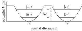
Figure S4: Truncated double-harmonic potential for modeling a single SCQ coupling to the cavity. In the limit of infinitely separated potential wells we approximate the system’s eigenstates with the two lowest bound states of isolated harmonic oscillators $\ket{0_{i}}$ and $\ket{1_{i}}$ ($i=\alpha,\beta$). The hybridization $\braket{1_{\alpha},0_{\beta}}{0_{\alpha},1_{\beta}}$ constitutes an approximation to the ring-to-center hopping $s(a)$ as a function of the spatial distance $a=x_{\beta}-x_{\alpha}$ of the potential wells.

While there are many sources for experimental losses, in our case a relevant quantity is the noise introduced by imperfections of the displacement of the SCQs from the cavity. In order to estimate the magnitude of the resulting perturbations we consider a single realization of a SCQ coupled to a cavity, which can be described by a Jaynes-Cunnings model in the regime where only the two lowest-energy qubit states are relevant [43]. Assuming a small qubit-cavity detuning and that the effective qubit-cavity coupling is large, we can neglect states with more than one excitation in the cavity such that for the following estimate we assume a system of two harmonic oscillators truncated to the two lowest eigenstates as depicted in Fig. S4. For that model we can compute the hybridization between qubit and cavity in terms of the oscillator eigenstates, as a function of the spatial distance $a$. At resonance where the level-spacing in both oscillators is identical, $\omega_{\alpha}=\omega_{\beta}=\omega$, we can then deduce the ring-to-center hopping amplitude from the overlap between the ground state $\ket{0_{\alpha}}$ of one oscillator and the excited state $\ket{1_{\beta}}$ of the other oscillator

$$s(a)\approx\hbar\omega\braket{1_{\alpha},0_{\beta}}{0_{\alpha},1_{\beta}}=\hbar\omega\left(\frac{m_{e}\omega}{2\hbar}a^{2}-1\right)\mathrm{e}^{-\frac{m_{e}\omega}{4\hbar}a^{2}}\;.$$ (S18)

We can now introduce random variations $\delta a_{j}$ describing experimental imperfections of $a$ so that $a\rightarrow a+\delta a_{j}\equiv a_{j}$ for each qubit $j$ coupled to the cavity. We assume the $\delta a_{j}$ to be normal distributed, independent, random variables, $\delta a_{j}\sim\mathcal{N}(0,\Delta a^{2})$. Here, $\Delta a$ is fixed by the experimental precision. Evaluating the first moment of Eq. S18 with respect to the distribution of the $a_{j}$ yields an estimation for the ring-to-center hopping $s(a,\Delta a)=\langle\langle s\rangle\rangle_{a,\Delta a}$ while the second moment constitutes the standard deviation of the perturbations $\sigma^{2}(a,\Delta a)=\langle\langle s^{2}\rangle\rangle_{a,\Delta a}-\langle\langle s\rangle\rangle^{2}_{a,\Delta a}$.

The previous considerations enable us to numerically compute the optimal displacement $a_{\mathrm{opt}}$ of the SCQs from the cavity. We determined $a_{\mathrm{opt}}$ such that the ratio $r(a_{\mathrm{opt}},\Delta a)=s(a_{\mathrm{opt}},\Delta a)/\sigma(a_{\mathrm{opt}},\Delta a)$ is maximized, assuming precisions for positioning the qubits of $\Delta a\in[0.5\,\mathrm{nm},20\mathrm{nm}]$. In Fig. S5 $a_{\mathrm{opt}}$ is shown as a function of the precisions $\Delta a$ by the green curve, which is strictly increasing. The corresponding optimal ratio, shown by the purple curve, demonstrates that for practically feasible precisions $\Delta a\sim\mathcal{O}(1\,\mathrm{nm})$ large ratios $r(a_{\mathrm{opt}},\Delta a)\sim\mathcal{O}(10^{4})$ are in reach. We conclude that within the discussed approximations, the effect of model-imperfections in the ring-to-center hopping can be suppressed efficiently, if the SCQs are placed in the optimal distance $a_{\mathrm{opt}}$ from the cavity. In fact, for the optimal distance, the broadening of the characteristic clusters in the many-body spectrum of the unperturbed BHW, caused by experimental imperfections, is of the order $s\times 10^{-4}$.

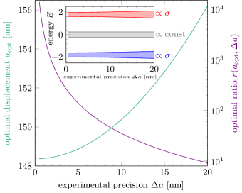
Figure S5: Numerically optimized mean distance $a_{\mathrm{opt}}$ and optimal ratio $r(a_{opt},\Delta a)$, depending on the experimental precision of the transmon qubit location $\Delta a$. The displayed data results from system sizes $L=20$ and $N=4$ particles, as well as a modulation of $k_{0}=\pi/2$. For readability reasons, the value of $s=0.4$ is kept constant with a typical transmon frequency of $\omega/2\pi=5\,\mathrm{GHz}$ and $s=12$. The inset plot shows the broadening of the separated many-particle clusters corresponding to an interval of three standard deviations, $E^{\mathrm{noise}}_{\mathrm{\pm}}\pm 3\sqrt{c_{\pm}}\sigma$.

VIII Solution strategy of the Bose-Hubbard wheel with control qubit

(a)

(b)

Figure S6: Energy differences between specific points in the two lowest clusters (i.e., $\nu=0$ and $\nu=1$) of the many-body spectrum for different $s$ and $s^{\prime}$ for $L=6,N=3$. In LABEL:sub@fig:gap:E1E2 we plot $\Delta E=\min\limits_{\mu}E_{0\mu}(N+1,N_{k_{0}}=2)-\max\limits_{\mu}E_{0\mu}(N,N_{k_{0}}=1)$, i.e., the separation between the lower edge of the $N_{k_{0}}=2$ and the upper edge of the $N_{k_{0}}=1$ cluster. This energy differences characterizes the gap in the effective, logical two-level system. LABEL:sub@fig:gap:EcE2 shows $\Delta E_{AH}=\min\left(\min\limits_{\mu,N_{k_{0}}=0,3}E_{0\mu}(N+1,N_{k_{0}}),\min\limits_{\mu,N_{k_{0}}=1,2}E_{1\mu}(N+1,N_{k_{0}})\right)-\max_{\mu,N_{k_{0}}=1,2}E_{0\mu}(N,N_{k_{0}})$, i.e., the separation between the lower edge of the central many-body eigenstate cluster and the upper edge of the lower many-body eigenstate cluster. This energy differences characterizes the separation of the effective, logical two-level system from the remaining many-body eigenstates, which can be compared to the anharmonicity of the constituting SCQ.

Let us now derive the matrix representation of the extended system, in which a newly introduced control qubit, denoted by $c$, couples to the center site of the wheel with amplitude $s^{\prime}$. The Hamiltonian of interest is given by

$$\hat{H}_{\mathrm{qubit}}=\hat{H}_{\mathrm{wheel}}+\hat{H}_{c}=-t\sum_{j=0}^{L-1}\left(\hat{h}^{\dagger}_{j}\hat{h}^{\phantom{\dagger}}_{j+1}+\mathrm{h.c.}\right)-\sum_{j=0}^{L-1}\left(s_{j}\hat{h}^{\dagger}_{j}\hat{h}^{\phantom{\dagger}}_{\odot}+\mathrm{h.c.}\right)+s^{\prime}(\hat{h}^{\dagger}_{\odot}\hat{h}^{\phantom{\dagger}}_{c}+\mathrm{h.c.})+\mu_{c}\hat{n}_{c}\;.$$ (S19)

Here, $\hat{h}^{(\dagger)}_{c}$ denotes the annihilation (creation) of a HCB on the control qubit. We introduce $\hat{N}_{k_{0}}=\hat{n}_{c}+\hat{n}_{k_{0}}$, the combined occupation of the $k_{0}$ mode, introduced in the section above, and the occupation of the control qubit. Since $\left[\hat{H},\hat{N}_{k_{0}}\right]=0$, the Hamiltonian can be block-diagonalized in $N_{k_{0}}$, $\braket{\mathrm{FS}_{N}}{\hat{H}_{\mathrm{qubit}}}{\mathrm{FS}_{N}}=\bigoplus_{N_{k_{0}}}\hat{h}(\mathrm{FS}_{N},N_{k_{0}})$. After re-sorting the blocks and grouping together those with the same total number of occupied modes in the Slater determinants and the $N_{k_{0}}$ sector, we obtain a $8\times 8$ matrix for a given $N$ made up of blocks for each $N_{k_{0}}$ with $N-N_{k_{0}}$ occupied modes in the Slater determinants, see Fig. S1 (right). Hence, we work in the basis

$$\ket{n_{c}}\ket{n_{k_{0}}}\ket{FS_{N-N_{k_{0}}}}\;,$$ (S20)

with possible values $n_{c}=0,1$ and $n_{k_{0}}=0,\pm$ (denoting the $n_{k_{0}}=1$ eigenstates), $2$, where the remaining eigenvalue problem of Eq. S19 can be solved in each block, individually. The matrix elements of each block are obtained in the following by letting Eq. S19 act on the states Eq. S20. For the $N_{k_{0}}=0,3$ sectors, the matrix elements are given by $E_{0}(FS_{N})$ and $E_{0}(FS_{N-3})$ respectively. For the $N_{k_{0}}=1$ sectors we have

$$\hat{H}_{c}\ket{n_{c}=0}\ket{\pm}\ket{FS_{N-1}}$$

$$=s^{\prime}\left(\hat{h}^{\dagger}_{c}\hat{h}^{\phantom{\dagger}}_{\odot}+\hat{h}^{\dagger}_{\odot}\hat{h}^{\phantom{\dagger}}_{c}\right)\ket{n_{c}=0}\left(d^{\pm}_{0}\ket{n_{k_{0},O}=1}\ket{n_{\odot}=0}+d^{\pm}_{1}\ket{n_{k_{0},O}=0}\ket{n_{\odot}=1}\right)\ket{FS_{N-1}}$$

$$=s^{\prime}d^{\pm}_{1}\ket{n_{c}=1}\ket{n_{k_{0},O}=0}\ket{n_{\odot}=0}\ket{FS_{N-1}}=s^{\prime}d^{\pm}_{1}\ket{n_{c}=1}\ket{0}\ket{FS_{N-1}}\;.$$

It follows that

$$\bra{FS_{N-1}}\bra{0}\bra{n_{c}=1}\hat{H}_{c}\ket{n_{c}=0}\ket{\pm}\ket{FS_{N-1}}=s^{\prime}d^{\pm}_{1}\;.$$ (S21)

All other matrix elements can be computed in a similar manner. Note that $\hat{H}_{\mathrm{wheel}}$ only has diagonal terms. Due to the orthogonality of the projected wheel eigenstates all other matrix elements vanish. $\hat{H}_{c}$ does not contribute diagonal terms as it changes the particle number on the control qubit and hence only connects states with different $n_{c}$. The entire $N_{k_{0}}=1$ subspace in matrix representation is given by

$$\hat{h}(\mathrm{FS}_{N-1},N_{k_{0}}=1)=\begin{pmatrix}E_{0}(\mathbf{k}_{N-1})+\mu_{c}&s^{\prime}(d^{+}_{1})&s^{\prime}(d^{-}_{1})\\ s^{\prime}(d^{+}_{1})^{*}&E_{1_{+}}(\mathbf{k}_{N-1})&0\\ s^{\prime}(d^{-}_{1})^{*}&0&E_{1_{-}}(\mathbf{k}_{N-1})\end{pmatrix}\;.$$ (S22)

For the $N_{k_{0}}=2$ sectors we have

$$\hat{H}_{c}\ket{n_{c}=1}\ket{\pm}\ket{FS_{N-2}}$$

$$=s^{\prime}\left(\hat{h}^{\dagger}_{c}\hat{h}^{\phantom{\dagger}}_{\odot}+\hat{h}^{\dagger}_{\odot}\hat{h}^{\phantom{\dagger}}_{c}\right)\ket{n_{c}=1}\left(d^{\pm}_{0}\ket{n_{k_{0},O}=1}\ket{n_{\odot}=0}+d^{\pm}_{1}\ket{n_{k_{0},O}=0}\ket{n_{\odot}=1}\right)\ket{FS_{N-2}}$$

$$=s^{\prime}d^{\pm}_{0}\ket{n_{c}=0}\ket{n_{k_{0},O}=1}\ket{n_{\odot}=1}\ket{FS_{N-2}}=s^{\prime}d^{\pm}_{0}\ket{n_{c}=0}\ket{2}\ket{FS_{N-2}}\;,$$

from which follows

$$\bra{FS_{N-2}}\bra{2}\bra{n_{c}=0}\hat{H}_{c}\ket{n_{c}=1}\ket{\pm}\ket{FS_{N-2}}=s^{\prime}d^{\pm}_{0}\;.$$ (S23)

The entire $N_{k_{0}}=2$ subspace in matrix representation is given by

$$\hat{h}(\mathrm{FS}_{N-2},N_{k_{0}}=2)=\begin{pmatrix}E_{1_{-}}(\mathbf{k}_{N-2})+\mu_{c}&0&s^{\prime}(d^{-}_{0})^{*}\\ 0&E_{1_{+}}(\mathbf{k}_{N-2})+\mu_{c}&s^{\prime}(d^{+}_{0})^{*}\\ s^{\prime}d^{-}_{0}&s^{\prime}d^{+}_{0}&E_{2}(\mathbf{k}_{N-2})\end{pmatrix}\;.$$ (S24)

These results are then used for numerical diagonalization. Arbitrary states from the respective sectors $N_{k_{0}}$ in a system of $N$ particles are denoted as follows

$$\ket{E_{\mu}(N,N_{k_{0}}=0)}=\ket{\varnothing}\ket{FS_{N}}_{\mu}$$ (S25)

$$\ket{E_{\nu\mu}(N,N_{k_{0}}=1)}=\left[v^{\nu\mu}_{0}\ket{1,0}+v^{\nu\mu}_{+}\ket{0,+}+v^{\nu\mu}_{-}\ket{0,-}\right]\ket{FS_{N-1}}_{\mu}$$ (S26)

$$\ket{E_{\nu\mu}(N,N_{k_{0}}=2)}=\left[w^{\nu\mu}_{-}\ket{1,-}+w^{\nu\mu}_{+}\ket{1,+}+w^{\nu\mu}_{2}\ket{0,2}\right]\ket{FS_{N-2}}_{\mu}$$ (S27)

$$\ket{E_{\mu}(N,N_{k_{0}}=3)}=\ket{1,2}\ket{FS_{N-3}}_{\mu}$$ (S28)

where $\mu\in\binom{L-1}{N-N_{k_{0}}}$ enumerates the Slater determinant outside of the $N_{k_{0}}$ subspace (for simplicity, this index has been dropped in the main text and the states are written as $\ket{E_{\nu}(N,N_{k_{0}})}=\ket{\nu_{N_{k_{0}}}}\otimes\ket{\mathrm{FS}_{N-N_{k_{0}}}}$ with $\nu_{N_{k_{0}}}=0,\dots,d_{N_{k_{0}}}-1$ where $d_{N_{k_{0}}}$ denotes the dimension of each $N_{k_{0}}$ block) and we use the abbreviation $\ket{n_{c},n_{k_{0}}}$. For the non-trivial $N_{k_{0}}=1,2$ sectors, there is an additional index $\nu$ denoting all three eigenstates for a given $\mu$. Note that each of the corresponding energies can be directly identified with one of the three branches in the spectrum and $\nu=0$ corresponds to the low-lying BEC sector which is of particular interest.

Given the many-body energies, we can characterize the typical energy scales relevant for the logical qubit setup. First, there is the energy gap between the two logical qubit states

$$\Delta E=\min\limits_{\mu}E_{0\mu}(N+1,N_{k_{0}}=2)-\max\limits_{\mu}E_{0\mu}(N,N_{k_{0}}=1)\;,$$ (S29)

which we show exemplary in Fig. S6a for a fixed system size and particle number, varying the couplings $s,s^{\prime}$. The second relevant energy scale is the separation of the two logical qubit states from the remaining part of the many-body spectrum

$$\Delta E_{AH}=\min\left(\min\limits_{\mu,N_{k_{0}}=0,3}E_{0\mu}(N+1,N_{k_{0}}),\min\limits_{\mu,N_{k_{0}}=1,2}E_{1\mu}(N+1,N_{k_{0}})\right)-\max_{\mu,N_{k_{0}}=1,2}E_{0\mu}(N,N_{k_{0}})\;.$$ (S30)

This quantity is shown in Fig. S6b using the same parameters as before.

The structure of the eigenstates of the reduced Hamiltonians $\hat{h}(\mathrm{FS}_{N-N_{k_{0}}},N_{k_{0}})$, as well as the occupation of the control qubit can also be understood by considering the control qubit as perturbation in $s^{\prime}/\tilde{s}$. Expanding $\hat{h}(\mathrm{FS}_{N-N_{k_{0}}},N_{k_{0}})$ in the tensor product basis of eigenstates of the reduced wheel $\ket{E_{n_{k_{0}}}(\mathrm{FS}_{N-n_{k_{0}}})}$ and the control qubit $\ket{n_{c}}$, one readily finds that the first non-trivial correction appears in second order $s^{\prime}/\tilde{s}$. In the following we will temporarily drop the Slater determinants $\mu$. The correction to the odd parity $N_{k_{0}}=1$ eigenstate is given by

$$\ket{E_{1}(N,N_{k_{0}}=1)} =\ket{1,0}+\mathcal{O}\left(\frac{s^{\prime}}{\tilde{s}}\right)\sum_{n_{k_{0}}=\pm}\ket{0,n_{k_{0}}}\;.$$ (S31)

For the even parity eigenstates with $\nu=0,2$ one equivalently finds

$$\ket{E_{\nu}(N,N_{k_{0}}=1)} =\ket{0,\pm}+\mathcal{O}\left(\frac{s^{\prime}}{\tilde{s}}\right)\ket{0,0}\;.$$ (S32)

Therefore, the probe-site occupations in the eigenstates of the $N_{k_{0}}=1$ sector exhibit second-order corrections in $s^{\prime}/\tilde{s}$:

$$\bra{E_{1}(N,N_{k_{0}}=1)}\hat{n}_{c}\ket{E_{1}(N,N_{k_{0}}=1)} =1-\mathcal{O}\left(\left(\frac{s^{\prime}}{\tilde{s}}\right)^{2}\right)\;,$$ (S33)

$$\bra{E_{\nu}(N,N_{k_{0}}=1)}\hat{n}_{c}\ket{E_{\nu}(N,N_{k_{0}}=1)} =\mathcal{O}\left(\left(\frac{s^{\prime}}{\tilde{s}}\right)^{2}\right),$$ (S34)

Similarly, for the $N_{k_{0}}=2$ sector the probe-site occupations evaluate to

$$\bra{E_{1}(N,N_{k_{0}}=2)}\hat{n}_{c}\ket{E_{1}(N,N_{k_{0}}=2)} =\mathcal{O}\left(\left(\frac{s^{\prime}}{\tilde{s}}\right)^{2}\right)\;,$$ (S35)

$$\bra{E_{\nu}(N,N_{k_{0}}=2)}\hat{n}_{c}\ket{E_{\nu}(N,N_{k_{0}}=2)} =1-\mathcal{O}\left(\left(\frac{s^{\prime}}{\tilde{s}}\right)^{2}\right)\;,$$ (S36)

IX Fidelity of $X$-gate application

In the following, we will consider systems at half filling $N=L/2$. For later convenience and using Eq. S28 we compute

$$\hat{c}^{\dagger}_{c}\ket{E_{\mu}(N,N_{k_{0}}=0)}=\ket{n_{c}=1}\ket{FS_{N}}_{\mu}$$

$$\hat{c}^{\dagger}_{c}\ket{E_{\nu\mu}N,N_{k_{0}}=1}=\left[v^{\nu\mu}_{+}\ket{n_{c}=1,+}+v^{\nu\mu}_{-}\ket{n_{c}=1,-}\right]\ket{FS_{N-1}}_{\mu}$$

$$\hat{c}^{\dagger}_{c}\ket{E_{\nu\mu}(N,N_{k_{0}}=2)}=w^{\nu\mu}_{2}\ket{n_{c}=1,2}\ket{FS_{N-2}}_{\mu}$$

$$\hat{c}^{\dagger}_{c}\ket{E_{\mu}(N,N_{k_{0}}=3)}=0$$

We define the $X$-gate fidelity at zero temperature as the probability to create a state in the lower branch of the $N_{k_{0}}=2$ sector of a system realization with $N+1$ particles by exciting a state in the lower branch of the $N_{k_{0}}=1$ sector of a system with $N$ particles,

$$F\equiv\absolutevalue{\bra{E_{0\mu}(N+1,N_{k_{0}}=2)}\hat{c}^{\dagger}_{c}\ket{E_{0\mu}(N,N_{k_{0}}=1)}}^{2}=\absolutevalue{(\tilde{w}^{0\mu}_{+})^{*}v^{0\mu}_{+}+(\tilde{w}^{0\mu}_{-})^{*}v^{0\mu}_{-}}^{2}\;.$$ (S37)

The tilde highlights the fact that we are looking at two different initializations of the wheel-probe system with $N$ and $(N+1)$ particles denoted by coefficients without and with tilde. For the finite temperature treatment we introduce the thermal density operator of the system

$$\hat{\rho}(T,N)=\frac{1}{Z}\sum_{i}e^{-\beta E_{i}^{N}}\ket{\Psi_{i}(N)}\bra{\Psi_{i}(N)}=\frac{1}{Z}\sum_{N_{k_{0}}=0}^{3}\sum_{\mu}^{\binom{L-1}{N-N_{k_{0}}}}\sum_{\nu}^{d_{N_{k_{0}}}}e^{-\beta E_{\nu,\mu}^{N}(N_{k_{0}})}\ket{E_{\nu\mu}(N,N_{k_{0}})}\bra{E_{\nu\mu}(N,N_{k_{0}})}$$ (S38)

with $\beta=1/k_{B}T$, $d(N_{k_{0}})$ denotes the dimension of the $N_{k_{0}}$ subspace (we will drop the index $\nu$ in the case $d(N_{k_{0}})=1$) and the partition function

$$Z=\sum_{N_{k_{0}}=0}^{3}\sum_{\mu}^{\binom{L-1}{N-N_{k_{0}}}}\sum_{\nu}^{d_{N_{k_{0}}}}e^{-\beta E_{\nu\mu}^{N}(N_{k_{0}})}\;.$$ (S39)

The energies are normalized to the ground state energy. To examine the effect of an excitation on the control qubit we consider the density operator

$$\hat{\rho}_{1}(T)=\hat{c}^{\dagger}_{c}\hat{\rho}(T)\hat{c}^{\phantom{\dagger}}_{c}=\frac{1}{Z}\sum_{\mu}^{\binom{L-1}{N}}e^{-\beta E^{N}_{\mu}(0)}\ket{n_{c}=1}\ket{FS_{N}}_{\mu}\bra{n_{c}=1}\bra{FS_{N}}_{\mu}$$

$$+\sum_{\mu}^{\binom{L-1}{N-1}}\sum_{\nu}^{d_{1}}e^{-\beta E^{N}_{\nu\mu}(1)}\left[v^{\nu\mu}_{+}\ket{n_{c}=1,+}+v^{\nu\mu}_{-}\ket{n_{c}=1,-}\right]\ket{FS_{N-1}}_{\mu}\left[(v^{\nu\mu}_{+})^{*}\bra{n_{c}=1,+}+(v^{\nu\mu}_{-})^{*}\bra{n_{c}=1,-}\right]\bra{FS_{N-1}}_{\mu}$$

$$+\sum_{\mu}^{\binom{L-1}{N-2}}\sum_{\nu}^{d_{2}}e^{-\beta E^{N}_{\nu\mu}(2)}\absolutevalue{w^{\nu\mu}_{2}}^{2}\ket{n_{c}=1,2}\ket{FS_{N-2}}_{\mu}\bra{n_{c}=1,2}\bra{FS_{N-2}}_{\mu}]\;.$$ (S40)

The fidelity $F(T)$ is then computed as the probability to find any state $\ket{E_{0\mu}(N+1,N_{k_{0}}=2)}$ in the low-lying BEC sector of the wheel-control qubit system filled with $N+1$ particles after the excitation. After some algebra using the orthogonality of Slater determinants we arrive at

$$F(T) \equiv\sum_{\mu}^{\binom{L-1}{N-1}}\bra{E_{0\mu}(N+1,N_{k_{0}}=2)}\hat{c}^{\dagger}_{c}\hat{\rho}(T)\hat{c}^{\phantom{\dagger}}_{c}\ket{E_{0\mu}(N+1,N_{k_{0}}=2)}$$

$$=\frac{1}{Z}\sum_{\mu}^{\binom{L-1}{N-1}}\sum^{d_{1}}_{\nu}e^{-\beta E^{N}_{\nu\mu}(1)}\absolutevalue{\left[(\tilde{w}^{0\mu}_{-})^{*}\bra{n_{c}=1,-}+(\tilde{w}^{0\mu}_{+})^{*}\bra{n_{c}=1,+}+(w^{0\mu}_{2})^{*}\bra{n_{c}=0,2}\right]\left[v^{\nu\mu}_{+}\ket{n_{c}=1,+}+v^{\nu\mu}_{-}\ket{n_{c}=1,-}\right]}^{2}$$

$$=\frac{1}{Z}\sum_{\mu}^{\binom{L-1}{N-1}}\sum^{d_{1}}_{\nu}e^{-\beta E^{N}_{\nu\mu}(1)}\absolutevalue{(\tilde{w}^{0\mu}_{+})^{*}v^{\nu\mu}_{+}+(\tilde{w}^{0\mu}_{-})^{*}v^{\nu\mu}_{-}}^{2}\;.$$ (S41)

Only the contributions from the $N_{k_{0}}=1$ sector are relevant since the Slater determinants have to coincide with those of $\ket{E_{0\mu}(N+1,N_{k_{0}}=2)}$, which cannot happen in any other sector, because they have a different number of modes in their Slater determinants.

X Sampling Scheme

The system is prepared in a state described by Eq. S38 and a measurement of the control qubit occupation is performed after exciting the control qubit, i.e. we compute the probability to find the system in the states $\ket{n_{c}=1}\ket{FS_{N}}_{\mu},\ket{n_{c}=1,+}\ket{FS_{N-1}}_{\mu},\ket{n_{c}=1,-}\ket{FS_{N-1}}_{\mu},\ket{n_{c}=1,2}\ket{FS_{N-2}}_{\mu}$ after the excitation.

$$\bra{n_{c}=1}\hat{\rho}_{1}(T)\ket{n_{c}=1}$$

$$=\sum_{\mu}\bra{n_{c}=1}\bra{FS_{N}}_{\mu}\hat{\rho}_{1}(T)\ket{n_{c}=1}\ket{FS_{N}}_{\mu}+\sum_{\mu}\bra{n_{c}=1,+}\bra{FS_{N-1}}_{\mu}\hat{\rho}_{1}(T)\ket{n_{c}=1,+}\ket{FS_{N-1}}_{\mu}+$$

$$\sum_{\mu}\bra{n_{c}=1,-}\bra{FS_{N-1}}_{\mu}\hat{\rho}_{1}(T)\ket{n_{c}=1,-}\ket{FS_{N-1}}_{\mu}+\sum_{\mu}\bra{n_{c}=1,2}\bra{FS_{N-2}}_{\mu}\hat{\rho}_{1}(T)\ket{n_{c}=1,2}\ket{FS_{N-2}}_{\mu}$$

$$=\frac{1}{Z}\left[\sum^{\binom{L-1}{N}}_{\mu}e^{-\beta E^{N}_{\mu}(0)}+\sum^{\binom{L-1}{N-1}}_{\mu}\sum_{\nu}^{d_{1}}e^{-\beta E^{N}_{\nu\mu}(1)}\left[\absolutevalue{v_{+}^{\nu\mu}}^{2}+\absolutevalue{v_{-}^{\nu\mu}}^{2}\right]+\sum^{\binom{L-1}{N-2}}_{\mu}\sum_{\nu}^{d_{2}}e^{-\beta E^{N}_{\nu\mu}(2)}\absolutevalue{w_{2}^{\nu\mu}}^{2}\right]$$ (S42)

References

- Grover [1996] L. K. Grover, A fast quantum mechanical algorithm for database search (1996), arXiv:quant-ph/9605043 [quant-ph] .
- Shor [1999] P. W. Shor, Polynomial-time algorithms for prime factorization and discrete logarithms on a quantum computer, SIAM Review 41, 303 (1999), https://doi.org/10.1137/S0036144598347011 .
- Preskill [2018] J. Preskill, Quantum Computing in the NISQ era and beyond, Quantum 2, 79 (2018).
- Unruh [1995] W. G. Unruh, Maintaining coherence in quantum computers, Phys. Rev. A 51, 992 (1995).
- Knill et al. [1998] E. Knill, R. Laflamme, and W. H. Zurek, Resilient quantum computation, Science 279, 342 (1998), https://www.science.org/doi/pdf/10.1126/science.279.5349.342 .
- Preskill [1998] J. Preskill, Fault-tolerant quantum computation, in Introduction to Quantum Computation and Information (1998) pp. 213–269.
- Aharonov and Ben-Or [2008] D. Aharonov and M. Ben-Or, Fault-tolerant quantum computation with constant error rate, SIAM Journal on Computing 38, 1207 (2008), https://doi.org/10.1137/S0097539799359385 .
- Li and Benjamin [2017] Y. Li and S. C. Benjamin, Efficient variational quantum simulator incorporating active error minimization, Phys. Rev. X 7, 021050 (2017).
- Temme et al. [2017] K. Temme, S. Bravyi, and J. M. Gambetta, Error mitigation for short-depth quantum circuits, Phys. Rev. Lett. 119, 180509 (2017).
- Cai et al. [2023] Z. Cai, R. Babbush, S. C. Benjamin, S. Endo, W. J. Huggins, Y. Li, J. R. McClean, and T. E. O’Brien, Quantum error mitigation, Rev. Mod. Phys. 95, 045005 (2023).
- Calderbank and Shor [1996] A. R. Calderbank and P. W. Shor, Good quantum error-correcting codes exist, Phys. Rev. A 54, 1098 (1996).
- Steane [1996] A. Steane, Multiple-particle interference and quantum error correction, Proceedings of the Royal Society A 452, 10.1098/rspa.1996.0136 (1996).
- Dennis et al. [2002] E. Dennis, A. Kitaev, A. Landahl, and J. Preskill, Topological quantum memory, J. Math. Phys. 43, 4452– (2002).
- Gottesman [2010] D. Gottesman, An introduction to quantum error correction and fault-tolerant quantum computation, Proceedings of Symposia in Applied Mathematics 68, 10.1090/psapm/068 (2010).
- Kitaev [1997] A. Y. Kitaev, Quantum computations: algorithms and error correction, Russian Mathematical Surveys 52, 1191 (1997).
- Kitaev [2003] A. Kitaev, Fault-tolerant quantum computation by anyons, Annals of Physics 303, 2 (2003).
- Kim et al. [2023] Y. Kim, A. Eddins, S. Anand, K. X. Wei, E. van den Berg, S. Rosenblatt, H. Nayfeh, Y. Wu, M. Zaletel, K. Temme, and A. Kandala, Evidence for the utility of quantum computing before fault tolerance, Nature 618, 500 (2023).
- Tindall et al. [2024] J. Tindall, M. Fishman, E. M. Stoudenmire, and D. Sels, Efficient tensor network simulation of ibm’s eagle kicked ising experiment, PRX Quantum 5, 010308 (2024).
- Cai [2021] Z. Cai, Multi-exponential error extrapolation and combining error mitigation techniques for nisq applications, npj Quantum Information 7, 80 (2021).
- Krinner et al. [2022] S. Krinner, N. Lacroix, A. Remm, A. Di Paolo, E. Genois, C. Leroux, C. Hellings, S. Lazar, F. Swiadek, J. Herrmann, G. J. Norris, C. K. Andersen, M. Müller, A. Blais, C. Eichler, and A. Wallraff, Realizing repeated quantum error correction in a distance-three surface code, Nature 605, 10.1038/s41586-022-04566-8 (2022).
- Takeda et al. [2022] K. Takeda, A. Noiri, T. Nakajima, T. Kobayashi, and S. Tarucha, Quantum error correction with silicon spin qubits, Nature 608, 682 (2022).
- Ryan-Anderson et al. [2022] C. Ryan-Anderson, N. C. Brown, M. S. Allman, B. Arkin, G. Asa-Attuah, C. Baldwin, J. Berg, J. G. Bohnet, S. Braxton, N. Burdick, J. P. Campora, A. Chernoguzov, J. Esposito, B. Evans, D. Francois, J. P. Gaebler, T. M. Gatterman, J. Gerber, K. Gilmore, D. Gresh, A. Hall, A. Hankin, J. Hostetter, D. Lucchetti, K. Mayer, J. Myers, B. Neyenhuis, J. Santiago, J. Sedlacek, T. Skripka, A. Slattery, R. P. Stutz, J. Tait, R. Tobey, G. Vittorini, J. Walker, and D. Hayes, Implementing fault-tolerant entangling gates on the five-qubit code and the color code (2022), arXiv:2208.01863 [quant-ph] .
- Acharya et al. [2023] R. Acharya, I. Aleiner, R. Allen, T. I. Andersen, M. Ansmann, F. Arute, K. Arya, A. Asfaw, J. Atalaya, R. Babbush, D. Bacon, J. C. Bardin, J. Basso, A. Bengtsson, S. Boixo, G. Bortoli, A. Bourassa, J. Bovaird, L. Brill, M. Broughton, B. B. Buckley, D. A. Buell, T. Burger, B. Burkett, N. Bushnell, Y. Chen, Z. Chen, B. Chiaro, J. Cogan, R. Collins, P. Conner, W. Courtney, A. L. Crook, B. Curtin, D. M. Debroy, A. Del Toro Barba, S. Demura, A. Dunsworth, D. Eppens, C. Erickson, L. Faoro, E. Farhi, R. Fatemi, L. Flores Burgos, E. Forati, A. G. Fowler, B. Foxen, W. Giang, C. Gidney, D. Gilboa, M. Giustina, A. Grajales Dau, J. A. Gross, S. Habegger, M. C. Hamilton, M. P. Harrigan, S. D. Harrington, O. Higgott, J. Hilton, M. Hoffmann, S. Hong, T. Huang, A. Huff, W. J. Huggins, L. B. Ioffe, S. V. Isakov, J. Iveland, E. Jeffrey, Z. Jiang, C. Jones, P. Juhas, D. Kafri, K. Kechedzhi, J. Kelly, T. Khattar, M. Khezri, M. Kieferová, S. Kim, A. Kitaev, P. V. Klimov, A. R. Klots, A. N. Korotkov, F. Kostritsa, J. M. Kreikebaum, D. Landhuis, P. Laptev, K.-M. Lau, L. Laws, J. Lee, K. Lee, B. J. Lester, A. Lill, W. Liu, A. Locharla, E. Lucero, F. D. Malone, J. Marshall, O. Martin, J. R. McClean, T. McCourt, M. McEwen, A. Megrant, B. Meurer Costa, X. Mi, K. C. Miao, M. Mohseni, S. Montazeri, A. Morvan, E. Mount, W. Mruczkiewicz, O. Naaman, M. Neeley, C. Neill, A. Nersisyan, H. Neven, M. Newman, J. H. Ng, A. Nguyen, M. Nguyen, M. Y. Niu, T. E. O’Brien, A. Opremcak, J. Platt, A. Petukhov, R. Potter, L. P. Pryadko, C. Quintana, P. Roushan, N. C. Rubin, N. Saei, D. Sank, K. Sankaragomathi, K. J. Satzinger, H. F. Schurkus, C. Schuster, M. J. Shearn, A. Shorter, V. Shvarts, J. Skruzny, V. Smelyanskiy, W. C. Smith, G. Sterling, D. Strain, M. Szalay, A. Torres, G. Vidal, B. Villalonga, C. Vollgraff Heidweiller, T. White, C. Xing, Z. J. Yao, P. Yeh, J. Yoo, G. Young, A. Zalcman, Y. Zhang, N. Zhu, and G. Q. AI, Suppressing quantum errors by scaling a surface code logical qubit, Nature 614, 676 (2023).
- Bluvstein et al. [2024] D. Bluvstein, S. J. Evered, A. A. Geim, S. H. Li, H. Zhou, T. Manovitz, S. Ebadi, M. Cain, M. Kalinowski, D. Hangleiter, J. P. Bonilla Ataides, N. Maskara, I. Cong, X. Gao, P. Sales Rodriguez, T. Karolyshyn, G. Semeghini, M. J. Gullans, M. Greiner, V. Vuletić, and M. D. Lukin, Logical quantum processor based on reconfigurable atom arrays, Nature 626, 58 (2024).
- Krantz et al. [2019] P. Krantz, M. Kjaergaard, F. Yan, T. P. Orlando, S. Gustavsson, and W. D. Oliver, A quantum engineer’s guide to superconducting qubits, Applied Physics Reviews 6, 021318 (2019), https://pubs.aip.org/aip/apr/article-pdf/doi/10.1063/1.5089550/16667201/021318_1_online.pdf .
- IBM [2023] IBM, The hardware and software for the era of quantum utility is here (2023).
- DiVincenzo [2009] D. P. DiVincenzo, Fault-tolerant architectures for superconducting qubits, Physica Scripta 2009, 014020 (2009).
- Gambetta et al. [2017] J. M. Gambetta, J. M. Chow, and M. Steffen, Building logical qubits in a superconducting quantum computing system, npj Quantum Information 3, 2 (2017).
- Andersen et al. [2023] T. I. Andersen, Y. D. Lensky, K. Kechedzhi, I. K. Drozdov, A. Bengtsson, S. Hong, A. Morvan, X. Mi, A. Opremcak, R. Acharya, R. Allen, M. Ansmann, F. Arute, K. Arya, A. Asfaw, J. Atalaya, R. Babbush, D. Bacon, J. C. Bardin, G. Bortoli, A. Bourassa, J. Bovaird, L. Brill, M. Broughton, B. B. Buckley, D. A. Buell, T. Burger, B. Burkett, N. Bushnell, Z. Chen, B. Chiaro, D. Chik, C. Chou, J. Cogan, R. Collins, P. Conner, W. Courtney, A. L. Crook, B. Curtin, D. M. Debroy, A. Del Toro Barba, S. Demura, A. Dunsworth, D. Eppens, C. Erickson, L. Faoro, E. Farhi, R. Fatemi, V. S. Ferreira, L. F. Burgos, E. Forati, A. G. Fowler, B. Foxen, W. Giang, C. Gidney, D. Gilboa, M. Giustina, R. Gosula, A. G. Dau, J. A. Gross, S. Habegger, M. C. Hamilton, M. Hansen, M. P. Harrigan, S. D. Harrington, P. Heu, J. Hilton, M. R. Hoffmann, T. Huang, A. Huff, W. J. Huggins, L. B. Ioffe, S. V. Isakov, J. Iveland, E. Jeffrey, Z. Jiang, C. Jones, P. Juhas, D. Kafri, T. Khattar, M. Khezri, M. Kieferová, S. Kim, A. Kitaev, P. V. Klimov, A. R. Klots, A. N. Korotkov, F. Kostritsa, J. M. Kreikebaum, D. Landhuis, P. Laptev, K. M. Lau, L. Laws, J. Lee, K. W. Lee, B. J. Lester, A. T. Lill, W. Liu, A. Locharla, E. Lucero, F. D. Malone, O. Martin, J. R. McClean, T. McCourt, M. McEwen, K. C. Miao, A. Mieszala, M. Mohseni, S. Montazeri, E. Mount, R. Movassagh, W. Mruczkiewicz, O. Naaman, M. Neeley, C. Neill, A. Nersisyan, M. Newman, J. H. Ng, A. Nguyen, M. Nguyen, M. Y. Niu, T. E. O’Brien, S. Omonije, A. Petukhov, R. Potter, L. P. Pryadko, C. Quintana, C. Rocque, N. C. Rubin, N. Saei, D. Sank, K. Sankaragomathi, K. J. Satzinger, H. F. Schurkus, C. Schuster, M. J. Shearn, A. Shorter, N. Shutty, V. Shvarts, J. Skruzny, W. C. Smith, R. Somma, G. Sterling, D. Strain, M. Szalay, A. Torres, G. Vidal, B. Villalonga, C. V. Heidweiller, T. White, B. W. K. Woo, C. Xing, Z. J. Yao, P. Yeh, J. Yoo, G. Young, A. Zalcman, Y. Zhang, N. Zhu, N. Zobrist, H. Neven, S. Boixo, A. Megrant, J. Kelly, Y. Chen, V. Smelyanskiy, E. A. Kim, I. Aleiner, P. Roushan, G. Q. AI, and Collaborators, Non-abelian braiding of graph vertices in a superconducting processor, Nature 618, 264 (2023).
- Blais et al. [2021a] A. Blais, A. L. Grimsmo, S. M. Girvin, and A. Wallraff, Circuit quantum electrodynamics, Rev. Mod. Phys. 93, 025005 (2021a).
- van Dongen et al. [1991] P. G. J. van Dongen, J. A. Vergés, and D. Vollhardt, The hubbard star, Zeitschrift für Physik B Condensed Matter 84, 383 (1991).
- Vidal et al. [2011] E. J. G. G. Vidal, R. P. A. Lima, and M. L. Lyra, Bose-einstein condensation in the infinitely ramified star and wheel graphs, Phys. Rev. E 83, 061137 (2011).
- Máté et al. [2021] M. Máté, Ö. Legeza, R. Schilling, M. Yousif, and C. Schilling, How creating one additional well can generate bose-einstein condensation, Communications Physics 4, 29 (2021).
- Wilke et al. [2023] R. H. Wilke, T. Köhler, F. A. Palm, and S. Paeckel, Symmetry-protected bose-einstein condensation of interacting hardcore bosons, Communications Physics 6, 182 (2023).
- Rigol and Muramatsu [2004] M. Rigol and A. Muramatsu, Emergence of quasicondensates of hard-core bosons at finite momentum, Phys. Rev. Lett. 93, 230404 (2004).
- Rigol and Muramatsu [2005] M. Rigol and A. Muramatsu, Ground-state properties of hard-core bosons confined on one-dimensional optical lattices, Phys. Rev. A 72, 013604 (2005).
- Lieb [1963] E. H. Lieb, Exact analysis of an interacting bose gas. ii. the excitation spectrum, Phys. Rev. 130, 1616 (1963).
- Lieb and Liniger [1963] E. H. Lieb and W. Liniger, Exact analysis of an interacting bose gas. i. the general solution and the ground state, Phys. Rev. 130, 1605 (1963).
- Tennie et al. [2017] F. Tennie, V. Vedral, and C. Schilling, Universal upper bounds on the bose-einstein condensate and the hubbard star, Phys. Rev. B 96, 064502 (2017).
- [40] S. S. Material, Link will be added.
- Yoshihara et al. [2017] F. Yoshihara, T. Fuse, S. Ashhab, K. Kakuyanagi, S. Saito, and K. Semba, Superconducting qubit–oscillator circuit beyond the ultrastrong-coupling regime, Nature Physics 13, 44 (2017).
- Roth et al. [2023] T. E. Roth, R. Ma, and W. C. Chew, The transmon qubit for electromagnetics engineers: An introduction, IEEE Antennas and Propagation Magazine 65, 8–20 (2023).
- Blais et al. [2021b] A. Blais, A. L. Grimsmo, S. Girvin, and A. Wallraff, Circuit quantum electrodynamics, Reviews of Modern Physics 93, 10.1103/revmodphys.93.025005 (2021b).