Wavelets for $L^{2}(B(0,1))$ using Zernike polynomials

Abstract.

A set of orthogonal polynomials on the unit disk $B(0,1)$ known as Zernike polynomials are commonly used in the analysis and evaluation of optical systems. Here Zernike polynomials are used to construct wavelets for polynomial subspaces of $L^{2}(B(0,1)).$ This naturally leads to a multiresolution analysis of $L^{2}(B(0,1)).$ Previously, other authors have dealt with the one dimensional case, and used orthogonal polynomials of a single variable to construct time localized bases for polynomial subspaces of an $L^{2}$-space with arbitrary weight. Due to the nature of Zernike polynomials, the wavelet construction given here is well-suited for the analysis of two-dimensional signals defined on circular domains. This is shown by some experimental results done on corneal data.

Keywords:

2000 MSC:

1. Introduction

1.1. Background

Wavelets can be viewed as a tool to obtain expansions of functions in Hilbert spaces. Traditionally, a wavelet system is made of a function $\psi$ and all integer translations and dilations of $\psi:$

$$\psi_{j,k}=2^{j/2}\psi(2^{j}x-k),\quad x\in\mathbb{R},\ j,k\in\mathbb{Z},$$

such that $\{\psi_{j,k}\}_{j,k\in\mathbb{Z}}$ is an orthonormal basis (ONB) of $L^{2}(\mathbb{R}).$ The first example of such a $\psi$ was given by Haar in 1910 [6], and is called the Haar wavelet. Multiresolution analysis (MRA) is a tool to construct wavelets, and is a central ingredient in wavelet analysis. The general framework of MRA was devised by Mallat [10] and Meyer [11]. An MRA consists of a nested sequence $\{V_{j}\}_{j\in\mathbb{Z}}$ of closed subspaces of $L^{2}(\mathbb{R}),$ giving a decomposition of $L^{2}(\mathbb{R}).$ In wavelet analysis, a signal $f$ is decomposed into pieces, each subspace $V_{j}$ has a piece of $f.$ These pieces, or projections, of $f$ give finer and finer details of $f.$ In connection with approximation theory, approximation of $f$ in $L^{2}(\mathbb{R})$ can be performed via the projection of $f$ on one of these subspaces.

When a signal $f$ is represented in terms of a wavelet basis $\{\psi_{j,k}\}_{j,k\in\mathbb{Z}}$, then it can be written as

(1.1) $$f(x)=\sum_{j,k}c_{j,k}\psi_{j,k}(x).$$

A representation such as (1.1) gives useful information about when or where a certain frequency occurs in the considered signal $f.$ Different frequencies appear with different values of $j$ and this fact is useful in time-frequency or space-frequency analysis. Slow oscillations of $f$ will lead to nonzero coefficients for small values of $j,$ whereas fast oscillations will lead to nonzero coefficients for large values of $j.$ The location of a frequency is indicated by the corresponding $k.$ Such information regarding the location of a frequency is not evident in the Fourier series or Fourier-Zernike series (see (1.6) below) of a signal.

A set of two dimensional orthogonal functions defined on the unit disk $B(0,1)$, called Zernike polynomials, is used in the analysis of optical systems by expanding optical wavefront functions as series of these functions [15, 12]. The Zernike polynomials form an orthonormal basis for $L^{2}(B(0,1)),$ the space of square integrable functions on the unit disc, and can thus be used to effectively represent signals on circular domains [15, 12]. In this work, Zernike polynomials have been used to construct wavelets for polynomial subspaces of $L^{2}(B(0,1)).$ This is inspired by previous work done in [4] for the 1D case where the authors have used orthogonal polynomials to construct time-localized bases for polynomial subspaces of an $L^{2}$-space with arbitrary weight. The construction in [4] is based on the general theory of kernel polynomials, and this has been used to get a multiresolution analysis (MRA) of a weighted $L^{2}$-space that is different from traditional MRA. Similarly, we will be able to get a multiresolution of $L^{2}(B(0,1))$ by using the wavelet spaces constructed out of the Zernike polynomials. In [8], a decomposition of the space $L^{2}(-1,1)$ has been investigated using wavelets from algebraic polynomials using Chebyshev-weight. Even though multidimensional wavelets have been constructed and studied by some researchers (see, for example, [9, 5]), such analysis is suited for rectangular domains, and the resulting wavelets are meant for functions on $\mathbb{R}^{d},$ $d\geq 2.$ The wavelet analysis that is proposed here using Zernike polynomials is suitable for signals on circular domains like that of optical data, and can be very useful in the analysis of such data. The primary motivation is efficient representation of 2D signals defined on circular domains, such as corneal surfaces and certain optical systems, by using wavelets constructed from Zernike polynomials. Good models of corneal surfaces are important for characterizing aberrations and detecting abnormalities of the cornea. We have implemented our 2D wavelets in the reconstruction of corneal data from its wavelets coefficients, and used the information of the wavelet coefficients to study location of spatial frequency in the data.

1.2. Preliminaries and Notation

Let $\mathbb{N}_{0}=\{0,1,2,3,\ldots\}=\mathbb{N}\cup\{0\}.$ The Zernike polynomials are defined in terms of complex exponentials as

(1.2) $$Z_{n}^{m}(r,\phi)=\gamma_{n}^{m}R_{n}^{|m|}(r)e^{im\phi},\quad 0\leq r\leq 1,\ 0\leq\phi<2\pi,$$

where $n\in\mathbb{N}_{0},$ $|m|\leq n,$ $n-m$ is even, $\gamma_{n}^{m}$ is the normalization constant given by

$$\gamma_{n}^{m}=\sqrt{\frac{n+1}{\pi}}\quad\forall m,$$

$R_{n}^{|m|}$ are the radial parts of the polynomials given by

(1.3) $$R_{n}^{|m|}(r)=\sum_{s=0}^{(n-|m|)/2}\frac{(-1)^{s}(n-s)!}{s!((n+|m|)/2-s)!((n-|m|)/2-s)!}r^{n-2s}$$

and will be referred to as radial polynomials. When a single index notation is needed, the conversion from $Z_{n}^{m}$ to $Z_{j},$ $j\in\mathbb{N}_{0},$ is made by the formula

(1.4) $$j=\frac{n(n+2)+m}{2}.$$

It is known that the Zernike polynomials given in (1.2) form a complete orthonormal set [12] for $L^{2}(B(0,1)),$ the space of square integrable functions on the unit disk $B(0,1)=\{(x,y)\in\mathbb{R}^{2}:x^{2}+y^{2}\leq 1\},$ with respect to the inner product

(1.5) $$\langle f,g\rangle:=\int_{0}^{1}\int_{0}^{2\pi}f(r,\phi)\overline{g(r,\phi)}\ r\ d\phi\ dr.$$

In polar form, the Zernike polynomials of (1.2) can be written as

$$G^{m}_{n}(r,\phi)=\left\{\begin{array}[]{cc}\gamma^{m}_{n}R^{|m|}_{n}(r)\cos(m\phi),&\textrm{if $m\geq 0,$}\\ \gamma^{m}_{n}R^{|m|}_{n}(r)\sin(|m|\phi),&\textrm{if $m<0,$}\end{array}\right.$$

where $n\geq 0,$ $|m|\leq n,$ $n-m$ is even, $\gamma^{m}_{n}$ are normalization constants given by

$$\gamma_{n}^{m}=\left\{\begin{array}[]{cc}\sqrt{\frac{n+1}{\pi}}&\textrm{if}\ m=0\\ \sqrt{\frac{2(n+1)}{\pi}}&\textrm{if}\ m\neq 0,\end{array}\right.$$

and $R_{n}^{|m|}$ are radial polynomials already given in (1.3). Each $G^{m}_{n}(r,\phi)$ is a polynomial in $x$, $y$ of degree $n$, and $\{G^{m}_{n}(r,\phi)\}_{\begin{subarray}{c}n=0,|m|\leq n\\ (n-m)\textrm{even}\end{subarray}}^{\infty}$ form a complete orthonormal set in $L^{2}(B(0,1))$ with respect to the same inner product given above in (1.5) . Any $f\in L^{2}(B(0,1))$ can be written in terms of $Z^{m}_{n}$s or $G^{m}_{n}$s as follows.

(1.6) $$f(\rho,\theta) = \sum_{n=0}^{\infty}\sum_{\begin{subarray}{c}m=0\\ (n-m)\textrm{even}\end{subarray}}^{n}\left[A_{nm}\cos m\theta+B_{nm}\sin m\theta\right]R^{m}_{n}(\rho)$$

$$= \sum_{n=0}^{\infty}\sum_{\begin{subarray}{c}m=-n\\ (n-m)\textrm{even}\end{subarray}}^{n}c_{nm}e^{im\theta}R^{|m|}_{n}(\rho).$$

The connection between the corresponding coefficients is given by the following. For all $n\in\mathbb{N}_{0},$ $(n-m)$ even, $m\leq n,$

$$c_{nm} = \frac{A_{nm}-iB_{nm}}{2},\quad m\in\mathbb{N}_{0},$$

$$c_{n(-m)} = \frac{A_{nm}+iB_{nm}}{2},\quad m\in\mathbb{N},$$

and for all $n,m\in\mathbb{N}_{0},$ $(n-m)$ even, $m\leq n,$

$$A_{nm} = c_{nm}+c_{n(-m)},$$

$$B_{nm} = i(c_{nm}-c_{n(-m)}).$$

A series as in (1.6) is called the Fourier-Zernike series of $f.$

For a given pair $(\rho,\theta)$ with $0\leq\rho\leq 1$ and $0\leq\theta<2\pi$ the polynomial

(1.7) $$K_{N}(r,\phi;\rho,\theta):=\sum_{n=0}^{N}\sum_{\begin{subarray}{c}m=-n\\ (n-m)\textrm{even}\end{subarray}}^{n}\overline{Z^{m}_{n}(\rho,\theta)}Z_{n}^{m}(r,\phi)$$

is called the $N$th kernel polynomial with respect to the inner product in (1.5) and the parameters $\rho,$ $\theta$.

For $\alpha=(\alpha_{1},\alpha_{2})\in\mathbb{N}_{0}^{2}$ define

$$|\alpha|:=\alpha_{1}+\alpha_{2},$$

and for $x=(x_{1},x_{2})$ in $\mathbb{R}^{2}$,

$$x^{\alpha}:=x_{1}^{\alpha_{1}}x_{2}^{\alpha_{2}}.$$

Let

$$V_{N}:=\textrm{span}\{x^{\alpha}:|\alpha|\leq N,x_{1}^{2}+x_{2}^{2}\leq 1\},$$

i.e., $V_{N}$ is the space of all polynomials in two variables of degree at most $N$ defined on the unit disk $B(0,1).$ The dimension of $V_{N}$ is $\frac{(N+1)(N+2)}{2}$ [14].

Note that if $p\in V_{N}$ then

(1.8) $$\langle p,K_{N}(.,.;\rho,\theta)\rangle=\sum_{n=0}^{N}\sum_{\begin{subarray}{c}m=-n\\ (n-m)\textrm{even}\end{subarray}}^{n}\langle p,Z^{m}_{n}\rangle Z^{m}_{n}(\rho,\theta)=p(\rho,\theta).$$

Thus the kernel polynomial $K_{N}$ has the above reproducing property for the space $V_{N}.$

1.3. Outline

In Section 2, scaling functions using Zernike polynomials are defined for the space $V_{N}$ and various properties of the scaling functions are discussed. Wavelet functions and duals of wavelets are presented in Section 3 and Section 4, respectively. A multiresolution analysis of $L^{2}(B(0,1))$ using the spaces $V_{N}$ and the scaling functions of Section 2 is discussed in Section 5. Finally, numerical results demonstrating the theory are given in Section 6.

2. Scaling functions

Fix $N\in\mathbb{N}.$ In this section, scaling functions for $V_{N}$ are defined using Zernike polynomials and some properties of scaling functions are presented. Each scaling function for $V_{N}$ is parametrized by a point $(\rho,\theta)$ in $B(0,1),$ and is localized around this point.

Lemma 2.1.

The set $\{R^{|m|}_{n}(r)e^{im\phi}\}_{\begin{subarray}{c}n=0,|m|\leq n\\ (n-m)\ \textrm{even}\end{subarray}}^{N}$ is an orthogonal basis for $V_{N}.$

Proof.

Note that $\{R^{|m|}_{n}(r)e^{im\phi}\}_{\begin{subarray}{c}n=0,|m|\leq n\\ (n-m)\ \textrm{even}\end{subarray}}^{N}$ or $\{R^{m}_{n}(r)\cos m\phi,R^{m}_{n}(r)\sin m\phi\}_{\begin{subarray}{c}n=0,0\leq m\leq n\\ (n-m)\ \textrm{even}\end{subarray}}^{N}$ consists of polynomials in $x$, $y$ of degree up to $N$ [12]. It is also known that this is an orthogonal set. Since the dimension of $V_{N}$ is $\binom{N+2}{N}=\frac{(N+1)(N+2)}{2}$ [14], we just need to show that there are $\frac{(N+1)(N+2)}{2}$ elements in $\{R^{m}_{n}(r)e^{im\phi}\}_{n=0,|m|\leq n}^{N}$, $(n-m)$ even. This will be shown by considering the cases for $N$ being odd and even.

When $N$ is odd, the number of radial polynomials is

$$N_{RO}=2+4+\cdots+(N+1)=2(1+2+\cdots+\frac{N+1}{2})=\frac{(N+1)(N+3)}{4}.$$

The number of polynomials in $\{R^{m}_{n}(r)\cos m\phi,R^{m}_{n}(r)\sin m\phi\}_{n=0}^{N},$ $0\leq m\leq n,$ $(n-m)$ even, will then be given by $2N_{RO}$ minus the number of radial polynomials for $m=0$ i.e., the number of polynomials is

$$2N_{RO}-\frac{N+1}{2}=\frac{(N+1)(N+2)}{2}$$

as needed.

When $N$ is even, the number of radial polynomials is

$$N_{RE} = 1+3+5+\cdots+(N+1)=(1+2+3+\cdots+N+1)-(2+4+\cdots+N)$$

$$= \frac{(N+1)(N+2)}{2}-2(1+2+\cdots+\frac{N}{2})$$

$$= \frac{(N+1)(N+2)}{2}-\frac{N(N+2)}{4}=\left(\frac{N+2}{2}\right)^{2}.$$

In this case, the number of polynomials in $\{R^{m}_{n}(r)\cos m\phi,R^{m}_{n}(r)\sin m\phi\}_{n=0}^{N},$ $0\leq m\leq n,$ $(n-m)$ even, will be given by

$$2N_{RE}-\left(\frac{N}{2}+1\right)=\frac{(N+1)(N+2)}{2}.$$

∎

A direct consequence of Lemma 2.1 is the following.

Corollary 2.2.

The set $\{Z^{m}_{n}\}_{\begin{subarray}{c}n=0,|m|\leq n\\ (n-m)\textrm{even}\end{subarray}}^{N}$ is an orthonormal basis for $V_{N}.$

Fix $\rho\in[0,1)$, and $\theta\in[0,2\pi).$ The following Lemma 2.3 indicates that the kernel polynomials defined in (1.7) are localized around the point $(\rho,\theta).$

Lemma 2.3.

For given $\rho,$ $\theta,$ consider the following optimization problem

$$\min\{\|p\|\ :p\in V_{N},\ p(\rho,\theta)=1\}.$$

The solution to this is given by $\left\|\frac{K_{N}(r,\phi;\rho,\theta)}{K_{N}(\rho,\theta;\rho,\theta)}\right\|$ where $K_{N}(r,\phi;\rho,\theta)$ is the kernel polynomial defined in (1.7).

Proof.

Let $p(r,\phi)\in V_{N}$ with $p(\rho,\theta)=1.$ Then

$$p(r,\phi)=\sum_{n=0}^{N}\sum_{\begin{subarray}{c}m=-n\\ (m-n)\ \textrm{even}\end{subarray}}^{n}c_{nm}Z^{m}_{n}(r,\phi).$$

Thus

$$\|p\|^{2}=\langle p,p\rangle=\sum_{n=0}^{N}\sum_{\begin{subarray}{c}m=-n\\ (m-n)\ \textrm{even}\end{subarray}}^{n}|c_{nm}|^{2}.$$

Using Cauchy-Schwarz we get the following:

$$1 = |p(\rho,\theta)|^{2}\leq\left(\sum_{n=0}^{N}\sum_{\begin{subarray}{c}m=-n\\ (m-n)\ \textrm{even}\end{subarray}}^{n}|c_{nm}|^{2}\right)\left(\sum_{n=0}^{N}\sum_{\begin{subarray}{c}m=-n\\ (m-n)\ \textrm{even}\end{subarray}}^{n}|Z^{m}_{n}(\rho,\theta)|^{2}\right)$$

(2.1) $$\textrm{or,}\ 1 \leq \|p\|^{2}\sum_{n=0}^{N}\sum_{\begin{subarray}{c}m=-n\\ (m-n)\ \textrm{even}\end{subarray}}^{n}(\gamma_{n}^{m})^{2}(R^{|m|}_{n}(\rho))^{2}.$$

By using the orthonormality of $\{Z^{m}_{n}\}_{\begin{subarray}{c}n=0,|m|\leq n\\ (m-n)\ \textrm{even}\end{subarray}}^{N}$, we get from (1.7) and (2.1),

$$\left\|\frac{K_{N}(r,\phi;\rho,\theta)}{K_{N}(\rho,\theta;\rho,\theta)}\right\|^{2} = \frac{\|K_{N}(r,\phi;\rho,\theta)\|^{2}}{\left(\sum_{n=0}^{N}\sum_{\begin{subarray}{c}m=-n\\ (m-n)\ \textrm{even}\end{subarray}}^{n}(\gamma^{m}_{n})^{2}({R^{|m|}_{n}}(\rho))^{2}\right)^{2}}=\frac{1}{\sum_{n=0}^{N}\sum_{\begin{subarray}{c}m=-n\\ (m-n)\ \textrm{even}\end{subarray}}^{n}(\gamma^{m}_{n})^{2}({R^{m}_{n}}(\rho))^{2}}$$

$$\leq \|p\|^{2}.$$

∎

The above Lemma 2.3 motivates the following definition of scaling functions.

Definition 2.4.

(a) Given $N,$ set $k=\lfloor\frac{N}{2}\rfloor+1.$ Choose radii $\{\lambda_{i}\}_{i=1}^{k}$ according to formula (7) of Section 2.3 in [13] where

$$1>\lambda_{1}>\lambda_{2}>\cdots>\lambda_{k}\geq 0,$$

and on the $i$th circle ($1\leq i\leq k$) choose

$$n_{i}=2N+5-4i$$

equally spaced nodes. With this choice, there are $J=\frac{(N+1)(N+2)}{2}$ points within the unit circle. Such a set of points in the unit circle will be called regular points.

(b) Let $\{(\rho_{j}^{(N)},\theta_{j}^{(N)})\}_{j=1}^{J}$ be a set of regular points. The scaling functions are defined as

$$\phi_{N,j}(r,\phi):=K_{N}(r,\phi;\rho^{(N)}_{j},\theta_{j}^{(N)}),\quad j=1,\ldots,J.$$

The basis property of the scaling functions is shown in the following Theorem 2.5. The dual of this basis, which is needed for reconstruction, is given in part (iv) of Theorem 2.6.

Theorem 2.5.

For a given $N,$ let $\{P_{j}^{(N)}=(\rho_{j}^{(N)},\theta_{j}^{(N)})\}_{j=1}^{J}$ be a set of regular points as described in Definition 2.4. The set

$$\{K_{N}(r,\phi;\rho_{j}^{(N)},\theta_{j}^{(N)})\}_{j=1}^{J}$$

is a basis of $V_{N}.$ Consequently, the set of scaling functions $\{\phi_{N,j}(r,\phi)\}_{j=1}^{J}$ is a basis of $V_{N}$.

Proof.

Let $\{Z_{j}\}_{j=0}^{J-1}$ denote the Zernike polynomials enumerated using formula (1.4). Following results in [13], consider the collocation matrix

$$A_{N}=[Z_{j-1}(P_{i}^{(N)})]_{i,j=1}^{J}.$$

Let $A_{N}^{(i)}$ be obtained from $A_{N}$ by replacing the $i$th row with $\{Z_{j-1}(x,y)\}_{j=1}^{J}$. Under the choice of points $\{P_{j}^{(N)}\}_{j=1}^{J},$ the Lagrange interpolating polynomial is uniquely determined [2], the $i$th fundamental Lagrange polynomial of degree $N$ is given by

$$\ell_{i}(x,y)=\frac{1}{\textrm{det}A_{N}}\textrm{det}\left(A_{N}^{(i)}(x,y)\right),$$

and these are characterized by $\ell_{i}(P_{j}^{(N)})=\delta_{ij}.$

To show that $\{K_{N}(r,\phi;\rho_{j}^{(N)},\theta_{j}^{(N)})\}_{j=1}^{J}$ is a basis of $V_{N},$ it is enough to show that this set is linearly independent. For convenience of notation, $\{K_{N}(r,\phi;\rho_{j}^{(N)},\theta_{j}^{(N)})\}_{j=1}^{J}$ will be written as $\{K_{N}(r,\phi;P_{j}^{(N)})\}_{j=1}^{J}.$ Let

(2.2) $$\sum_{j=1}^{J}\tau_{j}K_{N}(r,\phi;P_{j}^{(N)})=0.$$

For a fixed $i$, take the inner product on both sides of (2.2) with the $i$th fundamental Lagrange polynomial $\ell_{i}.$ The reproducing property of the kernel polynomial $K_{N}$ given in (1.8) then gives

$$0=\sum_{j=1}^{J}\tau_{j}\left\langle\ell_{i},K_{N}(r,\phi;P_{j}^{(N)})\right\rangle=\sum_{j=1}^{J}\tau_{j}\ell_{i}(P_{j}^{(N)})=\tau_{i}.$$

Since this holds for each $i=1,\ldots,J,$ the set is linearly independent.

∎

Following are some properties of scaling functions. For convenience, a point $(\rho^{(N)}_{j},\theta_{j}^{(N)})$ will be written as $(\rho_{j},\theta_{j})$ or just $P_{j}.$

Theorem 2.6.

1. The inner product of the scaling functions may be evaluated as

   $$\langle\phi_{N,i},\phi_{N,j}\rangle=\phi_{N,i}(P_{j})$$

2. The scaling function $\phi_{N,j}$ is localized around $P_{j}.$ More precisely,

   $$\left\|\frac{\phi_{N,j}(r,\phi)}{\phi_{N,j}(P_{j})}\right\|=\min\{\|p\|\ :p\in V_{N},\ p(P_{j})=1\}.$$

3. The set of scaling functions $\{\phi_{N,j}\}_{j=1}^{J}$ is a basis of $V_{N}.$

4. The dual of the scaling functions $\{\phi_{N,j}\}_{j=1}^{J}$ is given by the fundamental Lagrange interpolating polynomials $\{\ell_{j}\}_{j=1}^{J}$ with respect to the points $\{P_{j}\}_{j=1}^{J}$ given above.

5. The scaling function $\phi_{N,j}$ is orthogonal to $V_{N-1}$ with respect to the modified inner product
   $\langle\ \cdot\ ,\ \cdot(\cdot-P_{j})\rangle$ i.e.,

   $$\left\langle\phi_{N,j}(\cdot,\cdot)\ ,\ q(\cdot,\cdot)(\cdot-P_{j})\right\rangle=0\quad\textrm{for all}\ q\in V_{N-1}.$$

Proof.

(i)

$$\langle\phi_{N,i},\phi_{N,j}\rangle=\langle K_{N}(r,\phi;P_{i}),K_{N}(r,\phi;P_{j})\rangle=\phi_{N,i}(P_{j})$$

which is true by the reproducing property of the kernel polynomial $K_{N}.$

(ii) This follows immediately from Lemma 2.3.

(iii) This follows immediately from Theorem 2.5.

(iv) The dual $\{\widetilde{\phi}_{N,j}\}_{j=1}^{J}$ should satisfy the biorthogonality condition, i.e.,

$$\langle\phi_{N,j},\widetilde{\phi}_{N,k}\rangle=\delta_{jk}.$$

Recall the fundamental Lagrange interpolating polynomials $\{\ell_{k}(x,y)\}_{k=1}^{J}$ with respect to the points $\{P_{j}\}_{j=1}^{J}$ defined in the proof of Theorem 2.5. Due to the reproducing property of the kernel polynomials we get

$$\langle\phi_{N,j},\ell_{k}\rangle=\ell_{k}(P_{j})=\delta_{jk}.$$

Thus the Lagrange interpolating polynomials $\{\ell_{k}(x,y)\}_{k=1}^{J}$ form the dual of the scaling functions.

(v) Let $q\in V_{N-1}.$ Applying the reproducing property of the kernel polynomial given in (1.8) to $q(r,\phi)((r,\phi)-P_{j})$ gives

$$\langle\phi_{N,j}(\cdot,\cdot)\ ,\ q(\cdot,\cdot)(\cdot-P_{j})\rangle=\overline{q(P_{j})}\overline{(P_{j}-P_{j})}=0.$$

∎

Theorem 2.7.

Consider a set of regular points $\{P_{j}\}_{j=1}^{J}$ as described in Definition 2.4. The following conditions are equivalent regarding the scaling functions $\{\phi_{N,j}\}_{j=1}^{J}$.

1. The scaling functions form an orthogonal set i.e.,

   $$\langle\phi_{N,k},\phi_{N,\ell}\rangle=0\quad\textrm{for $k\neq\ell$}.$$

2. The scaling functions satisfy

   $$\phi_{N,k}(P_{\ell})=d_{k}^{(N)}\delta_{kl}\quad\textrm{for}\ k,\ell=1,\ldots,J$$

   where $d_{k}^{(N)}\in\mathbb{R}.$

Proof.

We first show that (i) implies (ii).
From Theorem 2.6 (i) it is known that

$$\langle\phi_{N,k},\phi_{N,\ell}\rangle=\phi_{N,k}(P_{\ell}).$$

Assuming (i) holds, this implies that

$$\phi_{N,k}(P_{\ell})=\left\{\begin{array}[]{cc}0&\textrm{if $k\neq\ell$}\\ \langle\phi_{N,k},\phi_{N,k}\rangle=\|\phi_{N,k}\|^{2}&\textrm{if $k=\ell.$}\end{array}\right.$$

Setting $d_{k}^{(N)}=\|\phi_{N,k}\|^{2}$ for each $k=1,\ldots,J$ gives the required result.
(ii) implies (i) is obvious by Theorem 2.6 (i).

∎

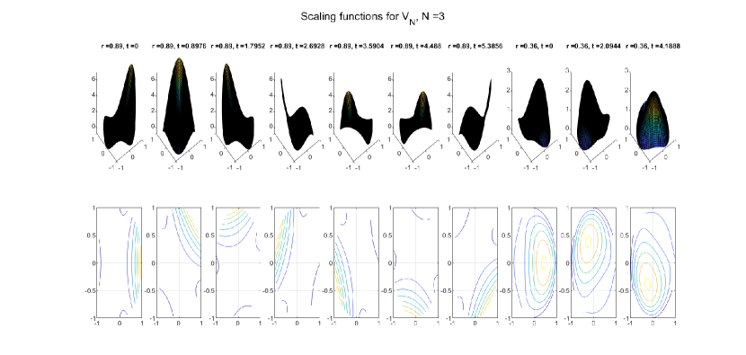
Figure 1. The surfaces and contour lines of the scaling functions for $V_{3}$.

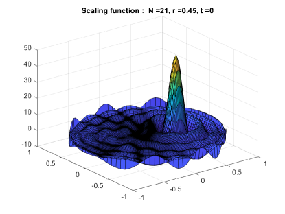
Figure 2. The surface of a scaling function for $V_{21}$.

The scaling functions for $N=3$ are shown in Figure 1. The values of $r$ and $t$ in the figure represent the values of $\rho$ and $\theta,$ respectively, corresponding to each scaling function, with $t$ being in radians and between zero and $2\pi.$ The localized nature of the scaling functions in not evident in Figure 1 due to the fact that the value of the maximum degree $N$ of polynomials considered there is too small. For higher values of $N$, one can clearly see that the scaling functions are localized. This is shown in Figure 2 for one scaling function when $N=21$ at $t=0$ and $r=.45,$ which are the values of $\theta$ and $\rho,$ respectively.

3. Wavelets

In this section, we define wavelets in terms of kernel polynomials and present some of their properties. For $N\in\mathbb{N},$ let $J_{N}=\frac{(N+1)(N+2)}{2}.$ Consider the sequence of spaces $\{V_{N}\}_{N=0}^{\infty}$ where, using Corollary 2.2 and Theorem 2.6 (iii),

$$V_{N}=\textrm{span}\{Z^{m}_{n}\}_{\begin{subarray}{c}n=0,|m|\leq n\\ (n-m)\textrm{even}\end{subarray}}^{N}=\textrm{span}\{\phi_{N,j}\}_{j=1}^{J_{N}}.$$

Note that in $\{\phi_{N,j}\}_{j=1}^{J_{N}},$ where $\phi_{N,j}=K_{N}(r,\phi;\rho^{(N)}_{j},\theta_{j}^{(N)}),$ we are considering a set of regular points $\{\rho^{(N)}_{j},\theta_{j}^{(N)})\}_{j=1}^{J_{N}}$ as described in Definition 2.4 with $J_{N}$ replaced by $J$ in the notation. Let

$$W_{N}:=V_{2N}\ominus V_{N}=\textrm{span}\{Z^{m}_{n}\}_{\begin{subarray}{c}n=N+1,|m|\leq n\\ (n-m)\textrm{even}\end{subarray}}^{2N}=\textrm{span}\{x^{\alpha}:N<|\alpha|\leq 2N,\alpha\in\mathbb{N}_{0}^{2}\}.$$

The dimension of $W_{N}$ is

$$D_{N}:=\textrm{dim}(W_{N})=\textrm{dim}(V_{2N})-\textrm{dim}(V_{N})=\frac{(2N+1)(2N+2)}{2}-\frac{(N+1)(N+2)}{2}=\frac{3N(N+1)}{2}.$$

Our target functions, called wavelets, that we wish to form a localized basis for the space $W_{N}$ are defined in polar form as

$$\psi_{N,j}(r,\phi) :=K_{2N}(r,\phi;\mu_{j}^{(N)},\omega_{j}^{(N)})-K_{N}(r,\phi;\mu_{j}^{(N)},\omega_{j}^{(N)})$$

(3.1) $$=\sum_{n=N+1}^{2N}\sum_{\begin{subarray}{c}m=-n\\ (n-m)\textrm{even}\end{subarray}}^{n}\overline{Z^{m}_{n}(\mu_{j}^{(N)},\omega_{j}^{(N)})}Z_{n}^{m}(r,\phi),\quad j=1,\ldots,D_{N},$$

(3.2) $$=\sum_{\ell=J_{N}+1}^{J_{2N}}\overline{Z_{\ell}(\mu_{j}^{(N)},\omega_{j}^{(N)})}Z_{\ell}(r,\phi),\quad j=1,\ldots,D_{N},$$

for a suitable set of points $\{\mu^{(N)}_{j},\omega_{j}^{(N)})\}_{j=1}^{D_{N}}.$

Some properties of the wavelets defined in (3.1) are now given.

Theorem 3.1.

Let $\{\psi_{N,j}(r,\phi)\}_{j=1}^{D_{N}}$ be the wavelets as defined in (3.1) with respect to the set $\{(\mu^{(N)}_{j},\omega_{j}^{(N)})\}_{j=1}^{D_{N}}.$ Then the following hold.

1. $$\langle\psi_{N,j}(r,\phi),\psi_{N,k}(r,\phi)\rangle=\psi_{N,k}(\mu^{(N)}_{j},\omega_{j}^{(N)}).$$

2. The wavelet $\psi_{N,j}$ is localized around $(\mu^{(N)}_{j},\omega_{j}^{(N)})$ i.e.,

   $$\left\|\frac{\psi_{N,j}(r,\phi)}{\psi_{N,j}(\mu^{(N)}_{j},\omega_{j}^{(N)})}\right\|=\min\{\|\psi\|:\psi\in W_{N},\psi(\mu^{(N)}_{j},\omega_{j}^{(N)})=1\}.$$

3. Let $J=\frac{(N+1)(N+2)}{2}.$ Let $\{\phi_{N,j}\}_{j=1}^{J}$ be the set of scaling functions in $V_{N}$ based on the set of points $\{\rho^{(N)}_{j},\theta_{j}^{(N)}\}_{j=1}^{J}.$ Then the wavelets and scaling functions are orthogonal, i.e.,

   $$\langle\psi_{N,j},\phi_{N,k}\rangle=0,\quad j,k=1,\ldots,J.$$

Proof.

1. $$\langle\psi_{N,j}(r,\phi),\psi_{N,k}(r,\phi)\rangle =\left\langle K_{2N}(\cdot,\cdot;\mu_{j}^{(N)},\omega_{j}^{(N)})-K_{N}(\cdot,\cdot;\mu_{j}^{(N)},\omega_{j}^{(N)}),\psi_{N,k}(\cdot,\cdot)\right\rangle$$

   (3.3) $$=\left\langle K_{2N}(\cdot,\cdot;\mu_{j}^{(N)},\omega_{j}^{(N)}),\psi_{N,k}(\cdot,\cdot)\right\rangle-\left\langle K_{N}(\cdot,\cdot;\mu_{j}^{(N)},\omega_{j}^{(N)}),\psi_{N,k}(\cdot,\cdot)\right\rangle$$

   Due to the reproducing property of the kernel polynomial, the first term on the right of (3.3) is equal to $\psi_{N,k}(\mu_{j}^{(N)},\omega_{j}^{(N)}).$ The second term on the right of (3.3) is zero due to orthogonality of the Zernike polynomials. Thus we have

   $$\langle\psi_{N,j}(r,\phi),\psi_{N,k}(r,\phi)\rangle=\psi_{N,k}(\mu_{j}^{(N)},\omega_{j}^{(N)})$$

   as needed.

2. The proof is identical to the proof of Lemma 2.3.

3. $$\langle\psi_{N,j},\phi_{N,k}\rangle =\left\langle K_{2N}(\cdot,\cdot;\mu_{j}^{(N)},\omega_{j}^{(N)})-K_{N}(\cdot,\cdot;\mu_{j}^{(N)},\omega_{j}^{(N)}),K_{N}(\cdot,\cdot;\rho_{k}^{(N)},\theta_{k}^{(N)})\right\rangle$$

   $$=\left\langle\sum_{n=N+1}^{2N}\sum_{\begin{subarray}{c}m=-n\\ (n-m)\textrm{even}\end{subarray}}^{n}\overline{Z^{m}_{n}(\mu_{j}^{(N)},\omega_{j}^{(N)})}Z_{n}^{m}(r,\phi),\sum_{n=0}^{N}\sum_{\begin{subarray}{c}m=-n\\ (n-m)\textrm{even}\end{subarray}}^{n}\overline{Z^{m}_{n}(\rho_{k}^{(N)},\theta_{k}^{(N)})}Z_{n}^{m}(r,\phi)\right\rangle$$

   $$=0$$

   due to orthogonality of the Zernike polynomials.

∎

For an arbitrary set of points, one cannot expect $\{\psi_{N,j}(r,\phi)\}_{j=1}^{D_{N}}$ to be linearly independent. However, the following can be established regarding linear independence.

Theorem 3.2 (Linear independence of wavelet functions).

For a set of points $\{(\rho_{j},\theta_{j})\}_{j=1}^{D_{N}}$ where $D_{N}=\frac{3N(N+1)}{2}$ consider the set of wavelet functions

$$\psi_{N,j}(r,\phi)=K_{2N}(r,\phi;\rho_{j},\theta_{j})-K_{N}(r,\phi;\rho_{j},\theta_{j}).$$

If the points $\{(\rho_{j},\theta_{j})\}_{j=1}^{D_{N}}$ are chosen according to Definition 2.4 by setting $N=2N$ there, and considering any subset of $D_{N}$ points, then the set $\{\psi_{N,j}(r,\phi)\}_{j=1}^{D_{N}}$ will form a basis of $W_{N}.$

Proof.

Since the number of elements in $\{\psi_{N,j}(r,\phi)\}_{j=1}^{D_{N}}$ is the same as the dimension of $W_{N}$, it is enough to show that this set of linearly independent. Following the notation in (3.2),

$$\psi_{N,j}(r,\phi)=\sum_{\ell=J_{N}+1}^{J_{2N}}\overline{Z_{\ell}(\rho_{j},\theta_{j})}Z_{\ell}(r,\phi)$$

which can be written in matrix form as

$$\begin{bmatrix}\psi_{N,1}\\ \psi_{N,2}\\ \vdots\\ \psi_{N,D_{N}}\end{bmatrix}=\begin{bmatrix}\overline{Z_{J_{N}+1}}(\rho_{1},\theta_{1})&\overline{Z_{J_{N}+2}}(\rho_{1},\theta_{1})&\cdots&\overline{Z_{J_{2N}}}(\rho_{1},\theta_{1})\\ \overline{Z_{J_{N}+1}}(\rho_{2},\theta_{2})&\overline{Z_{J_{N}+2}}(\rho_{2},\theta_{2})&\cdots&\overline{Z_{J_{2N}}}(\rho_{2},\theta_{2})\\ \vdots&\vdots&\cdots&\vdots\\ \overline{Z_{J_{N}+1}}(\rho_{D_{N}},\theta_{D_{N}})&\overline{Z_{J_{N}+2}}(\rho_{D_{N}},\theta_{D_{N}})&\cdots&\overline{Z_{J_{2N}}}(\rho_{D_{N}},\theta_{D_{N}})\\ \end{bmatrix}\begin{bmatrix}Z_{J_{N}+1}\\ Z_{J_{N}+2}\\ \vdots\\ Z_{J_{2N}}\end{bmatrix}$$

or,

(3.4) $$\begin{bmatrix}\psi_{N,1}\\ \psi_{N,2}\\ \vdots\\ \psi_{N,D_{N}}\end{bmatrix}=C_{N}\begin{bmatrix}Z_{J_{N}+1}\\ Z_{J_{N}+2}\\ \vdots\\ Z_{J_{2N}}\end{bmatrix}$$

where $C_{N}=A_{N}^{*}$ and

$$A_{N}=[Z_{J_{N}+i}(\rho_{j},\theta_{j})]_{1\leq i,j\leq D_{N}}.$$

Suppose that

$$a_{1}\psi_{N,1}+a_{2}\psi_{N,2}+\cdots+a_{D_{N}}\psi_{N,D_{N}}=0.$$

Then

$$0=\begin{bmatrix}a_{1}&a_{2}&\cdots&a_{D_{N}}\end{bmatrix}\begin{bmatrix}\psi_{N,1}\\ \psi_{N,2}\\ \vdots\\ \psi_{N,D_{N}}\end{bmatrix}=\begin{bmatrix}a_{1}&a_{2}&\cdots&a_{D_{N}}\end{bmatrix}C_{N}\begin{bmatrix}Z_{J_{N}+1}\\ Z_{J_{N}+2}\\ \vdots\\ Z_{J_{2N}}\end{bmatrix}.$$

This implies,

$$\begin{bmatrix}\overline{Z_{J_{N}+1}}&\overline{Z_{J_{N}+2}}&\cdots&\overline{Z_{J_{2N}}}\end{bmatrix}A_{N}\begin{bmatrix}a_{1}\\ a_{2}\\ \vdots\\ a_{D_{N}}\end{bmatrix}=0$$

or,

$$A_{N}\begin{bmatrix}a_{1}\\ a_{2}\\ \vdots\\ a_{D_{N}}\end{bmatrix}=0.$$

Due to the choice of $\{(\rho_{j},\theta_{j})\}_{j=1}^{D_{N}},$ the matrix $A_{N}$ is non-singular [13]. Thus, the only possibility is

$$a_{1}=a_{2}=\cdots=a_{D_{N}}=0,$$

and the set $\{\psi_{N,j}\}_{j=1}^{D_{N}}$ is linearly independent. ∎

Figure 3 shows points, taken according to Definition 2.4 and Theorem 3.2, for the scaling functions and the wavelets, respectively, when $N=3.$ A few wavelet functions constructed by (3.1) are shown in Figure 4. The values of $r$ and $t$ shown in Figure 4 represent the values of $\rho$ and $\theta$, respectively, corresponding to each wavelet function, with $t$ being in radians.

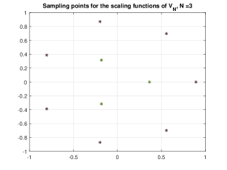
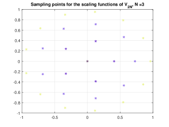
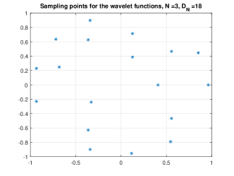
Figure 3. Points used for the scaling functions, $N=3$.

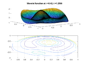
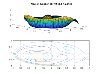
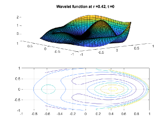
Figure 4. Surfaces and contour lines of some wavelet functions, $N=3$.

4. Dual functions

It may not be possible to get orthogonal wavelets from Theorem 3.2. In that case, in order to reconstruct any signal, one needs to find the dual of the wavelet basis. We illustrate a method of finding a matrix representation for the dual.

Consider the wavelet basis $\{\psi_{N,j}(r,\phi)\}_{j=1}^{D_{N}}$ of $W_{N}$ as shown in Theorem 3.2. Take $f\in W_{N}.$ Denote the dual of the wavelet basis by $\{\widetilde{\psi}_{N,j}(r,\phi)\}_{j=1}^{D_{N}}.$ Then $f$ can be written as

$$f=\sum_{j=1}^{D_{N}}\langle f,\psi_{N,j}\rangle\widetilde{\psi}_{N,j}.$$

Due to Corollary 2.2, we know that $\{Z_{\ell}(r,\phi)\}_{\ell=J_{N}+1}^{J_{2N}}$ is an ONB for $W_{N}=V_{2N}\ominus V_{N}.$ In terms of this ONB, the function $f$ can be written as

$$f=\sum_{\ell=J_{N}+1}^{J_{2N}}f^{(\ell)}Z_{\ell}(r,\phi).$$

Let us identify $f$ with the vector $[f^{(J_{N}+1)}\ \ldots\ f^{(J_{2N})}]^{\textrm{\tiny{T}}}.$ Recall that the $j$th wavelet function is

(4.1) $$\psi_{N,j}(r,\phi)=\sum_{\ell=J_{N}+1}^{J_{2N}}\overline{Z_{\ell}(\rho_{j},\theta_{j})}Z_{\ell}(r,\phi)$$

where the set of points $\{(\rho_{j},\theta_{j})\}_{j=1}^{D_{N}}$ is chosen in a manner outlined in Theorem 3.2 so that $\{\psi_{N,j}(r,\phi)\}_{j=1}^{D_{N}}$ is a linearly independent set. We identify $\psi_{N,j}(r,\phi)$ with the vector $[Z_{J_{N}+1}(\rho_{j},\theta_{j})\ Z_{J_{N}+2}(\rho_{j},\theta_{j})\ \ldots\ Z_{2J_{N}}(\rho_{j},\theta_{j})]^{*}$ where $*$ represents the complex conjugate transpose. Consider the matrix

$$B_{N}=\begin{bmatrix}\overline{Z_{J_{N}+1}}(\rho_{1},\theta_{1})&\overline{Z_{J_{N}+1}}(\rho_{2},\theta_{2})&\cdots&\overline{Z_{J_{N}+1}}(\rho_{D_{N}},\theta_{D_{N}})\\ \overline{Z_{J_{N}+2}}(\rho_{1},\theta_{1})&\overline{Z_{J_{N}+2}}(\rho_{2},\theta_{2})&\cdots&\overline{Z_{J_{N}+2}}(\rho_{D_{N}},\theta_{D_{N}})\\ \vdots&\vdots&\vdots&\vdots\\ \overline{Z_{J_{2N}}}(\rho_{1},\theta_{1})&\overline{Z_{J_{2N}}}(\rho_{2},\theta_{2})&\cdots&\overline{Z_{J_{2N}}}(\rho_{D_{N}},\theta_{D_{N}})\end{bmatrix}.$$

Note that the $j$th column of $B_{N}$ represents the $j$th wavelet function $\psi_{N,j}.$ In vector notation, it can be seen that

$$B_{N}^{*}f=\begin{bmatrix}\langle f,\psi_{N,1}\rangle\\ \langle f,\psi_{N,2}\rangle\\ \vdots\\ \langle f,\psi_{N,D_{N}}\rangle\\ \end{bmatrix}.$$

Therefore,

$$B_{N}B_{N}^{*}f =\begin{bmatrix}\overline{Z_{J_{N}+1}}(\rho_{1},\theta_{1})&\overline{Z_{J_{N}+1}}(\rho_{2},\theta_{2})&\cdots&\overline{Z_{J_{N}+1}}(\rho_{D_{N}},\theta_{D_{N}})\\ \overline{Z_{J_{N}+2}}(\rho_{1},\theta_{1})&\overline{Z_{J_{N}+2}}(\rho_{2},\theta_{2})&\cdots&\overline{Z_{J_{N}+2}}(\rho_{D_{N}},\theta_{D_{N}})\\ \vdots&\vdots&\vdots&\vdots\\ \overline{Z_{J_{2N}}}(\rho_{1},\theta_{1})&\overline{Z_{J_{2N}}}(\rho_{2},\theta_{2})&\cdots&\overline{Z_{J_{2N}}}(\rho_{D_{N}},\theta_{D_{N}})\end{bmatrix}\begin{bmatrix}\langle f,\psi_{N,1}\rangle\\ \langle f,\psi_{N,2}\rangle\\ \vdots\\ \langle f,\psi_{N,D_{N}}\rangle\\ \end{bmatrix}$$

$$=\langle f,\psi_{N,1}\rangle\begin{bmatrix}\overline{Z_{J_{N}+1}}(\rho_{1},\theta_{1})\\ \overline{Z_{J_{N}+2}}(\rho_{1},\theta_{1})\\ \vdots\\ \overline{Z_{J_{2N}}}(\rho_{1},\theta_{1})\end{bmatrix}+\cdots+\langle f,\psi_{N,D_{N}}\rangle\begin{bmatrix}\overline{Z_{J_{N}+1}}(\rho_{D_{N}},\theta_{D_{N}})\\ \overline{Z_{J_{N}+2}}(\rho_{D_{N}},\theta_{D_{N}})\\ \vdots\\ \overline{Z_{J_{2N}}}(\rho_{D_{N}},\theta_{D_{N}})\end{bmatrix}$$

$$=\sum_{r=1}^{D_{N}}\langle f,\psi_{N,r}\rangle\psi_{N,r}$$

$$\implies f =\sum_{r=1}^{D_{N}}\langle f,\psi_{N,r}\rangle(B_{N}B_{N}^{*})^{-1}\psi_{N,r}=\sum_{r=1}^{D_{N}}\langle f,(B_{N}B_{N}^{*})^{-1}\psi_{N,r}\rangle\psi_{N,r}$$

$$\implies\widetilde{\psi}_{N,r} =(B_{N}B_{N}^{*})^{-1}\psi_{N,r}.$$

Since the points $\{(\rho_{j},\theta_{j})\}_{j=1}^{D_{N}}$ are chosen so that the corresponding wavelet set $\{\psi_{N,j}\}_{j=1}^{D_{N}}$ is a basis, it is guaranteed that the matrix $B_{N}B_{N}^{*}$ is invertible. The wavelet functions $\{\psi_{N,r}(r,\phi)\}_{r=1}^{D_{N}}$ form an orthonormal set if and only if $B_{N}^{*}B_{N}$ is a diagonal matrix. Since this may not be possible for the choice of points used to construct the wavelets, one has to compute $(B_{N}B_{N}^{*})^{-1}$ and then the dual $\{\widetilde{\psi}_{N,r}(r,\phi)\}_{r=1}^{D_{N}}$ to reconstruct $f$ from the wavelet coefficients $\{\langle f,\psi_{N,r}\rangle\}_{r=1}^{D_{N}}.$

Another way to think about dual functions of wavelets in matrix or vector form is the following. In the expression given in (4.1), let us consider sampling each function $\psi_{N,j}$ at $D$ points. This in turn implies that we are sampling each Zernike polynomial $Z_{\ell}(r,\phi)$ at $D$ points so that each Zernike polynomial $Z_{\ell}(r,\phi)$ can be thought of as a vector of $D$ elements. Equation (4.1) can then be written as

$$\psi_{N,j}(r,\phi) = \overline{Z_{J_{N}+1}}(\rho_{j},\theta_{j})Z_{J_{N}+1}(r,\phi)+\cdots+\overline{Z_{J_{2N}}}(\rho_{j},\theta_{j})Z_{J_{2N}}(r,\phi)$$

$$= \begin{bmatrix}|&|&\cdots&|\\ Z_{J_{N}+1}&Z_{J_{N}+2}&\cdots&Z_{J_{2N}}\\ |&|&\cdots&|\end{bmatrix}\begin{bmatrix}\overline{Z_{J_{N}+1}}(\rho_{j},\theta_{j})\\ \vdots\\ \overline{Z_{J_{2N}}}(\rho_{j},\theta_{j})\end{bmatrix}$$

$$= B\begin{bmatrix}\overline{Z_{J_{N}+1}}(\rho_{j},\theta_{j})\\ \vdots\\ \overline{Z_{J_{2N}}}(\rho_{j},\theta_{j})\end{bmatrix}.$$

Note that $B$ is a $D\times D_{N}$ matrix. Let $\Psi$ be the matrix whose $j$th column is $\psi_{N,j}.$

$$\Psi=\begin{bmatrix}|&|&\cdots&|\\ \psi_{N,1}&\psi_{N,2}&\cdots&\psi_{N,D_{N}}\\ |&|&\cdots&|\end{bmatrix}.$$

Therefore,

(4.2) $$\Psi=B\begin{bmatrix}\overline{Z_{J_{N}+1}}(\rho_{1},\theta_{1})&\cdots&\overline{Z_{J_{N}+1}}(\rho_{D_{N}},\theta_{D_{N}})\\ \vdots&\cdots&\vdots\\ \overline{Z_{J_{2N}}}(\rho_{1},\theta_{1})&\cdots&\overline{Z_{J_{2N}}}(\rho_{D_{N}},\theta_{D_{N}})\end{bmatrix}=B\ Q.$$

In the language of frame theory, the $D\times D_{N}$ matrix $\Psi$ is the synthesis operator of the discretized set of vectors $\{\psi_{N,j}\}_{j=1}^{D_{N}},$ and $\Psi\Psi^{*}$ is the frame operator [3]. The dual wavelet functions, in discretized form, are then given by

$$\widetilde{\psi}_{N,j}=(\Psi\Psi^{*})^{-1}\psi_{N,j}=(BQQ^{*}B^{*})^{-1}\psi_{N,j}.$$

5. Multiresolution Analysis

The scaling functions defined in Section 2 give rise to a multiresolution analysis (MRA) that is different from the traditional MRA. Recall that $V_{N}$ is the subspace of all polynomials in $x,$ $y$ with degree at most $N$. This gives a one-sided MRA starting with $V_{0}$ that satisfies the following.

1. $V_{2^{j}}\subset V_{2^{j+1}},$ $j\in\mathbb{N}_{0},$ giving rise to the sequence of nested subspaces starting with $V_{0}$:

   $$V_{0}\subset V_{1}\subset\cdots\subset V_{2^{j}}\subset V_{2^{j+1}}\subset\cdots.$$

2. $\bigcap_{j\in\mathbb{N}_{0}}V_{2^{j}}=V_{0}=\textrm{span}\{\mathds{1}_{B(0,1)}\}$ where $\mathds{1}_{B(0,1)}$ is the characteristic function of $B(0,1).$

3. $\overline{\bigcup_{j\in\mathbb{N}_{0}}V_{2^{j}}}=L^{2}(B(0,1)).$

4. Dilation: $p(x,y)\in V_{2^{j}}\Leftrightarrow p(x^{2},y^{2})\in V_{2^{j+1}}$
   $f\in V_{n}\Leftrightarrow\langle f,Z^{m}_{k}\rangle=0$ for all $k>n.$

5. Translation: $\{\phi_{N,r}\}_{r=1}^{J}$ based on a parameter set of special points (Definition 2.4) is a basis of $V_{N}$ where $N=2^{j}$ for some $j\in\mathbb{N}_{0}$ and $J=\frac{(N+1)(N+2)}{2}.$

The last property determined by the choice of the special points takes the role of integer translates in a standard MRA. For a given function $f$ and a given $N$ that is a power of $2$, one can obtain the best approximation of $f$ in the space $V_{N}$ by considering the orthogonal projection of $f$ on $V_{N}.$ Call this $f_{P_{N}}.$ We can write

(5.1) $$V_{N}=V_{\frac{N}{2}}\oplus W_{\frac{N}{2}}=V_{\frac{N}{4}}\oplus W_{\frac{N}{4}}\oplus W_{\frac{N}{2}}=\cdots=V_{0}\oplus W_{0}\oplus\cdots\oplus W_{\frac{N}{2}}.$$

Note that $V_{0}$ is spanned by constant polynomials and the wavelet functions form a basis for the spaces $W_{j}.$ Thus (5.1) implies that one can write $f_{P_{N}}$ as a linear combination of the wavelets. Taking higher values of $N$ will make $f_{P_{N}}$ a better approximation of $f.$

6. Numerical results and discussion

In this section we show some experimental results that demonstrate the use of wavelets constructed using Zernike polynomials. The data used comes from normal subjects, those with corneal astigmatism, and those with keratoconus. A Medmont E300 videokeratoscope was used to obtain the data. The data points for each subject are stored as a vector $C$ of size $D.$ For the data used, $D=10200.$ This data, taken from the right eye of a subject with astigmatism, is shown on the top left of Figure 5. To represent this data as an approximation in some $V_{N},$ in terms of Zernike polynomials, we first fix $N.$ For a given $N,$ there are $J=(N+1)(N+2)/2$ Zernike polynomials with radial degree at most $N$ that form a basis of $V_{N}.$ We can write [7]

$$C=Ba,$$

where $B$ is a $D\times J$ matrix whose columns are the $J$ Zernike polynomials (sampled at the $D$ points), and $a$ is a vector of coefficients. Then, using the method of least-squares, the coefficient vector $a$ can be estimated as

$$\widehat{a}=(B^{\textrm{\tiny{T}}}B)^{-1}B^{\textrm{\tiny{T}}}C.$$

Then the approximation of the data $C$ in the space $V_{N}$ is

$$\widehat{C}=B\widehat{a}.$$

To start with, we take $N=8,$ and note that any other power of $2$ can be taken; the higher the power, the better the approximation. The approximation of the elevation data $C$ in the space $V_{8}$ is shown on the top right of Figure 5. Next, we do the same with $N$ replaced by $\frac{N}{2},$ i.e., $4$ in this case. This gives an approximation of $C$ in the space $V_{4}.$ The difference between the two levels of approximation will belong to the space $W_{\frac{N}{2}}$ which is $W_{4}$. These are shown in the bottom row of Figure 5.

Using the above idea, for a given $N$ that is a power of $2$, one can obtain approximations in the spaces $V_{N},$ $V_{\frac{N}{2}},$ $V_{\frac{N}{4}},$ and so on. We can write

(6.1) $$V_{N}=V_{\frac{N}{2}}\oplus W_{\frac{N}{2}}=V_{\frac{N}{4}}\oplus W_{\frac{N}{4}}\oplus W_{\frac{N}{2}}=\cdots=V_{0}\oplus W_{0}\oplus\cdots\oplus W_{\frac{N}{2}}.$$

Note that $V_{0}$ is spanned by constant polynomials, and the choice of $N=8$ gives $J=45$ which is the dimension of the subspace $V_{8}$ as well as the number of Zernike polynomials used to represent $V_{8}.$ This means that the matrix $B$ above is of size $10200\times 45$. The dimension of the subspace $V_{4}$ is $15$ and so the wavelet space $W_{4}$ is of dimension $45-15=30.$ The next step is to represent the differences in the $W_{j}$s, i.e., the wavelets spaces, in terms of the wavelet basis functions constructed in Section 3. The points needed to construct the wavelet basis functions for $W_{j}$ is taken to be a random subset of the special points used to construct scaling functions for $V_{2j}$ as given in Definition 2.4, and discussed in Theorem 3.2. As indicated by (6.1), we can then represent our approximation in the space $V_{N},$ for a given $N,$ in terms of the wavelet functions only. Including the constant function needed for $V_{0}$ the number of wavelet functions needed for $N=8$ would also be $45.$ The reconstruction of the elevation data of Figure 5 using wavelet functions, the Zernike coefficients, and the wavelet coefficients are shown in Figure 6. The bottom row in Figure 6 shows the wavelet coefficients (left) and the difference of the same elevation data of Figure 5 with the best-fit-sphere of that data (right). The difference with the best-fit-sphere (BFS) indicates the ridges and undulations in the data. By looking at the wavelet coefficients one can determine the locations where the data changes with higher frequencies. The norm of the difference between the elevation data and the approximation using Zernike polynomials as well as using wavelet functions is $0.07.$

Similar experiments have been performed with data from the right eyes of normal subjects and subjects with keratoconus using $N=8$. An example of each is shown in Figures 7 - 10. The norm of the difference between the elevation data and the approximation using Zernike polynomials as well as using wavelet functions is $0.0682$ in normal case. The norm of the difference between the elevation data and the approximation using Zernike polynomials as well as using wavelet functions is $0.1006$ for the subject with keratoconus. One would expect better results giving more information when $N$ is larger. For $N=16$ the dimension of $V_{16}$ is $153$ which is the same as the number of wavelet functions to be used for this value of $N.$ See Figure 11 for the subject with astigmatism discussed earlier in Figure 5 and Figure 6. Now there are many more wavelet coefficients and consequently one has a better knowledge of locations of fluctuations in spatial frequency. The norm of the difference between the elevation data and the approximation using Zernike polynomials as well as using wavelet functions is now $0.05.$ In comparing the wavelet coefficients obtained from $N=8$ and $N=16,$ it is worth recalling that the wavelet functions for $W_{N}$ are constructed from a random subset of points that are used to construct the scaling functions for $V_{2N}$. Each trial, with a given data set and a particular $N,$ uses a different set of wavelets functions, and this will also effect the location of the most significant wavelet coefficients. What is seen in Figures 6, 8, 10, and 11 is just from a single trial. However, one can see that for the same astigmatism data with $N=8$ and $N=16,$ the one for $N=16$ (Figure 11) has a lot more wavelet coefficients and hence gives much more information than the corresponding result for $N=8$ (Figure 6). The difference between two different trials will be less noticeable as $N$ increases and more and more points are used. The results will be more meaningful with higher values of $N$ at the cost of more computational time.

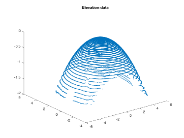
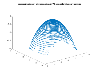
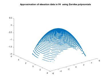
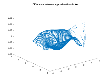
Figure 5. Approximation of elevation data of a subject with astigmatism.

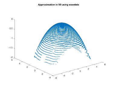
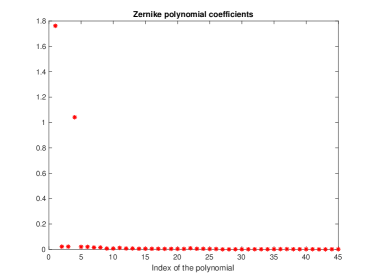
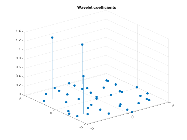
Figure 6. Wavelet and Zernike coefficients of the astigmatism data of Figure 5

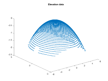
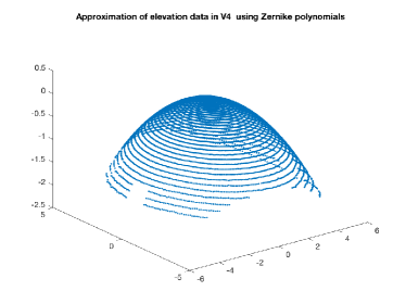
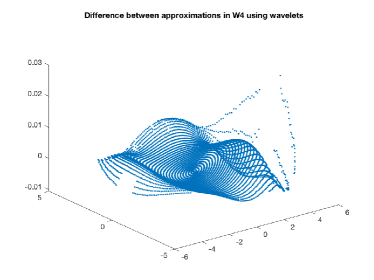
Figure 7. Approximation of elevation data of a normal subject.

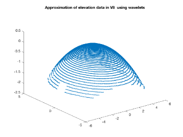
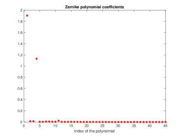
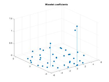
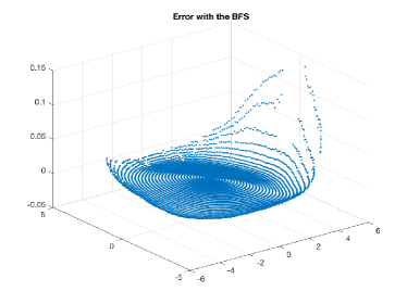
Figure 8. Wavelet and Zernike coefficients of the data from a normal subject of Figure 7

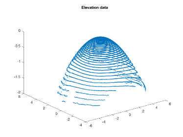
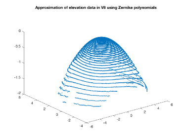
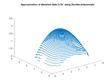
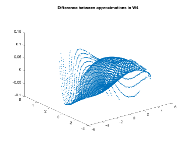
Figure 9. Approximation of elevation data of a subject with keratoconus.

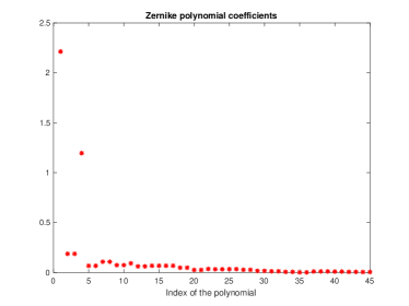
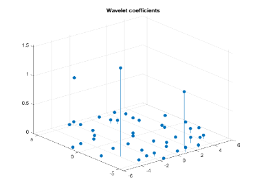
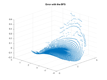
Figure 10. Wavelet and Zernike coefficients of the data from a subject with keratoconus of Figure 9

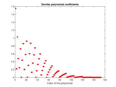
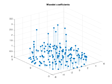
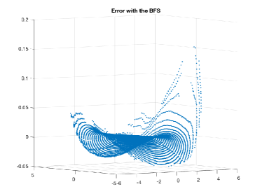
Figure 11. Wavelet and Zernike coefficients of the astigmatism data of Figure 5 using $N=16$

7. Acknowledgments

The authors are immensely grateful to Dr. D. Robert Iskander for providing the data used for experimental results in this work. The first named author would like to acknowledge support from Simons Foundation under Award No. 709212.

References

- [1]
- [2] L. Bos. Near optimal location of points for Lagrange interpolation in several variables. Ph.D. thesis, University of Toronto, 1981.
- [3] O. Christensen An Introduction to Frames and Riesz Bases. Birkhäuser, Boston, Second Edition, Applied and Numerical Harmonic Analysis series, 2016.
- [4] B. Fischer and J. Prestin. Wavelets based on orthogonal polynomials. Mathematics of Computation. Vol. 66, No. 220, 1593 – 1618, 1997.
- [5] K. Gröchenig and W. Madych. Multiresolution analysis, Haar bases, and self-similar tilings of IEEE Transactions on Information Theory. Vol. 38, 556 – 568, 1992.
- [6] A. Haar. Zur Theorie der Orthogonalen Functionen-Systeme. Math. Ann. Vol. 69, 331 – 371, 1910.
- [7] D. R. Iskander, M. R. Morelande, M. J. Collins, and B. Davis. Modeling of corneal surfaces with radial polynomials. IEEE Transactions on Biomedical Engineering. Vol. 49, no. 4, 320 – 328, April 2002. doi: 10.1109/10.991159.
- [8] T. Kilgore and J. Prestin. Polynomial wavelets on the interval. Constructive Approximation. Vol. 12, 95 – 110, 1996.
- [9] W. Madych. Some elementary properties of multiresolution analyses of in Wavelets: A Tutorial in Theory and Applications Vol II, edited by C. Chui. Academic Press, Inc., 259 – 294, 1992.
- [10] S. Mallat. Multiresolution approximations and wavelet orthonormal bases for . Trans. Amer. Math. Soc. Vol. 315, 69 – 87, 1989.
- [11] Y. Meyer. Wavelets: Algorithms & applications. Translated from French and with a foreword by Robert D. Ryan. SIAM, Philadelphia, 1993.
- [12] B. R. A. Nijboer. The Diffraction Theory of Aberrations. Ph.D. Thesis, University of Groningen, 1942. Also, Physica (23), 605–620, 1947.
- [13] D. Ramos-López, M. A. Sánchez-Granero, and M. Fernández-Martínez. Optimal sampling patterns for Zernike polynomials. Applied Mathematics and Computation. Vol. 274, 247 – 257, 2016.
- [14] Y. Xu. Lecture notes on orthogonal polynomials of several variables. Advances in the Theory of Special Functions and Orthogonal Polynomials. Nova Science Publishers. Vol. 2, 135 – 188, 2004.
- [15] F. Zernike. Beugungstheorie des schneidenver-fahrens und seiner verbesserten form, der phasenkontrastmethode. Physica. Vol. 1 (7-12), 689 – 704, 1934.