Multiresolution of the one dimensional free-particle propagator

Abstract.

Novel methods to integrate the time-dependent Schrödinger equation within the framework of multiscale approximation is presented. The methods are based on symplectic splitting algorithms to separate the kinetic and potential parts of the corresponding propagator. The semigroup associated with the free-particle Schrödinger operator is represented in a multiwavelet basis. The propagator is effectively discretized with a contour deformation technique, which overcomes the challenges presented by previous discretization methods. The discretized operator is then employed in simple numerical simulations to test the validity of the implementation and to benchmark its precision.

1. Introduction

Let us consider the one-dimensional time-dependent Schrödinger equation

$$i\partial_{t}u=-\partial_{x}^{2}u+V(x,t)u,$$ (1.1)

complemented by the initial condition given at $t=0$ by

$$u(0)=u_{0}\in L^{2}(\mathbb{R}).$$ (1.2)

The space variable $x\in\mathbb{R}$ and the time variable $t>0$. In general a real-valued potential $V(x,t)$ can depend on the solution, as for example, in water waves and Hartree-Fock theories.

The main objective of this work is to provide an effective numerical discretization of the exponential operator $\exp\left(it\partial_{x}^{2}\right),$ where $t\in\mathbb{R}$ is a small parameter, not necessarily positive. In what follows we assume that $t\neq 0$. Our goal is to construct a numerical representation of this operator to solve Equation (1.1) adaptively. It is known that a use of multiwavelet bases [6] may lead to adaptive numerical solutions for some partial differential equations [7]. However, the time-evolution operator $\exp\left(it\partial_{x}^{2}\right)$ falls outside this operator class, that are known to give sparse representations in this type of bases [9, 21]. Nevertheless, it turns out that $\exp\left(it\partial_{x}^{2}\right)$ exhibits a unique peculiarity that can be leveraged in adaptive calculations, as we demonstrate below.

We recall that the $t$-dependent exponential operator under consideration here forms a semigroup representing solutions of the free particle equation

$$i\partial_{t}u+\partial_{x}^{2}u=0.$$ (1.3)

In other words, for any square integrable $u_{0}\in L^{2}(\mathbb{R})$, the function $u=\exp\left(it\partial_{x}^{2}\right)u_{0}$ solves Equation 1.3. In numerical simulations, the parameter $t$ usually plays the role of a time (sub)step. The importance of an effective discretization of this exponential operator, at least for a time-independent potential $V$, can be exemplified as follows. Let $A,B$ be time independent linear operators. One of the simplest second-order splitting methods can be expressed as follows

$$e^{At+Bt}=e^{Bt/2}e^{At}e^{Bt/2}+\mathcal{O}\left(t^{3}\right).$$ (1.4)

Taking $A=i\partial_{x}^{2}$ and $B=-iV$, one can evolve Equation (1.1) by applying the multiplication operator $e^{Bt/2}$ twice and the pseudo-differential operator $e^{At}$ once at each time step starting from the initial function (1.2). Such operator splitting simplifies the problem (1.1), (1.2) significantly: the exponential of the multiplicative operator is straightforward and the problem reduces to finding an efficient representation for the exponential of the kinetic energy. Below we will also make use of higher order schemes than (1.4). They will permit larger time steps, which turns out to be especially crucial for multiwavelet representation of the semigroup $\exp\left(it\partial_{x}^{2}\right),$ due to some limitations on how small a time step $t$ might be taken.

We are motivated by the desire of simulating attosecond electron dynamics. In recent years there has been a growing interest in studying the electronic structure of molecules under strong and ultra-fast laser pulses [30]. This is clearly testified by the 2018 and 2023 Nobel prizes in Physics[29, 33]. This could potentially lead to reaction control by attosecond laser pulses in the future. From a computational perspective, electron dynamics in atoms and molecules is challenging: standard atomic orbital approaches routinely used in Quantum Chemistry cannot be applied in strong laser pulses, as simple numerical experiments suggest that ionization plays a significant role and cannot be neglected [17]. In other words, the coupling with continuum or unbound states complicates the use of atomic orbitals for the problem discretization. Inevitably it demands the use of grid based methods, such as finite elements, for example.

In the case of hydrogen atom subjected to a laser field we have the following three-dimensional Schrödinger equation

$$i\partial_{t}\psi=-\frac{1}{2}\Delta\psi-\frac{1}{|x|}\psi+\mathcal{E}(x,t)\psi,$$ (1.5)

where the second term $-|x|^{-1}$ stands for the Coulomb potential and $\mathcal{E}(x,t)$ stands for the external electric field generated by a laser. It is normally complemented by the ground state $\psi_{0}(x)=e^{-|x|}/\sqrt{\pi}$ serving as an initial condition $\psi(x,0)=\psi_{0}(x)$.

It can be advantageous to make use of adaptive methods to describe the singular Coulomb interaction between the electron and the nucleus, as well as the cusp in the eigenfunctions which follows from it. This, however, sets some limitations on the method development. Additionally, for many-body systems (atoms and molecules), the potential becomes nonlinear due to the presence of electron-electron interactions. The corresponding nonlinearities are normally presented in equations as singular integral convolutions. One such method is constituted by a multiwavelet (MW) representation, within the framework of multiresolution analysis [7]. This approach has demonstrated excellent results in achieving fast algorithms and high precision for static quantum chemistry problems [23, 24, 26]. However, discussing these static results is beyond the scope of the current contribution. Furthermore, the research field is rapidly evolving, and we recommend referring to a comprehensive review paper for a broader perspective [10]. An overview of the most recent advancements will also be available in an upcoming paper [37].

We aim to extend the multiwavelet approach to address time-dependent scenarios. The first step in integrating the generic time-dependent Schrödinger equation, similar to (1.5), involves discretizing the semigroup $e^{it\Delta}$. Due to the limitations highlighted above, the fast Fourier transform (FFT) cannot be relied upon for quantum chemistry applications. This is why we find the multiscale approach promising. To our knowledge, the only work on multiwavelet representation of the dynamical Shrödinger type equations was conducted by Vence et al. [38]. They view the semigroup as a convolution and mitigate the errors arising from its oscillatory behavior by damping high-frequency oscillations in Fourier space. The resulting kernel approximation can be seamlessly integrated into the multiwavelet framework developed for static problems.

In contrast, we adopt a different approach by leveraging the smoothing property of the semigroup instead of damping it. It enables us to achieve a highly accurate multiscale approximation of the free-particle propagator. Moreover, it turns out that this representation can be regarded as sparse, as long as particular restrictions are met during numerical simulations. Since we do not treat the semigroup as a convolution suitable for chemistry applications, unlike the mentioned above method employed by Vence et al., further development is necessary to fully exploit our representation for studying electron dynamics in molecules. Therefore, this article focuses exclusively on the one-dimensional case. In the future, we plan to extend our results and simulate the three-dimensional quantum mechanical problems.

The paper is organised as follows. In Section 2 we introduce some preliminary notions and recall the theory behind multiwavelet bases. In Section 3 we lay out the problem with some insights into the difficulties that we aim to overcome. In Section 4, the multiresolution representation of $\exp\left(it\partial_{x}^{2}\right)$ is reduced to the evaluation of a special kind of integrals. In Section 4 these integrals are evaluated by deforming the integration contour in a way that allows to exploit the smoothing property of this exponential operator. Furthermore, we demonstrate that by carefully selecting the time parameter $t$ and polynomial approximation order, its multiresolution representation will display an unusual sparsity pattern. More specifically, the matrices used in calculations have non-zero elements away from their main diagonals. This sparsity depends significantly on the value of $t$, necessitating the use of high-order numerical schemes for accurate wave propagation simulations. To address this requirement, we introduce high-order symplectic integrators in Section 5. Finally, we test our numerical representation of $\exp\left(it\partial_{x}^{2}\right)$ by running numerical simulations for toy benchmark models in Section 6. A summary is provided in Section 7 with some plans for future works.

2. Multiwavelet bases

This section provides a concise theoretical background on multiwavelet bases. We are interested in approximations of functions in $L^{2}(\mathbb{R})$. However, for practical reasons, we have to restrict ourselves to a sufficiently large interval. Equation (1.1) can always be normalised in such a way that the unit computational domain $[0,1]$ will suit our needs, while keeping the constant in front of the second derivative to be $-1$. Note that any function $u\in L^{2}(0,1)$ can be trivially extended to a function in $L^{2}(\mathbb{R})$, by setting it to zero outside $(0,1)$. On the contrary, any function from $L^{2}(\mathbb{R})$ can be projected into $L^{2}(0,1)$, by multiplying it with the characteristic function of the unit interval $(0,1)$. This remark allows us to make sense of the inclusion $L^{2}(0,1)\subset L^{2}(\mathbb{R}).$ Now for any $\mathfrak{k}\in\mathbb{N}=\{1,2,\ldots\}$ and any $n\in\mathbb{N}_{0}=\{0,1,2,\ldots\}$ we introduce a space of piecewise polynomials $V_{n}^{\mathfrak{k}}$ as follows. A function $f\in V_{n}^{\mathfrak{k}}$ provided that on each dyadic interval $(l/2^{n},(l+1)/2^{n})$ with $l=0,1,\ldots,2^{n}-1$ it is a polynomial of degree less than $\mathfrak{k}$ and it is zero elsewhere. Note that the space $V_{n}^{\mathfrak{k}}$ has dimension $2^{n}\mathfrak{k}$ and

$$V_{0}^{\mathfrak{k}}\subset V_{1}^{\mathfrak{k}}\subset\ldots\subset V_{n}^{\mathfrak{k}}\subset\ldots\subset L^{2}(0,1)\subset L^{2}(\mathbb{R}),$$

which defines a multiresolution analysis (MRA) [27, 28], since the union $\bigcup_{n=0}^{\infty}V_{n}^{\mathfrak{k}}$ is dense in $L^{2}(0,1)$. We refer to the given fixed number $\mathfrak{k}$ as the order of MRA and to the integer variable $n$ as a scaling level.

Let $\phi_{0},\ldots,\phi_{\mathfrak{k}-1}$ be a basis of $V_{0}^{\mathfrak{k}}$ that will be called scaling functions. The space $V_{n}^{\mathfrak{k}}$ is spanned by $2^{n}\mathfrak{k}$ functions which are obtained from the scaling functions by dilation and translation

$$\phi_{jl}^{n}(x)=2^{n/2}\phi_{j}(2^{n}x-l),\quad j=0,\ldots,\mathfrak{k}-1,\quad l=0,\ldots,2^{n}-1.$$ (2.1)

There is some freedom in choosing a basis in $V_{0}^{\mathfrak{k}}$, at least for $\mathfrak{k}>1$. The first example appeared in [6], and it consists of the Legendre scaling functions

$$\phi_{j}(x)=\sqrt{2j+1}P_{j}(2x-1),\quad x\in(0,1),\quad j=0,\ldots,\mathfrak{k}-1,$$ (2.2)

where $P_{j}$ are standard Legendre polynomials. Outside the unit interval $(0,1)$ they are set to zero. An alternative basis, proved to be more efficient that is especially crucial in multi-dimensional numerical calculations, was presented in [7]. It consists of the interpolating scaling functions

$$\varphi_{j}(x)=\sqrt{w_{j}}\sum_{m=0}^{\mathfrak{k}-1}\phi_{m}(x_{j})\phi_{m}(x),\quad j=0,\ldots,\mathfrak{k}-1,$$ (2.3)

where $\phi_{m}$ are the Legendre scaling functions (2.2). Here $x_{0},\ldots,x_{\mathfrak{k}-1}$ denote the roots of $P_{\mathfrak{k}}(2x-1)$ and the quadrature weights $w_{j}=1/(\mathfrak{k}P_{\mathfrak{k}}^{\prime}(2x_{j}-1)P_{\mathfrak{k}-1}(2x_{j}-1)).$ The expansion coefficients of a general function $f$ in a scaling basis are the integrals

$$s_{jl}^{n}(f)=\int_{\mathbb{R}}f(x)\phi_{jl}^{n}(x)dx=2^{-n/2}\int_{0}^{1}f(2^{-n}(x+l))\phi_{j}(x)dx,$$ (2.4)

that can be evaluated numerically using the Gauss-Legendre quadrature

$$s_{jl}^{n}(f)\approx 2^{-n/2}\sum_{m=0}^{\mathfrak{k}-1}w_{m}f(2^{-n}(x_{m}+l))\phi_{j}(x_{m}),\quad j=0,\ldots,\mathfrak{k}-1,\quad l=0,\ldots,2^{n}-1.$$ (2.5)

Note that the interpolating scaling functions (2.3) satisfy $\varphi_{j}(x_{m})=w_{j}^{-1/2}\delta_{jm}$ and so (2.5) simplifies to

$$s_{jl}^{n}(f)\approx 2^{-n/2}\sqrt{w_{j}}f(2^{-n}(x_{m}+l))$$ (2.6)

for this particular choice of a basis.

The multiwavelet space $W_{n}^{\mathfrak{k}}$ is defined as the orthogonal complement of $V_{n}^{\mathfrak{k}}$ in $V_{n+1}^{\mathfrak{k}}$, so we have

$$V_{n+1}^{\mathfrak{k}}=V_{n}^{\mathfrak{k}}\oplus W_{n}^{\mathfrak{k}}=V_{0}^{\mathfrak{k}}\oplus W_{0}^{\mathfrak{k}}\oplus W_{1}^{\mathfrak{k}}\oplus\ldots\oplus W_{n}^{\mathfrak{k}}.$$

As above it is enough to define a basis $\psi_{0},\ldots,\psi_{\mathfrak{k}-1}$ in $W_{0}^{\mathfrak{k}}$ and then transform it in line with the general rule (2.1), in order to get an orthonormal basis in each $W_{n}^{\mathfrak{k}}$. The construction of a specific multiwavelet basis that satisfies certain given restrictions is more involved. We are using the one that was constructed in [6], since it provides us with an additional vanishing moment property, namely,

$$\int_{0}^{1}\psi_{j}(x)x^{m}dx=0,\quad m=0,1,\ldots,j+\mathfrak{k}-1.$$ (2.7)

The multiwavelet expansion coefficients of a general function $f$ are the integrals

$$d_{jl}^{n}(f)=\int_{\mathbb{R}}f(x)\psi_{jl}^{n}(x)dx,$$ (2.8)

that could in principal be also evaluated with the help of the Gauss-Legendre quadrature. However, there are precision issues connected to this approach. The multiwavelet coefficients (2.8) are instead obtained from the higher level scaling coefficients $s_{jl}^{n+1}(f)$, where the latter are calculated by the quadrature rule (2.5). This is possible thanks to the so called forward wavelet transform [18]

$$\begin{pmatrix}\phi_{l}^{n}\\ \psi_{l}^{n}\end{pmatrix}=U\begin{pmatrix}\phi_{2l}^{n+1}\\ \phi_{2l+1}^{n+1}\end{pmatrix}$$ (2.9)

where the two bases of $V_{n+1}^{\mathfrak{k}}$ are grouped in accordance with the short notation agreement

$$\phi_{l}^{n}=\begin{pmatrix}\phi_{0,l}^{n}(x)\\ \ldots\\ \phi_{\mathfrak{k}-1,l}^{n}(x)\end{pmatrix},\quad\psi_{l}^{n}=\begin{pmatrix}\psi_{0,l}^{n}(x)\\ \ldots\\ \psi_{\mathfrak{k}-1,l}^{n}(x)\end{pmatrix}$$

and $U$ stands for the unitary matrix

$$U=\begin{pmatrix}H^{(0)}&H^{(1)}\\ G^{(0)}&G^{(1)}\end{pmatrix}$$ (2.10)

consisting of $\mathfrak{k}\times\mathfrak{k}$-size filter blocks $H^{(0)}=\left(h_{pj}^{(0)}\right),\ldots,G^{(1)}=\left(g_{pj}^{(1)}\right)$ depending only on the type of scaling basis (Legendre or interpolating) in use [7]. Integrating (2.9) together with $f$, we immediately obtain the following relation

$$\begin{pmatrix}s_{l}^{n}\\ d_{l}^{n}\end{pmatrix}=U\begin{pmatrix}s_{2l}^{n+1}\\ s_{2l+1}^{n+1}\end{pmatrix}$$ (2.11)

with vectors $s_{l}^{n}$, $d_{l}^{n}$ consisting of coefficients $s_{jl}^{n}$, $d_{jl}^{n}$, $j=0,\ldots,\mathfrak{k}-1$, accordingly.

There are two main advantages with multiwavelets, compared to other discretization methods: (1) the disjont support of the basis functions combined with the vanishing moments of the wavelets enables sparse and adaptive function representations, with a rigorous precision control; (2) some pseudo-differential operators have sparse multiwavelet representations [6], leading to fast (ideally lienarly scaling) algorithms.

Let $P^{n},Q^{n}$ be the orthogonal projectors of $L^{2}(\mathbb{R})$ into $V_{n}^{\mathfrak{k}},W_{n}^{\mathfrak{k}}$, respectively. Clearly, $Q^{n}=P^{n+1}-P^{n}.$ Moreover, $P^{n}$ converges strongly to the projection $P:L^{2}(\mathbb{R})\to L^{2}(0,1),$ whereas $Q^{n}$ tends to zero. Then any bounded operator $\mathcal{T}$ can be represented on the computational domain $[0,1]$ as

$$P\mathcal{T}P=\lim_{n\to\infty}\mathcal{T}_{n}=\mathcal{T}_{0}+\sum_{n=0}^{\infty}\left(\mathcal{A}_{n}+\mathcal{B}_{n}+\mathcal{C}_{n}\right),$$ (2.12)

where we introduced the multiresolution restrictions

$$\mathcal{A}_{n}=Q^{n}\mathcal{T}Q^{n},\quad\mathcal{B}_{n}=Q^{n}\mathcal{T}P^{n},\quad\mathcal{C}_{n}=P^{n}\mathcal{T}Q^{n},\quad\mathcal{T}_{n}=P^{n}\mathcal{T}P^{n}.$$ (2.13)

In other words, each approximation $\mathcal{T}_{n}$ of $\mathcal{T}$ on $[0,1]$ is defined by its restriction $\mathcal{T}_{0}$ in $V_{0}^{\mathfrak{k}}$ and by the collection of triplets $(\mathcal{A}_{0},\mathcal{B}_{0},\mathcal{C}_{0}),\ldots,(\mathcal{A}_{n},\mathcal{B}_{n},\mathcal{C}_{n}).$ We refer to this representation as the nonstandard form and write shortly

$$\mathcal{T}_{n}\cong\{\mathcal{T}_{0},(\mathcal{A}_{0},\mathcal{B}_{0},\mathcal{C}_{0}),\ldots,(\mathcal{A}_{n},\mathcal{B}_{n},\mathcal{C}_{n})\}.$$ (2.14)

This form is very useful for some classes of operators. In particular, Calderón-Zygmund operators have sparse representations for the matrices associated with $\mathcal{A}_{n},\mathcal{B}_{n},\mathcal{C}_{n}$, leading to fast effective algorithms [8]. Another advantage of the nonstandard form is the absence of coupling between scales when the operator is applied (such a coupling results from a post-processing step which relies only on the fast multiwavelet transform [8, 26]). This is a key-feature as one wants to preserve the adaptivity of functions while the operator is applied.

Before proceeding to concrete examples of operators $\mathcal{T}$, we introduce the following matrices, defined in the $V_{n}^{\mathfrak{k}}\oplus W_{n}^{\mathfrak{k}}$ basis, as

$$\left[\sigma_{l^{\prime}l}^{n}\right]_{j^{\prime}j}=\int_{0}^{1}\phi_{j^{\prime}l^{\prime}}^{n}(x)\mathcal{T}\phi_{jl}^{n}(x)dx, \left[\gamma_{l^{\prime}l}^{n}\right]_{j^{\prime}j}=\int_{0}^{1}\phi_{j^{\prime}l^{\prime}}^{n}(x)\mathcal{T}\psi_{jl}^{n}(x)dx,$$ (2.15)

$$\left[\beta_{l^{\prime}l}^{n}\right]_{j^{\prime}j}=\int_{0}^{1}\psi_{j^{\prime}l^{\prime}}^{n}(x)\mathcal{T}\phi_{jl}^{n}(x)dx, \left[\alpha_{l^{\prime}l}^{n}\right]_{j^{\prime}j}=\int_{0}^{1}\psi_{j^{\prime}l^{\prime}}^{n}(x)\mathcal{T}\psi_{jl}^{n}(x)dx.$$

For every scale $n\in\mathbb{N}_{0}$, symbol $\sigma^{n}$ stands for a table of $2^{n}\times 2^{n}$-size, where each element is itself a matrix of $\mathfrak{k}\times\mathfrak{k}$-size. Similarly, the blocks $\alpha^{n},\beta^{n}$ and $\gamma^{n}$, associated with the triple $(\mathcal{A}_{n},\mathcal{B}_{n},\mathcal{C}_{n}),$ have the same forms. Making use of the wavelet transform (2.9) one can easily deduce the following relation.

$$\begin{pmatrix}\sigma_{l^{\prime}l}^{n}&\gamma_{l^{\prime}l}^{n}\\ \beta_{l^{\prime}l}^{n}&\alpha_{l^{\prime}l}^{n}\end{pmatrix}=U\begin{pmatrix}\sigma_{2l^{\prime},2l}^{n+1}&\sigma_{2l^{\prime},2l+1}^{n+1}\\ \sigma_{2l^{\prime}+1,2l}^{n+1}&\sigma_{2l^{\prime}+1,2l+1}^{n+1}\end{pmatrix}U^{T}.$$ (2.16)

Finally, we can describe a practical algorithm for the operator application in the nonstandard form. Let us for a given arbitrary $f\in L^{2}(0,1)$ consider the sequences $\widetilde{d}_{l}^{n},\widetilde{s}_{l}^{n},\widehat{s}_{l}^{n}$ with $n\in\mathbb{N}_{0},l=0,1,\ldots,2^{n}-1$ of elements from $\mathbb{C}^{\mathfrak{k}}$ defined by the following iterative procedure

$$\widetilde{d}_{l^{\prime}}^{n}=\sum_{l=0}^{2^{n}-1}\left(\alpha_{l^{\prime}l}^{n}d_{l}^{n}(f)+\beta_{l^{\prime}l}^{n}s_{l}^{n}(f)\right),\quad\widetilde{s}_{l^{\prime}}^{n}=\sum_{l=0}^{2^{n}-1}\gamma_{l^{\prime}l}^{n}d_{l}^{n}(f)$$

and

$$\begin{aligned} \widehat{s}_{2m}^{n}=H^{(0)}\left(\widehat{s}_{m}^{n-1}+\widetilde{s}_{m}^{n-1}\right)+G^{(0)}\widetilde{d}_{m}^{n-1}\\ \widehat{s}_{2m+1}^{n}=H^{(1)}\left(\widehat{s}_{m}^{n-1}+\widetilde{s}_{m}^{n-1}\right)+G^{(1)}\widetilde{d}_{m}^{n-1}\end{aligned},\quad n\geqslant 1,\quad\text{where }\widehat{s}_{0}^{0}=\sigma_{00}^{0}s_{0}^{0}(f).$$

Lemma 1.

Let $f\in L^{2}(0,1)$, $\mathfrak{n}\in\mathbb{N}_{0}$ and $g=\mathcal{T}_{\mathfrak{n}+1}f$. Then its coefficients can be obtained by the above iterative procedure as

$$d_{l}^{\mathfrak{n}}(g)=\widetilde{d}_{l}^{\mathfrak{n}},\quad s_{l}^{\mathfrak{n}}(g)=\widetilde{s}_{l}^{\mathfrak{n}}+\widehat{s}_{l}^{\mathfrak{n}}$$ (2.17)

at the finest scale $\mathfrak{n}$. The rest coefficients, at scales $n=0,\ldots,\mathfrak{n}-1$, are found by (2.11).

Proof.

It is enough to prove (2.17), since the scale relation (2.11) is already known. Moreover, the first equality in (2.17) is obvious. Now we can notice that the second equality in (2.17) clearly holds for the finest scale $\mathfrak{n}=0$. Thus the statement follows by induction over $\mathfrak{n}$ from the equalities

$$\int_{0}^{1}\phi_{pl}^{n}(x)\phi_{j,2m}^{n+1}(x)dx=h_{pj}^{(0)}\delta_{lm}, \int_{0}^{1}\psi_{pl}^{n}(x)\phi_{j,2m}^{n+1}(x)dx=g_{pj}^{(0)}\delta_{lm}$$

$$\int_{0}^{1}\phi_{pl}^{n}(x)\phi_{j,2m+1}^{n+1}(x)dx=h_{pj}^{(1)}\delta_{lm}, \int_{0}^{1}\psi_{pl}^{n}(x)\phi_{j,2m+1}^{n+1}(x)dx=g_{pj}^{(1)}\delta_{lm}$$

that are straightforward to check. Further details are omitted. ∎

3. Review on time evolution operators in multiwavelet bases

There are two main examples of the operator $\mathcal{T}$ that we regard here, namely, the heat $\exp\left(t\partial_{x}^{2}\right)$ and Schrödinger $\exp\left(it\partial_{x}^{2}\right)$ evolution operators. The former one is probably the most used and studied operator in relation to application of multiwavelets. In this section we remind how $\exp\left(t\partial_{x}^{2}\right)$ is descretised in the multiwavelet basis, and what problems arise with attempts of direct adaptation of the same techniques to the Schrödinger semigroup $\exp\left(it\partial_{x}^{2}\right).$

3.1. Finite interval representation with Dirichlet boundary conditions

Laplacian $\partial_{x}^{2}$ together with the Direchlet boundary conditions, or more precisely, defined on the domain

$$\operatorname{Dom}\left(\partial_{x}^{2}\right)=\left\{u\in H_{2}^{2}(0,1)\,\big{|}\,u(0)=u(1)=0\right\},$$

constitute an unbounded self-adjoint operator in $L^{2}(0,1)$.

Collection of functions $\left\{x\mapsto\sqrt{2}\sin(\pi\nu x)\right\}_{\nu\in\mathbb{N}}$ form an orthonormal basis in $L^{2}(0,1)$. Let $\mathbb{F}$ be the Fourier transform associated with this basis, that is

$$\mathbb{F}u(\nu)=\int_{0}^{1}u(x)\sqrt{2}\sin(\pi\nu x)dx.$$

It is obvious that elements of this basis are eigenfunctions of the Laplasian $\partial_{x}^{2}$ corresponding to eigenvalues $-(\pi\nu)^{2}$, $\nu=1,2,\ldots$. Therefore according to the general spectral theory for any function $\Psi$ we can define the following operator

$$\Psi\left(\partial_{x}^{2}\right)u(x)=\sum_{\nu=1}^{\infty}\Psi\left(-(\pi\nu)^{2}\right)\int_{0}^{1}u(x^{\prime})\sqrt{2}\sin(\pi\nu x^{\prime})dx^{\prime}\sqrt{2}\sin(\pi\nu x)$$

on functions $u\in L^{2}(0,1)$. The same can be written down in terms of the Fourier transform

$$\Psi\left(\partial_{x}^{2}\right)=\mathbb{F}^{-1}\Psi\left(-(\pi\nu)^{2}\right)\mathbb{F},$$

where we have a composition of Fourier operators and multiplication by symbol $\Psi\left(-(\pi\nu)^{2}\right)$. Note that

$$\mathbb{F}^{-1}:\ell^{2}(\mathbb{N})\ni\alpha\mapsto\sum_{\nu=1}^{\infty}\alpha_{\nu}\sqrt{2}\sin(\pi\nu x)\in L^{2}(0,1).$$

The main example we are interested in is $\Psi(\lambda)=\exp(it\lambda)$. The heat exponent with $\Psi(\lambda)=\exp(t\lambda)$ was considered in [7]. The propagator $\exp\left(it\partial_{x}^{2}\right)$ is defined via symbol $\exp\left(-it(\pi\nu)^{2}\right)$ as described above. One would like to represent this operator in the multiwavelet basis in the same spirit as in [7]. Following the same logic we start with

$$P^{n}u(x)=\sum_{l=0}^{N-1}\sum_{j=0}^{\mathfrak{k}-1}s_{jl}^{n}\phi_{jl}^{n}(x),\quad N=2^{n},$$

and look for its evolution in time defined by the operator $\mathcal{T}=\Psi\left(\partial_{x}^{2}\right).$ Function $\mathcal{T}u$ is approximated by $\mathcal{T}_{n}u$ which lies in the span of piecewise Legendre polynomials. We have

$$\mathcal{T}_{n}u=\sum_{l=0}^{N-1}\sum_{j=0}^{\mathfrak{k}-1}\widetilde{s}_{jl}^{n}\phi_{jl}^{n},$$

where

$$\widetilde{s}_{j^{\prime}l^{\prime}}^{n}=\int_{0}^{1}\Psi\left(\partial_{x}^{2}\right)P^{n}u(x)\phi_{j^{\prime}l^{\prime}}^{n}(x)dx=\int_{0}^{1}\mathbb{F}^{-1}\left(\Psi\left(-(\pi\nu)^{2}\right)\mathbb{F}P^{n}u(\nu)\right)(x)\phi_{j^{\prime}l^{\prime}}^{n}(x)dx.$$

The latter is the inner product in $L^{2}(0,1)$. It can be rewritten in terms of the inner product in $\ell^{2}(\mathbb{N})$ by noticing that $\mathbb{F}^{*}=\mathbb{F}^{-1}$ which follows immediately from the Parseval’s identity. Thus

$$\widetilde{s}_{j^{\prime}l^{\prime}}^{n}=\sum_{\nu=1}^{\infty}\Psi\left(-(\pi\nu)^{2}\right)\mathbb{F}P^{n}u(\nu)\mathbb{F}\phi_{j^{\prime}l^{\prime}}^{n}(\nu)=\sum_{l=0}^{N-1}\sum_{j=0}^{\mathfrak{k}-1}s_{jl}^{n}\sum_{\nu=1}^{\infty}\Psi\left(-(\pi\nu)^{2}\right)\mathbb{F}\phi_{jl}^{n}(\nu)\mathbb{F}\phi_{j^{\prime}l^{\prime}}^{n}(\nu).$$

Here we make a first remark on the convergence of this series. Our main example $\Psi\left(-(\pi\nu)^{2}\right)=\exp\left(-it(\pi\nu)^{2}\right)$ is a function bounded with respect to $\nu\in\mathbb{N}$. Both $\mathbb{F}\phi_{jl}^{n}$ and $\mathbb{F}\phi_{j^{\prime}l^{\prime}}^{n}$ are $\ell^{2}$-sequences. Therefore the series is absolutely convergent by the Cauchy-Schwarz’s inequality. So far we do not have much information about the rate of convergence, though one can anticipate a significant cancellations at high frequencies $\nu$ due to oscillations caused by the exponent.

Now let us simplify further the expression for $\mathbb{F}\phi_{jl}^{n}(\nu)$ in the following way

$$\mathbb{F}\phi_{jl}^{n}(\nu)=\int_{0}^{1}\phi_{jl}^{n}(x)\sqrt{2}\sin(\pi\nu x)dx=\frac{1}{\sqrt{N}}\int_{0}^{1}\phi_{j}(x)\sqrt{2}\sin\left(\pi\nu\frac{x+l}{N}\right)dx\\ =-\frac{i}{\sqrt{2N}}\int_{0}^{1}\phi_{j}(x)\left(\exp\left(i\pi\nu\frac{x+l}{N}\right)-\exp\left(-i\pi\nu\frac{x+l}{N}\right)\right)dx.$$

If we introduce the usual Fourier transform as

$$\widehat{f}(\xi)=\mathcal{F}f(\xi)=\int_{\mathbb{R}}f(x)e^{-i\xi x}dx$$ (3.1)

then after simple algebraic manipulations we get

$$\mathbb{F}\phi_{jl}^{n}(\nu)\mathbb{F}\phi_{j^{\prime}l^{\prime}}^{n}(\nu)=\frac{1}{N}\operatorname{Re}\left(\mathcal{F}\phi_{j}\left(\frac{\pi\nu}{N}\right)\mathcal{F}\phi_{j^{\prime}}\left(-\frac{\pi\nu}{N}\right)\exp\frac{i\pi\nu(l^{\prime}-l)}{N}\right.\\ \left.-\mathcal{F}\phi_{j}\left(-\frac{\pi\nu}{N}\right)\mathcal{F}\phi_{j^{\prime}}\left(-\frac{\pi\nu}{N}\right)\exp\frac{i\pi\nu(l^{\prime}+l)}{N}\right).$$

Summing up we obtain

$$\widetilde{s}_{j^{\prime}l^{\prime}}^{n}=\sum_{l=0}^{N-1}\sum_{j=0}^{\mathfrak{k}-1}s_{jl}^{n}\left(\left[\sigma_{l^{\prime}-l}^{1n}\right]_{j^{\prime}j}-\left[\sigma_{l^{\prime}+l}^{2n}\right]_{j^{\prime}j}\right),\quad N=2^{n},$$

and so $\mathcal{T}_{n}$ has matrix elements $\sigma_{l^{\prime}l}^{n}=\sigma_{l^{\prime}-l}^{1n}-\sigma_{l^{\prime}+l}^{2n}$ in $\{\phi_{jl}^{n}\},$ where we introduced the following notations

$$\left[\sigma_{l}^{1n}\right]_{j^{\prime}j}=\sum_{\nu=1}^{\infty}\Psi\left(-(\pi\nu)^{2}\right)\frac{1}{N}\operatorname{Re}\mathcal{F}\phi_{j}\left(\frac{\pi\nu}{N}\right)\overline{\mathcal{F}\phi_{j^{\prime}}\left(\frac{\pi\nu}{N}\right)}\exp\frac{i\pi\nu l}{N},$$

$$\left[\sigma_{l}^{2n}\right]_{j^{\prime}j}=\sum_{\nu=1}^{\infty}\Psi\left(-(\pi\nu)^{2}\right)\frac{1}{N}\operatorname{Re}\overline{\mathcal{F}\phi_{j}\left(\frac{\pi\nu}{N}\right)}\overline{\mathcal{F}\phi_{j^{\prime}}\left(\frac{\pi\nu}{N}\right)}\exp\frac{i\pi\nu l}{N}.$$

A big advantage of these formulas is that the Fourier transforms can be calculated exactly, since we integrate polynomials multiplied by exponents. Moreover, a recursion formula for the Legendre polynomials implies a recursion for the corresponding Fourier transforms. Indeed, integrating the following relation [4] with an exponential weight

$$(2j+1)P_{j}(x)=\partial_{x}(P_{j+1}(x)-P_{j-1}(x))$$

one obtains

$$\frac{2j+1}{i\xi}\int_{-1}^{1}P_{j}(x)e^{-i\xi x}dx=\int_{-1}^{1}P_{j+1}(x)e^{-i\xi x}dx-\int_{-1}^{1}P_{j-1}(x)e^{-i\xi x}dx.$$

Hence the Legendre scaling functions (2.2) enjoy

$$\mathcal{F}\phi_{j+1}(\xi)=\sqrt{\frac{2j+3}{2j-1}}\mathcal{F}\phi_{j-1}(\xi)+\frac{2\sqrt{(2j+1)(2j+3)}}{i\xi}\mathcal{F}\phi_{j}(\xi),$$ (3.2)

whereas the first two Fourier transforms

$$\mathcal{F}\phi_{0}(\xi)=\frac{1}{i\xi}\left(1-e^{-i\xi}\right),$$ (3.3)

$$\mathcal{F}\phi_{1}(\xi)=\frac{i\sqrt{3}}{\xi}\left(1+e^{-i\xi}\right)+\frac{2\sqrt{3}}{\xi^{2}}\left(e^{-i\xi}-1\right)$$ (3.4)

can be obtained by direct calculations.

We remark again here that each Fourier transform $\mathcal{F}\phi_{j}\left(\frac{\pi\nu}{N}\right)=\mathcal{O}\left(\frac{N}{\nu}\right),$ when $\nu\to\infty$, as follows from the calculation of Fourier transforms. This is prohibitively slow for our main example of bounded $\Psi$. Certainly, keeping only the first $N^{m}$ terms of the sums we get

$$\left[\sigma_{l}^{1n}\right]_{j^{\prime}j}=\sum_{\nu=1}^{N^{m}}\Psi\left(-(\pi\nu)^{2}\right)\frac{1}{N}\operatorname{Re}\mathcal{F}\phi_{j}\left(\frac{\pi\nu}{N}\right)\overline{\mathcal{F}\phi_{j^{\prime}}\left(\frac{\pi\nu}{N}\right)}\exp\frac{i\pi\nu l}{N}+\mathcal{O}\left(\frac{1}{N^{m-1}}\right),$$

and similarly for $\left[\sigma_{l}^{2n}\right]_{j^{\prime}j}.$ Indeed, the rest is bounded up to a constant by

$$\frac{1}{N}\sum_{\nu=N^{m}+1}^{\infty}\frac{1}{(\nu/N)^{2}}\leqslant\int_{N^{m-1}}^{\infty}\frac{dx}{x^{2}}=\frac{1}{N^{m-1}}.$$

This is problematic since in practice an acceptable precision demands setting $m=3$ and probably even more, which corresponds to the tolerance $\mathcal{O}\left(\frac{1}{N^{2}}\right)=\mathcal{O}\left(2^{-2n}\right).$ This requires at least $N^{3}$ multiplications. In fact, the rest can be estimated more thoroughly and we could get a better estimate of it, making use of high oscillation of $\Psi$ mentioned above. Advantage of the smoothing property of the exponential operator will be exploited in Section 4.

For the heat equation the series $\left[\sigma_{l}^{1n}\right]_{j^{\prime}j}$ and $\left[\sigma_{l}^{2n}\right]_{j^{\prime}j}$ converge significantly faster thanks to the decay $\Psi\left(-(\pi\nu)^{2}\right)=\exp\left(-t(\pi\nu)^{2}\right).$ Moreover, the corresponding non-standard form blocks $\alpha^{n},\beta^{n}$ and $\gamma^{n}$ defined in (2.15) turn out to be effectively sparse. We remark here that entries of matrices $\left[\sigma_{l}^{1n}\right]_{j^{\prime}j},\left[\sigma_{l}^{2n}\right]_{j^{\prime}j}$ are calculated only once for fixed given $t$, or several times for high order temporal numerical schemes. Then each of these matrices applied to a vector $\{s_{jl}^{n}\}$ following a fast numerical procedure developed in [8]. More precisely, the sparse approximations of $\alpha^{n},\beta^{n}$ and $\gamma^{n}$ are applied to $\{s_{jl}^{n}\},\{d_{jl}^{n}\}.$

3.2. Convolution representation on the real line

On the real line the operator $\mathcal{T}=\Psi\left(\partial_{x}^{2}\right)$ is a convolution of the form

$$\mathcal{T}u(x)=\int_{\mathbb{R}}K(x-y)u(y)dy$$ (3.5)

with the kernel $K=\mathcal{F}_{\xi}^{-1}\Psi\left(-\xi^{2}\right).$ Its matrix elements (2.15) are the integrals

$$\left[\sigma_{l^{\prime}l}^{n}\right]_{j^{\prime}j}=\int_{0}^{1}\int_{0}^{1}K(x-y)\phi_{j^{\prime}l^{\prime}}^{n}(x)\phi_{jl}^{n}(y)dxdy$$

simplifying to

$$\left[\sigma_{l^{\prime}l}^{n}\right]_{j^{\prime}j}=\left[\sigma_{l^{\prime}-l}^{n}\right]_{j^{\prime}j}=\frac{1}{N}\int_{-1}^{1}K\left(\frac{z+l^{\prime}-l}{N}\right)\Phi_{j^{\prime}j}(z)dz$$

according to (2.1), where $N=2^{n}$ and the so called correlation functions

$$\Phi_{j^{\prime}j}(z)=\int_{0}^{1}\phi_{j^{\prime}}(x)\phi_{j}(x-z)dx$$

have been introduced. Each of them is continuous with the support in $[-1,1]$. Their restrictions to either $[-1,0]$ or $[0,1]$ are polynomials of order at most $2\mathfrak{k}-1$. Therefore, one may expand the correlation functions in $L^{2}(-1,1)$ as

$$\Phi_{j^{\prime}j}(z)=\sum_{p=0}^{2\mathfrak{k}-1}\left(c_{j^{\prime}jp}^{(+)}\phi_{p}(z)+c_{j^{\prime}jp}^{(-)}\phi_{p}(z+1)\right),$$

where the cross correlation coefficients

$$\left\{\,\begin{aligned} &c_{j^{\prime}jp}^{(+)}=\int_{0}^{1}\int_{0}^{1}\phi_{j^{\prime}}(x)\phi_{j}(x-z)\phi_{p}(z)dxdz\\ &c_{j^{\prime}jp}^{(-)}=\int_{0}^{1}\int_{0}^{1}\phi_{j^{\prime}}(x)\phi_{j}(x-z+1)\phi_{p}(z)dxdz\end{aligned}\right.,\quad j^{\prime},j=0,\ldots,\mathfrak{k}-1,\quad p=0,\ldots,2\mathfrak{k}-1,$$

are easily tabulated. Thus the convolution operator $\mathcal{T}$ in the orthonormal collection $\{\phi_{jl}^{n}\}$ has the matrix elements $\left[\sigma_{l^{\prime}l}^{n}\right]_{j^{\prime}j}=\left[\sigma_{l^{\prime}-l}^{n}\right]_{j^{\prime}j}$ depending only on the distance $l^{\prime}-l=1-N,\ldots,N-1$ to the diagonal. These elements may be evaluated via

$$\left[\sigma_{l}^{n}\right]_{j^{\prime}j}=\frac{1}{\sqrt{N}}\sum_{p=0}^{2\mathfrak{k}-1}\left(c_{j^{\prime}jp}^{(+)}s_{p,l}^{n}(K)+c_{j^{\prime}jp}^{(-)}s_{p,l-1}^{n}(K)\right),$$ (3.6)

where $N=2^{n}$ and the scaling coefficients of the kernel $K$ are defined by (2.4).

Numerical evaluation of convolution type operators is reviewed in [21], for instance. Formula (3.6) gives us only the first integral in (2.15). The rest can be calculated by the decomposition transformation (2.16) that simplifies to

$$\begin{pmatrix}\sigma_{l}^{n}&\gamma_{l}^{n}\\ \beta_{l}^{n}&\alpha_{l}^{n}\end{pmatrix}=U\begin{pmatrix}\sigma_{2l}^{n+1}&\sigma_{2l-1}^{n+1}\\ \sigma_{2l+1}^{n+1}&\sigma_{2l}^{n+1}\end{pmatrix}U^{T}$$ (3.7)

for the convolution operator $\mathcal{T}$ and $l=-N+1,-N+2,\ldots,N-1$ standing for the distance to the diagonal. Finally, we are ready to demonstrate how the multiwavelet machinery can be used for the exponential heat operator $\exp\left(t\partial_{x}^{2}\right).$ It can be regarded as a convolution operator in $L^{2}(\mathbb{R})$ of the form

$$\exp\left(t\partial_{x}^{2}\right)u(x)=\frac{1}{\sqrt{4\pi t}}\int_{\mathbb{R}}\exp\left(-\frac{(x-y)^{2}}{4t}\right)u(y)dy,\quad t>0,$$

see [20]. It is associated with the heat equation $\partial_{t}u=\partial_{x}^{2}u$ on the real line $\mathbb{R}$. The Green’s function scaling coefficients $s_{p,l}^{n}(K)$ can be calculated easily with high precision. Then from (3.6), (3.7) one obtains the nonstandard form matrices $\alpha^{n},\beta^{n},\gamma^{n}$ with $n=0,1,\ldots$. They turn out to be narrow diagonal banded. As a matter of fact, this was used a lot in Chemistry. Indeed, the Green’s function for the Helmholtz equation in the three dimension admits an expansion into sum of Gaussian functions [23, 26] similar to the one appearing in this heat semigroup convolution.

An attempt of adaptation of the above approach to the time-dependent Schrödinger equation (1.1) was made in [38]. The exponential operator $\exp\left(it\partial_{x}^{2}\right)$ can be regarded as a convolution operator in $L^{2}(\mathbb{R})$ of the form

$$\exp\left(it\partial_{x}^{2}\right)u(x)=\frac{\exp(-i\pi/4)}{\sqrt{4\pi t}}\int_{\mathbb{R}}\exp\left(\frac{i(x-y)^{2}}{4t}\right)u(y)dy,\quad t>0,$$

see [20]. Oscillatory behaviour of the kernel does not allow us to calculate the convolution with a given high precision. Therefore, in [38] this difficulty is overcome by damping high frequencies, namely, the kernel is approximated by

$$K(x)\approx\mathcal{F}_{\xi}^{-1}\left(e^{-it\xi^{2}}\chi(\xi)\right)(x),$$

where $\chi(\xi)$ is a smooth cut off function. The problem with such a brutal approach is that it is difficult to control the error and the cut off $\chi(\xi)$ should be tuned for each particular problem. Moreover, as in the previous section this approach ignores the smoothing property of the exponential operator.

4. Contour deformation technique

Numerically, a use of the smoothing property of the exponential operator $\mathcal{T}=\exp\left(it\partial_{x}^{2}\right)$ is made in [25], where they regarded Equation (1.1) in the frequency domain. Returning back to the physical domain, where one applies the potential $V(x,t)$, they calculate the inverse Fourier transform $\mathcal{F}^{-1}$ over a specifically deformed contour $\Gamma$ instead of $\mathbb{R}$, which allows them to increase the precision significantly, while keeping advantage of using fast Fourier transform based schemes. In this section we adopt their approach in order to get a precise multiresolution representation of $\mathcal{T}$. As in Section 3.1, we can write

$$\mathcal{T}_{n}u=P^{n}\exp\left(it\partial_{x}^{2}\right)P^{n}u=P^{n}\mathcal{F}^{-1}e^{-it\xi^{2}}\mathcal{F}P^{n}u=\sum_{l=0}^{N-1}\sum_{j=0}^{\mathfrak{k}-1}\widetilde{s}_{jl}^{n}\phi_{jl}^{n},$$

where now the operator $\mathcal{T}$ is unitary in $L^{2}(\mathbb{R})$. Similarly, we obtain

$$\widetilde{s}_{j^{\prime}l^{\prime}}^{n}=\sum_{l=0}^{N-1}\sum_{j=0}^{\mathfrak{k}-1}s_{jl}^{n}\left[\sigma_{l^{\prime}-l}^{n}\right]_{j^{\prime}j},\quad N=2^{n},$$

where the matrix $\left[\sigma_{l^{\prime}l}^{n}\right]_{j^{\prime}j}$ defined in (2.15) depends only on the distance $l^{\prime}-l$ to the diagonal, as explained in Section 3.2. And so in terms of the introduced notations we have the following expression

$$\left[\sigma_{l}^{n}\right]_{j^{\prime}j}=\frac{1}{2\pi N}\int_{\mathbb{R}}\exp\left(\frac{i\xi l}{N}-it\xi^{2}\right)\mathcal{F}\phi_{j}\left(\frac{\xi}{N}\right)\overline{\mathcal{F}\phi_{j^{\prime}}\left(\frac{\xi}{N}\right)}d\xi\\ =\frac{1}{2\pi}\int_{\mathbb{R}}\exp\left(i\xi l-itN^{2}\xi^{2}\right)\mathcal{F}\phi_{j}(\xi)\mathcal{F}\phi_{j^{\prime}}(-\xi)d\xi.$$

Note that $\left[\sigma_{l}^{n}\right]_{j^{\prime}j}=\left[\sigma_{-l}^{n}\right]_{jj^{\prime}}.$ Fourier transforms of the scaling functions are given by (3.2), (3.3), (3.4). Clearly, the integrand can be extended to an entire function of complex variable $\zeta\in\mathbb{C}$. In two quadrants of $\mathbb{C}$-plane we have $\operatorname{Re}\left(-itN^{2}\zeta^{2}\right)<0$, which suggests deforming the integration contour into them for more effective calculation of the integral with respect to $\zeta$. Moreover, we could in principal deform the integration contour exactly as was done in [25], so that the new contour $\Gamma$ would be chosen depending on the sign of $t$ and an accuracy parameter $\varepsilon$. Without loss of generality one can assume $t>0$ from now on. Their contour $\Gamma_{H}$ is kept in an $H$-neighbourhood of the real axis $\mathbb{R}$, i.e. in the band $|\operatorname{Im}\zeta|\leqslant H$, where the bound $H>0$ is introduced in order to avoid multiplication of big and small numbers while calculating the integral. A direct repetition of their argument leads to the optimal bound

$$H=\frac{1}{N}\log\frac{\pi\varepsilon}{2\varepsilon_{\text{mach}}},$$ (4.1)

where $\varepsilon$ is the desired precision and $\varepsilon_{\text{mach}}$ is the machine epsilon (the precision limit of floating-point arithmetic on a computer, approximately $2^{-52}$ for double type), see the details in Subsection 4.3. However, in our case we can use as an advantage the fact that we are able to calculate Fourier transforms of piecewise polynomials $\phi_{j}$ exactly. Indeed, all the integrands are sums of exponents (up to powers of $1/\zeta$), and so, intuitively, combining them together one can avoid inaccurate multiplications. Without this restriction we are able to take a contour that will allow us to exploit the smoothing semigroup property at its best. Namely, we choose a contour to be the line $\Gamma=(1-i)\mathbb{R}$ oriented with angle $-\pi/4$ to the real line. On such contour $\Gamma$ the main exponent part $-itN^{2}\zeta^{2}=-tN^{2}|\zeta|^{2},$ which guarantees fast integral convergence.

Thus the nonstandard form matrices (2.15) take the final forms

$$\left[\sigma_{l}^{n}\right]_{pj}=\frac{1}{2\pi}\int_{\Gamma}\exp\left(i\zeta l-itN^{2}\zeta^{2}\right)\mathcal{F}\phi_{j}(\zeta)\mathcal{F}\phi_{p}(-\zeta)d\zeta,$$ (4.2)

$$\left[\alpha_{l}^{n}\right]_{pj}=\frac{1}{2\pi}\int_{\Gamma}\exp\left(i\zeta l-itN^{2}\zeta^{2}\right)\mathcal{F}\psi_{j}(\zeta)\mathcal{F}\psi_{p}(-\zeta)d\zeta,$$ (4.3)

$$\left[\beta_{l}^{n}\right]_{pj}=\frac{1}{2\pi}\int_{\Gamma}\exp\left(i\zeta l-itN^{2}\zeta^{2}\right)\mathcal{F}\phi_{j}(\zeta)\mathcal{F}\psi_{p}(-\zeta)d\zeta,$$ (4.4)

$$\left[\gamma_{l}^{n}\right]_{pj}=\frac{1}{2\pi}\int_{\Gamma}\exp\left(i\zeta l-itN^{2}\zeta^{2}\right)\mathcal{F}\psi_{j}(\zeta)\mathcal{F}\phi_{p}(-\zeta)d\zeta,$$ (4.5)

where the matrices are effectively sparse, as we shall see below, due to $\mathcal{F}\psi_{j}(0)=0$ of at least order $\mathfrak{k}$. We point out here that Fourier transform $\mathcal{F}\psi_{j}(\xi)$ can be easily found analytically and extended to the complex plane $\zeta\in\mathbb{C}$ as

$$\widehat{\psi}_{m}(\zeta)=\frac{1}{\sqrt{2}}\sum_{j=0}^{\mathfrak{k}-1}\widehat{\phi}_{j}\left(\frac{\zeta}{2}\right)\left[g_{ij}^{(0)}+g_{ij}^{(1)}\exp\left(-\frac{i\zeta}{2}\right)\right],$$

where $g_{ij}^{(0)}$ and $g_{ij}^{(1)}$ are elements of the filter matrices $G^{(0)}$ and $G^{(1)}$, respectively. Justification of the contour deformation is straightforward, so we omit the proof.

Before we continue with evaluation of these integrals it is worth to make a couple of remarks on behaviour of the integrands in (4.2)-(4.5). As one can see from (3.2), (3.3), (3.4) that the Legendre Fourier transform extensions $\widehat{\phi}_{j}(\zeta)$ have a removable singularity at zero $\zeta=0$. Clearly, the same is true for the interpolating Fourier transform extensions $\widehat{\varphi}_{j}(\zeta)$ and the wavelet Fourier transform extensions $\widehat{\psi}_{j}(\zeta)$. This suggests us to approximate these functions by power series around zero. Moreover, taking into account the Gaussian factor $\exp\left(-tN^{2}|\zeta|^{2}\right),$ one may expect that these power series will do a good job even away from zero $\zeta=0$. Below we are mostly focused on further development of this idea. The last remark concerns the price one pays for the contour deformation. As it will be obvious below, apart from the Gaussian fast decreasing factor we also get the increasing factor $\exp\left((|l|+1)|\zeta|/\sqrt{2}\right),$ that turns out to be crucial, due to round up error, when the time step $t$ is small and the scale $n$ is low. This problem is overcome in practice by the fact that we need the first integral (4.2) to be calculated with high precision at high scales $n$, depending on $t$. The rest are calculated by (3.7).

4.1. Legendre scaling functions

Our aim is to calculate the integrals

$$\left[\sigma_{l}^{n}\right]_{pj}(a)=\frac{1}{2\pi}\int_{\Gamma}\exp\left(i\zeta l-ia\zeta^{2}\right)\widehat{\phi}_{j}(\zeta)\widehat{\phi}_{p}(-\zeta)d\zeta,\quad 0\leqslant p,j<\mathfrak{k},$$ (4.6)

where $a=tN^{2}=t4^{n}$. We can represent the multiplication of Fourier transforms as a $\zeta$-power series. This will transform this integral into a series of integrals $J_{k}(a,l)$, that can be evaluated exactly, with some coefficients depending solely on $p,j,k$. These coefficients need to be computed only once and tabulated, as they are problem-independent. We will call them correlation coefficients. We make an extensive use of (3.2) which is valid for integers $j\geqslant 1$.

Firstly, we notice that $\widehat{\phi}_{j}(\zeta)$ has a root at zero of order $j$. Indeed,

$$\partial_{\zeta}^{m}\widehat{\phi}_{j}(0)=(-i)^{m}\int_{\mathbb{R}}\phi_{j}(x)x^{m}dx$$

that equals zero for any $0\leqslant m<j$ and a non-zero provided $m=j$. In particular, $\widehat{\phi}_{0}(0)=1$ and $\widehat{\phi}_{1}(0)=0.$ In other words the Taylor series of the entire function $\widehat{\phi}_{j}(\zeta)$ starts with the power $j$.

Secondly, we can see from (3.2), (3.3), (3.4) that each $\widehat{\phi}_{j}(\zeta)$ is a combination of powers of $1/\zeta$ and of exponents $e^{\pm i\zeta}.$ More precisely, $\widehat{\phi}_{j}(\zeta)=\Phi_{j}(-i\zeta),$ where

$$\Phi_{j}(x)=A_{0}^{j}\frac{1}{x}+\ldots+A_{j}^{j}\frac{1}{x^{j+1}}+B_{0}^{j}\frac{e^{x}}{x}+\ldots+B_{j}^{j}\frac{e^{x}}{x^{j+1}}.$$

These coefficients are real and can be found exactly. Indeed, from (3.3) we deduce

$$A_{0}^{0}=-1,\quad B_{0}^{0}=1.$$ (4.7)

From (3.4) we deduce

$$A_{0}^{1}=\sqrt{3},\quad A_{1}^{1}=2\sqrt{3},\quad B_{0}^{1}=\sqrt{3},\quad B_{1}^{1}=-2\sqrt{3}.$$ (4.8)

Finally, for $j\geqslant 1$ from (3.2) we deduce the following relation

$$A_{0}^{j+1} =\sqrt{\frac{2j+3}{2j-1}}A_{0}^{j-1}$$ (4.9)

$$A_{1}^{j+1} =\sqrt{\frac{2j+3}{2j-1}}A_{1}^{j-1}-2\sqrt{(2j+1)(2j+3)}A_{0}^{j}$$

$$\ldots\qquad\ldots\qquad\ldots\qquad\ldots\qquad\ldots$$

$$A_{j-1}^{j+1} =\sqrt{\frac{2j+3}{2j-1}}A_{j-1}^{j-1}-2\sqrt{(2j+1)(2j+3)}A_{j-2}^{j}$$

$$A_{j}^{j+1} =-2\sqrt{(2j+1)(2j+3)}A_{j-1}^{j}$$

$$A_{j+1}^{j+1} =-2\sqrt{(2j+1)(2j+3)}A_{j}^{j}$$

and $B_{m}^{j}$ obeying the same recurrence for $j\geqslant 1$.

Now we are ready to provide with the Taylor series about zero $\zeta=0$ for the entire function $\widehat{\phi}_{j}(\zeta)\widehat{\phi}_{p}(-\zeta)=\Phi_{j}(-i\zeta)\Phi_{p}(i\zeta).$ For $j,p\geqslant 0$ we have

$$\Phi_{j}(-x)\Phi_{p}(x)=\sum_{m=0}^{j}\sum_{q=0}^{p}\frac{(-1)^{m+1}}{x^{m+q+2}}\left(A_{m}^{j}A_{q}^{p}+B_{m}^{j}B_{q}^{p}+A_{m}^{j}B_{q}^{p}e^{x}+B_{m}^{j}A_{q}^{p}e^{-x}\right).$$

Expanding the exponents $e^{\pm x}$ in powers of $x$ we obtain

$$\Phi_{j}(-x)\Phi_{p}(x)=\sum_{m=0}^{j}\sum_{q=0}^{p}\sum_{k=j+p+2+m+q}^{\infty}\frac{(-1)^{m+1}x^{k-m-q-2}}{k!}\left(A_{m}^{j}B_{q}^{p}+(-1)^{k}B_{m}^{j}A_{q}^{p}\right),$$

where we have discarded small powers, since the Taylor series starts from the power $j+p$ in $x$-variable. We can change the summation variable in the third sum as

$$\Phi_{j}(-x)\Phi_{p}(x)=\sum_{m=0}^{j}\sum_{q=0}^{p}\sum_{k=0}^{\infty}\frac{(-1)^{m+1}x^{k+j+p}}{(k+2+j+p+m+q)!}\left(A_{m}^{j}B_{q}^{p}+(-1)^{k+j+p+m+q}B_{m}^{j}A_{q}^{p}\right).$$

This series can be written down as

$$\Phi_{j}(-x)\Phi_{p}(x)=\sum_{k=0}^{\infty}\frac{C_{jp}^{k}x^{k+j+p}}{(k+2+j+p)!},$$

where

$$C_{jp}^{k}=\sum_{m=0}^{j}\sum_{q=0}^{p}\frac{(-1)^{m+1}(k+2+j+p)!}{(k+2+j+p+m+q)!}\left(A_{m}^{j}B_{q}^{p}+(-1)^{k+j+p+m+q}B_{m}^{j}A_{q}^{p}\right).$$

In particular, $C_{00}^{k}=1+(-1)^{k},$ that constitute all the cross correlation coefficients for the Haar multiresolution. There is an obvious problem here, namely, $\left|A_{m}^{j}\right|\sim(4j)^{m}$ and the same is true for $B_{m}^{j}$. So one may try to balance multiplication by factorising it in the following way

$$C_{jp}^{k}=\sum_{m=0}^{j}\sum_{q=0}^{p}\frac{(-1)^{m+1}(k+2+j+p)!(4j)^{m}(4p)^{q}}{(k+2+j+p+m+q)!}\left(\widetilde{A}_{m}^{j}\widetilde{B}_{q}^{p}+(-1)^{k+j+p+m+q}\widetilde{B}_{m}^{j}\widetilde{A}_{q}^{p}\right),$$

with

$$\widetilde{A}_{m}^{j}=\frac{A_{m}^{j}}{(4j)^{m}},\quad\widetilde{B}_{q}^{p}=\frac{B_{q}^{p}}{(4p)^{q}},\quad\text{and so on.}$$

These new coefficients satisfy the following relation

$$\widetilde{B}_{0}^{j+1} =\sqrt{\frac{2j+3}{2j-1}}\widetilde{B}_{0}^{j-1}$$ (4.10)

$$\widetilde{B}_{1}^{j+1} =\sqrt{\frac{2j+3}{2j-1}}\frac{j-1}{j+1}\widetilde{B}_{1}^{j-1}-\sqrt{\frac{(2j+1)(2j+3)}{(2j+2)(2j+2)}}\widetilde{B}_{0}^{j}$$

$$\widetilde{B}_{2}^{j+1} =\sqrt{\frac{2j+3}{2j-1}}\left(\frac{j-1}{j+1}\right)^{2}\widetilde{B}_{2}^{j-1}-\sqrt{\frac{(2j+1)(2j+3)}{(2j+2)(2j+2)}}\frac{j}{j+1}\widetilde{B}_{1}^{j}$$

$$\ldots\qquad\ldots\qquad\ldots\qquad\ldots\qquad\ldots$$

$$\widetilde{B}_{j-1}^{j+1} =\sqrt{\frac{2j+3}{2j-1}}\left(\frac{j-1}{j+1}\right)^{j-1}\widetilde{B}_{j-1}^{j-1}-\sqrt{\frac{(2j+1)(2j+3)}{(2j+2)(2j+2)}}\left(\frac{j}{j+1}\right)^{j-2}\widetilde{B}_{j-2}^{j}$$

$$\widetilde{B}_{j}^{j+1} =-\sqrt{\frac{(2j+1)(2j+3)}{(2j+2)(2j+2)}}\left(\frac{j}{j+1}\right)^{j-1}\widetilde{B}_{j-1}^{j}$$

$$\widetilde{B}_{j+1}^{j+1} =-\sqrt{\frac{(2j+1)(2j+3)}{(2j+2)(2j+2)}}\left(\frac{j}{j+1}\right)^{j}\widetilde{B}_{j}^{j}$$

and $\widetilde{A}_{m}^{j}$ obeying the same recurrence for $j\geqslant 1$. The first coefficients are

$$\widetilde{A}_{0}^{0}=-1,\quad\widetilde{A}_{0}^{1}=\sqrt{3},\quad\widetilde{A}_{1}^{1}=\frac{\sqrt{3}}{2},$$

$$\widetilde{B}_{0}^{0}=1,\quad\widetilde{B}_{0}^{1}=\sqrt{3},\quad\widetilde{B}_{1}^{1}=-\frac{\sqrt{3}}{2}.$$ (4.11)

These formulas are well balanced and can be easily implemented. It turns out that due to multiple self-cancellations, the correlation coefficients stay bounded. For all the ranges of $k,j,p$ of interest our simulations give $|C_{jp}^{k}|<10$. Moreover, we still can simplify the expression for $C_{jp}^{k}$ even more, by exploiting some symmetries of $A$- and $B$-coefficients. For example, we can guarantee that $C_{jp}^{2k+1}=0$ for all $k=0,1,\ldots$.

Lemma 2.

For any $j=0,1,\ldots$ and $m=0,1,\ldots,j$ it holds true that $A_{m}^{j}=(-1)^{1+j-m}B_{m}^{j}.$

Proof.

The proof is split in two steps. Firstly, we claim the statement for $m=0$, namely,

$$A_{0}^{j}=(-1)^{1+j}B_{0}^{j},\quad j\in\mathbb{N}_{0}.$$ (4.12)

Indeed, for $j=0$ it follows from (4.7) and for $j=1$ it follows from (4.8). For the other integers it follows by the induction

$$A_{0}^{j+1}=c_{1}(0,j+1)A_{0}^{j-1}=c_{1}(0,j+1)(-1)^{j}B_{0}^{j-1}=(-1)^{j}B_{0}^{j+1}$$

due to the relation (4.9) which both $A$- and $B$-coefficients satisfy to. Similarly, we obtain

$$A_{j-1}^{j}=B_{j-1}^{j},\quad A_{j}^{j}=-B_{j}^{j},\quad j\in\mathbb{N}.$$ (4.13)

The second step is to prove that

$$A_{z}^{z+s}=(-1)^{1+s}B_{z}^{z+s}$$ (4.14)

for all $z,s\in\mathbb{N}_{0}.$ One could proceed by using induction over two variables, but we can easily reduce the problem to the standard one variable induction. Indeed, let us consider a standard bijection between $n\in\mathbb{N}$ and $(z,s)\in\mathbb{N}_{0}^{2},$ respecting the increment $n\mapsto n+1$ either as

$$(z,s)\mapsto(z+1,s-1)$$ (4.15)

or as

$$z\mapsto 0\mbox{ and }z+s\mapsto z+s+1.$$ (4.16)

Let $\mathcal{P}(n)$ stand for the statement (4.14) with $z(n),s(n)$. The induction base follows from the previous step (4.12). Let $\mathcal{P}(1),\ldots,\mathcal{P}(n)$ hold true. We need to check the validity of $\mathcal{P}(n+1)$. If the increment $n\mapsto n+1$ corresponds to (4.16), then $s(n)=0$, $s(n+1)=z(n)+1$ and $\mathcal{P}(n+1)$ stands for the statement

$$A_{0}^{z(n)+s(n)+1}=(-1)^{2+z(n)}B_{0}^{z(n)+s(n)+1}$$

holding true by (4.12). It is left to check $\mathcal{P}(n+1)$ for the case of the correspondence $n\mapsto n+1$ to (4.15), namely, we need to prove

$$A_{z(n)+1}^{z(n)+s(n)}=(-1)^{s(n)}B_{z(n)+1}^{z(n)+s(n)}.$$

This is obviously true when $s(n)=1$ or $s(n)=2$ due to (4.13). For other possible $z=z(n)$ and $s=s(n)$, i.e. $s\geqslant 3$, it follows from the recurrence relation (4.9) as

$$A_{z+1}^{z+s}=c_{1}(z+1,z+s)A_{z+1}^{z+s-2}-c_{2}(z+1,z+s)A_{z}^{z+s-1}\\ =c_{1}(z+1,z+s)(-1)^{s-2}B_{z+1}^{z+s-2}-c_{2}(z+1,z+s)(-1)^{s}B_{z}^{z+s-1}=(-1)^{s}B_{z+1}^{z+s}$$

and the induction assumption on validity of the first $n$ statements.

∎

From this lemma one can easily derive the final expression

$$C_{jp}^{k}=(-1)^{j}\left(1+(-1)^{k}\right)\sum_{m=0}^{j}\sum_{q=0}^{p}\frac{(k+2+j+p)!(4j)^{m}(4p)^{q}}{(k+2+j+p+m+q)!}\widetilde{B}_{m}^{j}\widetilde{B}_{q}^{p}.$$ (4.17)

In particular, $C_{jp}^{k}=0$ for odd indices $k$. Finally, we show that these coefficients are uniformly bounded with respect to $k$.

Lemma 3.

For any non-negative integers $k,j,p$ the following bound holds true

$$\left|C_{jp}^{k}\right|\leqslant 2^{j+p+1}\sqrt{(2j+1)(2p+1)}\left\{\begin{aligned} (j+1)\frac{(p/j)^{p+1}-1}{p/j-1},\quad\mbox{ provided }p=3(j-1),\\ (p+1)\frac{(j/p)^{j+1}-1}{j/p-1},\quad\mbox{ provided }j=3(p-1),\\ \frac{\left((4j)^{j+1}-(3+j+p)^{j+1}\right)\left((4p)^{p+1}-(3+j+p)^{p+1}\right)}{(3(j-1)-p)(3(p-1)-j)(3+j+p)^{j+p}}\text{, other.}\end{aligned}\right.$$

Proof.

We start by showing that

$$\max_{m=0,1,\ldots,j}\left|\widetilde{B}_{m}^{j}\right|\leqslant 2^{j}\sqrt{2j+1}$$

for each $j\in\mathbb{N}_{0}$. Indeed, $\widetilde{B}_{0}^{j}$ can be calculated directly by the first line in the recurrence relation (4.10) with the first coefficients (4.11). It yields

$$\widetilde{B}_{0}^{j}=\sqrt{2j+1},\quad j\in\mathbb{N}_{0}.$$

The last two lines in (4.10) give

$$\left|\widetilde{B}_{j-1}^{j}\right|\leqslant\left|\widetilde{B}_{0}^{1}\right|,\quad\left|\widetilde{B}_{j}^{j}\right|\leqslant\left|\widetilde{B}_{1}^{1}\right|,\quad j\in\mathbb{N}.$$

In particular,

$$\left|\widetilde{B}_{j-1}^{j}\right|,\left|\widetilde{B}_{j}^{j}\right|\leqslant\sqrt{2j+1},\quad j\in\mathbb{N}.$$

Now let us consider an array $M_{z}^{j}$ with $z=0,\ldots,j$ and $j\in\mathbb{N}_{0}$ satisfying

$$M_{z}^{j+1}=\left(\frac{j-1}{j+1}\right)^{z}M_{z}^{j-1}+\frac{2j+1}{2j+2}\left(\frac{j}{j+1}\right)^{z-1}M_{z-1}^{j},\quad z=1,\ldots,j-1,\quad j\geqslant 2,$$

where

$$M_{0}^{j}=M_{j}^{j}=M_{j}^{j+1}=1,\quad j\in\mathbb{N}_{0}.$$

Then it is easy to see that

$$\left|\widetilde{B}_{z}^{j}\right|\leqslant M_{z}^{j}\sqrt{2j+1}$$

holds true for all admissible pairs $z,j$. These new parameters can be roughly estimated by

$$M_{z}^{j+2}\leqslant\max_{z=0,\ldots,j+1}M_{z}^{j+1}+\max_{z=0,\ldots,j}M_{z}^{j}\leqslant 2^{j},\quad z=1,\ldots,j,\quad j\geqslant 0,$$

which leads to the bound for $\widetilde{B}_{m}^{j}$ claimed above at the beginning of the proof. We finish now by noticing

$$\sum_{m=0}^{j}\sum_{q=0}^{p}\frac{(k+2+j+p)!(4j)^{m}(4p)^{q}}{(k+2+j+p+m+q)!}\leqslant\sum_{m=0}^{j}\sum_{q=0}^{p}\frac{(4j)^{m}(4p)^{q}}{(3+j+p)^{m+q}}$$

that is a multiplication of two finite geometric series. Summing these geometric series and using the bound for $\widetilde{B}_{m}^{j}$ we conclude the proof by (4.17).

∎

Now we can make a use of the obtained power series for $\widehat{\phi}_{j}(\zeta)\widehat{\phi}_{p}(-\zeta)$ standing in (4.6). The contour $\Gamma$ is parameterised by $\zeta=\rho e^{-i\pi/4},\rho\in\mathbb{R}.$ One can change the integration variable, and then exchange integration and summation by appealing to the dominated convergence theorem. Thus our main operator (4.6) has the following expansion

$$\left[\sigma_{l}^{n}\right]_{pj}(a)=\sum_{k=0}^{\infty}C_{jp}^{2k}J_{2k+j+p}(l,a),$$ (4.18)

where $a=tN^{2}=t4^{n}$ and

$$J_{m}=\frac{e^{i\pi(m-1)/4}}{2\pi(m+2)!}\int_{\mathbb{R}}\exp\left(\rho l\exp\left(i\frac{\pi}{4}\right)-a\rho^{2}\right)\rho^{m}d\rho$$ (4.19)

satisfying the following relation

$$J_{m+1}=\frac{i}{2a(m+3)}\left(lJ_{m}+\frac{m}{(m+2)}J_{m-1}\right),\quad m=0,1,2,\ldots,$$ (4.20)

with $J_{-1}=0$ and

$$J_{0}=\frac{e^{-i\frac{\pi}{4}}}{4\sqrt{\pi a}}\exp\left(\frac{il^{2}}{4a}\right).$$ (4.21)

In other words, the zero-power integral $J_{0}$ is standard and the rest are obtained from it via integration by parts. Expansion (4.18) turns out to be very efficient as long as the scaling order $n$ is big enough depending on how small is $t$. In other words, the smaller time $t$ the bigger $n$ should be, in order that $|J_{m}|$ does not reach large values that can destroy the accuracy due to rounding error. For example, $n$ should be bigger than $12$ for $t=10^{-5}$.

Using this recurrence formula we can prove some very useful error estimates. It is worth to point out that $C_{jp}^{k}\in\ell^{\infty}(\mathbb{N}_{0}),$ and so it makes sense to estimate the sequence of power integrals in $\ell^{1}(\mathbb{N}_{0}).$ Firstly, it is clear that $J_{m}\to 0$, since the series converges. Appealing repetitively to the recurrence relation we can get that $J_{m}$ tends to zero faster than any power of $1/m$. Denoting $b_{m}=|J_{m}|$ we can notice that

$$b_{m+1} \leqslant\frac{|l|}{2a(m+3)}b_{m}+\frac{m}{2a(m+2)(m+3)}b_{m-1}$$

$$b_{m+2} \leqslant\frac{|l|}{2a(m+4)}b_{m+1}+\frac{m+1}{2a(m+3)(m+4)}b_{m}$$

$$b_{m+3} \leqslant\frac{|l|}{2a(m+5)}b_{m+2}+\frac{m+2}{2a(m+4)(m+5)}b_{m+1}$$

$$\ldots\qquad\ldots\qquad\ldots\qquad\ldots\qquad\ldots$$

Summing these inequalities one obtains

$$b_{m+1}+b_{m+2}+\ldots\leqslant\frac{m}{2a(m+2)(m+3)}b_{m-1}+\frac{1}{2a(m+3)}\left(|l|+1-\frac{3}{m+4}\right)b_{m}\\ +\frac{1}{2a(m+4)}\left(|l|+1-\frac{3}{m+5}\right)b_{m+1}+\ldots$$

One can notice that the coefficient standing in front of $b_{m+1}$ forms a decreasing sequence (strictly decreasing for either $m\geqslant 1$ or $l\neq 0$), and so we can take it out of the brackets. Moreover, for $m\geqslant\frac{|l|+1}{2a}-\frac{9}{2}+\sqrt{\left(\frac{|l|+1}{2a}+\frac{1}{2}\right)^{2}-\frac{3}{a}},$ or any $m$ in case the value under the square root is negative, we have

$$b_{m+1}+b_{m+2}+\ldots\leqslant\frac{m}{a(m+2)(m+3)}b_{m-1}+\frac{1}{a(m+3)}\left(|l|+1-\frac{3}{m+4}\right)b_{m}$$

that can be used in practice for series termination. We can precise it even a bit more, since we only need to sum $b_{m}$ with either even or odd indices $m$, as follows

$$b_{m+1}+b_{m+3}+\ldots\leqslant\frac{m}{2a(m+2)(m+3)}b_{m-1}+\frac{|l|}{2a(m+3)}b_{m}\\ +\frac{m+2}{2a(m+4)(m+5)}b_{m+1}+\frac{|l|}{2a(m+5)}b_{m+2}+\ldots\leqslant\frac{m}{2a(m+2)(m+3)}b_{m-1}+\frac{|l|}{2a(m+3)}b_{m}\\ +\frac{|l|+1}{2a(m+5)}\left[\frac{m}{a(m+2)(m+3)}b_{m-1}+\frac{1}{a(m+3)}\left(|l|+1-\frac{3}{m+4}\right)b_{m}\right].$$

Given some precision, one may use these inequalities to cut the infinite sum in (4.18) in practical calculations. In principal, we could proceed further and try to obtain an optimal precision-dependent expression for the series cut theoretically as well, though for big $|l|$ we anticipate it to be way too excessive. Moreover, the bound in Lemma 3 turns out to be very rough in practice, due to very fast convergence of the integral series. In normal practical calculations it is enough to know that $|C_{jp}^{k}|<10$ for $k\leqslant 50$.

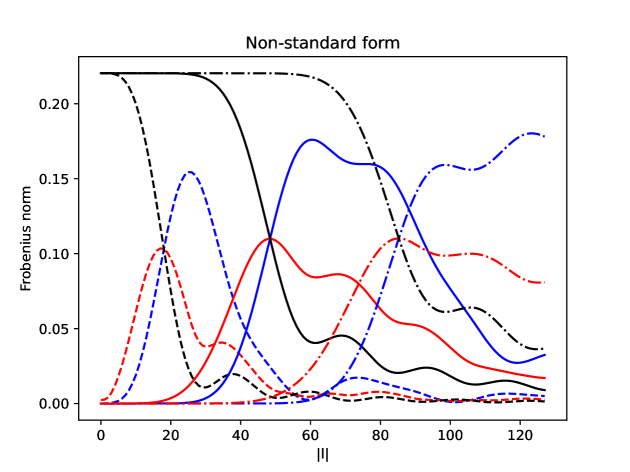
Figure 1. Sparsity of the non-standard form at scale $n=7$ corresponding to the time step $t=0.0001$. Here $\left\|\alpha_{l}\right\|$ is blue, $\left\|\beta_{l}\right\|$ is red, $\left\|\sigma_{l}\right\|$ is black. Solid line corresponds to $\mathfrak{k}=6$, dashed to $\mathfrak{k}=2$ and dash-dot to $\mathfrak{k}=11$. For $\mathfrak{k}=2$ we have the values on the diagonal $\left\|\alpha_{0}\right\|=\text{8.0e-05},\left\|\beta_{0}\right\|=\text{2.4e-03},$ and in the corner $\left\|\alpha_{2^{n}-1}\right\|=\text{5.0e-03},\left\|\beta_{2^{n}-1}\right\|=\text{2.6e-03}.$ For $\mathfrak{k}=6$ we have the values on the diagonal $\left\|\alpha_{0}\right\|=\text{3.2e-13},\left\|\beta_{0}\right\|=\text{3.9e-08},$ and in the corner $\left\|\alpha_{2^{n}-1}\right\|=\text{3.2e-02},\left\|\beta_{2^{n}-1}\right\|=\text{1.7e-02}.$ For $\mathfrak{k}=11$ we have the values on the diagonal $\left\|\alpha_{0}\right\|=\text{2.7e-18},\left\|\beta_{0}\right\|=\text{4.0e-15},$ and in the corner $\left\|\alpha_{2^{n}-1}\right\|=\text{1.8e-01},\left\|\beta_{2^{n}-1}\right\|=\text{8.1e-02}.$

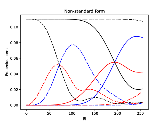
Figure 2. Sparsity of the non-standard form at scale $n=8$ corresponding to the time step $t=0.0001$. Here $\left\|\alpha_{l}\right\|$ is blue, $\left\|\beta_{l}\right\|$ is red, $\left\|\sigma_{l}\right\|$ is black. Solid line corresponds to $\mathfrak{k}=6$, dashed to $\mathfrak{k}=2$ and dash-dot to $\mathfrak{k}=11$. For $\mathfrak{k}=2$ we have the values on the diagonal $\left\|\alpha_{0}\right\|=\text{2.5e-06},\left\|\beta_{0}\right\|=\text{3.0e-04},$ and in the corner $\left\|\alpha_{2^{n}-1}\right\|=\text{3.2e-03},\left\|\beta_{2^{n}-1}\right\|=\text{3.2e-03}.$ For $\mathfrak{k}=6$ we have the values on the diagonal $\left\|\alpha_{0}\right\|=\text{3.9e-17},\left\|\beta_{0}\right\|=\text{3.1e-10},$ and in the corner $\left\|\alpha_{2^{n}-1}\right\|=\text{8.6e-02},\left\|\beta_{2^{n}-1}\right\|=\text{4.2e-02}.$ For $\mathfrak{k}=11$ we have the values on the diagonal $\left\|\alpha_{0}\right\|=\text{5.2e-19},\left\|\beta_{0}\right\|=\text{3.5e-18},$ and in the corner $\left\|\alpha_{2^{n}-1}\right\|=\text{2.9e-03},\left\|\beta_{2^{n}-1}\right\|=\text{1.8e-02}.$

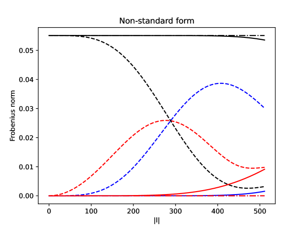
Figure 3. Sparsity of the non-standard form at scale $n=9$ corresponding to the time step $t=0.0001$. Here $\left\|\alpha_{l}\right\|$ is blue, $\left\|\beta_{l}\right\|$ is red, $\left\|\sigma_{l}\right\|$ is black. Solid line corresponds to $\mathfrak{k}=6$, dashed to $\mathfrak{k}=2$ and dash-dot to $\mathfrak{k}=11$. For $\mathfrak{k}=2$ we have the values on the diagonal $\left\|\alpha_{0}\right\|=\text{7.8e-08},\left\|\beta_{0}\right\|=\text{3.8e-05},$ and in the corner $\left\|\alpha_{2^{n}-1}\right\|=\text{3.0e-02},\left\|\beta_{2^{n}-1}\right\|=\text{9.8e-03}.$ For $\mathfrak{k}=6$ we have the values on the diagonal $\left\|\alpha_{0}\right\|=\text{5.3e-19},\left\|\beta_{0}\right\|=\text{2.4e-12},$ and in the corner $\left\|\alpha_{2^{n}-1}\right\|=\text{1.6e-03},\left\|\beta_{2^{n}-1}\right\|=\text{9.1e-03}.$ For $\mathfrak{k}=11$ we have the values on the diagonal $\left\|\alpha_{0}\right\|=\text{3.2e-19},\left\|\beta_{0}\right\|=\text{1.5e-18},$ and in the corner $\left\|\alpha_{2^{n}-1}\right\|=\text{6.8e-09},\left\|\beta_{2^{n}-1}\right\|=\text{1.9e-05}.$

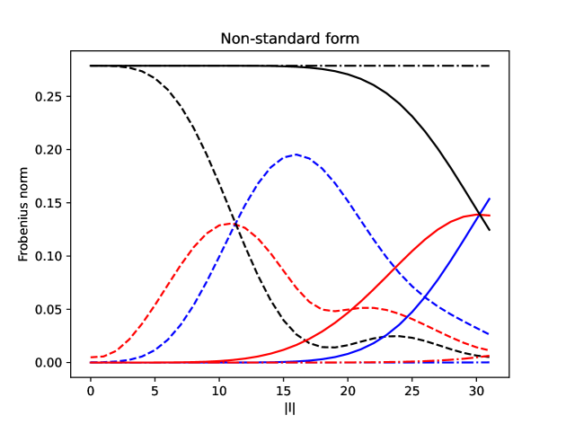
Figure 4. Sparsity of the non-standard form at scale $n=5$ corresponding to the time step $t=0.001$. Here $\left\|\alpha_{l}\right\|$ is blue, $\left\|\beta_{l}\right\|$ is red, $\left\|\sigma_{l}\right\|$ is black. Solid line corresponds to $\mathfrak{k}=6$, dashed to $\mathfrak{k}=2$ and dash-dot to $\mathfrak{k}=11$. For $\mathfrak{k}=2$ we have the values on the diagonal $\left\|\alpha_{0}\right\|=\text{2.6e-04},\left\|\beta_{0}\right\|=\text{4.9e-03},$ and in the corner $\left\|\alpha_{2^{n}-1}\right\|=\text{2.6e-02},\left\|\beta_{2^{n}-1}\right\|=\text{1.1e-02}.$ For $\mathfrak{k}=6$ we have the values on the diagonal $\left\|\alpha_{0}\right\|=\text{6.8e-12},\left\|\beta_{0}\right\|=\text{2.0e-07},$ and in the corner $\left\|\alpha_{2^{n}-1}\right\|=\text{1.5e-01},\left\|\beta_{2^{n}-1}\right\|=\text{1.4e-01}.$ For $\mathfrak{k}=11$ we have the values on the diagonal $\left\|\alpha_{0}\right\|=\text{2.4e-18},\left\|\beta_{0}\right\|=\text{8.5e-14},$ and in the corner $\left\|\alpha_{2^{n}-1}\right\|=\text{1.5e-04},\left\|\beta_{2^{n}-1}\right\|=\text{6.4e-03}.$

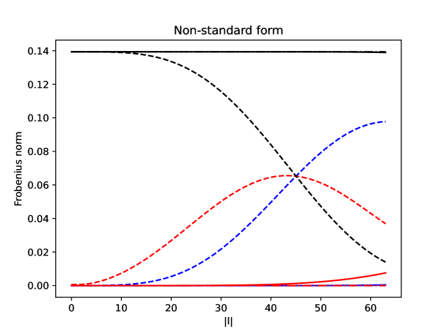
Figure 5. Sparsity of the non-standard form at scale $n=6$ corresponding to the time step $t=0.001$. Here $\left\|\alpha_{l}\right\|$ is blue, $\left\|\beta_{l}\right\|$ is red, $\left\|\sigma_{l}\right\|$ is black. Solid line corresponds to $\mathfrak{k}=6$, dashed to $\mathfrak{k}=2$ and dash-dot to $\mathfrak{k}=11$. For $\mathfrak{k}=2$ we have the values on the diagonal $\left\|\alpha_{0}\right\|=\text{8.1e-06},\left\|\beta_{0}\right\|=\text{6.1e-04},$ and in the corner $\left\|\alpha_{2^{n}-1}\right\|=\text{9.8e-02},\left\|\beta_{2^{n}-1}\right\|=\text{3.7e-02}.$ For $\mathfrak{k}=6$ we have the values on the diagonal $\left\|\alpha_{0}\right\|=\text{8.3e-16},\left\|\beta_{0}\right\|=\text{1.6e-09},$ and in the corner $\left\|\alpha_{2^{n}-1}\right\|=\text{4.1e-04},\left\|\beta_{2^{n}-1}\right\|=\text{7.5e-03}.$ For $\mathfrak{k}=11$ we have the values on the diagonal $\left\|\alpha_{0}\right\|=\text{6.3e-19},\left\|\beta_{0}\right\|=\text{1.1e-17},$ and in the corner $\left\|\alpha_{2^{n}-1}\right\|=\text{1.4e-10},\left\|\beta_{2^{n}-1}\right\|=\text{4.3e-06}.$

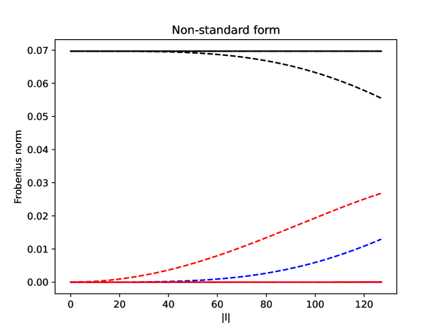
Figure 6. Sparsity of the non-standard form at scale $n=7$ corresponding to the time step $t=0.001$. Here $\left\|\alpha_{l}\right\|$ is blue, $\left\|\beta_{l}\right\|$ is red, $\left\|\sigma_{l}\right\|$ is black. Solid line corresponds to $\mathfrak{k}=6$, dashed to $\mathfrak{k}=2$ and dash-dot to $\mathfrak{k}=11$. For $\mathfrak{k}=2$ we have the values on the diagonal $\left\|\alpha_{0}\right\|=\text{2.5e-07},\left\|\beta_{0}\right\|=\text{7.7e-05},$ and in the corner $\left\|\alpha_{2^{n}-1}\right\|=\text{1.3e-02},\left\|\beta_{2^{n}-1}\right\|=\text{2.7e-02}.$ For $\mathfrak{k}=6$ we have the values on the diagonal $\left\|\alpha_{0}\right\|=\text{4.2e-19},\left\|\beta_{0}\right\|=\text{1.2e-11},$ and in the corner $\left\|\alpha_{2^{n}-1}\right\|=\text{1.1e-07},\left\|\beta_{2^{n}-1}\right\|=\text{8.8e-05}.$ For $\mathfrak{k}=11$ we have the values on the diagonal $\left\|\alpha_{0}\right\|=\text{2.0e-19},\left\|\beta_{0}\right\|=\text{1.8e-18},$ and in the corner $\left\|\alpha_{2^{n}-1}\right\|=\text{3.0e-17},\left\|\beta_{2^{n}-1}\right\|=\text{1.4e-09}.$

Finally, we turn our attention to the sparsity of matrices (4.3)-(4.5) associated with the nonstandard form (2.14) by means of (2.13), (2.15). One can calculate matrices $\sigma_{l}^{n+1},l=1-2^{n+1},\ldots,2^{n+1}-1,$ using the expansion (4.18) and then find matrices $\alpha_{l}^{n},\beta_{l}^{n},\gamma_{l}^{n}$ with $l=1-2^{n},\ldots,2^{n}-1$ exploiting (3.7). The Frobenius norm

$$\left\|\alpha\right\|=\left(\sum_{p,j=0}^{\mathfrak{k}-1}\left|\left[\alpha\right]_{pj}\right|^{2}\right)^{1/2}$$ (4.22)

is used for a matrix $\alpha$ of $\mathfrak{k}\times\mathfrak{k}$-size. Figures 1 - 6 demonstrate the tendency of considerable non-zero values $\left\|\alpha_{l}^{n}\right\|,\left\|\beta_{l}^{n}\right\|$ to stay away from the main diagonal $l=0$. It is in contrast with the fact that the non-standard form matrices of the heat equation are narrow diagonal bounded as we mentioned in Subsection 3.2. Intuitively, this difference can be explained as follows. The heat defuses with time, that is, it transports away from the initial local perturbation point with some smearing. Waves described by the Schrödinger equation (1.3) disperse. Such a wave moves away from the initial local perturbation point forming high frequency ripples that are captured by multiresolution analysis.

Alternatively, the values on the diagonal and away could be roughly estimated as follows. Due to the vanishing moment property (2.7), $\widehat{\psi}_{j}(\zeta)$ has a root at zero of order $\mathfrak{k}+j$. It results in the fact, that the corresponding expansions, similar to (4.18), for the matrix elements $\left[\alpha_{l}^{n}\right]_{pj}$ and $\left[\beta_{l}^{n}\right]_{pj}$ start with integrals $J_{2\mathfrak{k}+p+j}$ and $J_{\mathfrak{k}+p+j}$, respectively. These integrals constitute the leading terms, due to their fast convergence to zero. Moreover, the corner elements $\left[\alpha_{l}^{n}\right]_{00}$ and $\left[\beta_{l}^{n}\right]_{00}$ are dominant for the same reason. Therefore, $\left\|\alpha_{l}^{n}\right\|\sim|J_{2\mathfrak{k}}(l)|$ and $\left\|\beta_{l}^{n}\right\|\sim|J_{\mathfrak{k}}(l)|.$

For $l=0$ from (4.20) one obtains

$$J_{2k}(0)=\frac{e^{i\pi(2k-1)/4}}{2\sqrt{\pi a}(2a)^{k}(2k+2)!!(2k+1)},\quad J_{2k+1}(0)=0.$$ (4.23)

In the case of $|l|\gg 1$, we can admit the following approximation

$$J_{m+1}(l)\approx\frac{il}{2a(m+3)}J_{m}(l)$$

and so

$$J_{m}(l)\approx\left(\frac{il}{2a}\right)^{m}\frac{\exp\left(\frac{il^{2}}{4a}-\frac{i\pi}{4}\right)}{2\sqrt{\pi a}(m+2)!}$$ (4.24)

which leads to

$$\left\|\alpha_{l}^{n}\right\|\lesssim\frac{1}{2\sqrt{\pi a}(2\mathfrak{k}+2)!}\left(\frac{l}{2a}\right)^{2\mathfrak{k}},\quad|l|\gg 1$$

Meanwhile, $\left\|\alpha_{0}^{n}\right\|\sim|J_{2\mathfrak{k}}(0)|,$ where the integral is calculated in (4.23). Thus

$$\left\|\alpha_{l}^{n}\right\|\lesssim\frac{1}{2\sqrt{\pi a}(2a)^{\mathfrak{k}}(2\mathfrak{k}+2)!!(2\mathfrak{k}+1)}+\frac{1}{2\sqrt{\pi a}(2\mathfrak{k}+2)!}\left(\frac{l}{2a}\right)^{2\mathfrak{k}}$$

Similarly,

$$\left\|\beta_{l}^{n}\right\|=\left\|\gamma_{l}^{n}\right\|\lesssim\frac{1}{2\sqrt{\pi a}(2a)^{\mathfrak{k}/2}(\mathfrak{k}+2)!!(\mathfrak{k}+1)}+\frac{1}{2\sqrt{\pi a}(\mathfrak{k}+2)!}\left(\frac{l}{2a}\right)^{\mathfrak{k}},\quad\text{provided $\mathfrak{k}$ is even}$$

and

$$\left\|\beta_{l}^{n}\right\|=\left\|\gamma_{l}^{n}\right\|\lesssim\frac{1}{2\sqrt{\pi a}(2a)^{(\mathfrak{k}+1)/2}(\mathfrak{k}+3)!!(\mathfrak{k}+2)}+\frac{1}{2\sqrt{\pi a}(\mathfrak{k}+2)!}\left(\frac{l}{2a}\right)^{\mathfrak{k}},\quad\text{provided $\mathfrak{k}$ is odd.}$$

Note that the expansions for matrices $\alpha_{l}^{n}$, $\beta_{l}^{n}$ with respect to the power integrals contain cross correlation coefficients depending on the MRA order $\mathfrak{k}$. Therefore, the implicit constants staying in the obtained inequalities for $\left\|\alpha_{l}^{n}\right\|,\left\|\beta_{l}^{n}\right\|$ depend on $\mathfrak{k}$ as well. In other words, these inequalities provide only with a qualitative behaviour of the norms. For instance, one can compare

$$|J_{2\mathfrak{k}}(0)|=\left\{\begin{aligned} \text{8.6e-05, }\quad\mathfrak{k}=2\\ \text{2.1e-11, }\quad\mathfrak{k}=6\\ \text{1.0e-20,}\quad\mathfrak{k}=11\end{aligned}\right.$$

for $n=7$ and $t=0.0001$ with the values $\left\|\alpha_{0}^{n}\right\|$ given in the caption of Figure 1.

4.2. Interpolating scaling functions

Similarly to the case of Legendre scaling functions, we introduce functions $\Psi_{j}(-i\zeta)=\widehat{\varphi}_{j}(\zeta),$ so that

$$\Psi_{j}(x)=\sqrt{w_{j}}\sum_{m=0}^{\mathfrak{k}-1}\phi_{m}(x_{j})\Phi_{m}(x),\quad x\in(0,1),\quad j=0,\ldots,\mathfrak{k}-1,$$

where $\phi_{m}$ are the Legendre scaling functions. Here $x_{0},\ldots,x_{\mathfrak{k}-1}$ denote the roots of $P_{\mathfrak{k}}(2x-1)$. We are interested in the following combination

$$\Psi_{j}(-x)\Psi_{p}(x)=\sqrt{w_{j}w_{p}}\sum_{j^{\prime},p^{\prime}=0}^{\mathfrak{k}-1}\phi_{j^{\prime}}(x_{j})\phi_{p^{\prime}}(x_{p})\Phi_{j^{\prime}}(-x)\Phi_{p^{\prime}}(x).$$

Thus it can be presented as the series

$$\Psi_{j}(-x)\Psi_{p}(x)=\sum_{k=0}^{\infty}\frac{D_{jp}^{k}x^{k}}{(k+2)!},$$

where

$$D_{jp}^{k}=\sqrt{w_{j}w_{p}}\sum_{\begin{subarray}{c}0\leqslant j^{\prime},p^{\prime}\leqslant\mathfrak{k}-1\\ j^{\prime}+p^{\prime}\leqslant k\end{subarray}}\phi_{j^{\prime}}(x_{j})\phi_{p^{\prime}}(x_{p})C_{j^{\prime}p^{\prime}}^{k-j^{\prime}-p^{\prime}},\quad j,p=0,\ldots,\mathfrak{k}-1.$$

Note that this double sum can be restricted to $k-j^{\prime}-p^{\prime}$ being even non-negative. Thus our main operator in the interpolating basis has the following expansion

$$\left[\sigma_{l}^{n}\right]_{pj}(a)=\sum_{k=0}^{\infty}D_{jp}^{k}J_{k}(l,a),$$ (4.25)

where as above $a=tN^{2}=t4^{n}$.

Calculating matrices $\alpha_{l}^{n},\beta_{l}^{n},\gamma_{l}^{n}$ from $\sigma_{l}^{n+1}$ by (3.7) and then evaluating the norms $\left\|\alpha_{l}^{n}\right\|,\left\|\beta_{l}^{n}\right\|$ and $\left\|\gamma_{l}^{n}\right\|,$ one arrives to qualitatively the same results as above, and so we do not illustrate them on separate figures.

4.3. Haar multiresolution analysis

The above conclusions simplify significantly in the case $\mathfrak{k}=1$. By (4.6), (3.3) we have

$$\left[\sigma_{l}^{n}\right]_{00}=\int_{\Gamma}F(\zeta)d\zeta,\quad F(\zeta)=\frac{1-\cos\zeta}{\pi\zeta^{2}}\exp\left(i\zeta l-itN^{2}\zeta^{2}\right).$$

Let us first justify (4.1), so we regard $\zeta$ lying in the band $|\operatorname{Im}\zeta|\leqslant H$ and satisfying $\operatorname{Re}\zeta\cdot\operatorname{Im}\zeta\leqslant 0$, then

$$\left|F(\zeta)\right|\leqslant\frac{2}{\pi}e^{H(|l|+1)}\leqslant\frac{2}{\pi}e^{HN}.$$

In order to maintain accuracy $\varepsilon$, while discretizing the integral in such domain, the right hand of this bound should not be bigger than $\varepsilon/\varepsilon_{\text{mach}}$. Thus we obtained (4.1).

Now we have only even power integrals in the expansion (4.18),

$$\left[\sigma_{l}^{n}\right]_{00}=2\sum_{k=0}^{\infty}J_{2k}(l,a),$$ (4.26)

since $C_{00}^{k}=1+(-1)^{k}$ by (4.17), that of course can be checked directly by expanding $\cos\zeta$ about zero. The convergence rate of this series was analysed in Subsection 4.1.

Finally, let us have a closer look at the dependence of $\left[\sigma_{l}^{n}\right]_{00}$ on the distance $|l|$ to the diagonal. In the case of $l=0$, one can calculate the sum of the series by means of special functions as

$$\left[\sigma_{0}^{n}\right]_{00}=-i\sqrt{\frac{2}{\pi}}F_{1}\left(\frac{e^{\frac{i\pi}{4}}}{\sqrt{2a}}\right),$$ (4.27)

where

$$F_{1}(x)=\sum_{k=0}^{\infty}\frac{x^{2k+1}}{(2k+1)(2k+2)!!}=\frac{1-e^{x^{2}/2}}{x}-i\sqrt{\frac{\pi}{2}}\operatorname{erf}\left(\frac{ix}{\sqrt{2}}\right),$$

using (4.23). The series $F_{1}\left(\frac{e^{\frac{i\pi}{4}}}{\sqrt{2a}}\right)$ is very useful in practice for the precision control, since its real and imaginary parts are alternating series with monotonically decreasing coefficients.

In the case of $|l|\gg 1$, we have (4.24) which leads to

$$\left[\sigma_{l}^{n}\right]_{00}\approx\frac{1}{\sqrt{\pi a}}\left(\frac{2a}{l}\right)^{2}\left(1-\cos\frac{l}{2a}\right)\exp\left(\frac{il^{2}}{4a}-\frac{i\pi}{4}\right).$$ (4.28)

Here the term in front of the exponent changes slowly with $l$, whereas the exponent itself oscillates very fast. This formula describes the operator matrix with a very high precision for any $l\neq 0$. In fact the limit of this expression as $l/{2a}\to 0$ is identical to $\left[\sigma_{0}^{n}\right]_{00}$ evaluated by (4.27) with the first order approximation $F_{1}(x)\approx x/2$. Moreover, (4.27) and (4.28) give us an idea of how many terms are important in Expansion (4.26) for a given precision. The same series cut is reliable in practise for evaluation of the general expansion (4.18).

5. Introduction into exponential integrators

It is known that a fundamental solution of the general linear equation

$$\partial_{t}u=Au+Bu$$ (5.1)

forms a two-parameter family of operators $\mathcal{T}(t_{2},t_{1})$ called propagator. It means that for any solution $u=u(t)$ of (5.1) and time moments $t_{1},t_{2}$ we have $u(t_{2})=\mathcal{T}(t_{2},t_{1})u(t_{1}).$ This section serves as a brief reminder of how this propagator can be approximated by the exponential operators $e^{At},e^{Bt},$ providing us with effective numerical schemes for (5.1). Up to the imaginary unit, $A$ and $B$ will stand for kinetic and potential operators below, as in Equation (1.1), for example.

5.1. Time independent potential

Let $A,B$ be constant. Then the propagator $\mathcal{T}$ reduces to the one-parameter family $\mathcal{T}(t_{2},t_{1})=\mathcal{T}(t_{2}-t_{1})$ with $\mathcal{T}(t)=e^{(A+B)t}$ called a semigroup. Since in general operators $A$ and $B$ do not commute, one cannot substitute this exponent with the multiplication of semigroups associated with $A$ and $B$ each. On the contrary, such substitution is valid for small $t$, namely,

$$e^{At+Bt}=e^{At}e^{Bt}+\mathcal{O}\left(t^{2}\right).$$ (5.2)

A subsequent application of the multiplication $e^{At}e^{Bt}$ to a given initial data $u(0)$ would provide us with the solution at a given final time moment with first order $\mathcal{O}\left(t\right)$ of accuracy. A more accurate result one can get with the symmetric symplectic scheme (1.4). General higher order factorizations of this type were systematically investigated in [34, 42]. For any given positive integer $n$ one can decompose the semigroup $\mathcal{T}(t)$ as

$$e^{At+Bt}=e^{At_{1}}e^{Bt_{2}}e^{At_{3}}e^{Bt_{4}}\ldots e^{At_{M}}+\mathcal{O}\left(t^{n+1}\right)$$ (5.3)

with some appropriately chosen parameters $t_{1},\ldots,t_{M}$. It allows to set bigger time steps and accelerate computations. However, it turns out that $M$ increases with $n$ exponentially, and so in practice the integrator order $n$ is chosen no bigger than $8$, since too many exponents in the decomposition formula can on the opposite slow down the calculations. Moreover, the time parameters $t_{1},\ldots,t_{M}$ are not unique. Below we try to choose those ones that lead to exponents $\exp\left(it_{j}\partial_{x}^{2}\right)$ in the decomposition (5.3) with overall biggest possible absolute values $\left|t_{j}\right|$ to incorporate the multiresolution sparsity at most.

So far we have not employed the fact that $A$ stands for the kinetic and $B$ for the potential energy operators. An advantage of this particular choice was taken in [14, 15, 36], where several fourth order schemes were introduced allowing minimal amount of exponents in the decomposition (5.3). Among them we extensively use the following

$$e^{At+Bt}=\exp\left(\frac{t}{6}B\right)\exp\left(\frac{t}{2}A\right)\exp\left(\frac{2t}{3}\widetilde{B}\right)\exp\left(\frac{t}{2}A\right)\exp\left(\frac{t}{6}B\right)+\mathcal{O}\left(t^{5}\right),$$ (5.4)

where

$$\widetilde{B}=\widetilde{B}(t)=B+\frac{t^{2}}{48}[B,[A,B]].$$

This double commutator is proportional to the squared gradient of the potential $(\partial_{x}V)^{2},$ which makes $\widetilde{B}$ a potential operator when $B=-iV$. Indeed,

$$\widetilde{B}=-i\widetilde{V},\quad\widetilde{V}=\left\{\begin{aligned} &V-\frac{t^{2}}{24}(\partial_{x}V)^{2},\quad A=i\partial_{x}^{2},\quad B=-iV\\ &V-\frac{t^{2}}{48}(\partial_{x}V)^{2},\quad A=\frac{i}{2}\partial_{x}^{2},\quad B=-iV\end{aligned}\right.,$$

where we regarded two of the most used normalisations for the kinetic energy operator. The fourth order scheme (5.4) requires only two applications of the free-particle semigroup operator. On the contrary it demands to know the gradient of the potential. For comparison we mention an alternative scheme from [15] reading

$$e^{At+Bt}=\exp\left(\frac{t}{8}\widetilde{B}\right)\exp\left(\frac{t}{3}A\right)\exp\left(\frac{3t}{8}B\right)\exp\left(\frac{t}{3}A\right)\exp\left(\frac{3t}{8}B\right)\exp\left(\frac{t}{3}A\right)\exp\left(\frac{t}{8}\widetilde{B}\right)+\mathcal{O}\left(t^{5}\right),$$ (5.5)

where $\widetilde{B}$ is the same. Apart from the fact that the free-particle operator $\exp\left(\frac{t}{3}A\right)$ appears here 3 times, the factor $1/3$ in front of $tA$ makes its multiresolution less sparse comparing to $\exp\left(\frac{t}{2}A\right)$ standing in (5.4). Scheme (5.5) could potentially be of use only together with (5.4) for precision control. The operator splitting (5.4) is far superior to any other existing fourth order symplectic algorithm, to our knowledge.

These algorithms can be recursively extended to higher order schemes [15]. Denoting by $\mathcal{T}$ the evolution operator $\mathcal{T}(t)=e^{At+Bt}$ and by $\mathcal{T}^{(n)}$ its $n$-th order approximation, that is $\mathcal{T}(t)=\mathcal{T}^{(n)}(t)+\mathcal{O}\left(t^{n+1}\right),$ we can express an $n+2$ order scheme as

$$\mathcal{T}^{(n+2)}(t)=\mathcal{T}^{(n)}(t_{n})\mathcal{T}^{(n)}(-s_{n}t_{n})\mathcal{T}^{(n)}(t_{n}),\quad t_{n}=\frac{t}{2-s_{n}},\quad s_{n}=2^{1/(n+1)}.$$ (5.6)

A proof can be found in [42]. We make a couple of remarks concerning this recursive formula. Firstly, $\mathcal{T}(-t)=\mathcal{T}^{-1}(t)$ that is in connection to the Schrödinger equation coincides with the adjoint $\mathcal{T}^{*}(t)$. Secondly, $s_{n}t_{n}>t_{n}>t$, which provides us with a little advantage of exploiting (5.6), since the precision and sparsity of the free particle propagator multiresolution is increasing together with the time step. Although there is an obvious drawback behind (5.6), as the amount of work is increasing three times per time step whenever one goes for a higher order scheme. As a working example of a sixth order scheme, we iterate $\mathcal{T}^{(4)}$ given by (5.4) using (5.6) to get

$$\mathcal{T}^{(6)}(t)= \exp\left(\frac{t_{4}}{6}B\right)\exp\left(\frac{t_{4}}{2}A\right)\exp\left(\frac{2t_{4}}{3}\widetilde{B}(t_{4})\right)\exp\left(\frac{t_{4}}{2}A\right)\exp\left(\frac{(1-s_{4})t_{4}}{6}B\right)$$

$$\exp\left(-\frac{s_{4}t_{4}}{2}A\right)\exp\left(-\frac{2s_{4}t_{4}}{3}\widetilde{B}(s_{4}t_{4})\right)\exp\left(-\frac{s_{4}t_{4}}{2}A\right)$$

$$\exp\left(\frac{(1-s_{4})t_{4}}{6}B\right)\exp\left(\frac{t_{4}}{2}A\right)\exp\left(\frac{2t_{4}}{3}\widetilde{B}(t_{4})\right)\exp\left(\frac{t_{4}}{2}A\right)\exp\left(\frac{t_{4}}{6}B\right).$$ (5.7)

Here the last 6 operators are the first 6 operators following in reverse, so that the whole operator $\mathcal{T}^{(6)}(t)$ is symmetric. Note that this scheme demands 6 applications of kinetic energy exponent per time step. If we continue the recursive procedure (5.6) we will arrive to an eighth order scheme demanding 18 applications, correspondingly. It is still a reasonable amount. However, at this level there is a slightly better alternative derived by Yoshida [42] that we describe next. It is clear from the iterative procedure (5.6) that an even order symmetric integrator can have the form

$$\mathcal{T}^{(n)}(t)=\mathcal{T}^{(2)}(w_{m}t)\ldots\mathcal{T}^{(2)}(w_{0}t)\ldots\mathcal{T}^{(2)}(w_{m}t)$$

with $2m+1$ second order integrators $\mathcal{T}^{(2)}(t)$ defined by the splitting (1.4) and some weights $w_{0},w_{1},\ldots,w_{m}$. Number $m$ and these weights depend on the order $n$. However, a direct implementation of (5.6) does not necessarily give the most optimal representation. It turns out that $m$ can be diminished down to $m=3$ for the order $n=6$ and to $m=7$ for the order $n=8$. The weights are not unique, we choose those providing us with the biggest value $\min\limits_{j=0,\ldots,m}|w_{j}|,$ namely, set A from Table 1 and set C from Table 2 in [42]. They are repeated below for convenience.

1. $$w_{0}=1.315186320683906,\quad w_{1}=-1.17767998417887,$$

   $$w_{2}=0.235573213359357,\quad w_{3}=0.784513610477560.$$

2. $$w_{0}=1.65899088454396,\quad w_{1}=0.311790812418427,$$

   $$w_{2}=-1.55946803821447,\quad w_{3}=-1.67896928259640,$$

   $$w_{4}=1.66335809963315,\quad w_{5}=-1.06458714789183,$$

   $$w_{6}=1.36934946416871,\quad w_{7}=0.629030650210433.$$

Thus both 6th and 8th order Yoshida integrators can be combined together in the product

$$\mathcal{T}^{(n)}(t)=\exp(c_{1}tB)\exp(d_{1}tA)\exp(c_{2}tB)\cdot\ldots\cdot\exp(d_{2m+1}tA)\exp(c_{2m+2}tB)$$ (5.8)

where $t$ is the time step and $c_{i}$, $d_{i}$ are constants given by

$$c_{1}=c_{2m+2}=\frac{w_{m}}{2},\quad c_{2}=c_{2m+1}=\frac{w_{m}+w_{m-1}}{2},\quad\ldots,\quad c_{m+1}=c_{m+2}=\frac{w_{1}+w_{0}}{2}$$

and

$$d_{1}=d_{2m+1}=w_{m},\quad d_{2}=d_{2m}=w_{m-1},\quad\ldots,\quad d_{m}=d_{m+2}=w_{1},\quad d_{m+1}=w_{0}.$$

One can notice that the integrator is symmetric. Moreover, it is quite general, one does not need to know the potential gradient $\partial_{x}V(x)$. The 8th order scheme demands 15 kinetic exponent applications, less than 18 corresponding to the twice iterated (5.4) by (5.6). The weights associated with the latter lie in the interval $[0.65,0.84]$ in absolute value, as one can easily deduce from (5.4), (5.6). Thus in the case of stationary potential $V(x)$ one may anticipate the best performance for

1. Scheme (5.4),

2. Scheme (5.1),

3. Scheme (5.8).

The difference between Scheme (5.1) and Scheme (5.8) is mild, though in [15] it is claimed that (5.1) outperforms slightly (5.8) at least for the scattering experiment regarded there.

5.2. Time dependent potential

Now let $B=B(t)$, the propagator $\mathcal{T}=\mathcal{T}(t+\tau,t)$ can still be approximated at a small time step $\tau=\Delta t$ by exponential operators. An $n$-th order integrator propagating solutions of (5.1) through the interval $[t,t+\tau]$ is denoted by $\mathcal{T}^{(n)}(t+\tau,t)$, meaning $\mathcal{T}(t+\tau,t)=\mathcal{T}^{(n)}(t+\tau,t)+\mathcal{O}\left(\tau^{n+1}\right).$ Using Suzuki’s formal approach [35] we extend the schemes from the previous subsection to the current situation. Let $\mathcal{D}$ be the forward time derivative operator, called also the super-operator in [35], that is a time derivative acting on functions standing on the left, namely,

$$F(t)e^{\tau\mathcal{D}}G(t)=F(t+\tau)G(t)$$ (5.9)

for any time-dependent functions $F(t)$ and $G(t)$. In particular, $e^{\tau\mathcal{D}}G(t)=G(t).$ With the help of this super-operator the propagator is reduced to the exponential representation

$$\mathcal{T}(t+\tau,t)=\exp\left(\tau(A+B(t)+\mathcal{D})\right).$$ (5.10)

Combining $A$, $\mathcal{D}$ together and approximating this exponent exactly as was done in the previous subsection with $A+\mathcal{D}$ standing now in place of $A$ we can extend all the above schemes. Note that $A$ does not depend on time, so $A$ and $\mathcal{D}$ commute. Therefore, $\exp\left(\tau(A+\mathcal{D})\right)=\exp\left(\tau A)\right)\exp\left(\tau\mathcal{D}\right).$ Thus approximating the exponent in (5.10) by the second order scheme (1.4) one deduces

$$\mathcal{T}(t+\tau,t)=\exp\left(\frac{\tau}{2}B(t)\right)\exp\left(\tau(A+\mathcal{D})\right)\exp\left(\frac{\tau}{2}B(t)\right)+\mathcal{O}\left(t^{3}\right)$$

which together with the super-operator property (5.9) leads to the following simple second order splitting

$$\mathcal{T}^{(2)}(t+\tau,t)=\exp\left(\frac{\tau}{2}B(t+\tau)\right)\exp\left(\tau A\right)\exp\left(\frac{\tau}{2}B(t)\right).$$ (5.11)

In the same manner we extend both 6th and 8th order Yoshida integrators to

$$\mathcal{T}^{(n)}(t+\tau,t)=\exp(c_{1}\tau B(t+b_{1}\tau))\exp(d_{1}\tau A)\exp(c_{2}\tau B(t+b_{2}\tau))\\ \cdot\ldots\cdot\exp(d_{2m+1}\tau A)\exp(c_{2m+2}\tau B(t+b_{2m+2}\tau)),$$ (5.12)

where $b_{k}$ are constants given by

$$b_{k}=\sum_{j=k}^{2m+1}d_{j}=1-\sum_{j=1}^{k-1}d_{j},$$

in particular, $b_{1}=1$ and $b_{2m+2}=0$.

In the case of time dependent potential there is an analogue of (5.4) in [16] reading

$$\mathcal{T}^{(4)}(t+\tau,t)=\exp\left(\frac{\tau}{6}B(t+\tau)\right)\exp\left(\frac{\tau}{2}A\right)\exp\left(\frac{2{\tau}}{3}\widetilde{B}\left(t+\frac{\tau}{2},\tau\right)\right)\exp\left(\frac{\tau}{2}A\right)\exp\left(\frac{\tau}{6}B(t)\right),$$ (5.13)

where the modified potential given at the middle step time moment is defined as

$$\widetilde{B}(t,\tau)=B(t)+\frac{\tau^{2}}{48}\left[B(t),\left[A,B(t)\right]\right].$$ (5.14)

This follows from (5.10), (5.4), (5.9) and the identity $[B(t),[\mathcal{D},B(t)]]=0.$ The latter can be checked directly

$$F(t)[B(t),[\mathcal{D},B(t)]]=2F(t)B(t)\mathcal{D}B(t)-F(t)B^{2}(t)\mathcal{D}-F(t)\mathcal{D}B^{2}(t)=0$$

on any smooth test operator $F(t)$. Scheme (5.13) is very useful, since the commutator in (5.14) turns out to be proportional to $\partial_{x}V(x,t)$ for the Schrödinger equation, compare also with the same scheme obtained recently for the Dirac equation [41]. Similarly, the sixth order integrator (5.1) turns into

$$\mathcal{T}^{(6)}(t+\tau,t)=\exp\left(\frac{\tau_{4}}{6}B(t+(2-s_{4})\tau_{4})\right)\exp\left(\frac{\tau_{4}}{2}A\right)\exp\left(\frac{2\tau_{4}}{3}\widetilde{B}\left(t+\left(\frac{3}{2}-s_{4}\right)\tau_{4},\tau_{4}\right)\right)\\ \cdot\exp\left(\frac{\tau_{4}}{2}A\right)\exp\left(\frac{(1-s_{4})\tau_{4}}{6}B(t+\left(1-s_{4}\right)\tau_{4})\right)\exp\left(-\frac{s_{4}\tau_{4}}{2}A\right)\\ \cdot\exp\left(-\frac{2s_{4}\tau_{4}}{3}\widetilde{B}\left(t+\left(1-\frac{s_{4}}{2}\right)\tau_{4},s_{4}\tau_{4}\right)\right)\exp\left(-\frac{s_{4}\tau_{4}}{2}A\right)\exp\left(\frac{(1-s_{4})\tau_{4}}{6}B(t+\tau_{4})\right)\\ \cdot\exp\left(\frac{\tau_{4}}{2}A\right)\exp\left(\frac{2\tau_{4}}{3}\widetilde{B}\left(t+\frac{\tau_{4}}{2},\tau_{4}\right)\right)\exp\left(\frac{\tau_{4}}{2}A\right)\exp\left(\frac{\tau_{4}}{6}B(t)\right).$$ (5.15)

Note that we first extended the time-independent potential scheme (5.4) to (5.1) via recursion (5.6), afterwards we applied the Suzuki decomposition method (5.10) to deduce (5.15) from (5.1). Integrator (5.13) can also be directly extended to higher order schemes by the general Suzuki’s recursive procedure

$$\mathcal{T}^{(n+2)}(t+\tau,t)=\mathcal{T}^{(n)}(t+\tau,t+(1-\kappa_{n})\tau)\mathcal{T}^{(n)}(t+(1-\kappa_{n})\tau,t+(1-2\kappa_{n})\tau)\\ \cdot\mathcal{T}^{(n)}(t+(1-2\kappa_{n})\tau,t+2\kappa_{n}\tau)\mathcal{T}^{(n)}(t+2\kappa_{n}\tau,t+\kappa_{n}\tau)\mathcal{T}^{(n)}(t+\kappa_{n}\tau,t)$$ (5.16)

with $\kappa_{n}=\left(4-4^{1/(n+1)}\right)^{-1},$ mentioned in [40]. However, it very soon becomes expensive, for instance, 8-th order scheme demands 50 applications of kinetic energy exponent per time step. So we will only implement it once to derive $\mathcal{T}^{(6)}$ from $\mathcal{T}^{(4)}$ given in (5.13). The corresponding integrator reads

$$\mathcal{T}^{(6)}(t+\tau,t)=\exp\left(\frac{\kappa_{4}\tau}{6}B(t+\tau)\right)\exp\left(\frac{\kappa_{4}\tau}{2}A\right)\exp\left(\frac{2\kappa_{4}\tau}{3}\widetilde{B}\left(t+\left(1-\frac{\kappa_{4}}{2}\right)\tau,\kappa_{4}\tau\right)\right)\\ \cdot\exp\left(\frac{\kappa_{4}\tau}{2}A\right)\exp\left(\frac{\kappa_{4}\tau}{3}B(t+(1-\kappa_{4})\tau)\right)\exp\left(\frac{\kappa_{4}\tau}{2}A\right)\exp\left(\frac{2\kappa_{4}\tau}{3}\widetilde{B}\left(t+\left(1-\frac{3}{2}\kappa_{4}\right)\tau,\kappa_{4}\tau\right)\right)\\ \cdot\exp\left(\frac{\kappa_{4}\tau}{2}A\right)\exp\left(\frac{(1-3\kappa_{4})\tau}{6}B(t+(1-2\kappa_{4})\tau)\right)\exp\left(\frac{(1-4\kappa_{4})\tau}{2}A\right)\\ \cdot\exp\left(\frac{2(1-4\kappa_{4})\tau}{3}\widetilde{B}\left(t+\frac{\tau}{2},(1-4\kappa_{4})\tau\right)\right)\exp\left(\frac{(1-4\kappa_{4})\tau}{2}A\right)\exp\left(\frac{(1-3\kappa_{4})\tau}{6}B(t+2\kappa_{4}\tau)\right)\\ \cdot\exp\left(\frac{\kappa_{4}\tau}{2}A\right)\exp\left(\frac{2\kappa_{4}\tau}{3}\widetilde{B}\left(t+\frac{3\kappa_{4}\tau}{2},\kappa_{4}\tau\right)\right)\exp\left(\frac{\kappa_{4}\tau}{2}A\right)\exp\left(\frac{\kappa_{4}\tau}{3}B(t+\kappa_{4}\tau)\right)\exp\left(\frac{\kappa_{4}\tau}{2}A\right)\\ \cdot\exp\left(\frac{2\kappa_{4}\tau}{3}\widetilde{B}\left(t+\frac{\kappa_{4}\tau}{2},\kappa_{4}\tau\right)\right)\exp\left(\frac{\kappa_{4}\tau}{2}A\right)\exp\left(\frac{\kappa_{4}\tau}{6}B(t)\right)$$ (5.17)

with positive $\kappa_{4}\approx 0.4$ and negative $1-4\kappa_{4}\approx-0.5$ weights staying in front of kinetic operator. These weights together with the amount of the kinetic energy exponents makes (5.17) less desirable for use comparing to (5.15), though it may give better results for some time steps.

6. Numerical experiments

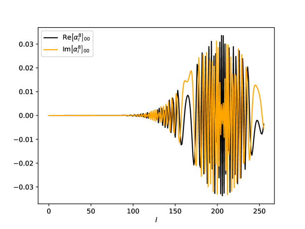
Figure 7. Matrix element $\left[\alpha_{l}^{n}\right]_{pj}$ with $p=j=0$ at scale $n=8$ corresponding to the time step $t=0.0001$ and the MRA order $\mathfrak{k}=6$.

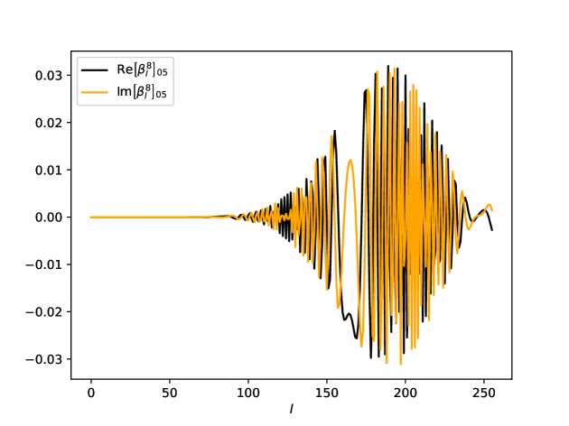
Figure 8. Matrix element $\left[\beta_{l}^{n}\right]_{pj}$ with $p=0$, $j=5$ at scale $n=8$ corresponding to the time step $t=0.0001$ and the MRA order $\mathfrak{k}=6$.

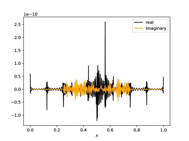
Figure 9. Difference between the analytical solution (6.1) and the numerically propagated one at the time moment $t=0.0001$ for the MRA order $\mathfrak{k}=20$ and the precision $\varepsilon=10^{-10}$.

Figure 10. Convergence comparison between FFT-based schemes (solid lines) and MRA-based schemes (large dots) in the harmonic potential example. The convergence rates are indicated by the dashed lines. The legend corresponds to different integrators: (S2) for (1.4), (A4) for (5.4), (A6) for (5.1), (Y6) for (5.8) with $n=6$ and (Y8) for (5.8) with $n=8$.

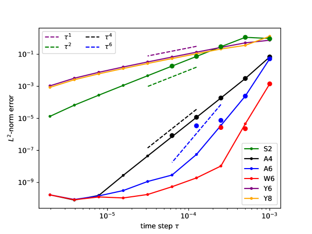
Figure 11. Convergence comparison between FFT-based schemes (solid lines) and MRA-based schemes (large dots) in the Morse potential example. The convergence rates are indicated by the dashed lines. The legend corresponds to different integrators: (S2) for (5.11), (A4) for (5.13), (A6) for (5.15), (W6) for (5.17), (Y6) for (5.12) with $n=6$ and (Y8) for (5.12) with $n=8$.

The free-particle semigroup $\exp\left(it\partial_{x}^{2}\right)$ is encoded in MRCPP (Multiresolution Computation Program Package) [2]. MRCPP is a high-performance C++ library, which provides various tools for working with Multiwavelets in connection to computational chemistry. It is also made available in VAMPyR (Very Accurate Multiwavelets Python Routines) [3], which builds on the MRCPP capabilities, providing an easy to use interface. As an introduction to this software, we refer to our recent article [11], where we have already included a simple numerical experiment with the exponential operator $\exp\left(it\partial_{x}^{2}\right).$ In [11] we did not exploit the sparsity analysed thoroughly here in Subsection 4.1. In order to construct the multiresolution of $\exp\left(it\partial_{x}^{2}\right)$ in an adaptive way, the threshold is set to $\varepsilon/10$ for a given precision $\varepsilon$. In other words matrices $\alpha_{l}^{n}$, $\beta_{l}^{n}$, $\gamma_{l}^{n}$ having the Frobenius norm (4.22) less or equal than $\varepsilon/10$, are ignored in numerical calculations. This choice of threshold is motivated by oscillatory behaviour of the matrix entries $\left[\alpha_{l}^{n}\right]_{pj},\left[\beta_{l}^{n}\right]_{pj},\left[\gamma_{l}^{n}\right]_{pj}$ with respect to the distance to diagonal $l$, on the one hand, see Figures 7, 8 and compare with Figure 2. On the other hand, the result of operator application was controlled by the free-particle analytical solution to (1.3) of the form

$$u(x,t)=\exp\left(it\partial_{x}^{2}\right)\psi_{0}(x)=\left(\frac{1}{2\pi\sigma^{2}}\right)^{1/4}\sqrt{\frac{4\sigma^{2}}{4it+4\sigma^{2}}}e^{-\frac{(x-x_{0})^{2}}{4it+4\sigma^{2}}}$$ (6.1)

associated with the initial condition

$$\psi_{0}(x)=\left(\frac{1}{2\pi\sigma^{2}}\right)^{1/4}\exp\left(-\frac{(x-x_{0})^{2}}{4\sigma^{2}}\right)$$ (6.2)

in the sense $u(x,0)=\psi_{0}(x).$ Indeed, let $x_{0}=0.5$ and $\sigma=0.04$, for example. Then for the MRA order $\mathfrak{k}=20$, time parameter $t=0.0001$ and precision $\varepsilon=10^{-10}$ we have the $L^{2}$-norm of the difference between analytical and numerically propagated solutions equaled $2.0\cdot 10^{-11}$, see Figure 9.

This concludes numerical description of the free-particle propagator. Below we illustrate its use on two toy model problems. Its performance is compared to the periodic spectral method.

6.1. Harmonic potential

Our first numerical example takes the Schrödinger equation

$$i\partial_{t}\psi=-\frac{1}{2}\partial_{x}^{2}\psi+V(x)\psi$$

with the harmonic potential

$$V(x)=V_{0}\left(x-\frac{1}{2}\right)^{2}.$$

It is complemented by the initial condition $\psi(0)=\psi_{0}$ having the Gaussian form (6.2). It is well known that in the harmonic potential the density $\left|\psi(t)\right|^{2}$ oscillates with the period $t_{\text{per}}=\pi\sqrt{2/V_{0}},$ namely, $\psi\left(t_{\text{per}}\right)=-\psi_{0}.$ This comes from the fact that the eigenvalues for the Hamiltonian are $\sqrt{2V_{0}}(n+1/2).$

Ideally, a choice of parameters like $V_{0}$ should be physically motivated. Then given some tolerance one can set the computational domain of size $L$ centered, for our example, at $x=1/2$. Transforming the problem to the unit space interval $[0,1]$, one will obviously get that the final $V_{0}$ turns out to be proportional to $L^{4}$. Therefore, we set the following parameters $V_{0}=98304$, $x_{0}=0.375$ and $\sigma=0.025$ associated with the domain $[0,1]$.

We conduct numerical simulations with time step $\tau$ ranging from $t_{\text{per}}/10$ to $t_{\text{per}}/160$ up to the final time moment $t=t_{\text{per}}$ using the machinery developed here. The integrators in use are referred as follows

1. the simple second order scheme (1.4),

2. the Chin-Chen’s scheme A of fourth order (5.4),

3. the Chin-Chen’s scheme A of sixth order (5.1),

4. the Yoshida’s scheme (5.8) with the order $n=6$,

5. the Yoshida’s scheme (5.8) with the order $n=8$.

The accuracy of the obtained solution $\psi$ for each of these schemes is estimated by the $L^{2}$-difference

$$\text{error}(t)=\left\|\psi(t)-\psi_{\text{ref}}(t)\right\|_{L^{2}(0,1)}.$$ (6.3)

Here we calculate the error at the moment $t=t_{\text{per}}$ with respect to the reference $\psi_{\text{ref}}(t_{\text{per}})=-\psi_{0}.$ For the multiwavelet calculations we take the MRA order $\mathfrak{k}=18$ and the tolerance needed for adaptive resolution to be $\varepsilon=10^{-10}$. The performance is compared with the Fourier spectral method calculations using $1024$ grid points inside of the unit interval $[0,1]$.

The electron dynamics in the harmonic potential well is smooth and it can be viewed as periodic with very high precision. Therefore, there is no surprise that the spectral method outperforms the multiresolution technique in Figure 10. The accuracy stagnation for the FFT based schemes reveals itself at four times smaller time steps than the corresponding stagnation for the MRA based schemes, with $\tau=t_{\text{per}}/640\approx 2.2\cdot 10^{-5}$ compared to $\tau=t_{\text{per}}/160\approx 8.9\cdot 10^{-5}$ for the integrators (A6), (Y6), (Y8). Otherwise, the precision is consistent and the convergence is optimal for each scheme, as indicated by the slopes of curves in Figure 10 corresponding to their theoretical counterparts. It is also interesting to notice that (Y8) does not reach the accuracy of the cheaper scheme (A6) in the current setup.

6.2. Walker-Preston model

In order to test the multiwavelet machinery on the problems with time-dependent Hamiltonian, we consider the Walker-Preston model [39] of a diatomic molecule in a strong laser field. The equation reads

$$i\partial_{t}\psi=-\frac{1}{2}\partial_{x}^{2}\psi+V(x)\psi+\mathcal{E}(x,t)\psi,$$

where $V(x)$ stands for the Morse potential

$$V(x)=V_{0}\left(1-e^{-\alpha x}\right)^{2}$$

with $V_{0}=0.2251\mu$, $\mu=1745$ and $\alpha=1.1741$. These parameters correspond to the HF molecule. Here $\mathcal{E}(x,t)=Ax\cos\omega t$ is the external field with $A=0.011025\mu$ and $\omega=0.01787\mu.$ The first $0\to 1$ vibrational frequency difference in the Morse oscillator is $0.01807\mu,$ so $\omega$ is slightly below resonance. As the initial condition $\psi(0)=\psi_{0}$ we consider the ground state wave function

$$\psi_{0}(x)=\sqrt{\alpha\frac{\xi^{2\lambda-1}(x)}{\Gamma(2\lambda-1)}e^{-\xi(x)}},\quad\xi(x)=2\lambda e^{-\alpha x},\quad\lambda=\frac{\sqrt{2V_{0}}}{\alpha}$$

having the ground state energy

$$E_{0}=\alpha\sqrt{\frac{V_{0}}{2}}-\frac{\alpha^{2}}{8}.$$

It is worth to point out that a direct evaluation of $\psi_{0}(x)$ may lead to huge round up errors. Therefore, we rewrite it in the form suitable for numerical calculations. There is an integer $m\in\mathbb{N}$ such that $2\lambda-1=m+\delta\lambda$ with $1/2\leqslant\delta\lambda<3/2.$ So we can factorise $\psi_{0}$ as

$$\psi_{0}(x)=\sqrt{\alpha\frac{\xi^{\delta\lambda}}{\Gamma(\delta\lambda)}\frac{\xi e^{-\xi/m}}{\delta\lambda}\frac{\xi e^{-\xi/m}}{\delta\lambda+1}\cdot\ldots\cdot\frac{\xi e^{-\xi/m}}{\delta\lambda+m-1}},$$

so eliminating possibility of rounding error.

All the introduced parameters are associated with the computational domain $[-0.8,4.32]$ of the size $L=5.12$, used by many authors [12, 16, 22, 31, 32] for testing different numerical methods. Thus it is known that a use of the spectral periodic treatment for this problem with 64 grid points gives very accurate results, that can be regarded as a perfect benchmark for our purposes. However, in order to be able to exploit the multiresolution technique one needs to translate the formulation to the computational domain $[0,1]$ with an affine transformation. Henceforth $x\in[0,1]$ and the time scales $t=t^{\text{original}}/L^{2}$. All the other units are changed accordingly, for example, the dissociation energy $V_{0}=V_{0}^{\text{original}}L^{2}=0.2251\mu L^{2}$.

Spectral FFT-based simulations are conducted with time step $\tau$ ranging from $0.001$ down to $0.001\cdot 2^{-10}$. The final time moment is set to $t_{\text{fin}}=0.1$. The integrators in use are referred as follows

1. the simple second order scheme (5.11),

2. the Chin-Chen’s scheme A of fourth order (5.13),

3. the Chin-Chen’s scheme A of sixth order (5.15),

4. the Chin-Chen’s scheme A of sixth order (5.17) obtained via the procedure (5.16),

5. the Yoshida’s scheme (5.12) with the order $n=6$,

6. the Yoshida’s scheme (5.12) with the order $n=8$.

The accuracy of the obtained solution $\psi$ for each of these schemes is estimated by (6.3) at the final time moment $t=t_{\text{fin}}$. Now we do not have an analytical result that could stand in place of $\psi_{\text{ref}}$ as in the previous experiment. Presuming we do not know a priori which scheme is the most precise, we take different $\psi_{\text{ref}}$ for each scheme. It is defined by the tiniest small step in use and according to the scheme in question. In other words, $\psi_{\text{ref}}$ for (S2) numerical solutions is the (S2) FFT-based numerical solution associated to the time step $\tau=0.001\cdot 2^{-10}$, and so on. The same references are used later on in order to estimate the accuracy of the corresponding multiwavelet simulations.

In fact we can again see an obvious accuracy outperformance of the periodic spectral method in Figure 11. This time, however, we knew a priori that the best FFT calculations are achieved with the rough grid consisting of only 64 points. Indeed, refining the grid to 256 or 1024 one encounters poorer accuracy due to the Gibbs phenomenon leading to high oscillations of solutions close to the boundary points. It does not affect the multiresolution approach, of course. We do not include figures corresponding to refined grid FFT calculations here, as they exhibit behavior similar to Figure 11. However, these FFT results demonstrate poorer convergence, deviating from the theoretically predicted rate, before the MRA calculations approach stagnation. In other words, FFT-based spectral calculations can yield inferior results compared to MRA-based ones in terms of accuracy.

An interesting and noteworthy outcome is that the extensions (5.12) of Yoshida’s schemes (5.8) for the time-dependent potential case degenerate to first order. According to [40] it may happen that some exponential integrators lose their theoretically predicted accuracy after the Suzuki’s extension described in Subsection 5.2. It seems to us that Yoshida’s schemes (5.8) cannot be efficiently extended to non-autonomous equations. The first author encountered a similar problem before [19].

7. Conclusion

We have developed a multiresolution analysis of the semigroup $\exp\left(it\partial_{x}^{2}\right)$ and introduced MRA-based numerical methods for solving the time-dependent Schrödinger equation. These methods offer several notable advantages. First of all, they can be seamlessly integrated with existing tools for solving stationary problems. Specifically, the application of singular integral operators arising from potential $V$, as utilized in Kohn-Sham and Hartree-Fock theories, is already well-established in multiwavelet bases. Consequently, these techniques can be readily adapted to address time evolution problems. Secondly, these methods offer spatial adaptivity, which is particularly crucial for quantum chemistry simulations. In these simulations, it is essential to handle Coulomb-type singularities and solutions with cusps. Therefore, an automatic grid refinement based on specified precision can be extremely beneficial.

There are some drawbacks to consider. Achieving sparsity in the multiresolution representation of $\exp\left(it\partial_{x}^{2}\right),$ which is obviously needed for efficient computations, requires large time steps $t$ and a high MRA order $\mathfrak{k}$. However, a use of a too large MRA order $\mathfrak{k}$ can slow down simulations, while overly large time steps $t$ may compromise the accuracy of the results obtained.

In the future, we plan to focus on developing artificial boundary conditions for the MRA-based methods introduced here. This approach will enable us to use larger time steps while maintaining accuracy, by confining the computational domain to a relatively compact size. Additionally, it will facilitate the use of reasonable values for $\mathfrak{k}$. The techniques developed will be applied to problems where FFT-based methods encounter challenges, specifically in modeling the attosecond dynamics of electrons in molecules exposed to intense laser pulses.

Declarations

The CRediT taxonomy of contributor roles [5, 13] is applied. The “Investigation” role also includes the “Methodology”, “Software”, and “Validation” roles. The “Analysis” role also includes the “Formal analysis” and “Visualization” roles. The “Funding acquisition” role also includes the “Resources” role. The contributor roles are visualized in the following authorship attribution matrix, as suggested in Ref. [1].

Table 1. Levels of contribution: major, minor.

	ED	YZ	LF
Conceptualization
Investigation
Data curation
Analysis
Supervision
Writing – original draft
Writing – revisions
Funding acquisition
Project administration

Acknowledgments. The authors are grateful to S. R. Jensen and Ch. Tantardini for numerous helpful discussions. The research was supported by the Research Council of Norway through its Centres of Excellence scheme, Hylleraas-senteret, project number 262695.

References

- [1] Researchers are embracing visual tools to give fair credit for work on papers. https://www.natureindex.com/news-blog/researchers-embracing-visual-tools-contribution-matrix-give-fair-credit-authors-scientific-papers. Accessed: 2021-5-3.
- [2] Mrcpp repository, 2024. Accessed: 9 February 2024.
- [3] Vampyr repository, 2024. Accessed: 9 February 2024.
- [4] Abramowitz, M., Ed. Handbook of mathematical functions: with formulas, graphs, and mathematical tables, 10. print., with corr ed. No. 55 in Applied mathematics series. U. S. Government Printing Office, Washington, DC, 1972.
- [5] Allen, L., Scott, J., Brand, A., Hlava, M., and Altman, M. Publishing: Credit where credit is due. Nature 508 (2014), 312–313.
- [6] Alpert, B. A class of bases in for the sparse representation of integral operators. SIAM Journal on Mathematical Analysis 24, 1 (1993), 246–262.
- [7] Alpert, B., Beylkin, G., Gines, D., and Vozovoi, L. Adaptive solution of partial differential equations in multiwavelet bases. Journal of Computational Physics 182, 1 (2002), 149–190.
- [8] Beylkin, G., Coifman, R., and Rokhlin, V. Fast wavelet transforms and numerical algorithms i. Communications on Pure and Applied Mathematics 44, 2 (1991), 141–183.
- [9] Beylkin, G., and Keiser, J. M. On the adaptive numerical solution of nonlinear partial differential equations in wavelet bases. Journal of Computational Physics 132, 2 (1997), 233–259.
- [10] Bischoff, F. A. Chapter one - computing accurate molecular properties in real space using multiresolution analysis. In State of The Art of Molecular Electronic Structure Computations: Correlation Methods, Basis Sets and More, L. U. Ancarani and P. E. Hoggan, Eds., vol. 79 of Advances in Quantum Chemistry. Academic Press, 2019, pp. 3–52.
- [11] Bjørgve, M., Tantardini, C., Jensen, S. R., Gerez S., G. A., Wind, P., Di Remigio Eikås, R., Dinvay, E., and Frediani, L. VAMPyR—A high-level Python library for mathematical operations in a multiwavelet representation, 04 2024.
- [12] Blanes, S., and Moan, P. Splitting methods for the time-dependent schrödinger equation. Physics Letters A 265, 1 (2000), 35–42.
- [13] Brand, A., Allen, L., Altman, M., Hlava, M., and Scott, J. Beyond authorship: attribution, contribution, collaboration, and credit. Learn. Publ. 28 (2015), 151–155.
- [14] Chin, S. A. Symplectic integrators from composite operator factorizations. Physics Letters A 226, 6 (1997), 344–348.
- [15] Chin, S. A., and Chen, C. R. Fourth order gradient symplectic integrator methods for solving the time-dependent Schrödinger equation. The Journal of Chemical Physics 114, 17 (05 2001), 7338–7341.
- [16] Chin, S. A., and Chen, C. R. Gradient symplectic algorithms for solving the Schrödinger equation with time-dependent potentials. The Journal of Chemical Physics 117, 4 (07 2002), 1409–1415.
- [17] Coccia, E., and Luppi, E. Time-dependent ab initio approaches for high-harmonic generation spectroscopy. Journal of Physics: Condensed Matter 34, 7 (nov 2021), 073001.
- [18] Cohen, A., Daubechies, I., and Feauveau, J.-C. Biorthogonal bases of compactly supported wavelets. Communications on Pure and Applied Mathematics 45, 5 (1992), 485–560.
- [19] Dinvay, E., Kalisch, H., and Părău, E. I. Fully dispersive models for moving loads on ice sheets. Journal of Fluid Mechanics 876 (2019), 122–149.
- [20] Evans, L. C. Partial differential equations, 2nd ed ed. No. v. 19 in Graduate studies in mathematics. American Mathematical Society, Providence, R.I, 2010. OCLC: ocn465190110.
- [21] Fann, G., Beylkin, G., Harrison, R. J., and Jordan, K. E. Singular operators in multiwavelet bases. IBM Journal of Research and Development 48, 2 (2004), 161–171.
- [22] Gray, S. K., and Verosky, J. M. Classical Hamiltonian structures in wave packet dynamics. The Journal of Chemical Physics 100, 7 (04 1994), 5011–5022.
- [23] Harrison, R. J., Fann, G. I., Yanai, T., Gan, Z., and Beylkin, G. Multiresolution quantum chemistry: Basic theory and initial applications. The Journal of Chemical Physics 121, 23 (11 2004), 11587–11598.
- [24] Jensen, S. R., Saha, S., Flores-Livas, J. A., Huhn, W., Blum, V., Goedecker, S., and Frediani, L. The elephant in the room of density functional theory calculations. The Journal of Physical Chemistry Letters 8, 7 (2017), 1449–1457. PMID: 28291362.
- [25] Kaye, J., Barnett, A., and Greengard, L. A high-order integral equation-based solver for the time-dependent schrödinger equation. Communications on Pure and Applied Mathematics 75, 8 (2022), 1657–1712.
- [26] Luca Frediani, Eirik Fossgaard, T. F., and Ruud, K. Fully adaptive algorithms for multivariate integral equations using the non-standard form and multiwavelets with applications to the poisson and bound-state helmholtz kernels in three dimensions. Molecular Physics 111, 9-11 (2013), 1143–1160.
- [27] Mallat, S. G. Multiresolution approximations and wavelet orthonormal bases of . Transactions of the American mathematical society 315, 1 (1989), 69–87.
- [28] Mallat, S. G. A theory for multiresolution signal decomposition: the wavelet representation. IEEE transactions on pattern analysis and machine intelligence 11, 7 (1989), 674–693.
- [29] Mourou, G. Nobel lecture: Extreme light physics and application. Rev. Mod. Phys. 91 (Jul 2019), 030501.
- [30] Nisoli, M., Decleva, P., Calegari, F., Palacios, A., and Martín, F. Attosecond electron dynamics in molecules. Chemical Reviews 117, 16 (2017), 10760–10825. PMID: 28488433.
- [31] Peskin, U., Kosloff, R., and Moiseyev, N. The solution of the time dependent Schrödinger equation by the method: The use of global polynomial propagators for time dependent Hamiltonians. The Journal of Chemical Physics 100, 12 (06 1994), 8849–8855.
- [32] Sanz‐Serna, J. M., and Portillo, A. Classical numerical integrators for wave‐packet dynamics. The Journal of Chemical Physics 104, 6 (02 1996), 2349–2355.
- [33] Strickland, D. Nobel lecture: Generating high-intensity ultrashort optical pulses. Rev. Mod. Phys. 91 (Jul 2019), 030502.
- [34] Suzuki, M. General theory of higher-order decomposition of exponential operators and symplectic integrators. Physics Letters A 165, 5 (1992), 387–395.
- [35] Suzuki, M. General decomposition theory of ordered exponentials. Proceedings of the Japan Academy, Series B 69, 7 (1993), 161–166.
- [36] Suzuki, M. New scheme of hybrid exponential product formulas with applications to quantum monte-carlo simulations. In Computer Simulation Studies in Condensed-Matter Physics VIII (Berlin, Heidelberg, 1995), D. P. Landau, K. K. Mon, and H.-B. Schüttler, Eds., Springer Berlin Heidelberg, pp. 169–174.
- [37] Tantardini, C., Dinvay, E., Pitteloud, Q., Gerez S., G. A., Jensen, S. R., Wind, P., Remigio, R. D., and Frediani, L. Advancements in quantum chemistry using multiwavelets: Theory, implementation, and applications. In preparation, 2024.
- [38] Vence, N., Harrison, R., and Krstić, P. Attosecond electron dynamics: A multiresolution approach. Phys. Rev. A 85 (Mar 2012), 033403.
- [39] Walker, R. B., and Preston, R. K. Quantum versus classical dynamics in the treatment of multiple photon excitation of the anharmonic oscillator. The Journal of Chemical Physics 67, 5 (09 1977), 2017–2028.
- [40] Wiebe, N., Berry, D., Høyer, P., and Sanders, B. C. Higher order decompositions of ordered operator exponentials. Journal of Physics A: Mathematical and Theoretical 43, 6 (jan 2010), 065203.
- [41] Yin, J. A fourth-order compact time-splitting method for the dirac equation with time-dependent potentials. Journal of Computational Physics 430 (2021), 110109.
- [42] Yoshida, H. Construction of higher order symplectic integrators. Physics Letters A 150, 5 (1990), 262–268.