Conformalized Physics-Informed Neural Networks
Abstract
Physics-informed neural networks (PINNs) are an influential method of solving differential equations and estimating their parameters given data. However, since they make use of neural networks, they provide only a point estimate of differential equation parameters, as well as the solution at any given point, without any measure of uncertainty. Ensemble and Bayesian methods have been previously applied to quantify the uncertainty of PINNs, but these methods may require making strong assumptions on the data-generating process, and can be computationally expensive. Here, we introduce Conformalized PINNs (C-PINNs) that, without making any additional assumptions, utilize the framework of conformal prediction to quantify the uncertainty of PINNs by providing intervals that have finite-sample, distribution-free statistical validity.
1 Introduction
Physics-informed neural networks are an influential method developed by Raissi et al. (2019), which employs neural networks to solve a differential equation (forward problem) well as estimate its parameters (inverse problem). The differential equation (DE) may be ordinary (ODE) or partial (PDE). PINNs have been extended in many ways (e.g. UPINNs by Podina et al. (2023) for learning functions, XPINNs by Jagtap & Karniadakis (2021) for domain decomposition, and DeepONets by Lu et al. (2021) for operator learning), in order to solve increasingly complex problems. However, many of these methods produce only point estimates of the DE solution. This makes it difficult to apply these methods in any practical situation where the error of the solution needs to be quantified or bounded.
Uncertainty quantification methods for PINNs have been developed in order to fill this gap, such as Bayesian PINNs in Yang et al. (2021). This method involves modelling the uncertainty of model and DE parameters using Bayesian statistics. However, this approach has several significant drawbacks. An appropriate prior distribution on the neural network and DE parameters must be determined in advance, and in the case of model misspecification at this stage, the resulting uncertainties may not be calibrated, as shown by Fong & Holmes (2021). Secondly, as described in Yang et al. (2021), the noise distribution within the data needs to be assumed in advance. In Yang et al. (2021), a Gaussian noise model is assumed, but may not be an appropriate model in all cases.
Conformal prediction (CP), as introduced by Vovk et al. (2005), is a user-friendly framework for creating uncertainty intervals on predictions made by any machine learning model, including ones that are black-box or not inherently interpretable. Its distinctive feature lies in the ability to provide intervals that have finite-sample, distribution-free statistical validity. This implies that the method offers explicit and non-asymptotic guarantees without relying on specific distributional or model-related assumptions. This makes conformal prediction a versatile tool that can be applied to any model, including neural networks. The most common flavor of CP methods is the Split Conformal method as outlined by Papadopoulos et al. (2002), which splits the otherwise training set into training and calibration sets; it then uses the former to train a point predictor and the latter to construct uncertainty intervals.
Here, we introduce Conformalized PINNs (C-PINNs) and show how they can quantify the uncertainty of: (1) the inferred DE solution (the forward problem) and (2) estimated DE parameters (the inverse problem). We also show how a procedure that utilizes the strong law of large numbers and an underlying property of Split Conformal methods can be used to rigorously check the exact coverage validity of C-PINN intervals.
2 Methodology and Results
For the forward and inverse problems, we consider the logistic growth Ordinary Differential Equation (ODE). This equation is widely used to model logistic growth as described by West & Newton (2019); Kohandel et al. (2006) (e.g. in a context where cells () are growing over time () but are limited by the nutritional value of the medium):
| (1) |
In Section 2.1, we fix the value of and the initial condition , and show the coverage validity of the solution intervals inferred by a Conformalized Physics-Informed Neural Network (C-PINN), for both noise-free and noisy datasets. In Section 2.2, we focus on the inverse problem and show a similar validity for parameter intervals. Model training and architectures are described in Appendix A.2.
For the forward problem only, we also consider the 1D Buckley-Leverett Equation Wang et al. (2021):
| (2) |
taking . Li & Mei (2021) showed that a continuous PINN was not able to successfully learn the solution to the equation, likely due to the discontinuous nature of the solution. To see if conformal prediction can still be used to construct intervals with valid coverage when PINNs do not approximate the solution well, we conformalize the forward problem for eq. 2 in Section 2.1.2.
2.1 Conformalizing the PINN surrogate solution (forward problem)
In the following two subsections, we conformalize the forward problem for the logistic growth ODE (Section 2.1.1) and a PDE with a discontinuous solution, the 1D Buckley-Leverett equation (Section 2.1.2).
2.1.1 Conformalizing the logistic growth ODE
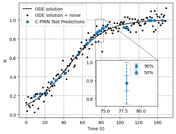
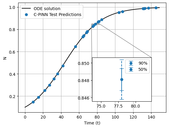
First, a numerical solver is used to solve Equation 1 for the initial condition and for time 0 to 150. A dataset of 150 tuples are generated in total. Gaussian noise (noise level 0.08 as per Podina et al. (2023)) is added to the solution. These are randomly split into holdout set of points (100), training points (25), and test points (25). Then, a single continuous PINN is fit to the training data as per Raissi et al. (2019), with the parameter value of given to the PINN in advance. After solving the forward problem, the PINN returns a surrogate solution to the differential equation. Since the solution is modelled using a neural network, it can be evaluated at any time, not just at the training time.
We implement split conformal prediction as per Papadopoulos et al. (2002) on the solution generated by PINNs (Fig 1(a)). Given a prespecified miscoverage level , this procedure creates a -confidence interval for a new test point which will contain the true label with probability as derived in Angelopoulos & Bates (2021). This means the constructed interval has valid coverage. The 90% and 50% confidence intervals (with miscoverage levels respectively) seen in the inset of Fig 1(a) are guaranteed to contain at least 90% and 50% of the true labels respectively.
In order to create a prediction interval (of confidence ) for a new test point , we split the holdout set of 100 tuples into calibration points and validation points. We then evaluate a non-conformity score for each calibration point. To create the scores, for each tuple of the calibration points, we evaluate the absolute error between each true , and the corresponding predicted . With miscoverage value (and corresponding confidence level 90%), we calculate the th quantile of the calibration non-conformity scores. For a new prediction , we can use the interval as the 90% confidence interval. Any interval generated this way via split conformal prediction is proven to have valid coverage as per Angelopoulos & Bates (2021).
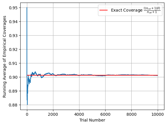
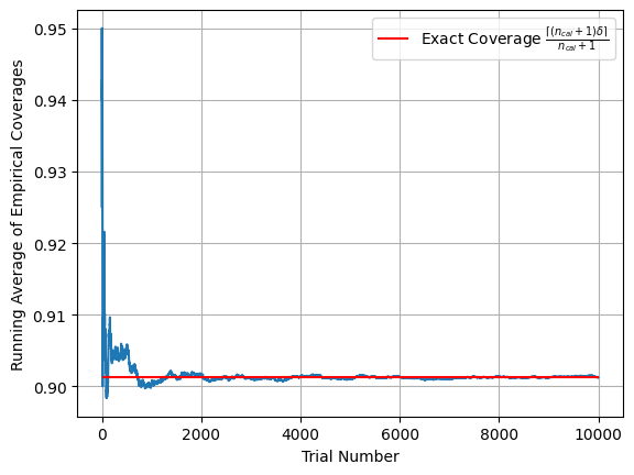
We then empirically show that the 90% interval has valid coverage (Fig 1(b)). To do this, we perform split conformal prediction over many different splits of the validation and calibration points. This procedure is outlined in Angelopoulos & Bates (2021). After constructing the interval using the calibration set, we check how many of the validation points in fact fall in the constructed interval. Angelopoulos & Bates (2021) also shows that for calibration points and miscoverage level , the coverage of the split conformal interval is exactly . Fig 1(b) shows that the mean coverage converges to exactly this coverage over 10000 random splits (trials), which implies that the constructed intervals are valid.
Hence, conformal prediction can be used to quantify the uncertainty and fit of a PINN solution even when there is only a single dataset available (with significant noise). Furthermore, the method yields valid coverage, which we have verified rigorously. We repeat this procedure for noiseless data, showing the fit and coverage convergence in Fig 5. The predicted 90% and 50% confidence intervals are much smaller since the PINN is better able to predict on an unseen test point . However, we still have valid coverage as can be seen in Fig 5(b). Hence, this method can be used to quantify the performance of the PINN on unseen test data, which is a good measure of the generalization of the solution.
2.1.2 Conformalizing a PDE with a discontinous solution (Buckley-Leverett Equation)
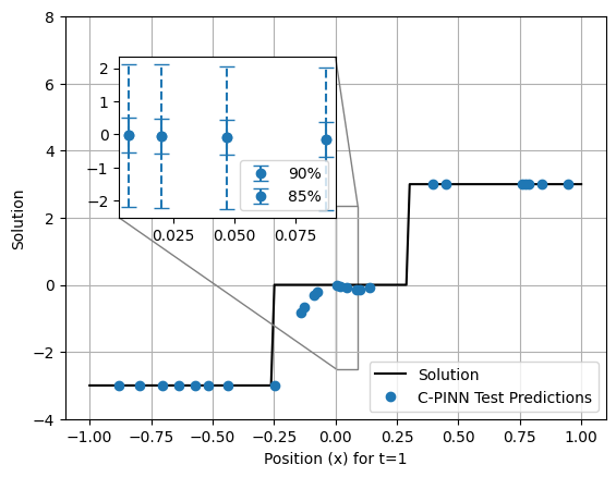
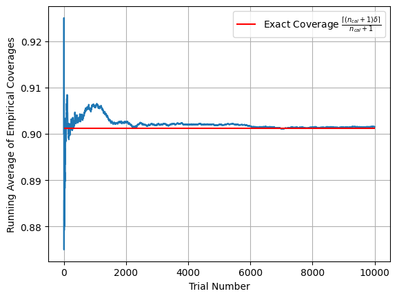
We conformalize the forward problem as before for the Buckley-Leverett equation. A PINN is used to solve eq. 2 with 25 noiseless training points for . The resulting solution matches the training data, but does not adequately represent the solution near discontinuities at . Fig 2(a) shows the true and predicted solution, along with the 90% and 85% confidence intervals. However, since the model only performs poorly at discontinuities, adaptive intervals would be more informative. The coverage is still as expected despite the PINN’s poor performance in recovering the true solution (Fig 2(b)).
2.2 Conformalizing an ODE parameter estimate (inverse problem)
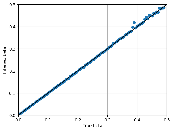
In this section, we conformalize the inverse problem. Suppose that we are tasked with providing a valid interval over for a new dataset , given a distribution over possible datasets . In the simplest form, which we explore here, the given distribution is a distribution over possible . Then, the C-PINN can be used to construct a valid interval over the estimate for . We outline the procedure to do this, and show that the method has valid coverage.
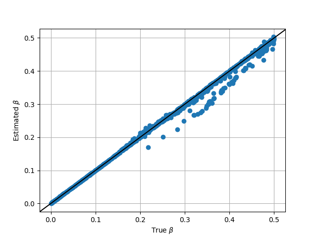
To conformalize a new estimate, we generate holdout pairs (sampled true , generated datasets using , inferred of ), shown in Fig 3(a). We sample 1000 times from the given distribution, which we assume is Uniform. We then solve Eq 1 via an ODE solver for these values of , generating 10 points per dataset. We obtain a set of 1000 tuples . Then, for each , we employ a standard continuous PINN to estimate the parameter in Eq 1. This yields one estimate per dataset. Since each PINN can only infer after being trained on a specific dataset, we must use a separately initialized PINN to find for each dataset. We explore alternative model options in the Conclusion section.
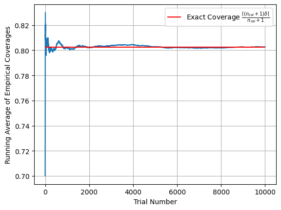
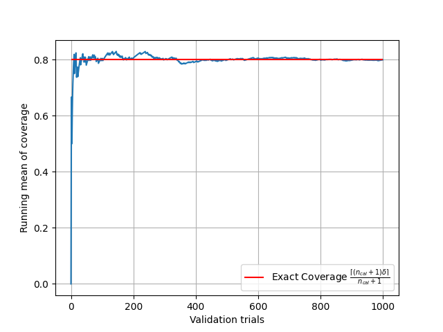
We perform split conformal prediction using the previously generated holdout set. For a new dataset , we first use a PINN to estimate for the dataset . Then, we sample 800 points from the holdout set to form the calibration set, and construct an 80% confidence interval as per Section 2.1. The interval given by the C-PINN will have valid coverage as long as in fact comes from the given distribution (Uniform in this case).
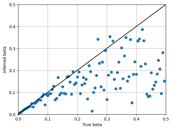
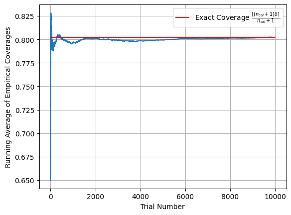
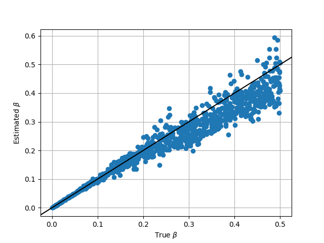
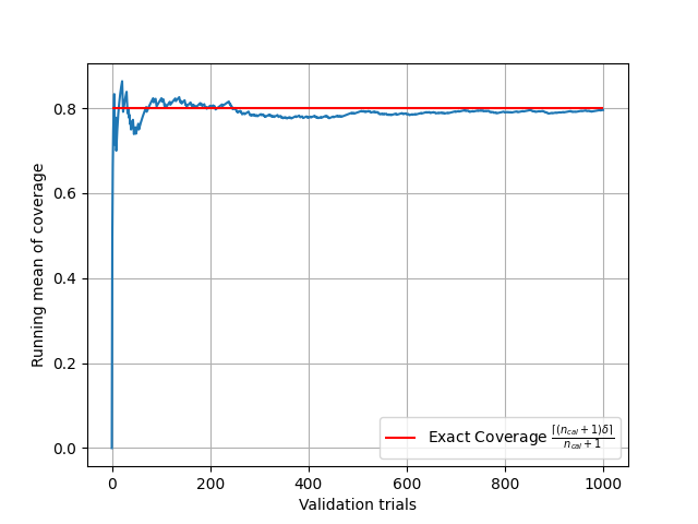
The mean interval coverage converges to the expected coverage (Fig 3(b)) over many validation points . To compute the coverage, we repeatedly sample a new with and compute the proportion of the time that falls in the constructed interval. We note that for a smaller holdout set, different confidence level, and for a different distribution of , the coverage would still be valid due to exchangeability, as discussed in Angelopoulos & Bates (2021). We repeat this experiment with noisy data (Fig 6(a), 6(b)) and obtain similarly valid coverage, since each dataset is still sampled i.i.d. Additionally, we obtain valid coverage upon repeatedly splitting the holdout set into validation and calibration points, as per Section 2.1 (Figure 7 and 8 in Appendix A.4).
3 Conclusion and Discussion
In this work, we conformalize physics-informed neural networks (PINNs) in two ways: first, we conformalize the surrogate solution of the logistic growth ODE and the Buckley-Leverett PDE (Eqs. 1 and 2, forward problem) using a holdout calibration set and split conformal prediction as per Papadopoulos et al. (2002). In order to validate the method, we employ an averaging approach to compute the coverage of the intervals over many calibration/validation splits. Even when the data is significantly noisy, we show that the empirical coverage converges to the the theoretical coverage. Secondly, we conformalize one inferred parameter (Eq 1, inverse problem). We use the parameter estimates from many PINNs to conformalize the parameter estimate for a new dataset. The resulting interval provides valid coverage for a new, unseen value of . In order to reduce the computational cost of this method, we note that it is possible to use UPINNs as introduced by Podina et al. (2023) to infer for several datasets simultaneously. Further extensions to this work include creating adaptive conformal prediction intervals for PINNs, which would tailor the interval size based on the input to the model. Another possibility is to conformalize UPINNs using split conformal prediction.
References
- Angelopoulos & Bates (2021) Anastasios N Angelopoulos and Stephen Bates. A gentle introduction to conformal prediction and distribution-free uncertainty quantification. arXiv preprint arXiv:2107.07511, 2021.
- Fong & Holmes (2021) Edwin Fong and Chris C Holmes. Conformal bayesian computation. Advances in Neural Information Processing Systems, 34:18268–18279, 2021.
- Jagtap & Karniadakis (2021) Ameya D Jagtap and George E Karniadakis. Extended physics-informed neural networks (xpinns): A generalized space-time domain decomposition based deep learning framework for nonlinear partial differential equations. In AAAI spring symposium: MLPS, volume 10, 2021.
- Kingma & Ba (2014) Diederik P Kingma and Jimmy Ba. Adam: A method for stochastic optimization. arXiv preprint arXiv:1412.6980, 2014.
- Kohandel et al. (2006) M Kohandel, S Sivaloganathan, and A Oza. Mathematical modeling of ovarian cancer treatments: sequencing of surgery and chemotherapy. Journal of theoretical biology, 242(1):62–68, 2006.
- Li & Mei (2021) Ying Li and Fangjun Mei. Deep learning-based method coupled with small sample learning for solving partial differential equations. Multimedia Tools and Applications, 80(11):17391–17413, 2021.
- Lu et al. (2021) Lu Lu, Pengzhan Jin, Guofei Pang, Zhongqiang Zhang, and George Em Karniadakis. Learning nonlinear operators via deeponet based on the universal approximation theorem of operators. Nature machine intelligence, 3(3):218–229, 2021.
- Papadopoulos et al. (2002) Harris Papadopoulos, Kostas Proedrou, Volodya Vovk, and Alex Gammerman. Inductive confidence machines for regression. In Machine Learning: ECML 2002: 13th European Conference on Machine Learning Helsinki, Finland, August 19–23, 2002 Proceedings 13, pp. 345–356. Springer, 2002.
- Paszke et al. (2019) Adam Paszke, Sam Gross, Francisco Massa, Adam Lerer, James Bradbury, Gregory Chanan, Trevor Killeen, Zeming Lin, Natalia Gimelshein, Luca Antiga, et al. Pytorch: An imperative style, high-performance deep learning library. Advances in neural information processing systems, 32, 2019.
- Podina et al. (2023) Lena Podina, Brydon Eastman, and Mohammad Kohandel. Universal physics-informed neural networks: symbolic differential operator discovery with sparse data. In International Conference on Machine Learning, pp. 27948–27956. PMLR, 2023.
- Raissi et al. (2019) Maziar Raissi, Paris Perdikaris, and George E Karniadakis. Physics-informed neural networks: A deep learning framework for solving forward and inverse problems involving nonlinear partial differential equations. Journal of Computational physics, 378:686–707, 2019.
- Vovk et al. (2005) Vladimir Vovk, Alexander Gammerman, and Glenn Shafer. Algorithmic learning in a random world, volume 29. Springer, 2005.
- Wang et al. (2021) Sifan Wang, Yujun Teng, and Paris Perdikaris. Understanding and mitigating gradient flow pathologies in physics-informed neural networks. SIAM Journal on Scientific Computing, 43(5):A3055–A3081, 2021.
- West & Newton (2019) Jeffrey West and Paul K Newton. Cellular interactions constrain tumor growth. Proceedings of the National Academy of Sciences, 116(6):1918–1923, 2019.
- Yang et al. (2021) Liu Yang, Xuhui Meng, and George Em Karniadakis. B-pinns: Bayesian physics-informed neural networks for forward and inverse pde problems with noisy data. Journal of Computational Physics, 425:109913, 2021.
Appendix A Appendix
A.1 Conformalized forward problem: Noiseless data
A.2 Model architecture and training
The physics-informed neural network was implemented in PyTorch (Paszke et al. (2019)) similarly to https://github.com/jayroxis/PINNs. The neural network that was used to model the surrogate solution contains one input, 2 hidden layers with 10 hidden units each, and one output. The activation function used between layers is tanh. In order to train the PINN, the Adam (Kingma & Ba (2014)) optimizer (with default parameters and linear annealing learning rate scheduling) was run for 100 epochs, and then the L-BFGS optimizer was run until convergence.
A.3 Conformalized inverse problem: noisy data
A.4 Conformalized inverse problem: repeated validation/calibration splits
When conformalizing the inverse problem, in addition to testing our method on repeated i.i.d. validation samples as described in Section 2.2, we also show valid coverage using the averaging method described in Section 2.1.