11email: vardi@cs.rice.edu, l.martinelli.tabajara@gmail.com, yl182@rice.edu
Dynamic Programming for Symbolic Boolean Realizability and Synthesis111This is the full version of this paper, with appendices included.
Abstract
Inspired by recent progress in dynamic programming approaches for weighted model counting, we investigate a dynamic-programming approach in the context of boolean realizability and synthesis, which takes a conjunctive-normal-form boolean formula over input and output variables, and aims at synthesizing witness functions for the output variables in terms of the inputs. We show how graded project-join trees, obtained via tree decomposition, can be used to compute a BDD representing the realizability set for the input formulas in a bottom-up order. We then show how the intermediate BDDs generated during realizability checking phase can be applied to synthesizing the witness functions in a top-down manner. An experimental evaluation of a solver – DPSynth – based on these ideas demonstrates that our approach for Boolean realizabilty and synthesis has superior time and space performance over a heuristics-based approach using same symbolic representations. We discuss the advantage on scalability of the new approach, and also investigate our findings on the performance of the DP framework.
Keywords:
Boolean synthesis Binary decision diagram Dynamic programming Bucket elimination.1 Introduction
The Boolean-Synthesis Problem [19] – a fundamental problem in computer-aided design – is the problem of taking in a declarative boolean relation between two sets of boolean variables – input and output – and generating boolean functions, called witness functions, that yield values to the output variables with respect to the input variables so as to satisfy the boolean relation. As a fundamental problem in computer-aided design, there are many applications of boolean synthesis in circuit design. For example, based on a circuit’s desired behavior, we can use boolean synthesis to automatically construct the missing components of the circuit [3]. In addition to being used in circuit design, boolean synthesis has recently found applications also in temporal synthesis [30, 29], where the goal is to construct a a sequential circuit that responds to environment inputs in a way that is guaranteed to satisfy given temporal-logic specification.
Many approaches have been investigated for boolean synthesis, such as knowledge compilation [1], QBF solving [23], and machine learning [17, 18]. Here we build on previous work on boolean synthesis using Binary Decision Diagrams (BDDs) [27]. The main advantage of the decision-diagram approach is that it provides not just the synthesized witness functions, but also the realizability set of the specification, which is the set of inputs with respect to which the specification is realizable. In modular circuit design [19], where a system is composed of multiple modules that are independently constructed, it is imperative to confirm the realizability set of a module, as it has to match the output set of prior modules. Similarly, in the context of temporal synthesis [30, 29], the winning set is constructed iteratively by taking the union of realizability sets, where for each realizability set we construct a witness function. The winning strategy is then constructed by stitching together all these witness functions.
Motivated by applications that require the computation of both realizability sets and witness functions, we describe here a decision-diagram approach that can also handle partially realizable specifications, where the realizability set is neither empty nor necessarily universal. (Indeed, in our benchmark suit, about 30% of the benchmarks are partially realizable.) Our tool, DPSynth computes the realizability sets and witness functions with respects to these sets. While several recent synthesis tools do provide witnesses for partially-realizable specifications, cf. [1, 17, 18], not all of them directly output the realizability set, requiring it, instead, to be computed from the witnesses and the original formula.
The boolean-synthesis problem starts with a boolean formula over sets of input and output variables. The goal is to construct boolean formulas, called witness functions (sometimes called Skolem functions) [18, 1] – for the output variables expressed in terms of the input variables. The BDD-based approach to this problem [15] constructs the BDD for , and then quantifies existentially over the variables to obtain a BDD over the variables that captures the realizability set – the set of assignments in for which an assignment in exists where . The witness functions can then be constructed by iterating over the intermediate steps of the realizability computation [15].
A challenge of this BDD-based approach is that it is often infeasible to construct the BDD . Factored Boolean Synthesis [27] assumes that the formula is given in conjunctive normal form (CNF), where the individual clauses are called factors. Rather than constructing the monolithic BDD , this approach constructs a BDD for each factor, and then applies conjunction in a lazy way and existential quantification in an eager way, using various heuristics to order conjoining and quantifying. As shown in [27], the factored approach, Factored RSynth, is more scalable than the monolithic approach, RSynth. Thus, we use here Factored RSynth as the baseline for comparison in this paper.
By dynamic programming we refer to the approach that simplifies a complicated problem by breaking it down into simpler sub-problems in a recursive manner [5]. Unlike search-based approaches to Boolean reasoning, cf. [21], which directly manipulate truth assignments, we use data structure based on decision diagrams [7] that represents sets of truth assignments. This approach is referred to as symbolic, going back to [11].
The symbolic dynamic-programming approach we propose here is inspired by progress in weighted model counting, which is the problem of counting the number of satisfying (weighted) assignments of boolean formulas. Dudek, Phan, and Vardi proposed in [14], an approach based on Algebraic Decision Diagrams, which are the quantitative variants of BDDs [4]. Dudek et al. pointed out that a monolithic approach is not likely to be scalable, and proposed a factored approach, ADDMC, analogous to the approach in [27], in which conjunction is done lazily and quantification eagerly. In follow-up work [12], they proposed a more systematic way to order the quantification and conjunction operations, based on dynamic programming over project-join trees; the resulting tool, DPMC, was shown to scale better than ADDMC. In further follow-on work, they proposed graded project-join trees for projected model counting, where the input formula has two sets of variables – quantified variables and counting variables [13]. Graded project-join tree offers a recursive decomposition of the Boolean-Synthesis Problem into smaller tasks of projections and join.
We show here how symbolic dynamic programming over graded project-join trees can be applied to boolean synthesis. In our approach, realizability checking is done using a BDD-based bottom-up execution, analogous to the handling of counting quantifiers in [13]. This enables us to compute the realizability set and check its nonemptiness. We then present a novel algorithm for synthesizing the witness functions using top-down execution on graded project-join trees. (In contrast, [13] both types of quantifiers are handled bottom-up). We demonstrate the advantage of our bottom-up-top-down approach by developing a tool, DPSynth. For a fair evaluation, we compare its performance to Factored RSynth, which can also handle partially realizable specifications.
The main contributions of this work are as follows. First, we show how to adapt the framework of projected counting to Boolean synthesis. In projected counting there are two types of existential quantifiers – additive and disjunctive [13], while Boolean synthesis combine universal and existential quantifiers. Second, projected counting requires only a bottom-up pass over the graded project-join trees, while here we introduce an additional, top-down pass over the tree to perform the major part of boolean synthesis, which is,witness construction.
The organization of the paper is as follows. After preliminaries in Section 2, we show in Section 3 how to use graded project-join trees for boolean realizability checking, and show that DPSynth generally scales better than Factored RSynth. Then, in Section 4, we show how to extend this approach from realizability checking to witness-function construction. Experimental evaluation shows that DPSynth generally scales better than Factored RSynth also for witness-function construction. We offer concluding remarks in Section 6.
2 Preliminary Definitions
2.1 Boolean Formula and Synthesis Concepts
A boolean formula , over a set of variables, represents a boolean function , which selects subsets of . A truth assignment satisfies iff . A boolean formula in conjunctive normal form (CNF) is a conjunction of clauses, where a clause is a disjunction of literals (a boolean variable or its negation). When is in CNF, we abuse notation and also use to denote its own set of clauses. Given a CNF formula over input and output variable and , the realizability set of , denoted , is the set of assignments for which there exists an assignment such that . When is clear from context, we simply denote the realizability set by .
Definition 1 (Realizability).
Let be a CNF formula with and as input and output variables. We say that is fully realizable if . We say that is partially realizable if . Finally, we say that is nullary realizable if .
Given the condition that the formula is at least partially realizable, the boolean synthesis problem asks for a set of witnesses for the output variables generated on top of given input values, such that the formula is satisfied. This sub-problem of constructing witnesses, is usually referred to as synthesis.
The motivation behind synthesizing partially-realizable specifications is that there are cases where a specification is not fully realizable, but it is still useful to synthesize a function that works for all inputs in the realizability set. An example is the factorization benchmark family, as discussed in the introduction of [3], which takes an integer and aims to factor it into two integers that are both not equal to 1. If the integer is prime, then there is no valid factorization for this particular input, but it would still be valuable to have a solution that works for all composite numbers. This is why our attention to partially-realizable cases is a contribution of the paper, while related works tend to focus mostly on fully-realizable instances.
Definition 2 (Witnesses in Boolean Synthesis Problem).
Let denote a fully or partially realizable boolean formula with input variables in and output variables , and let be its realizability set. A sequence of boolean functions is a sequence of witness functions for the variables in if for every assignment , we have that holds.
Definition 3 (Synthesis).
Given a partially or fully realizable CNF formula with input and output variables and , the synthesis problem asks to algorithmically construct a set of witness functions for the variables in terms of the variables.
2.2 Dynamic Programming Concepts - Project-Join Trees
A binary decision diagrams (BDD) [7] is directed acyclic graphs with two terminals labeled by and . A BDD provides a canonical representation of boolean functions (and, by extension, boolean formulas). A (reduced, ordered) BDD is constructed from a binary decision tree, using a uniform variable order, of a boolean function by merging identical sub-trees and suppressing redundant nodes (nodes where both children are the same). Each path from the root of the BDD to the 1-terminal represents a satisfying assignment of the boolean function it represents. Based on the combination of BDDs and project-join trees, which is to be defined below, our dynamic-programming algorithm solves the boolean synthesis problem.
Definition 4 (Project-Join Tree of a CNF formula).
A project-join tree [12] for a CNF formula is defined as a tuple , where
-
1.
is a tree with a set of vertices, a set of leaves, and a root
-
2.
is a bijection that maps the leaves of to the clauses of
-
3.
is a function which labels internal nodes with variable sets, where the labels form a partition of , and
-
4.
If a clause contains a variable that belongs to the label of an internal node , then the associated leaf node must descends from .
A Graded Project-Join Tree [13] is a generalization of project-join trees.
Definition 5 (Graded Project-Join Tree of a CNF formula [13]).
A project-join tree of a CNF formula over variables , where , is (, )-graded if there exist grades that partition the internal nodes , such that:
-
1.
For a node, its grade is always consistent with its labels. i.e., If then , and if then .
-
2.
If and , then is not a descendant of in .
Intuitively, in a graded project-join tree, the nodes are partitioned according to a partition of the variables, with nodes in the block always appearing higher than nodes in the block. As we shall see, this is useful for formulas with two different types of quantifiers.
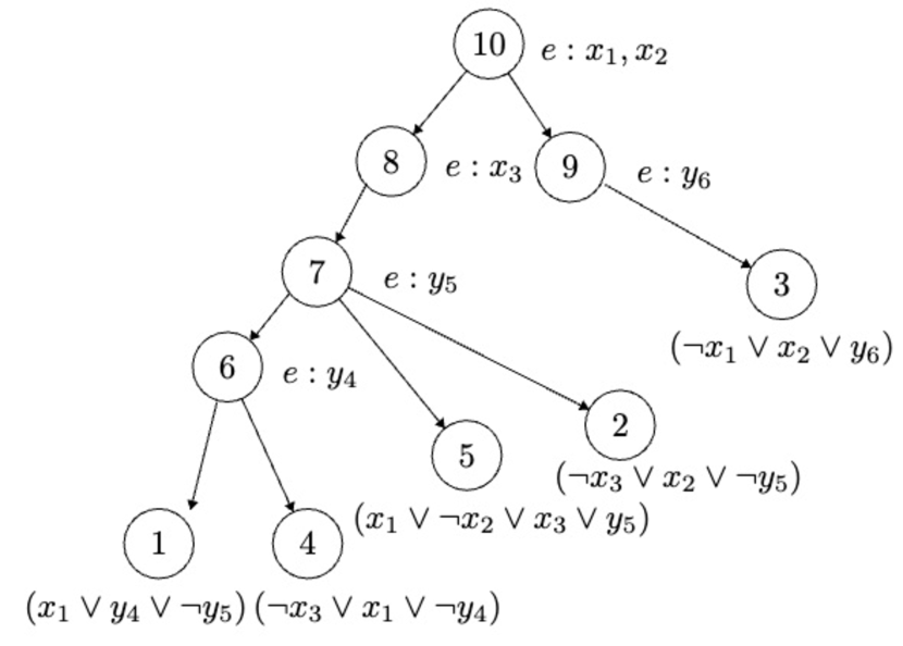
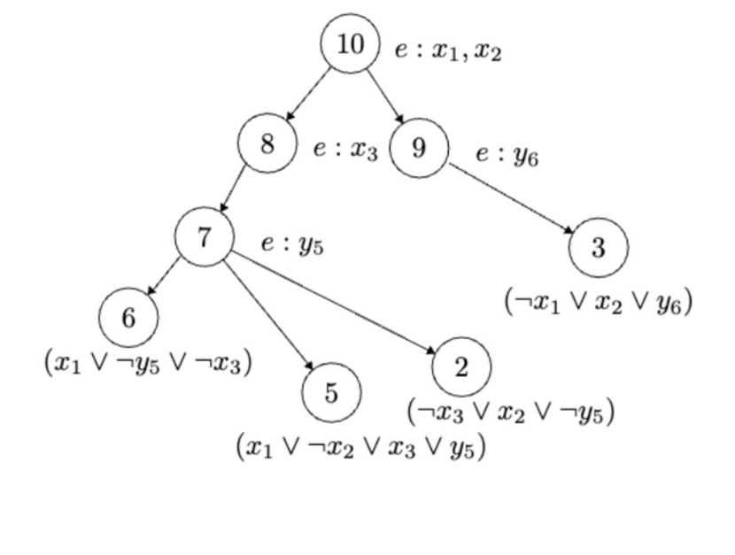
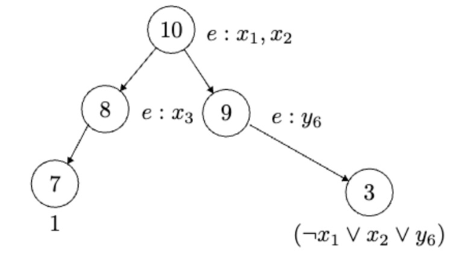
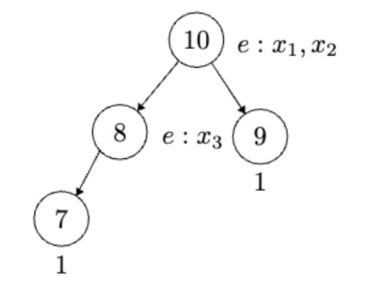
Figure 1 shows an example Graded Project-Join Tree for a CNF formula, along with intermediate trees produced in the course of the execution of our synthesis algorithm. In the upcoming sections we will refer back to this example to illustrate the individual steps of the algorithm related to each intermediate tree.
3 Realizability Checking222Proofs for all lemmas and theorems can be found in the Appendix A.
Our overall approach has three phases: (1) planning – constructing graded project-join trees, (2) realizability checking, and (3) witness-function synthesis. The focus in this section is on realizability checking. We construct the realizability set for an input formula , and then use it to check for full and partial realizability, as described in Definition 1.
For the planning phase, we use the planner described in [13], which is based on tree decomposition [24]. Computing minimal tree decomposition is known to be an NP-hard problem [6], so planning may incur high computational overhead. Nevertheless, tree-decomposition tools are getting better and better. The planner uses an anytime tree-decomposition tool, cf. [16], which outputs tree decompositions of progressively lower width. Deciding when to quit planning and start executing is done heuristically. In contrast, Factored RSynth applies a fixed set of fast heuristics, which incurs relatively small overhead. We discuss the planning overhead further below.
3.1 Theoretical Basis and Valuations in Trees
The realizability set can be interpreted as a constraint over the variables stating the condition that there exists an assignment to the variables that satisfies . In other words, , for .
Therefore, we can construct from by existentially quantifying all variables. As observed in [27], however, a clause that does not contain can be moved outside the existential quantifier . In other words, , where stands for atomic propositions in a formula. This allows us to perform early quantification to compute more efficiently, since applying quantification on the smaller formula is likely less expensive computationally than doing so on the full formula .
Inspired by a similar observation in [13], we use the insight that a graded project-join tree can be employed to guide early quantification. Consider the following definition, which allows us to interpret a node in a project-join tree as a boolean formula:
Definition 6 (BDD-Valuations of Nodes in Project Join Tree).
Let be a node in a graded project-join tree with a partition of internal nodes into two grades and , as defined in Section 2. Let the set of children nodes of be denoted by . Let denote the BDD encoding a boolean expression , and denote the existential projection on with respect to variables in . We now define a pair of mutually related valuation concepts for nodes in a project-join tree, interpreting their BDD representations.
The post-valuation of is defined as
The pre-valuation of is defined as
Intuitively, we evaluate an internal node by first taking the conjunction of post-valuations of its children and then existentially quantifying the variables in its label. The former step generates a pre-valuation, while the latter produces a post-valuation. We can safely perform quantification of the variables in the label of after conjoining, because every internal node must satisfy the property that all clauses containing variables in are descendants of , by the definition of a project-join tree.
Furthermore, recall that, by the definition of a -graded project-join tree, all nodes in occur below all nodes in . This allows us to turn Definition 6 into a procedure for efficiently computing realizability of the CNF formula using a graded project-join tree as a guide:
For the CNF with the graded project-join tree in Figure 1(a), the pre- and post-valuations for nodes are equivalent to the BDDs representing their original clauses. .
Notations
We denote the set of children nodes and the set of descendants of by and . Let denote the BDD encoding of the enclosed expression, and use to denote a series of existential projections on BDD with respect to variables in set .
Algorithm 1 presents a procedure to compute the pre and post-valuations of Definition 6. In this algorithm pre-valuations are intermediate BDDs used to compute the post-valuations, but their values are also used in Section 4 for witness-function synthesis. Post-valuations, meanwhile, are used in Section 3.2 to determine if a given instance has a fully, partially, or unrealizable domain.
Note that children nodes are always visited before parent nodes, per Algorithm 2. This guarantees that line 1 in GenericValuation is always viable. We now assert the correctness of the Algorithm 1 by the following theorem.
Theorem 3.1.
Theorem 3.2.
Given a graded project-join tree of a CNF formula , let denote the set of highest level nodes such that . Then the realizability set can be represented by the conjunction of BDDs returned by Algorithm 1.
3.2 Determining Nullary, Partial and Full Realizability
Using the post-valuations of nodes computed in Algorithm 1 as the result of projecting variables on the conjunction of children nodes, we can construct the realizability set and determine if it is full, partial or empty. In practice, we represent the realizability set as a conjunction of BDDs, where an input is in the set if it satisfies all BDDs in the conjunction.
Notation
Let denote the set of internal nodes whose parents are not in . This set is easily obtainable by means such as graph-search algorithms.
We start by applying the pair of valuations computed in Algorithm 1 to the first layer of nodes in the graded tree; that is, all internal nodes in whose parent is not in . By replacing these nodes with leaves labeled by their post-valuation, we obtain a project-join tree for the formula , which, as explained in Section 3.1, corresponds to the realizability set. This procedure is implemented in Algorithm 2.
In the case of the example formula in Figure 1, once we obtain the pre- and post-valuations from Algorithm 1, and from the post-valuations (Figure 1(c)) and (Figure 1(d)) on XLeaves. Hence we get full realizability.
Note that the formula is fully realizable if and only if the conjunction of the leaves in is , which holds true if and only if all leaves are . Therefore, at the end of Algorithm 2 we are also able to answer whether is fully realizable. Note also that if any of the leaves is , then their conjunction is , meaning that is nullary realizable. Therefore, in some cases it might be possible to detect nullary realizability in this step. If the formula is not fully realizable and nullary realizability is not detected, then is passed to the next step to test partial realizability.
Theorem 3.3.
Given a graded project-join tree for a CNF formula , Algorithm 2 returns full realizability if and only if the formula is true. And the algorithm returns nullary realizability, if and only if the formula is false.
When the formula is not fully realizable, we proceed to pass the tree returned by Algorithm 2 to Algorithm 3, which then distinguishes partial realizability from nullary realizability. It does this by simply using Algorithm 1 to compute the post-valuation of the root of .
In the case of the example in Figure 1, for this formula, we do not need to check Algorithm 3 because by Algorithm 2 full realizability is returned.
Since this corresponds to taking the conjunction of the leaves (which are themselves the post-valuation of the first layer of nodes) and existentially quantifying the variables, the result is if is partially realizable, and if not. Built on top of Theorem 3.2, we formulate the correctness of the algorithm:
4 Synthesis of Witness Functions
We now move to the third phase of our boolean-synthesis approach, where we construct boolean expressions for the output variables, which are the witness functions. More precisely, when the realizability set , as defined in Section 3, is nonempty, we proceed to witness construction. We now formally define the concept of witnesses, in the context where the boolean synthesis problem is given as a CNF specification and reduced ordered BDDs are used for boolean-function representations.
The following lemma describes the self-substitution method for witness construction.
Lemma 1.
[15] Let be a set of input variables and a single output variable in a Boolean CNF formula with . Then is a witness for in .
We now show how to extend this method to multiple output variables, building towards an approach using graded project-join trees.
4.1 Monolithic Approach
The synthesis procedure here builds on the condition that partial realizability is known, provided by the algorithms in Section. 3. While solvers constructed by related works, as discussed in Section. 1, apply only to fully realizable formulas, we show here that synthesis can also be performed to obtain witness functions in the case of partial realizability.
As a stepping stone towards graded-tree-based synthesis, we first explain how witness functions are constructed in the monolithic case. We review the basic framework in [15], where the realizability set is obtained through iterative quantification on to , while witnesses are obtained via iterative substitution on to .
Denote the BDD encoding the original CNF formula to be . Then, a series of intermediate BDDs can be defined on the way of obtaining the realizability sets :
Finally, the realizability set is .
Note that existential quantification proceeds here inside-out, since larger-indexed output variables are quantified before smaller-indexed output variables. Witness construction, on the other hand, proceeds outside-in: witnesses are constructed in the reverse direction starting from the smallest-indexed output variable . The witnesses for variables are substituted into , from which we then construct the next witness . Using the witness given by Lemma 1, we have:
is computed from: via
is computed from: via
The following lemma is based on [15].
Lemma 2.
If , then the ’s above are witness functions for in .
As the witnesses above are computed using the self-substitution method from Lemma 1, each formula can have potentially many different witnesses. The correctness of the procedure does not depend on which witness is used. RSynth [15] applies the SolveEqn function of the CUDD package to compute a block of witnesses at once by essentially the procedure above. The procedure produces several witnesses for each variable, from which we chose one witnesses (by setting a parameter to 1).
The above monolithic synthesis framework was generalized in [27] to the case where the formula is given as a conjunction of factors. A factor can be a formula, for example, a single clause or a conjunction of clauses (called a “cluster” in that work). In that case, the principle of early quantification mentioned in Section 3.1 can be applied. See Appendix B for details. As shown in [27], the tool, Factored RSynth, generally outperforms RSynth.
In the following section, we describe a factored approached to witness construction using graded project-join trees.
4.2 Synthesis Using Graded Project-Join Trees
As we saw above, in the monolithic setting we compute the realizability set by quantifying the variables inside out, and then computing the witness function for these variables outside in. In the graded project-tree framework, we saw that the realizability set is computing by quantifying the variables bottom-up.
Our framework works for both partial and fully realizable cases. We first compute realizability sets going bottom up the graded project-join tree for as in Section 3. We now show that the witness functions for the variables can then be constructed by iterated substitution top-down. In other words, we first compute the witnesses for the variables in the labels of internal nodes at higher levels, and then propagate those down toward the leaves. We compute witnesses from the pre-valuation of a node in the tree, computed as in Algorithm 1. Note that, in contrast to the bottom-up realizability and top-down synthesis described here, in projected model counting, where graded project-join trees were introduced [13], the trees are processed fully in a bottom-up fashion.
The following lemma is crucial to our approach.
Lemma 3.
Let and be two different internal nodes of a graded project-join tree such that is not a descendant of . Then no variable in appears in .
We can derive from Lemma 3 the essential relation among witness functions for different variables: since the witness for a variable is computed from , this witness can only depend on the witnesses of output variables such that is a descendant of .
Based on these insights, we present in Algorithm 4 our dynamic-programming synthesis algorithm for producing the witnesses for each output variable , represented by a BDD . The algorithm starts at the top-most layer of nodes, those whose parents are nodes, represented by the set called XLeaves (line 4). For each node in this set (line 4), we compute the set of witnesses from (line 4) using the monolithic procedure from Section 4.1 (represented by the CUDD function , mentioned in that section). Note that, since the tree is graded, these nodes do not descend from any nodes. Therefore, by Lemma 3, these witnesses depend only on the variables.
As we compute the witnesses for a node, we add all of its (non-leaf) children to the set of nodes to visit (line 4), representing the next layer of the tree. After all nodes in the current set have been processed, we repeat the process with the new layer (line 4).
This continues until the set of children is empty (line 4). Note that, since for each node we apply the monolithic synthesis procedure only to the variables in , the witnesses can be dependent on the variables of its ancestors. Therefore, we finish the algorithm by iterating over the new synthesized witnesses and substituting each into the pre-valuation of descendant nodes that are computed later (lines 4-4). Note that this overapproximates the set of dependencies on of the witnesses for for , but since when does not appear in , the result is still correct. At the end of this procedure, all will be dependent only in the input variables .
Continuing with the running example for the problem in Figure 1, once full realizability is detected, we apply Algorithm 4 and construct the witnesses in top-down manner. First, we get the witness for by . Then we construct the witness for by substituting in . After that, we go to node and get from . By the algorithm, we would need to substitute into before computing , but since for this specific CNF is not actually dependent on , this does not change the witness. The witnesses are correct by .
The following theorem proves the correctness of witnesses constructed. First, it is easy to see by an inductive argument that a witness is synthesized for all output variables: all nodes that do not descend from other nodes are included in the set processed in the first iteration, and if a node is processed in one iteration, all of its children are included in the set for the next iteration. Since the tree is graded, we have processed all of the nodes, and since every output variable is in the label of some node, a witness is computed for every . Then, the following theorem states the correctness of the witnesses constructed:
Theorem 4.1.
Algorithm 4 returns a set of BDDs encoding the witness functions for output variables that satisfy the given CNF , assuming that , returns correct witnesses for the variables in in .
5 Experimental Evaluation
5.1 Realizability-Checking Phase
Methodology: To examine our dynamic-programming graded-project-join-tree-based approach for boolean realizability, we developed a software tool, DPSynth, which implements the theoretical framework described above. We choose to compare DPSynth to Factored RSynth, which as explained in the introduction is the closest existing tool, also being based on decision diagrams and outputting the realizability set along with the witnesses. Prior work [27] already demonstrated that RSynth practically never outperforms Factored RSynth, while Factored RSynth typically outperforms RSynth, so we compare in this paper to Factored RSynth. (See Section 5.4 for an additional comparison to a non-decision-diagram tool.) We measured the time and space performance for determining realizability on a set of mature benchmarks, described below. The experiments aim at answering the following research questions:
-
•
Does our DP-based solution improve execution time for realizability checking? Does the overhead of planning time investment in DPSynth get paid off?
-
•
How does the relative weight of planning overhead vary between small and large input instances?
-
•
How does DPSynth improve the scalability of realizability checking?
(Tree width is one of the critical parameters impacting the performance of the graded project-jointree-based approach in running time. We discuss this issue further in separate a subsection.)
We selected 318 benchmarks that are neither too easy (taking less than 1ms) not too hard (such that the whole benchmark family is not solvable by either solver) from the data set of forall-exists CNFs from the QBFEVAL [22] datasets from 2016 to 2019, without any more selection criteria, as the editions of QBFEVAL in 2020 and 2022 do not include additional 2QBF instances or tracks other than those included by 2019. Families of benchmarks that our experiments run on include reduction-finding query, mutexP, qshifter, ranking functions, sorting networks, tree and fix-point detection families, and also two additional scalable families, consisting of parametric integer factorization and subtraction benchmarks from [3, 2].
Among the full benchmark suite, at least of the instances where realizability can be checked by either DPSynth or factored RSynth are partially realizable. In the benchmarks for which both tools are able to synthesize a complete group of witnesses, are partially realizabile. (No benchmark in the suite is identified as nullary realizable). We conclude that partial realizability is a significant issue in Boolean synthesis. We now present the experimental results analyzed according to the research questions above
For each benchmark instance, we run the FlowCutter-based planner until we obtain the first tree decomposition, and we declare timeout if no tree decomposition is generated within ten minutes, in which case, the instance is marked unsolved. Otherwise, we take the first tree generated, and proceed to the execution phase of DPSynth, which includes BDD compilation, realizability checking, and synthesis of witnesses. The maximal time limit for each instance is set to be two hours for the execution phase. We measure planning time, execution time, and end-to-end time.
Our implementation is based on the CUDD Library [26] with BDD operations, and the FlowCutter tree-decomposition tool [20]. In our implementation, BDD variables are in MCS order [27]. This ordering is based on the primal graph of the input clause set, and was also used by Factored RSynth.
We ran the experiments on Rice University NOTS cluster, which assigns the jobs simultaneously to a mix of HPE SL230s, HPE XL170r, and Dell PowerEdge C6420 nodes, each of which has 16-40 cores with 32-192 GB RAM that runs at 2.1-2.60 GHz. Each solver-benchmark combination ran on a single core.
Experimental Results: Our goal in this paper was to compare the performance of the fast, CSP-based, formula-partitioning techniques of Factored RSynth [27], to the heavier-duty formula-partitioning techniques based on tree decomposition described above. For a fair comparison, the charts do not include data points for those instances that timed out for one of the solvers. (In total, DPSynth was able to solve 126 instances end-to-end, and RSynth 111.) Thus, our experiments compare DPSynth to Factored RSynth. Our conjecture is that such heavier-duty techniques pay off for larger formulas, but not necessarily for smaller formulas.
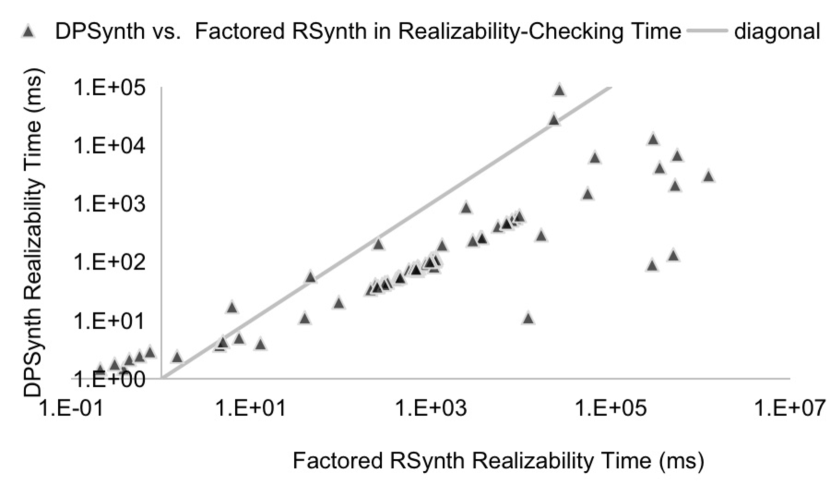
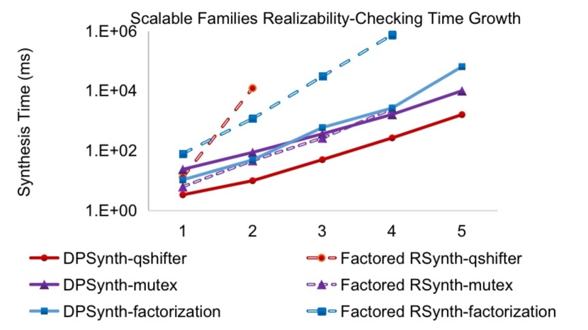
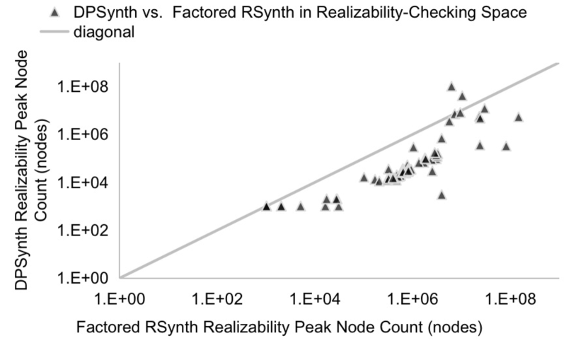
Figure 2(a) shows overall running-time comparison between DPSynth and Factored RSynth for realizability checking. A clear pattern that emerges is there is a difference in relative performance between very small problems (solvable within millisecond) and larger problems. DPSynth underperforms Factored RSynth on small instances, but outperforms on larger instances and the difference increases exponentially as input size grows. We conclude that planning overhead dominates on small input instances, but that effect fades off as instances get larger and the planning pays off. In memory usage comparison444The charts for space consumption for both phases are in the Appendix C. – using peak node count as a measurement – DPSynth uses less memory than Factored RSynth. Here the graded project-join-tree approach is advantageous, and planning incurs no overhead.
To evaluate scalability, we take the scalable benchmark families mentioned previously, and compare the logarithmic-scale slope in their running time as sizes of benchmarks increase. As indicated in Figure. 2(b), DPSynth scales exponentially better than Factored RSynth, as the planning overhead fades in significance as instances grow. We see a steeper slope on the exponential scale in DPSynth trends over factored RSynth. Some data points for larger benchmarks in the families (horizontal coordinates on chart) are missing because factored RSynth is not able to finish solving these instances in realizability-checking phase within the time limit.
5.2 Synthesis
The experiments on synthesis of witnesses answer the following research questions:
-
•
How does DPSynth compare in execution time to factored RSynth?
-
•
Does the influence of planning investment reduces as problem gets large?
-
•
What do we see in growth of tree widths and synthesis execution time?
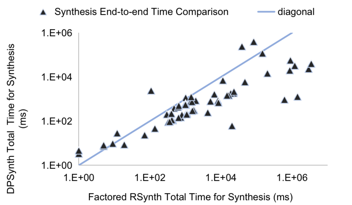
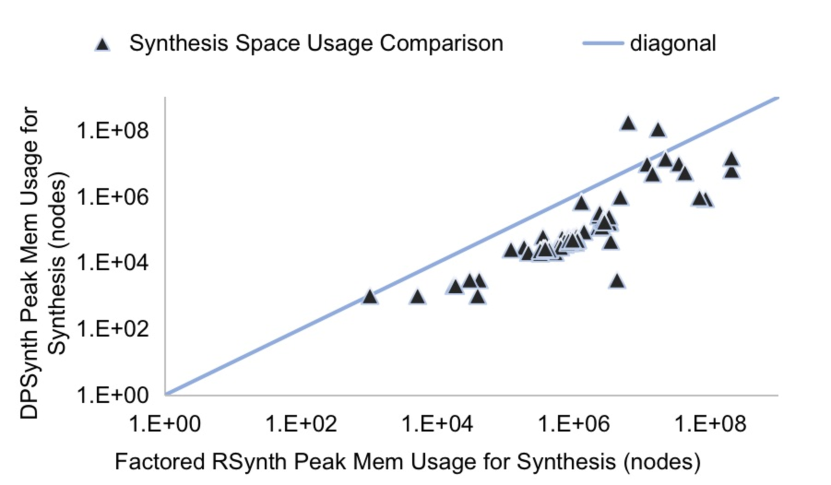
Using the same set of benchmarks and setting under the methodology as in Section 5.1, we applied our synthesis procedure to both fully realizable and partially realizable benchmarks. This broadens the scope of Boolean synthesis beyond that of fully realizable benchmarks, which is the scope of earlier work, as discussed above. Regarding end-to-end synthesis (planning, realizability checking, and synthesis, combined) DPSynth outperforms Factored RSynth in running time as illustrated in Figure 3(a). As with realizability checking, planning overhead dominates for small instances, as discussed in Section 3, but DPSynth solves large benchmarks faster and shows significant advantage as problem size increases, once the planning overhead fades in significance. In memory usage there is consistent relative performance of DPSynth vs. Factored RSynth.
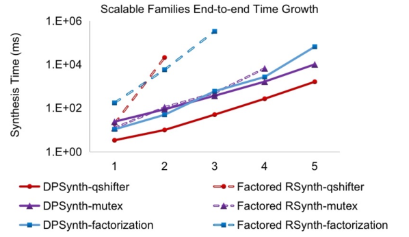
We again selected three scalable benchmark families, scaled based on a numerical parameter. As shown in Figure 3(b), DPSynth scales exponentially as benchmark size increases. Similarly to the case in realizability checking, the missing data points on larger benchmarks in the scalable families presented by the dashed lines are caused by the timeouts by factored RSynth.
While DPSynth shows performance advantage over Factored RSynth with respect to our benchmark suite, one cannot conclude that DPSynth always dominates Factored RSynth. This is because DPSynth involves computationally nontrivial planning phase, and it is not possible to say definitively that the planning overhead always pays off.
We can conclude, however, that DPSynth is an important addition to the portfolio of algorithms for boolean synthesis.
5.3 Tree Widths and Realizability
Graded project-join trees enable the computation of the realizability set in a way that minimizes the set of support of intermediate ADDs (Algebraic Decision Diagrams), saving time and memory. But computing these trees is a heavy computational task. In this section, we study the impact of tree width on realizability checking.
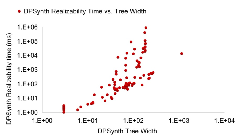
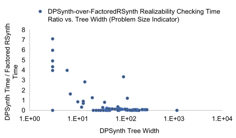
Figure 4(a) presents the range of realizability time run by DPSynth along increasing tree widths. As we see, increases in tree widths implies an increase in running time for realizability-checking. Figure 4(b), depicts the ratio of realizability time, computed by that of DPSynth over Factored RSynth, with respect to tree width, for problem instances that can be solved by both solvers. As treewidth increases, the over-performance of DPSynth over Factored RSynth increases, as planning overhead decreases in significance for higher-treewidth instances.
Synthesis execution time has similar relation with tree widths.
5.4 Comparison with Non-BDD-Based Synthesis
To complement out evaluation, we include additional experiments to verify whether DPSynth is competitive with non-BDD-based synthesis solvers, as motivated in Section 1. We compare with Manthan [17], a leading tool that is not based on decision diagrams, and find that DPSynth performs favorably.
We present a general picture by the following table, which shows the overall strength of the dynamic-programming decision-diagram approach, by measuring the time and space usage of experiments on the dataset selected from QBFEVAL’16 to QBFEVAL’19. DPSynth and Manthan each is able to solve some benchmarks that the other does not solve.
In order to compare the running time, we compare against Manthan using the DPSynth end-to-end synthesis time, which is the sum of tree-decomposition time, compilation, realizability-checking time, and synthesis time.
As the overall picture of synthesis solving, DPSynth shows a better time performance on most instances. DPSynth and Manthan each has strength on some instances, but the number of benchmarks that only DPSynth solves is larger than those solved only by Manthan. On those that are solved by both, DPSynth takes less time in most of them. See Appendix D for more illustrative data on specific fully and partially-realizable benchmarks.
| Number of benchmarks | |
|---|---|
| solved by Manthan | 79 |
| solved by DPSynth | 102 |
| solved by both Manthan and DPSynth | 70 |
| solved by Manthan but not by DPSynth | 9 |
| solved by DPSynth but not by Manthan | 32 |
6 Concluding Remarks
To summarize the contribution in this work, we propose a novel symbolic dynamic programming approach for realizability checking and witness construction in boolean synthesis, based on graded project-join trees. The algorithm we propose here combine a bottom-up realizability-checking phase with a top-down synthesis phase. We demonstrated experimentally that our approach, implemented in the DPSynth tool, is powerful and more scalable than the approach based on CSP heuristics (Factored RSynth). Another crucial contribution of this work is the inclusion of partial realizability checking, which applies to 30% of the total number of benchmarks. As we explain in introduction, this consideration is motivated by the need in modular circuit design and temporal synthesis to locate the scope of realizable inputs in iterative constructions.
There are many directions for future work. Variable ordering is a critical issue in decision-diagram algorithms, and should be explored further in the context of our approach. In particular, dynamic variable ordering should be investigated [25]. Also, in our work here we used high-level API of the BDD package CUDD, but it is possible that performance gains can be obtained by using also low-level BDD-manipulating APIs. The question of how to provide certificates of unrealizability also needs to be explored, c.f., [9, 8].
As mentioned earlier, quantifier elimination is a fundamental algorithmic component in temporal synthesis [30]. Tabajara and Vardi explored a factored approach for temporal synthesis [28]. It would be worthwhile to explore also the graded project-tree approach for boolean synthesis in the context of factored temporal synthesis. Finally, quantifier elimination is also a fundamental operation in symbolic model checking [11] and partitioning techniques have been explored in that context [10]. Therefore, exploring the applicability of our dynamic-programming approach in that setting is also a promising research direction.
6.0.1 Acknowledgements
This work was supported in part by NSF grants IIS-1527668, CCF-1704883, IIS-1830549, CNS-2016656, DoD MURI grant N00014-20-1-2787, an award from the Maryland Procurement Office, the Big-Data Private-Cloud Research Cyberinfrastructure MRI-award funded by NSF under grant CNS-1338099 and by Rice University’s Center for Research Computing (CRC).
References
- [1] Akshay, S., Arora, J., Chakraborty, S., Krishna, S., Raghunathan, D., Shah, S.: Knowledge compilation for boolean functional synthesis. In: 2019 Formal Methods in Computer Aided Design (FMCAD). pp. 161–169. IEEE (2019)
- [2] Akshay, S., Chakraborty, S., Goel, S., Kulal, S., Shah, S.: What’s hard about boolean functional synthesis? In: Chockler, H., Weissenbacher, G. (eds.) Computer Aided Verification - 30th International Conference, CAV 2018, Held as Part of the Federated Logic Conference, FloC 2018, Oxford, UK, July 14-17, 2018, Proceedings, Part I. Lecture Notes in Computer Science, vol. 10981, pp. 251–269. Springer (2018)
- [3] Akshay, S., Chakraborty, S., Goel, S., Kulal, S., Shah, S.: Boolean functional synthesis: hardness and practical algorithms. Formal Methods in System Design 57(1), 53–86 (2021)
- [4] Bahar, R.I., Frohm, E.A., Gaona, C.M., Hachtel, G.D., Macii, E., Pardo, A., Somenzi, F.: Algebric decision diagrams and their applications. Formal methods in system design 10(2), 171–206 (1997)
- [5] Bellman, R.: Dynamic programming. Science 153(3731), 34–37 (1966)
- [6] Bodlaender, H.L., Bonnet, É., Jaffke, L., Knop, D., Lima, P.T., Milanič, M., Ordyniak, S., Pandey, S., Suchỳ, O.: Treewidth is np-complete on cubic graphs (and related results). arXiv preprint arXiv:2301.10031 (2023)
- [7] Bryant, R.E.: Graph-based algorithms for Boolean function manipulation. IEEE TC 100(8), 677–691 (1986)
- [8] Bryant, R.E., Heule, M.J.: Dual proof generation for quantified boolean formulas with a bdd-based solver. In: CADE. pp. 433–449 (2021)
- [9] Bryant, R.E., Heule, M.J.: Generating extended resolution proofs with a bdd-based sat solver. In: International Conference on Tools and Algorithms for the Construction and Analysis of Systems. pp. 76–93. Springer (2021)
- [10] Burch, J.R., Clarke, E.M., Long, D.E.: Symbolic model checking with partitioned transistion relations. In: Proc. IFIP 10.5 Int’l Conference on Very Large Scale Integration. IFIP Transactions, vol. A-1, pp. 49–58. North-Holland (1991)
- [11] Burch, J.R., Clarke, E.M., McMillan, K.L., Dill, D.L., Hwang, L.J.: Symbolic model checking: 1020 states and beyond. Information and computation 98(2), 142–170 (1992)
- [12] Dudek, J.M., Phan, V.H.N., Vardi, M.Y.: DPMC: weighted model counting by dynamic programming on project-join trees. In: Proc. 26 Int’l Conf. on Principles and Practice of Constraint Programming. Lecture Notes in Computer Science, vol. 12333, pp. 211–230. Springer (2020)
- [13] Dudek, J.M., Phan, V.H.N., Vardi, M.Y.: Procount: Weighted projected model counting with graded project-join trees. In: Li, C., Manyà, F. (eds.) Theory and Applications of Satisfiability Testing - SAT 2021 - 24th International Conference, Barcelona, Spain, July 5-9, 2021, Proceedings. Lecture Notes in Computer Science, vol. 12831, pp. 152–170. Springer (2021)
- [14] Dudek, J.M., Phan, V.H., Vardi, M.Y.: ADDMC: weighted model counting with algebraic decision diagrams. In: AAAI. vol. 34, pp. 1468–1476 (2020)
- [15] Fried, D., Tabajara, L.M., Vardi, M.Y.: BDD-based Boolean functional synthesis. In: Proc. 28th Int’l Conf. on Computer Aided Verification. Part II. Lecture Notes in Computer Science, vol. 9780, pp. 402–421. Springer (2016)
- [16] Gogate, V., Dechter, R.: A complete anytime algorithm for treewidth. arXiv preprint arXiv:1207.4109 (2012)
- [17] Golia, P., Roy, S., Meel, K.S.: Manthan: A data-driven approach for boolean function synthesis. In: International Conference on Computer Aided Verification. pp. 611–633. Springer (2020)
- [18] Golia, P., Slivovsky, F., Roy, S., Meel, K.S.: Engineering an efficient boolean functional synthesis engine. In: 2021 IEEE/ACM International Conference On Computer Aided Design (ICCAD). pp. 1–9. IEEE (2021)
- [19] Hachtel, G.D., Somenzi, F.: Logic synthesis and verification algorithms. Springer Science & Business Media (2007)
- [20] Hamann, M., Strasser, B.: Graph bisection with pareto-optimization. In: Goodrich, M.T., Mitzenmacher, M. (eds.) Proceedings of the Eighteenth Workshop on Algorithm Engineering and Experiments, ALENEX 2016, Arlington, Virginia, USA, January 10, 2016. pp. 90–102. SIAM (2016)
- [21] Moskewicz, M.W., Madigan, C.F., Zhao, Y., Zhang, L., Malik, S.: Chaff: Engineering an efficient sat solver. In: Proceedings of the 38th annual Design Automation Conference. pp. 530–535 (2001)
- [22] Narizzano, M., Pulina, L., Tacchella, A.: The QBFEVAL web portal. In: Proc. 10th European Conf. on Logics in Artificial Intelligence. Lecture Notes in Computer Science, vol. 4160, pp. 494–497. Springer (2006)
- [23] Rabe, M.N., Seshia, S.A.: Incremental determinization. In: Creignou, N., Berre, D.L. (eds.) Theory and Applications of Satisfiability Testing - SAT 2016 - 19th International Conference, Bordeaux, France, July 5-8, 2016, Proceedings. Lecture Notes in Computer Science, vol. 9710, pp. 375–392. Springer (2016)
- [24] Robertson, N., Seymour, P.D.: Graph minors. x. obstructions to tree-decomposition. Journal of Combinatorial Theory, Series B 52(2), 153–190 (1991)
- [25] Rudell, R.: Dynamic variable ordering for ordered binary decision diagrams. In: Proceedings of 1993 International Conference on Computer Aided Design (ICCAD). pp. 42–47. IEEE (1993)
- [26] Somenzi, F.: CUDD: CU Decision Diagram Package Release 3.0.0. University of Colorado at Boulder (2015)
- [27] Tabajara, L.M., Vardi, M.Y.: Factored boolean functional synthesis. In: Stewart, D., Weissenbacher, G. (eds.) 2017 Formal Methods in Computer Aided Design, FMCAD 2017, Vienna, Austria, October 2-6, 2017. pp. 124–131. IEEE (2017)
- [28] Tabajara, L.M., Vardi, M.Y.: Partitioning techniques in ltlf synthesis. In: Int’l Joint Conference on Artificial Intelligence (2019)
- [29] Zhu, S., Tabajara, L.M., Li, J., Pu, G., Vardi, M.Y.: A symbolic approach to safety ltl synthesis. In: Proc. 13th Int’l Haifa Verification Conference. Lecture Notes in Computer Science, vol. 10629, pp. 147–162. Springer (2017)
- [30] Zhu, S., Tabajara, L.M., Li, J., Pu, G., Vardi, M.Y.: Symbolic ltlf synthesis. In: Proc. 26th Int’l Joint Conference on Artificial Intelligence. pp. 1362–1369. ijcai.org (2017)
Appendix 0.A Proofs
0.A.1 Proof of Theorem. 3.1
Proof.
We first prove the correctness of post-valuations computed. Case 1: If is a leaf in , , the returned encodes in line 5, which is the clause represented by . This is the same BDD as in Definition 6.
Case 2: Otherwise, we just need to show in the loop in line 9-12, BDD is always equivalent to the conjunction . As in Def. 6, we denote the represented boolean formula of BDD by . We use induction and assume that by the end of every iteration, , where is the set of all children nodes that have been traversed by the end of the last iteration. In the base case, , where is the first children node traversed. Hence it is returns as defined. Specifically, if , then the iteration is the last iteration since conjunction of boolean formulas with is also .
Next we prove the induction step. If in the new iteration the BDD is not , then it is updated to the conjunction of , exactly matching the inductive hypothesis. So this invariant is preserved in this new iteration. If in the new iteration of , the BDD encodes , the conjunction in Def. 6 is also , so the pre-valuation line 12 is consistent with the inductive hypothesis. Hence by the end of every iteration of the loop in lines 9-12, we have the invariant that . Line 13 performs the operation of existential quantification in Def. 6. Hence we have the correctness of Alg. 1.
Next we show the equivalence between the returned pre-valuations and its definition. For leave nodes , the pre-valuation computed in line 4 corresponds to Definition. 6. In the case of internal node, is returned either by the end of the for-loop in lines 9-12, or returned whenever it is equal to . We also know that is proved above to be equivalent to its definition, and the fact that a conjunction with zero is always 0, in the sense of both boolean formulas and BDDs. Therefore we are only left to show that the pre-valuation defined in Definition. 6 is equivalent to at the end of Algorithm. 1. Since is updated in line 10 only, it is equivalent to the conjunction of and for all , which is exactly as defined in its Definition. 6. Hence we complete the proof.
∎
0.A.2 Proof of Theorem. 3.3
Proof.
First, we prove the first statement of Theorem 3.3. Suppose , i.e., there is full realizability. We need to show that throughout the for-loop in lines 10-16. i.e., We need to prove that in all iterations, the algorithm never goes to line 14. That is, to show that for all . By Definition 6 and Theorem 3.1, the post-valuation of internal nodes is equal to the conjunction of post-valuations under it with its labelled variables existentially quantified. This is then equivalent to the conjunctions of all leaves in its descendants, projecting out all variables labelled in its descendants. Since we assume full realizability, all clauses represented by the leaves are satisfiable, and thus the post-valuations of all the internal nodes are equal to , not to mention the visited internal nodes in the uppermost level of .
To prove the other direction, assume that Algorithm 2 returns fully realizable. Then line 17 must confirms, and it is equivalent to say is always . Then for all internal nodes in , post-valuation is . Since all the leaves in the original graded project-join tree has one and only one ancestor in , the conjunction of the post-valuations of all is equivalent to and to . Hence achieves full realizability.
Next, we prove that a returned not realizable from Algorithm 2 is sufficient condition for null realizability of . Suppose Algorithm 2 returns not realizable. Then in line 11, . There is some internal node without parents in , such that its post-valuation in is the -BDD. Hence, by Def. 6, the conjunction of post-valuations of its children node in is . Thus there does not exist variables labelled by this node , such that the conjunction of clauses in its descendants is satisfiable. Thus, there does not exist a set of boolean values for all the variables, that satisfies the conjunction of clauses in descendants of . Moreover, the conjunction of all clauses in is not satisfiable. Thus, does not achieve partial realizability in its domain and null realizability is proved.
Hence we complete the proof for Theorem 3.3.
∎
0.A.3 Proof of Theorem. 3.2
This theorem follows from the definition of realizability set and Definition. 6:
Proof.
Let be a graded project-join tree of CNF . Let be the set of highest nodes. Denote descendants of node by .
From Definition. 6,
where . Then the realizability set is defined to be
We also know that each variable is labelled under one and only one highest level node, by definition of a graded project-join tree. Hence
Therefore, the conjunction of pre-valuations for all , i.e., , we can show:
| (by definition of graded project-join tree) | ||||
Theorem 3.2 is proved. ∎
0.A.4 Proof of Theorem. 3.4
Proof.
Suppose Algorithm 3 returns not realizable. Then the post-valuation of the root is -BDD. By Definition 6, it is either a leave representing an unsatisfiable clause, or the variables do not satisfy the conjunction of all clauses in the tree. In the trivial former case it is obviously not realizable.
In the latter case, since is the output of Algorithm 2 where all internal nodes are eliminated, the post-valuation of these new leaves remain the same in the updated tree . Taking existential projections on an output variable only to the clauses where it has occurrences in, is logically equivalent to quantifying it on the entire formula. The same reasoning applied to their symbolic representations. Hence the conjunction of the clauses in with all variables quantified is logically equivalent to with all and existentially quantified. Hence, there do not exist and variables that satisfy . i.e., if Algorithm 3 returns not realizable, there is null realizability.
On the other hand, assume Algorithm 3 returns partially realizable. Then in line 1 is not -BDD. That is, the conjunction of leaves has satisfying set of variables labelled. By analysis above, it is equivalent to satisfiability of the CNF formula represented by the original tree in Algorithm 2. That is, there is partial realizability. Since null and partial realizability is complementary to each other, we do not need to prove the reverse directions in both cases. Hence the correctness of Theorem 3.4 is proved. ∎
0.A.5 Proof of Lemma. 3
Proof.
From the definition of of project-join tree, if then every clause where appears must be in a leaf node that descends from . Since is not a descendant of , then either no clauses containing have been joined on the way to form , or (if is a descendant of instead) has already been existentially quantified. ∎
0.A.6 Proof of Theorem. 4.1
Proof.
We use to denote the set of children of node , the set of descendants of node (not including itself), and the set of descendants of that are leaves. We also use the notation for the set of variables synthesized in node and for the set of variables synthesized in nodes that are descendants of . Finally, we denote by the witness for variable after all witnesses synthesized in or its descendants have been substituted into it. Note that if where is not a descendant of (including when ) then (by Lemma 3).
Assume that, for an arbitrary node , returns a correct witness for every . In other words, that . Recall that both and can still be dependent not only on the variables, but also on the variables of nodes that descends from (but no other nodes, as per Lemma 3).
We show by induction that the following holds for every node :
This expression states that are witnesses for (note that these witnesses might still depend on variables from ancestors of ). If is the root of the tree, then and , and so . In other words, are witnesses for the variables. Note that the are equivalent to the final witnesses returned in line 4. Therefore, the witnesses returned by Algorithm 4 are correct. All that is left is to prove (0.A.6).
Base case.
Assume is a leaf. In that case, , and are all empty, and . Therefore, (0.A.6) holds vacuously.
Inductive step.
Assume is an internal node, and (0.A.6) holds for all of ’s children . We will show that it holds for as well. Note that we use the fact that, by early quantification, .
| (and by ) | ||||
| (by induction hypothesis) | ||||
| (since the are disjoint) | ||||
| (*) | ||||
| (since ) | ||||
| (since ) | ||||
The step marked with (* ‣ 0.A.6) above merits a more detailed explanation. In the step before, the substitution is performed at the end, and therefore this substitution also affects the witnesses from the child nodes (which might depend on the variables ). When we move this substitution to the beginning, to ensure equivalence we must also substitute into the substitutions , which updates to . ∎
Appendix 0.B Synthesis in Factored RSynth
Let (each is a factor, for example a clause or a cluster). We associate with the factor the set of the output variables that occur in but do not occur in a factor with . Equivalently speaking, the set consists of the variables from that only occur in factors . Moreover, since each includes all variables that satisfy this criterion, for all , if a variable , then it is guaranteed that for .
The intuition behind this definition is that an output variable does not depend on the formulas . Thus, these clauses can be ignored when constructing a witness for . i.e., the values of clauses in these other factors do not affect the function constructed for this variable. We use the notation to denote the BDD representing the factor , and to denote the existential quantification of all variables as a block. We can then compute realizability by using early quantification:
Note that, from the correctness of early quantification, we have that . Like before, is equivalent to the realizability set . Note that this framework already has some kind of tree structure. Each corresponds to a leaf, and each corresponds to an internal node, with children and , and labeled by . is the root of the tree. Similarly to how realizability was computed inside-out in the monolithic case, in this case realizability is computed bottom-up, from the leaves to the root. Witness construction, which was computed outside-in in the monolithic case, is in this case computed top-down, from the root to the leaves (witnesses in a single node can be computed as in the monolithic procedure):
| For all , is computed from | ||
| For all , is computed from | ||
| For all , is computed from | ||
| For all , is computed from | ||
| For all , is computed from | ||
Note that, similarly to how in the monolithic case each witness depends on the witnesses of the previous variables, in the factored case the witnesses of a child depend on the witnesses of its ancestors. Parent nodes propagate witnesses to their children, who then substitute them into before computing witnesses for their own variables. These witnesses are then propagated to their own children. Note that corresponds to the pre-valuation from Definition 6.
Appendix 0.C Space Performance Charts
Appendix 0.D DPSynth vs. Manthan
We measure the time and space usage of experiments on the dataset selected from QBFEVAL’16 to QBFEVAL’19. DPSynth and Manthan [17] each solves for some benchmarks that the other does not solve.
As the overall picture of synthesis solving, DPSynth and Manthan each has strength on some instances, but the number of benchmarks that only DPSynth solves is larger than those solved only by Manthan. On the intersection of solved sets, DPSynth takes less time usage.
Overall, DPSynth shows a better time performance. In order to compare the running time, we compare against Manthan using the DPSynth end-to-end synthesis time, which is the sum of tree-decomposition time, compilation, realizability-checking time, and synthesis time. For partially realizable instances, since Manthan returns UNSAT for partially realizable benchmarks, we compare with Manthan by measuring the realizability time of DPSynth, which is the sum of tree-decomposition, compilation and realizability-checking time. This is illustrated in the table presented in Section 5 of formal text.
The results show a better performance in DPSynth running time, in both fully and partially realizable cases. This shows the strength of the dynamic-programming decision-diagram approach.
| Benchmark | Manthan time (s) | DPSynth time (s) | Manthan / DPSynth time |
|---|---|---|---|
| mutex-2-s | 26.62365198 | 0.017328861 | 1536.376337 |
| mutex-4-s | 70.10412574 | 0.057425382 | 1220.786407 |
| qshifter_3 | 0.02080822 | 0.004227581 | 4.922015666 |
| qshifter_4 | 0.035684586 | 0.011800355 | 3.024026444 |
| qshifter_5 | 0.118482351 | 0.056386868 | 2.101240156 |
| qshifter_6 | 0.548010349 | 0.290776052 | 1.884647465 |
| qshifter_7 | 3.304552555 | 1.692991177 | 1.951901817 |
| stmt1_145_146 | 1.481198549 | 0.007940356 | 186.5405719 |
| stmt1_20_21 | 1.161505938 | 0.005571153 | 208.4857367 |
| stmt1_60_61 | 138.0251365 | 1.923284128 | 71.7653385 |
| stmt1_629_630 | 60.86966228 | 0.820687097 | 74.16914742 |
| stmt1_787_788 | 92.2114253 | 1.340908081 | 68.76789439 |
| stmt1_811_812 | 5.000648737 | 0.042724069 | 117.045236 |
| stmt1_919_920 | 16.3737123 | 0.216405419 | 75.6622102 |
| stmt11_643_645 | 13.83426762 | 0.148434139 | 93.20138689 |
| stmt124_966_965 | 17.15093589 | 0.226107464 | 75.8530284 |
| stmt16_0_1 | 0.078123331 | 0.021049437 | 3.711421406 |
| stmt16_285_286 | 12.3903234 | 0.199766912 | 62.02390214 |
| stmt16_47_48 | 127.7006507 | 1.851167077 | 68.98386012 |
| stmt16_818_819 | 8.039676428 | 0.099669646 | 80.66323851 |
| stmt16_950_951 | 21.96217847 | 0.321454774 | 68.32120797 |
| stmt17_99_98 | 147.940861 | 2.241282086 | 66.00724733 |
| stmt18_258_260 | 9.160577059 | 0.098143359 | 93.33873583 |
| stmt2_480_551 | 16.77611017 | 0.226805481 | 73.9669522 |
| stmt2_649_647 | 11.21149755 | 0.139258954 | 80.50827055 |
| stmt2_649_723 | 11.58830237 | 0.14303965 | 81.01461639 |
| stmt2_649_776 | 14.4783535 | 0.196231457 | 73.7820211 |
| stmt21_326_327 | 22.5036993 | 0.357303104 | 62.98209853 |
| stmt24_148_149 | 1.197834015 | 0.006430307 | 186.2794443 |
| stmt24_292_293 | 9.379323483 | 0.109969875 | 85.28993493 |
| stmt24_7_8 | 0.017041206 | 0.001758292 | 9.691909171 |
| stmt24_765_766 | 18.09966111 | 0.220442702 | 82.10596653 |
| stmt27_296_297 | 10.50176525 | 0.115043276 | 91.28534597 |
| stmt27_946_955 | 20.3260808 | 0.247080786 | 82.26491881 |
| stmt3_639_640 | 8.168511868 | 0.079512754 | 102.7320959 |
| Benchmark | Manthan time (s) | DPSynth time (s) | Manthan / DPSynth time |
|---|---|---|---|
| stmt32_570_572 | 23.86345649 | 0.32441781 | 73.55778799 |
| stmt37_941_942 | 129.7759182 | 1.517532121 | 85.51774058 |
| stmt38_943_942 | 117.9836717 | 1.531322152 | 77.04693066 |
| stmt41_118_131 | 9.311798096 | 0.22846856 | 40.75745956 |
| stmt41_566_580 | 44.67906404 | 0.83791215 | 53.32189542 |
| stmt41_738_737 | 17.30380273 | 0.214580042 | 80.64031756 |
| stmt41_738_749 | 36.58995533 | 0.674991152 | 54.2080518 |
| stmt44_435_436 | 12.76951456 | 0.144744236 | 88.22123018 |
| stmt44_554_555 | 22.60296774 | 0.29673466 | 76.17232088 |
| stmt44_554_604 | 23.51070952 | 0.307722947 | 76.40219799 |
| stmt44_916_917 | 16.47536898 | 0.19140868 | 86.07430434 |
| stmt7_33_34 | 14.49155951 | 0.934846089 | 15.50154584 |
| stmt70_191_213 | 8.378497839 | 0.09022127 | 92.86610396 |
| stmt70_495_501 | 22.71755934 | 0.314747484 | 72.1770959 |
| stmt70_854_859 | 16.48648357 | 0.203281798 | 81.10162216 |
| stmt72_696_721 | 17.04460955 | 0.204169481 | 83.4826511 |
| stmt82_224_225 | 10.50310063 | 0.105692302 | 99.37431994 |
| stmt86_889_890 | 21.63464522 | 0.284072161 | 76.15897717 |
| stmt9_350_351 | 8.726649284 | 0.092352257 | 94.49308082 |
| subtraction32 | 3.983768463 | 285.7623599 | 0.013940844 |
| tree-exa10-10 | 0.580000877 | 0.001643786 | 352.8445171 |
| tree-exa10-15 | 0.744118929 | 0.002058999 | 361.3983926 |
| tree-exa10-20 | 0.94502902 | 0.002538212 | 372.3207598 |
| tree-exa10-25 | 1.136503696 | 0.002991756 | 379.8784715 |
| tree-exa10-30 | 1.398799896 | 0.00363048 | 385.2933761 |
| factorization8 | 26.02147222 | 0.01355423 | 1919.804534 |
| rankfunc37_signed_16 | 2.976966858 | 0.020192158 | 147.4318326 |
| stmt137_903_911 | 18.31892133 | 0.2235378 | 81.94999382 |
| stmt19_3_214 | 67.52295566 | 970.6645171 | 0.069563639 |
| stmt19_66_214 | 84.54595137 | 148.8763251 | 0.567893863 |
| stmt2_976_999 | 3228.63344 | 57.85746008 | 55.80323498 |
| stmt21_5_134 | 47.65692377 | 14.28987617 | 3.335013067 |
| stmt21_84_215 | 88.41444421 | 135.9611531 | 0.650291956 |
| stmt27_16_97 | 53.51791215 | 9.510231213 | 5.627403893 |
| stmt27_584_603 | 24.56984329 | 0.329176383 | 74.64035867 |