Sensitivity Analysis for Active Sampling, with Applications to the Simulation of Analog Circuits

Abstract

We propose an active sampling flow, with the use-case of simulating the impact of combined variations on analog circuits. In such a context, given the large number of parameters, it is difficult to fit a surrogate model and to efficiently explore the space of design features. By combining a drastic dimension reduction using sensitivity analysis and Bayesian surrogate modeling, we obtain a flexible active sampling flow. On synthetic and real datasets, this flow outperforms the usual Monte-Carlo sampling which often forms the foundation of design space exploration.

I Introduction

I-A Context and literature

Context: Performances of integrated circuit are knowingly sensitive to a plurality of effects linked to the fabrication process or electrical stress via their impact on each device’s characteristics (process and mismatch variations, temperature, voltage, aging, etc). As such, today’s analog design flows are proposing various tools to simulate the impact of these effects. This has conducted the design flow to usually focus first on the impact of statistical variations of devices on the circuit performances using dedicated tools, and then once the circuit is tuned with respect to these, a next step can be to evaluate aging with other tools to verify that the impact of degraded devices stays within the remaining performance margins left after statistical simulation. If this sequential approach may be fine for circuits designed with mature nodes where aging’s impact on devices is normally orders of magnitude less compared to statistical variations, this becomes impractical in advanced nodes where it not rare to see the impact of aging more comparable to the one of statistical variations, as for instance mentioned in [1]. In such cases, the only way would be to simulate the combined effect of these different causes, which leads to an explosion in number of simulations to run if for example at each statistical variations sample we execute the often multi-step stress conditions execution to add aging degradation. Methods helping to reduce the total number of simulations in such multi-variation domains scenarios are therefore highly desired to limit the exploding CPU cost they imply.

Indeed, Monte Carlo (MC) based analysis is necessary to provide a robust estimation assessment of the circuit’s design performance due to fabrication process variations. MC consists in the standard approach for routine design validation [2]. On the other hand, MC based analysis requires a large number of computationally expensive circuit simulations, making it unfeasible for modern and more complex circuit technologies. To overcome this limitation, Importance sampling (IS) methods [2, 3] can be used instead to draw samples from artificially modified distributions shifted to the targeted operating zones of interest, normally towards fail regions. Thus, the convergence of the estimated robustness assessment can be accelerated since the ”rare” events are prone to be drawn around these targeted regions of interest. The downside is that these methods normally favor limited specific zones of interest, therefore disfavoring the exploration and discovery of other important operating zones that end up being ignored [4].

Surrogate Modeling: Still to avoid the large number of expensive circuit simulations, data-driven surrogate models [4] can be constructed and used to approximate the circuit’s response. Thanks to that, the circuit’s design performance can be assessed in a faster manner. However, the main disadvantage is that these models require sufficient training samples, i.e., samples that are representative of the circuit performance dispersion. Moreover, the data-driven surrogate models suffer from the “curse of dimensionality” [4, 5]. More specifically, the high dimensionality (which is quite common in modern analog circuits) makes it challenging to train the surrogate models.

Fortunately, some previous research [6] indicates that not all variations in input parameters are equally important. In reality, any given circuit performance measure is normally dominated by a group of critical devices, whereas the other devices have very little to no influence, especially in the case where the circuit has a symmetric design intended to alleviate the process variation [4].

Active Learning: This knowledge allows to consider “dimension reduction” capable to reduce the input dimension such that only the key and relevant parameters are isolated. One possibility is to combine the efficiency of faster evaluations of surrogate models with active learning to sequentially reduce the prediction error [5]. [7] adopts a Gaussian process (GP) to approximate the underlying circuit performance function and an entropy reduction criteria for active learning. One limitation is that entropy-based criterion is known for being computationally expensive. [4] adds a nonlinear-correlated deep kernel method with feature selection to isolate the key determinant features to focus on and to consider in the surrogate modeling approach that also uses a GP. These previously proposed approaches have been assessed to tackle up to 1k input dimensions, which can be considered a ”small” analog circuit. A robust feature selection method is thus necessary to allow the use of surrogate modeling approaches in this application.

Goals and contributions: Having at our disposal an analog circuit simulator, we aim for an efficient exploration of the parameter space in order to limit the number of samples to effectively simulate. To that end, the corner stones of our method will be the tools of dimensionality reduction on the one hand, and surrogate modeling on the other hand.

I-B Description of Sampling Flow

Within the context of integrated circuit design, the effects mentioned in Introduction are modelled by a random vector $X=\left(X^{(1)},\dots,X^{(D)}\right)$, where each $X^{(i)},\ i=1,\ldots,D$ is a real bounded random variable valued in $B^{(i)}$. These random variables are also called explanatory variables and $D$ is supposed to be very large. The performance of an integrated circuit is described by a random variable $Y=F(X)$, where the function $F$ is not easily accessible in practice. The function $F$ describes namely an expensive simulation and it is referred to as the ”black-box” or the ”computer code”. Here, we shall suppose that $F:B\rightarrow{\mathbb{R}}$. Also, it will be convenient to designate, for any subset $I\subset\llbracket 1,D\rrbracket$, the associated product space as

$$B(I):=\prod_{i\in I}B^{(i)}\ .$$ (1)

Naturally $X\in B:=B(\llbracket 1,D\rrbracket)=\prod_{i=1}^{D}B^{(i)}$.

Figure 1: Diagram of our active sampling flow.

Let us now describe our active sampling flow, which is illustrated in Figure 1. We assume that we have a first batch of $N_{0}\in{\mathbb{N}}^{*}$ realizations

$${\mathcal{S}}_{N_{0}}:=\left\{\left(x_{j},y_{j}\right)\in B\times{\mathbb{R}},\ 1\leq j\leq N_{0}\right\}\ ,$$ (2)

of the random variables $\left(X,Y\right)$. The goal is to successively choose new samples, until we reached a final budget $N_{f}\in{\mathbb{N}}^{*}$, with the best characterization of circuit performance.

Surrogate modeling: Assuming we have chosen a set of samples ${\mathcal{S}}_{N}$ for $N_{0}\leq N<N_{f}$, we construct surrogate model of $F$, denoted $\widehat{{\mathcal{F}}}_{N}$ based on the observations ${\mathcal{S}}_{N}$. Then this surrogate model $\widehat{{\mathcal{F}}}_{N}$, is used in order to choose the next sample point in $B$ for which the prediction through $\widehat{{\mathcal{F}}}_{N}$ is the most uncertain.

Among the multiple possibilities of surrogate models, we have opted for Gaussian Processes (GPs) [8], for their flexibility and because of their natural Bayesian framework. Indeed, given a GP $\widehat{{\mathcal{F}}}_{N}$, that has been trained to interpolate between the values of ${\mathcal{S}}_{N}$, we have access to both predictions on the entire space

$$\widehat{m}_{N}:x\mapsto{\mathbb{E}}\left[\widehat{{\mathcal{F}}}_{N}(x)\right]\ ,$$ (3)

and well as the variance

$$\widehat{v}_{N}:x\mapsto\operatorname{Var}\left[\widehat{{\mathcal{F}}}_{N}(x)\right]\ .$$ (4)

Dimensionality reduction: It is well known that GPs do not scale with the dimension. Therefore, it is absolutely necessary to identify $d\ll D$ relevant indices $I_{d}=\left(i_{1},\dots i_{d}\right)\subset\llbracket 1,D\rrbracket$ which better represent the variations at hand. Accordingly the trained Gaussian Process Regressor $\widehat{{\mathcal{F}}}_{N}$ is taken as a (random) map defined over $B(I_{d})$. Likewise for $\widehat{m}_{N}$ and $\widehat{v}_{N}$.

The statistical procedure for finding $I_{d}$ is the Feature Selection Algorithm 2, which is detailed in Section III along with the necessary statistical theory.

Optimized sampling: Thus we can choose the next sample $\widetilde{x}_{N+1}\in B(I_{d})$ as the one maximizing the variance, meaning that

$$\widetilde{x}_{N+1}=\left(\widetilde{x}_{N+1}^{(1)},\dots,\widetilde{x}_{N+1}^{(d)}\right)=\underset{x\in B(I_{d})}{\operatorname{argmax}}\ \widehat{v}_{N}(x)\ ,$$ (5)

which we depict in Algorithm 1.

0:   ${\mathcal{S}}_{N}$ : the training dataset of size $N$;

          $I_{d}=\left(i_{1},\dots,i_{d}\right)$ : labels of relevant features;

          $m$ : the number of candidate points ;

   $\widehat{{\mathcal{F}}}_{N}\leftarrow$ Gaussian Process Regressor trained on ${\mathcal{S}}_{N}$ ;

   ${\mathcal{S}}\leftarrow$ Sample $m$ i.i.d. points in $B(I_{d})$ according to the law of $\left(X^{(i)},i\in I_{d}\right)$ ;

  $\widetilde{x}_{N+1}\leftarrow$ Point in ${\mathcal{S}}$ maximizing variance (Eq. (5)) ;

  return  $\widetilde{x}_{N+1}=\left(\widetilde{x}_{N+1}^{(1)},\dots,\widetilde{x}_{N+1}^{(d)}\right)$

Algorithm 1 Optimized Sampling

In order to obtain a sample $x_{N+1}\in B$, it only remains to sample the remaining (non-relevant) coordinates $z_{N+1}\in~{}B(\llbracket 1,D\rrbracket\backslash I_{d})$. Then the new sample is obtained by concatenation $x_{N+1}:=(\widetilde{x}_{N+1},z_{N+1})\in B$. The associated output is obtained by invoking the black-box function $F$ to compute $y_{N+1}=F\left(x_{N+1}\right)$ and finally obtain ${\mathcal{S}}_{N+1}:={\mathcal{S}}_{N}\cup\left\{\left(x_{N+1},y_{N+1}\right)\right\}$ .

II Datasets

Dataset	Sample size	Outputs / dim $Y$	Attributes	Fictitious Attributes	Total Attributes (D)
$G_{\mathrm{Sobol^{\prime}}}^{(d=4)}$	$30\ 000$	$1$	$4$	$446$	$450$
HSOTA	$30\ 000$	$3$	$450$	$0$	$450$
$G_{\mathrm{Sobol^{\prime}}}^{(d=10)}$	$30\ 000$	$1$	$10$	$9\ 990$	$10\ 000$
FIRC	$9\ 982$	$2$	$44\ 959$	$0$	$44\ 959$

TABLE I: Characteristics of datasets. The Sobol’ $G$ function has extra noisy (fictitious) attributes added, in order to become comparable to the real datasets FIRC and HSOTA.

The datasets we use to showcase our active sampling flow are a standard Sobol G-function and simulations from actual analog circuits. Table I summarizes the content of this Section.

II-A The classical Sobol’ G-function

In the community of sensitivity analysis, it is common to use the following Sobol’ G-function for synthetic benchmarks [9]. Given $d\leq D$ and $a\in\left({\mathbb{R}}\backslash\{-1\}\right)^{d}$, such function $F=G_{\mathrm{Sobol^{\prime}}}^{(d)}$ is defined as

$$\begin{array}[]{ll}G_{\mathrm{Sobol^{\prime}}}^{(d)}:&[0,1]^{D}\rightarrow{\mathbb{R}}\\ &x\mapsto\prod_{i=1}^{d}\frac{|4x^{(i)}-2|+a_{i}}{1+a_{i}}\end{array}\ ,$$

which will be only considered for $a=0_{{\mathbb{R}}^{d}}$, meaning that

$$Y=G_{\mathrm{Sobol^{\prime}}}^{(d)}(X):=\prod_{i=1}^{d}|4X^{(i)}-2|\ .$$ (6)

The first $d$ variables, $(X^{(1)},\dots,X^{(d)})$, will be called the significant features, and the $D-d$ others, $(X^{(d+1)},\dots,X^{(D)})$, will be called the noisy features. We add these fictitious attributes to the dataset given by the Sobol’ G function, in order to artificially reproduce the same dimensionality found in the non-synthetic datasets (See Table I).

II-B Simulation of analog circuits

The analog circuits at hand are a High-Speed Operational Transconductance Amplifier (HSOTA) and a Fast Internal Reference Clock (FIRC) generator both designed in 16nm FinFET technology and composed each of few thousands of devices. See for example [10, 11] for general information about HSOTA amplifiers and clock circuits. We have at our disposal simulations performed thanks to SPICE-like analog simulators, which are industry standards. For example Cadence’s Spectre® Circuit Simulator [12]. Furthermore

• for the HSOTA device, the outputs are two slew rate measures (up and down) and an offset voltage, which all depend on $D=450$ explanatory variables ;

• for the FIRC device, the outputs are measures of the generated clock frequency and its duty cycle, which all depend on $D=44\ 959$ explanatory variables.

Notice that simulations take into account circuit aging, which depends on variables describing usage scenarios. Here, we do not include such aging variables, and by explanatory variables, we only mean process and mismatch variations, temperature and supply voltages in the design of circuits.

Of course, there is no intrinsic dimension $d$ in these cases. And naturally, the chosen dimensions depend on which output is considered. In practice, dimension reduction to the values $d_{HSOTA}\in\{10,13\}$ and $d_{FIRC}\in\{11,15\}$ is satisfactory.

III Features selection

III-A Chatterjee’s estimator of Cramèr-von-Mises indices

Our method for dimensionality reduction relies on the computation of sensitivity indices, which are powerful tools from the field of Global Sensitivity Analysis, as described in [13]. Thanks to such indices, one can assess, for $1\leq i\leq D$, how sensitive is $Y$ to a variable $X^{(i)}$. Throughout the paper, we will only consider the first order Cramèr-von-Mises indices (CvM indices) which are given by

$$\xi\left(X^{(i)},Y\right):=\frac{\int_{t\in{\mathbb{R}}}\operatorname{Var}\left[{\mathbb{E}}\left[\mathds{1}_{Y\leq t}\ |\ X^{(i)}\right]\right]{\mathbb{P}}_{Y}(dt)}{\int_{t\in{\mathbb{R}}}\operatorname{Var}\left[{\mathbb{P}}\left[Y\leq t\right]\right]{\mathbb{P}}_{Y}(dt)}\ .$$

When there is no ambiguity, we will note $\xi^{(i)}:=\xi\left(X^{(i)},Y\right)$ and we have that $\xi^{(i)}\in[0,1]$.

The remarkable property of the CvM index $\xi^{(i)}$ is that it vanishes if only if $Y$ and $X^{(i)}$ are independent. And it is equal to $1$ if and only if $Y$ is a function of $X^{(i)}$. As such, the CvM index $\xi^{(i)}$ quantifies the dependence, allowing us to decide whether or not the variable $X^{(i)}$ is relevant.

We will estimate these CvM indices empirically using Chatterjee’s method based on ranks. The estimator $\widehat{\xi}^{(i_{0})}_{N}$ is defined as follows. Given a feature $1\leq i_{0}\leq D$, let us assume that we have at our disposal $N\in{\mathbb{N}}^{*}$ i.i.d. realisations of $\left(X^{(i_{0})},Y\right)$

$${\mathcal{S}}_{N}^{(i_{0})}=\left\{\left(x_{j}^{(i_{0})},y_{j}\right)\in B^{(i_{0})}\times{\mathbb{R}},\ 1\leq j\leq N\right\}\ .$$

Let us sort the sample as $\left(x_{N,(j)}^{(i_{0})},y_{N,(j)}\right)_{1\leq j\leq N}$ such that

$$x_{N,(1)}^{(i_{0})}\leq\dots\leq x_{N,(N)}^{(i_{0})}\ .$$

Then we define this rank-based estimator for $\xi^{(i_{0})}$ by

$$\widehat{\xi}^{(i_{0})}_{N}:=1-\frac{3\sum_{j=1}^{N-1}\left|r_{j+1}-r_{j}\right|}{N^{2}-1}\ ,$$ (7)

where the ranks $r_{j}$’s are given by

$$\forall 1\leq j\leq N,\ r_{j}:=\sum_{k=1}^{N}\mathds{1}_{\left\{y_{N,(k)}\leq y_{N,(j)}\right\}}\ .$$

The almost sure convergence $\lim_{N\rightarrow\infty}\widehat{\xi}^{(i_{0})}_{N}=\xi^{(i_{0})}$ is given by [14, Theorem 1.1].

Thus, because of the simplicity of this estimator, it can be incorporated into a feature selection method as Algorithm 2.

0:  ${\mathcal{S}}_{N}$ : the training dataset of size $N$ ;

          $d\in{\mathbb{N}}^{*}$ : the number of features to select ;

  for $i\in\llbracket 1,D\rrbracket$ do

     Compute $\widehat{\xi}^{(i)}_{N}$ thanks to Equation (7);

  end for

  Take the $d$ features $\left(i_{1},\dots,i_{d}\right)$ maximizing $\left(\widehat{\xi}^{(i)}_{N}\right)_{1\leq i\leq D}$

  return  $\left(i_{1},\dots,i_{d}\right)$, most relevant $d$ feature labels

Algorithm 2 Feature Selection

III-B Conjecture for detection of noisy features

For statistically testing whether a fixed feature is relevant, we have at our disposal the following Central Limit Theorem for one estimator $\widehat{\xi}_{N}^{(i)}$.

Theorem III.1 (2.2 from [14]).

For all $1\leq i\leq D$, under the hypothesis

$$H_{0}^{(i)}:``X^{(i)}\ \mbox{is a noisy feature}^{\prime\prime}\ ,$$

the corresponding Chatterjee estimator, $\widehat{\xi}_{N}^{(i)}$, fluctuates according the following Central Limit Theorem (CLT)

$$\sqrt{N}\widehat{\xi}_{N}^{(i)}\rightarrow\mathcal{N}\left(0,\frac{2}{5}\right)\ .$$

However, for a feature selection with a high number of noisy variables, we need a joint test, in the sense that we need to test the following hypothesis

$$H_{0}=H_{0}^{(i_{1},\dots,i_{k})}:``X^{(i_{1})},\dots,X^{(i_{k})}\ \mbox{are the noisy features'' , }$$

where $(i_{1},\dots,i_{k})\in\mathcal{P}_{k}\left(\llbracket 1,D\rrbracket\right)$. In other words,

$$H_{0}=H_{0}^{(i_{1},\dots,i_{k})}=H_{0}^{(i_{1})}\cap\dots\cap H_{0}^{(i_{k})}\ .$$

Thus, under such $H_{0}$, it is natural to track the variable

$$\widehat{\xi}_{\mathrm{max}}=\widehat{\xi}_{\mathrm{max}}(N,\left(i_{1},\dots i_{k}\right)):=\max_{i\in\left(i_{1},\dots i_{k}\right)}\widehat{\xi}_{N}^{(i)}\ ,$$

given a sample size $N\in{\mathbb{N}}$. Notice that maxima of random variables are not always tractable. The case that is well studied is that of the maxima of independent variables with Gaussian tails. This is the topic of classical books such as [15]. In fact, under $H_{0}$, we expect the $\widehat{\xi}_{N}^{(i)}$ ’s to decorrelate from the samples of $Y$, so that $\widehat{\xi}_{\mathrm{max}}$ truly behaves like a maximum of i.i.d. random variables. Because Gaussian tails are a given thanks to the concentration inequalities in the proof of [14, Theorem 1.1], theorems describing extremal statistics such as [15, Theorem 1.5.3] should still hold. Hence, we make the following conjecture

Conjecture III.2.

Under $H_{0}$, we have:

$$\widehat{\xi}_{\mathrm{max}}(N,(i_{1},\dots,i_{k}))=\sqrt{\frac{4\log(k)}{5N}}\times\gamma(N,k)\ ,$$ (8)

where the family $\left(\gamma(N,k)\ ;\ (N,k)\in({\mathbb{N}}^{*})^{2}\right)$ is tight, meaning uniformly bounded with high probability .

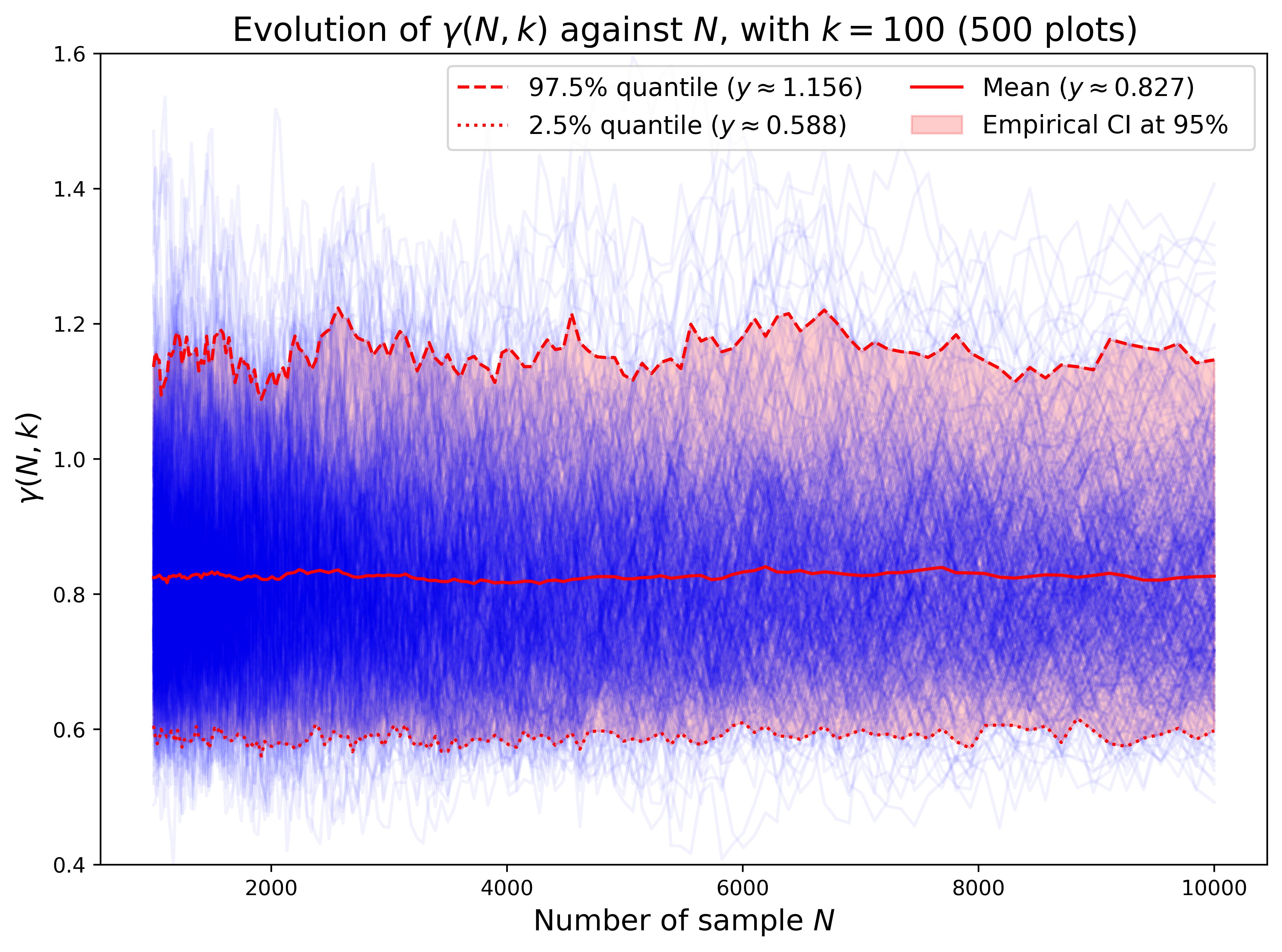
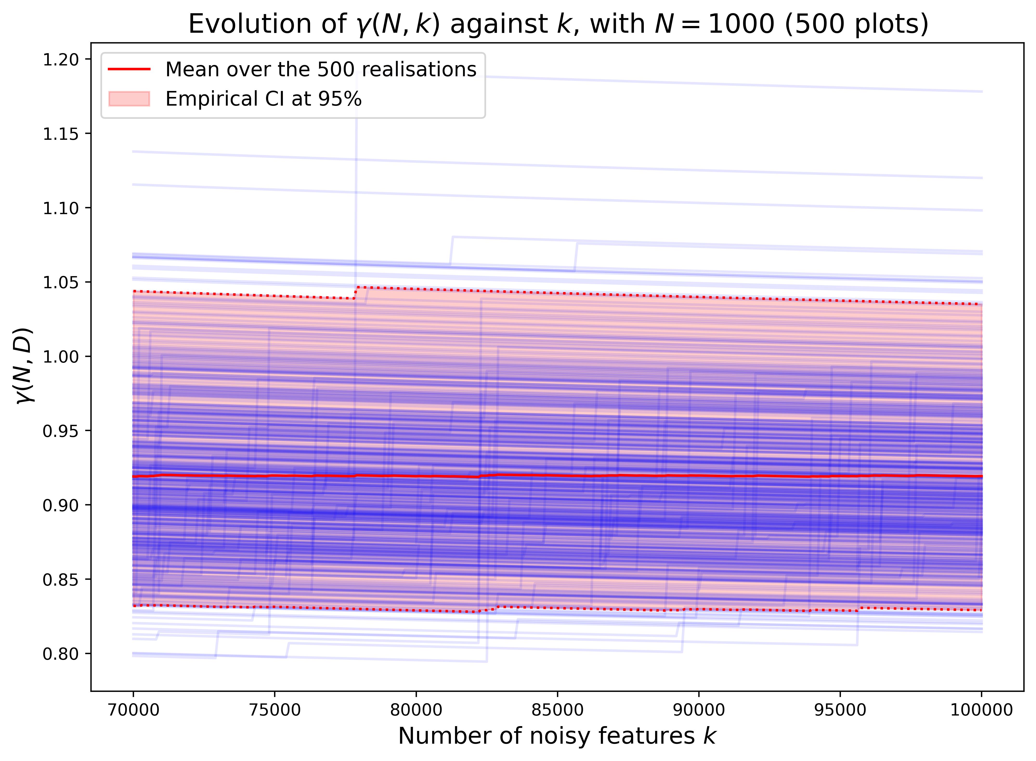
In order to verify empirically such a Conjecture, we start by dealing with tightness of $\gamma$ by generating a huge number of realisations of $\widehat{\xi}_{\mathrm{max}}$, which can be observed on Figures 2 and 3.

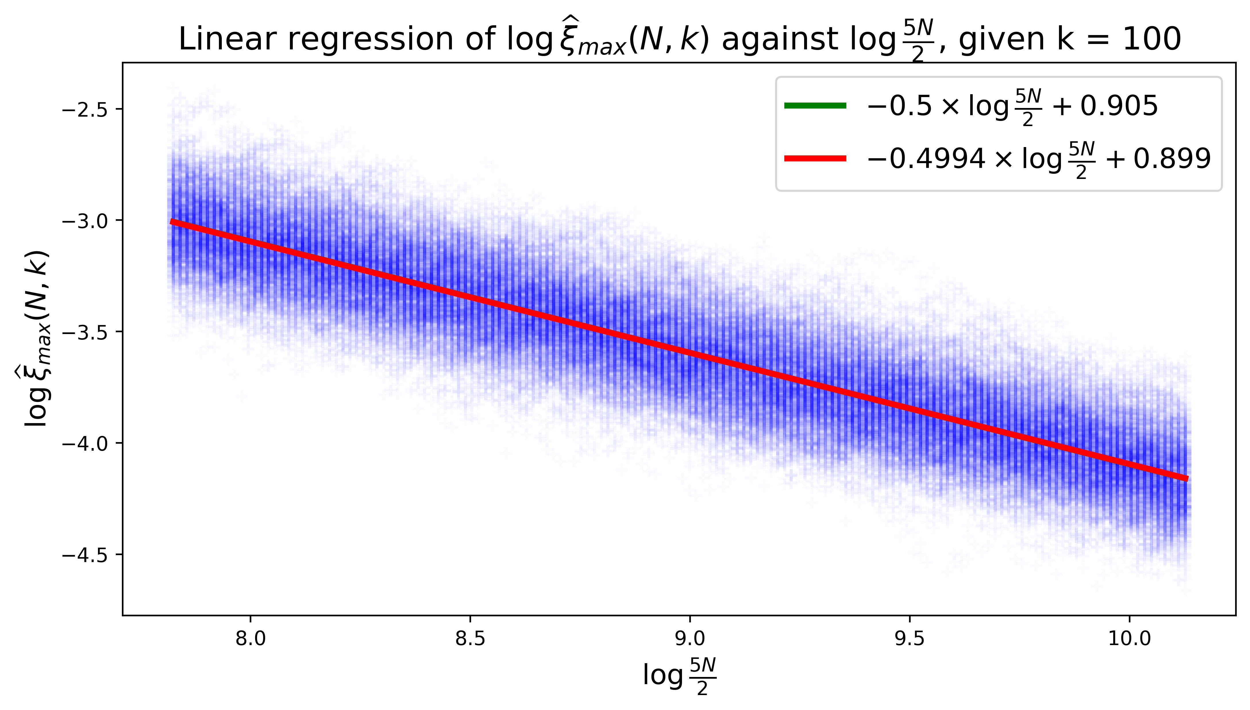
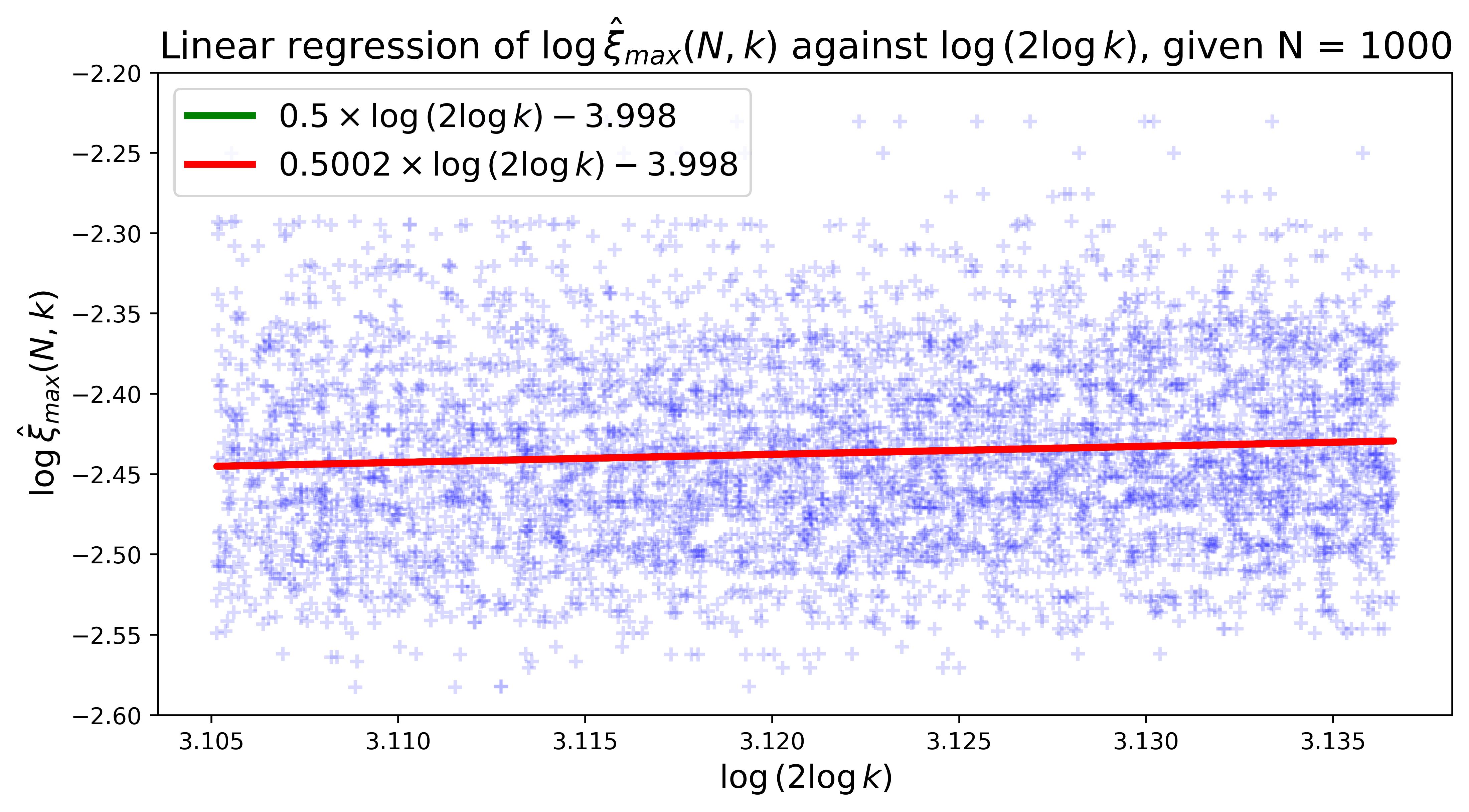
We also make some additional numerical experiments to test the relevance of Equation (8). Indeed, taking the logarithm, we obtain

$$\log\widehat{\xi}_{\mathrm{max}}(N,(i_{1},\dots,i_{k}))$$ (9)

$$= -\alpha_{1}\log\frac{5N}{2}+\beta_{1}\log\left(2\log(k)\right)+\log\gamma(N,k)\ ,$$

where

$$\alpha_{1}=\beta_{1}=\frac{1}{2}\ .$$

As $\log\gamma(N,k)$ is bounded with high probability, it can be treated as a residue. And the values of $\alpha_{1}$ and $\beta_{1}$ can be tested thanks to a classical Ordinary Least Squares (OLS) regression. The results in Figures 4 and 5 tend to confirm the conjecture as well.

Figure 2: Given $N_{\mathrm{max}}=10000$, $k=100$ and $P=500$, we generate $N_{\mathrm{max}}\times P$ i.i.d. realisations of mutually independent random variables $\left(X^{(1)},\dots,X^{(k)},Y\right)$, so that we have $P$ batches of $N_{\mathrm{max}}$ samples. On each of these batches, we use the $N_{\mathrm{max}}$ samples to compute $\widehat{\xi}_{\mathrm{max}}(N,(1,\dots,k))$ for $N\leq N_{\mathrm{max}}$. Thus, we obtain $P$ independent realisations of $\gamma(N,k)$ depending on $N<N_{\mathrm{max}}$, what we plot in blue.

Figure 3: Given $N=10\ 000$, $k_{\mathrm{max}}$ and $P=500$, we generate $N\times P$ i.i.d. realisations of mutually independent random variables $\left(X^{(1)},\dots,X^{(k_{\mathrm{max}})},Y\right)$, so that we have $P$ batches of $N$ samples. On each of these batches, we use the $N$ samples to compute $\widehat{\xi}_{\mathrm{max}}(N,(1,\dots,k))$ for $k\leq k_{\mathrm{max}}$. Thus, we obtain $P$ independent realisations of $\gamma(N,k)$ depending on $k<k_{\mathrm{max}}$, what we plot in blue.

Figure 4: We perform an (OLS) linear regression to estimate the slope $-\alpha_{1}$ in Equation (9). We obtain a confidence interval for $\alpha_{1}$ of $[0.498\ ,\ 0.501]$ with risk level at $95\%$.

Figure 5: We perform an (OLS) linear regression to estimate the slope $\beta_{1}$ in Equation (9). We obtain a confidence interval of $[0.497\ ;\ 0.504]$ with risk level at $95\%$.

IV Experiments

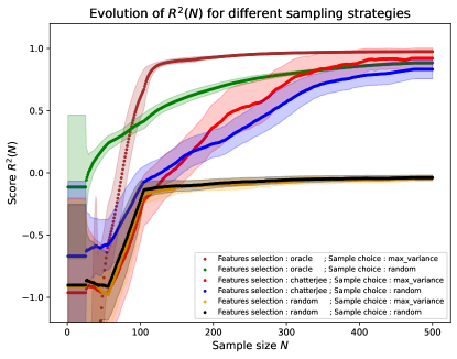
Variations of the flow: In order to assess the quality of our active sampling flow as described in Fig. 1, we consider different variations, in the feature selection and the sample choice. The different methods are listed in Table II and are motivated as follows.

	Feature selection	Choice of next sample
Method 1	GSA (Algorithm 2)	Maximal variance (Algorithm 1)
Method 2	GSA (Algorithm 2)	Random Choice
Method 3	Oracle Selection	Maximal variance (Algorithm 1)
Method 4	Oracle Selection	Random Choice
Method 5	Random Selection	Maximal variance (Algorithm 1)
Method 6	Random Selection	Random Choice

TABLE II: Variations of the active sampling flow of Fig. 1 during our experiments.

In the spirit of ablation studies, the choice of next sample can be done using the maximal variance criterion (Algorithm 1) or using a random choice. Regarding the feature selection, more variations are possible. A priori, the worst choice is a random selection. Then there is our feature selection based on sensitivity analysis (Algorithm 2). And finally there is the ideal case where we know of most relevant features thanks to an oracle.

For synthetic dataset obtained from the Sobol’ G-function, the oracle is simply the knowledge of the truly relevant variables during the dataset’s generation. For the HSOTA and the FIRC, the oracle is given by a sensitivity analysis performed on the entire dataset before launching the exploration.

Design of experiment and performance metric: We first start by separating our datasets into a training subset and a testing subset, according to a 75%-25% split ratio. Then, we perform the same following procedure for each method in Table II.

For any $N_{0}\leq N\leq N_{f}$, the (variant of the) active sampling flow provides a sample set

$${\mathcal{S}}_{N}=\left\{\left(x_{j},y_{j}\right)\in B\times{\mathbb{R}},\ 1\leq j\leq N\right\}\ ,$$

which is a subset of the training dataset. The sample ${\mathcal{S}}_{N}$ is used to train a Gaussian Process Regressor $\widehat{{\mathcal{F}}}_{N}$ over the selected features.

We are thus in position of computing an $R^{2}$ score on the testing dataset $\left(x^{test}_{j},y^{test}_{j}\right)_{1\leq j\leq N_{T}}$. For convenience, we recall the definition of the $R^{2}$ coefficient, also known as determination score

$$R^{2}(N)=1-\frac{\sum_{j=1}^{N_{T}}\left(y^{\mathrm{test}}_{j}-{\mathbb{E}}\left[{\mathcal{F}}_{N}\left(x^{\mathrm{test}}_{j}\right)\right]\right)^{2}}{\sum_{j=1}^{N_{T}}\left(y^{\mathrm{test}}_{j}-\overline{y}\right)^{2}}\ ,$$

where $\overline{y}$ is the mean

$$\overline{y}=\frac{1}{N_{T}}\sum_{j=1}^{N_{T}}y^{\mathrm{test}}_{j}\ .$$

In Figure 6, we illustrate the result graphically in the case of $F=G_{\mathrm{Sobol^{\prime}}}^{(d=4)}$. A more comprehensive account of the results will be given in a table.

Discussion: It seems that our flow (Method 1 - The original flow of Fig. 1) outperforms all other sampling methods, except for the Method 3, which is best case scenario using oracle a priori information.

Figure 6: We compute the mean $R^{2}(N)$ over $20$ runs for each method, as $N$ grows, as described through Section IV, for the dataset built from $G_{\mathrm{Sobol^{\prime}}}^{d=4}$.

V Conclusion

In this paper, we have shown the relevance of the statistical tools from sensitivity analysis, in order to design an active sampling flow for the characterization of analog circuits’ performances against a large number of variables representing sources of parametric variation. This active sampling flow outperforms Monte-Carlo sampling and we have illustrated the role of the different ingredients.

The framework is flexible enough to include surrogate models other than GPs, or to seek sampling criteria other than maximum variance. As such, one could include expert knowledge in the surrogate models or one could optimize for other criteria such as failure rates. This could be the topic of future research.

References

- [1] B. Bailey, “Adding circuit aging to variability.” https://semiengineering.com/adding-aging-to-variability, 2021.
- [2] S. Jallepalli, R. Mooraka, S. Parihar, E. Hunter, and E. Maalouf, “Employing scaled sigma sampling for efficient estimation of rare event probabilities in the absence of input domain mapping,” IEEE Transactions on Computer-Aided Design of Integrated Circuits and Systems, vol. 35, no. 6, pp. 943–956, 2016.
- [3] X. Shi, F. Liu, J. Yang, and L. He, “A fast and robust failure analysis of memory circuits using adaptive importance sampling method,” in Proceedings of the 55th Annual Design Automation Conference, pp. 1–6, 2018.
- [4] S. Yin, G. Dai, and W. W. Xing, “High-dimensional yield estimation using shrinkage deep features and maximization of integral entropy reduction,” in Proceedings of the 28th Asia and South Pacific Design Automation Conference, pp. 283–289, 2023.
- [5] Y. Liu, G. Dai, and W. W. Xing, “Seeking the yield barrier: High-dimensional sram evaluation through optimal manifold,” in 2023 60th ACM/IEEE Design Automation Conference (DAC), pp. 1–6, IEEE, 2023.
- [6] J. Zhai, C. Yan, S.-G. Wang, and D. Zhou, “An efficient bayesian yield estimation method for high dimensional and high sigma sram circuits,” in Proceedings of the 55th Annual Design Automation Conference, pp. 1–6, 2018.
- [7] S. Yin, X. Jin, L. Shi, K. Wang, and W. W. Xing, “Efficient bayesian yield analysis and optimization with active learning,” in Proceedings of the 59th ACM/IEEE Design Automation Conference, pp. 1195–1200, 2022.
- [8] C. K. Williams and C. E. Rasmussen, Gaussian processes for machine learning, vol. 2. MIT press Cambridge, MA, 2006.
- [9] I. Azzini and R. Rosati, “A function dataset for benchmarking in sensitivity analysis,” Data in Brief, vol. 42, p. 108071, 2022.
- [10] Wikipedia contributors, “Operational transconductance amplifier — Wikipedia, the free encyclopedia.” https://en.wikipedia.org/w/index.php?title=Operational_transconductance_amplifier&oldid=1214653053, 2024. [Online; accessed 23-April-2024].
- [11] Wikipedia contributors, “Clock signal — Wikipedia, the free encyclopedia.” https://en.wikipedia.org/w/index.php?title=Clock_signal&oldid=1217842343, 2024. [Online; accessed 23-April-2024].
- [12] Cadence, “Circuit simulation.” https://www.cadence.com/en_US/home/tools/custom-ic-analog-rf-design/circuit-simulation.html, 2024. [Online; accessed 23-April-2024].
- [13] F. Gamboa, T. Klein, A. Lagnoux, and L. Moreno, “Sensitivity analysis in general metric spaces,” Reliability Engineering & System Safety, vol. 212, p. 107611, 2021.
- [14] S. Chatterjee, “A new coefficient of correlation,” Journal of the American Statistical Association, vol. 116, no. 536, pp. 2009–2022, 2021.
- [15] M. R. Leadbetter, G. Lindgren, and H. Rootzén, Extremes and related properties of random sequences and processes. Springer Science & Business Media, 2012.