Scene Action Maps: Behavioural Maps for
Navigation without Metric Information

Abstract

Humans are remarkable in their ability to navigate without metric information. We can read abstract 2D maps, such as floor-plans or hand-drawn sketches, and use them to navigate in unseen rich 3D environments, without requiring prior traversals to map out these scenes in detail. We posit that this is enabled by the ability to represent the environment abstractly as interconnected navigational behaviours, e.g., “follow the corridor” or “turn right”, while avoiding detailed, accurate spatial information at the metric level. We introduce the Scene Action Map (SAM), a behavioural topological graph, and propose a learnable map-reading method, which parses a variety of 2D maps into SAMs. Map-reading extracts salient information about navigational behaviours from the overlooked wealth of pre-existing, abstract and inaccurate maps, ranging from floor-plans to sketches. We evaluate the performance of SAMs for navigation, by building and deploying a behavioural navigation stack on a quadrupedal robot. Videos and more information is available at: https://scene-action-maps.github.io.

I Introduction

Can robots navigate with limited metric and spatial information, just as humans do? Currently, most robots’ navigation systems rely on detailed geometric maps and accurate metric positioning [1]. Yet humans can often find their way to their destinations guided only by abstract, inaccurate representations of the environment - e.g., hand-drawn sketches or language-based directions - and approximate, semantic notions of their position. A key enabler of this skill is our ability to represent and navigate environments using navigational behaviours, which are semantic action abstractions like turn left or follow corridor. Humans can use geometrically inaccurate maps or representations because these still capture paths in the environment abstractly, as sequences of navigational behaviours: e.g. floor-plans allow us to infer the abstract sequences of turning and corridor following actions to take to reach a given room, despite their lack of realism. We can also perceive navigational affordances [2], i.e. the potential in the local environment for executing a navigational behaviour, and use them as non-metric, visual cues of our location: e.g. observing that a nearby junction only affords us the chance to turn left and go forward can hint at our location in a building. We hypothesise that using navigational behaviours to represent and traverse environments imbues robots with the ability to navigate with limited metric and spatial information.

To test this hypothesis, we design a navigational behaviour-based robot system centred on the Scene Action Map (SAM), a topological representation comprising key places (nodes) joined by navigational behaviours (edges), that supports non-metric planning and localisation. In particular, we propose a learnable map-reading pipeline to extract SAMs from various kinds of readily available, pre-existing 2D maps of the environment - e.g. hand-drawn sketches and floor-plans. While many systems struggle to use such maps due to their metric inaccuracies and abstractness, ours instead uses the underlying SAMs encoded in these maps, allowing us to exploit this wealth of pre-existing map information.

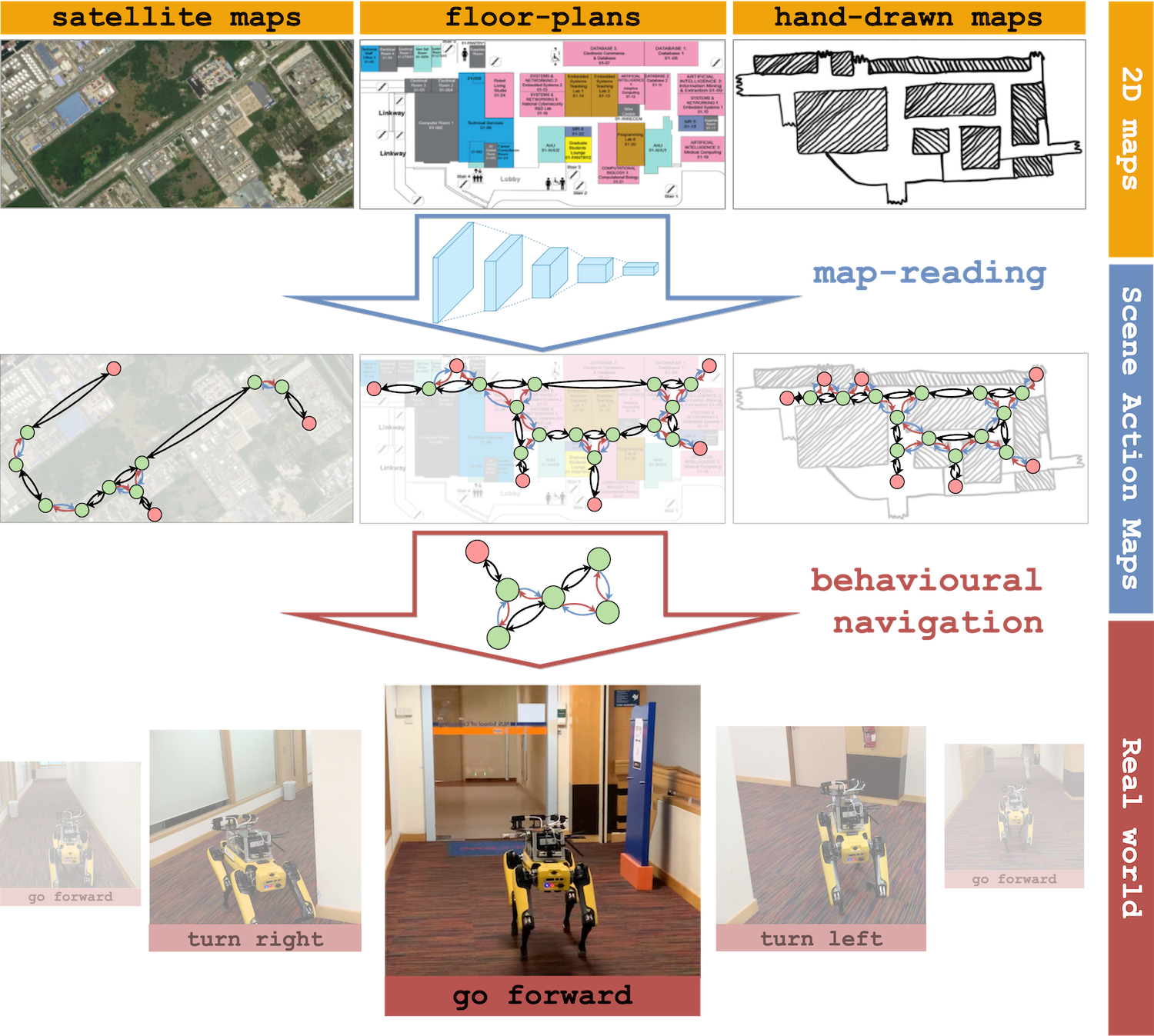
Figure 1: We propose a learnable map-reading system that extracts Scene Action Maps from pre-existing 2D maps, for behavioural navigation.

Prior work in visual navigation has shown the practicality of learning human-like navigational behaviours [3, 4, 5] and localising with their associated navigational affordances [6]. Building on these, we implement a behavioural navigation stack employing SAMs and deploy it on a real robot to validate the usefulness of the extracted SAMs for navigation. In particular, we use the DECISION controller’s obstacle-avoiding navigational behaviours [5] and adapt Graph Localisation Networks [6] for affordance-based localisation. We “read” SAMs from hand-drawn maps, floor-plans and satellite maps, and demonstrate that these extracted SAMs can be used for effective real-world navigation.

II Related Work

Many robot navigation systems rely on accurate metric positioning and detailed geometric maps built with sensor data collected first-hand from the target environment [1]. However, metric accuracy remains challenging to achieve in general: existing SLAM methods are sensitive to sensing conditions and robot dynamics, and can be difficult to extend to large-scale environments [7]. Further, by focusing on map-building with first-hand sensor data, these systems ignore the rich source of prior information for navigation provided by the wealth of pre-existing maps of manmade environments.

II-A Navigation without metric information

To tackle the problems that metric inaccuracies pose for navigation, some works aim to improve the quality of metric mapping and localisation under challenging conditions [8, 9, 10]. In contrast, our work follows the approach of reducing the dependence of navigation on metric information.

A common strategy is to design navigation systems that only assume local metric consistency. Such systems typically navigate with topometric maps comprising independent metric submaps each with their own local reference frame, connected by a global graph [11, 12, 13, 14, 15]. Localisation and motion planning are done with respect to the submap the robot is currently in. While this helps to deal with issues like map corruptions owing to drift over long distances, it still depends on high metric accuracy locally within the submaps.

Purely topological approaches go further by avoiding metric information, instead representing the world relationally as a graph of perceptually significant places [16]. A key challenge lies in grounding abstract topological routes to real-world metric paths and actions. Various action primitives, or behaviours, are used to bridge symbolic topological maps and the real world: Spatial Semantic Hierarchy and similar works use wall-following behaviours to travel between nodes [17, 18, 19], while [20] uses a visual servoing behaviour that takes image goals. However, these are often simple, handcrafted policies that can be brittle in the real world.

Deep learning provides a means of implementing robust behaviours, shown by its success in learning reactive visuomotor policies [4, 21, 22, 23, 24, 5]. Recent works use this to imbue purely topological approaches with robust locomotion. SPTM [25] and RECON [26] build reachability graphs of the environment and learn image goal conditioned visuomotor policies to navigate between nodes. While these policies only consider the basic navigational affordance of reachability, [3, 6] learn behaviour sets for indoor environments that exploit more semantically meaningful affordances: e.g., entering/exiting afforded by doors, path-following afforded by corridors etc. These affordances are associated with strong visual cues that help to guide behaviour execution, and are used in [6] to localise on a topological map.

Our SAM-based system is a topological, behavioural navigation system that builds on [6]. While [3, 6] assume the graph is given, we propose to build SAMs from pre-existing maps. We also use the driving direction-based behaviours of [24, 5], which apply to a wider range of environments. Lastly, while many prior works only evaluate their systems in simulation, we test ours in the real world.

II-B Navigation with pre-existing environment information

While most SLAM approaches can only build maps for navigation from first-hand sensor data, some works build alternative navigation systems that leverage readily available, pre-existing maps for guidance, like hand-drawn sketches [27, 28] or architectural floor-plans [29, 30]. These are tailored to specific map types and make strong assumptions: the former assumes the sketch is a diffeomorphism of 2D LiDAR data, while the latter assumes mostly metrically accurate floor-plans. The I-Net system [24] lowers accuracy needed in the latter by translating planned paths into sequences of path-following navigational behaviours, each locally guided by visual cues and affordances. However, it relies on metric localisation to switch between behaviours, and can fail under severe inaccuracies. Instead of tailoring navigation to specific map types, other works extract general intermediate representations for navigation: e.g. road networks from aerial images/satellite maps [31, 32, 33].

This work proposes SAMs as a fully topological, general intermediate representation that can be extracted from a wide variety of readily available, pre-existing map types, ranging from sketches to floor-plans to satellite maps. Unlike prior approaches handcrafted for specific map types, our learnable “map-reading” system can be trained to extract SAMs from different map types for navigation.

III Methodology

We consider the task of navigating to goals in environments the robot may not have seen or explored before. This naturally requires navigation with limited metric and spatial information, as lack of prior data means detailed geometric maps for planning and localisation may be unavailable. However, we assume access to readily available, pre-existing 2D maps of the environment like floor-plans, hand-drawn maps and satellite maps. Though they may be abstract and inaccurate, they retain information about the environment’s navigational affordances useful for planning and localisation.

Some key challenges of this task include specifying goals, planning and localising with a range of abstract, inaccurate maps. Our approach is to extract a behavioural, topological graph of the environment from the maps, i.e. a Scene Action Map (SAM), and navigate with it. We assume access to a set of navigational behaviours like DECISION [5], that are capable of local obstacle avoidance and diverse enough to allow us to reach most places in the target environment. Our offline map-reading system is a learnable pipeline that, given a specific behaviour set, can be trained to extract SAMs from a variety of 2D maps. The online behavioural navigation system takes in a goal specified on the SAM, plans a path over the SAM and executes it. Since we cannot depend on having accurate metric information, we use affordance-based localisation and learned navigational behaviours.

III-A Scene Action Map

A SAM is a directed graph $\mathcal{G}=(\mathcal{V},\mathcal{E})$. Each node $v\in\mathcal{V}$ stores a single label, marking it as a changepoint or destination node. Changepoint nodes denote locations at which the robot is afforded the chance to transition between behaviours. For example, a changepoint may be placed just before a cross-junction, since the junction affords the robot the chance to switch from going forward to turning left. These nodes are extracted from pre-existing maps via offline map-reading. As the user may also want to set goals at places that are not changepoints, we allow them to specify destination nodes. The map-reading system takes in such nodes and includes them when forming the SAM.

Each directed edge $e\in\mathcal{E}$ stores a single label specifying the required navigational behaviour to move between its start and end nodes. The behaviours are drawn from a predefined set of $N$ navigational behaviours. In principle, SAMs can be adapted to use different behaviour sets.

We enforce the structural constraint that for any node $v$, each outgoing edge has a unique behaviour, implying $v$ has $\leq N$ outgoing edges. Intuitively this avoids the ambiguity of $v$ having multiple outgoing edges of the same behaviour type leading to different destinations, ensuring the problem of localising on a SAM is well-defined.

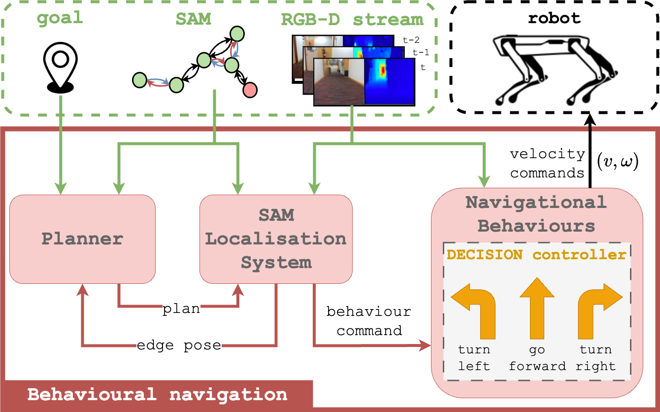
Figure 2: Overview of the online behavioural navigation system.

III-B Online navigation with SAMs

To navigate to a specified goal, the online behavioural navigation system (Figure 2) finds a valid path over the SAM with the planner, then executes it with learned navigational behaviours. The robot’s position on the SAM is estimated by the SAM localisation system (SLS).

Navigational behaviours: These are a set of traversability-aware learned visual navigation policies that exploit navigational affordances. We use the DECISION controller [5] which learns {turn-left, go-forward, turn-right} path-following behaviours with obstacle avoidance. These are meant to navigate along clearly defined paths, and may not handle areas like open spaces well. Regardless, our approach is not specific to this behaviour set, and can potentially be extended to other behaviours.

SAM localisation system (SLS): Like Graphnav [6], our system estimates the robot’s pose as the edge of the SAM it is currently on. This edge pose is better defined than specifying the robot’s pose as a node, since the robot may not always be near a node but is always executing an edge.

The SLS processes a sequence of depth images and a “crop” (local neighbourhood) of the SAM around the last edge pose. It estimates the current edge pose and triggers a behaviour switch command when nearing a changepoint. The SLS comprises a Graph Localisation Network (GLN) modified from Graphnav, a changepoint detector and edge pose predictor. The GLN encodes the image sequence into a feature vector capturing the local environment’s structure and navigational affordances. It uses a GNN to match this vector with features encoding the SAM’s topology and behaviour information, assigning scores to edges based on their likelihood to be the edge pose. The edge pose predictor temporally smooths these “edge scores” and returns the best-scoring edge as the edge pose. Unlike Graphnav, we add a 3-layer MLP head to our GLN’s last graph network block, that maps a given edge’s features to a score indicating proximity to the changepoint at the edge’s end. The changepoint detector temporally smooths and thresholds this “changepoint score” to determine changepoint proximity, and prompts a transition to the next planned behaviour if nearby.

We found explicit changepoint detection crucial for the robot to anticipate upcoming behaviour transitions. Slight lag in edge pose predictions from filtering, combined with our robot’s higher speeds ($\sim$0.8m/s) compared to Graphnav’s ($\sim$0.5m/s) meant our robot could overshoot the changepoint before a behaviour switch could occur. Predicting changepoint proximity provides a mechanism to anticipate this switch and change behaviours in time.

Let p be a vector of unnormalized edge scores from the SAM crop, and $\textbf{q}_{gt}$ a vector of the ground truth edge pose’s unnormalized changepoint scores. We train the GLN with cross-entropy losses on both p and $\textbf{q}_{gt}$:

$$\mathcal{L}_{GLN}(\textbf{p},\textbf{q}_{gt})=\mathcal{L}_{xent}(\textbf{p})+\lambda\mathcal{L}_{xent}(\textbf{q}_{gt}).$$ (1)

Planner: Given a goal node, the planner searches over the SAM for a path from the current edge pose using Dijkstra. If a path exists, the planner returns a sequence of edges, and hence a sequence of behaviours to execute. During execution, the planner replans if the robot’s edge pose deviates from the path. Since behaviours represent semantically meaningful, human-like actions, each plan is inherently interpretable.

We note that our changepoint detector lets us halt near goal nodes that are changepoints. For destination nodes, we heuristically halt after moving a preset distance along the edge leading to it. We do this since destinations are often near changepoints in indoor areas: e.g., reaching a room usually involves stopping shortly after entering and crossing the entrance changepoint. An alternative approach could have users label destination nodes with semantic location information (e.g., “near desk in office”) to guide the robot on when/where to halt.

III-C Offline map-reading

The diverse appearance of common, pre-existing 2D maps makes it challenging to handcraft general algorithms to extract SAMs from all map types. Instead, we propose a general pipeline that can be trained to extract SAMs from specific map types, given data of that map type. SAM prediction can be sequentially decomposed into node prediction, followed by edge prediction to connect the nodes with appropriate behaviours. We learn neural networks $\phi_{node}$ and $\phi_{edge}$ to aid in node and edge prediction. For a given map type and set of behaviours, if we can curate a dataset of such maps annotated with SAMs, we can train instances of $\phi_{node}$ and $\phi_{edge}$ to predict SAMs for that map type.

Node prediction: This takes in a 2D map $\mathcal{M}$ and yields $\mathcal{V}$, the set of nodes in the SAM. We learn $\phi_{node}$, a CNN that takes a patch from the map centred on a point, and outputs the likelihood that the point is a changepoint. Algorithm 1 details how $\phi_{node}$ is used to score points sampled from the map and cluster them to extract the set of changepoints in the map, $\mathcal{P}_{c}$. We return the set of nodes in the SAM $\mathcal{V}=\mathcal{P}_{c}\cup\mathcal{P}_{d}$, where $\mathcal{P}_{d}$ is the set of user-specified destination nodes. $\phi_{node}$ is trained in two stages: we first learn a latent representation of changepoints using supervised contrastive learning (SupCon) [34], then add an MLP head and finetune the network to classify changepoints with a binary cross-entropy loss. Training data consists of positive samples drawn from a small neighbourhood around annotated changepoints, and negative samples from the rest of the map. We use SupCon as it allows us to exploit our data’s positive/negative labels and learn a class-based representation. We find such contrastive representation learning to be essential for good convergence and achieving good changepoint predictions.

Algorithm 1 Changepoint node prediction

0:  2D map $\mathcal{M}$, grid res $r$, changepoint threshold $\beta_{cp}$

0:  Set of changepoints: $\mathcal{P}_{c}$

1:  $\mathcal{P}\leftarrow$ Grid-sampled points from $\mathcal{M}$ with resolution $r$

2:  $\mathcal{P}_{filtered}\leftarrow\{\}$;

3:  for each $p\in\mathcal{P}$ do

4:     $m_{p}\leftarrow$ Crop image patch centred on $p$ from $\mathcal{M}$;

5:     $s_{p}\leftarrow$ $\phi_{node}$($m_{p}$), i.e. likelihood $p$ is a changepoint;

6:     if $s_{p}>\beta_{cp}$ then

7:        $\mathcal{P}_{filtered}\leftarrow\mathcal{P}_{filtered}\cup\{p\}$;

8:  Extract set of approximately convex clusters $\mathcal{C}$ from $\mathcal{P}_{filtered}$ with GrowCompactClusters from [35];

9:  $\mathcal{P}_{c}\leftarrow$ Set of points with highest $s_{p}$ from each $c\in\mathcal{C}$;

10:  return  $\mathcal{P}_{c}$

Edge prediction: This takes in a 2D map $\mathcal{M}$ and the set of nodes $\mathcal{V}$, and returns $\mathcal{E}$, the set of edges in the SAM. We compute $\mathcal{E}=\bigcup\limits_{v_{i}\in\mathcal{V}}E_{v_{i}}=\bigcup\limits_{v_{i}\in\mathcal{V}}f_{ep}{}(v_{i},\mathcal{M})$, where $f_{ep}{}$ predicts the set of outgoing edges from $v_{i}\in\mathcal{V}$ while satisfying the SAM structural constraints. Intuitively, $f_{ep}{}$ finds a partial assignment between behaviours and possible outgoing edges from $v_{i}$ under these constraints. Since $f_{ep}{}$ must be learnable to adapt to different map types, we solve this optimisation differentiably with the Sinkhorn algorithm [36]. This lets us predict the input score matrix to the Sinkhorn layer with a neural network, and learn to use visual information from $\mathcal{M}$ for edge prediction. For $N$ behaviours and $K$ nearest neighbour nodes to $v_{i}$, the score matrix has size $K\times N$. Intuitively the $(k,n)$-th element scores how likely it is that the SAM contains edge $e_{ik}$ with behaviour $n$. Like [37], we pad our score matrix with a “dustbin” row and column to allow for partial assignments. The Sinkhorn layer yields a soft assignment matrix $X$, that is thresholded during inference to get $E_{v_{i}}$.

Concretely, $f_{ep}{}$ comprises $\phi_{edge}$ (Figure 3) followed by a Sinkhorn layer. $\phi_{edge}$ is af CNN that predicts the score matrix from a $(3+K)$-channel input, where the first 3 channels are a crop of $\mathcal{M}$ around $v_{i}$, and the $(3+k)$th channel is a binary image with the $k$th neighbouring node’s location rasterised on it. In practice $\phi_{edge}$’s fixed-size receptive field cannot easily handle environments where nodes can be very far apart, e.g. at the ends of a long corridor. We tackle this with a multi-scale approach that learns separate $\phi_{edge}$ networks to run $f_{ep}{}$ at several scales. The edge predictions across scales are heuristically merged by preferring shorter pixel space edges. We learn a representation for $\phi_{edge}$ with SupCon before finetuning it to predict edges. Given ground truth assignment matrix $A$, the loss for finetuning is:

$$\mathcal{L}_{assign}=-\frac{1}{\lVert A\rVert^{2}_{F}}\sum\limits_{n=1}^{N}\sum\limits_{k=1}^{K}a_{nk}\log(x_{nk}).$$ (2)

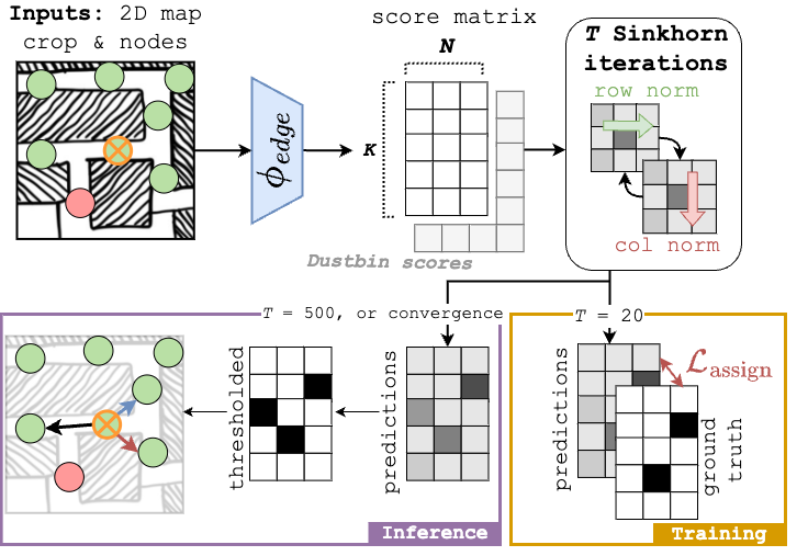
Figure 3: Applying $f_{ep}{}$ to orange marked node: 1) predicts soft assignment matrix with $\phi_{edge}$ and Sinkhorn, 2) thresholds to yield the outgoing edges.

III-D Implementation details

$\phi_{node}$ is a MobileNetv2 with 4-layer MLP, trained with batch size 64, learning rates of $10^{-2}$ for SupCon and $10^{-4}$ for finetuning. $\phi_{edge}$ is a MobileNetv2 with 3-layer MLP whose output is reshaped into the score matrix. We use learning rates/batch sizes of $10^{-2}/64$ for SupCon and $10^{-3}/32$ for finetuning. We train GLNs following Graphnav’s method [6], and add data augmentation during training by randomly changing the assigned behaviour of a single edge in the SAM crop.

IV Experiments

Our experiments aim to answer the questions:

1. How well can our offline map-reading approach extract SAMs from varied 2D map inputs?

2. Is our online behavioural navigation system practical for real-world navigation? Do our proposed modifications to the GLN improve real-world performance?

3. How well can the robot navigate using SAMs extracted by the offline map-reading system?

IV-A Map-reading

TABLE I: Precision and Recall over various 2D map types for (A) node prediction, (B) edge prediction alone (ignoring behaviour correctness), (C) edge and behaviour prediction

	Hand		Flr		SatMap
Tasks	Pr	Re	Pr	Re	Pr	Re
(A)	0.848	0.975	0.732	0.779	0.865	0.621
(B)	0.754	0.605	0.820	0.643	0.863	0.751
(C)	0.667	0.535	0.630	0.494	0.761	0.662

We collect data for the 3 map types in Figure 1: hand-drawn maps (Hand) and floor-plans (Flr) of campus buildings, and satellite maps (SatMap) of industrial areas. SAMs are manually annotated for maps in Hand and Flr datasets. SAMs are annotated using OpenStreetMap road/junction information for SatMap maps. We train a separate instance of our map-reading module for each map type. To answer Q1, we test on held-out datasets: Hand/Flr each have 4 maps with each map having a mean of 27 nodes and 64 edges, and SatMap has 1 large map with 137 nodes and 414 edges. We compute precision and recall for 3 tasks: (A) predicting nodes/changepoints, (B) predicting edges alone (disregarding behaviour correctness), and (C) predicting edges along with their associated behaviours. Intuitively (B) shows how well the environment’s structure and connectivity is captured. (C) further checks each edge’s assigned behaviour against human-annotated maps. Results are presented in Table I.

Our node prediction performs well at predicting changepoints across all map types. Qualitatively, $\phi_{node}$ is able to reliably capture visual features in the maps, like junctions or turnings, that can indicate a changepoint when using the DECISION behaviour set. Failures mainly occur in open areas where the environment’s structure is less well-defined, leading to more false positives and negatives. The comparatively lower recall score for SatMap is mostly due to features like junctions being occluded by tall buildings in densely built-up areas, inducing more false negatives.

Our edge prediction performs well on task (B), particularly on SatMap due to the rich visual information inherent in satellite maps. The lower recall scores indicate that $f_{ep}{}$’s main limitation is its occasional failure to identify valid edges. Lower performance on task (C) compared to (B) suggests that while $\phi_{edge}$ can learn reachability between nodes well, it is significantly more challenging to learn the right visual features needed to assign correct behaviours. This is supported by the observation that most failures involve a go-forward behaviour being wrongly assigned as a turning behaviour and vice versa.

We connect node and edge prediction, and generate SAMs end-to-end in Figure 4. Our method can trace out connected graphs that capture the topology of the map reasonably accurately. While there is some noise in the predicted SAMs - in the form of missing changepoints, edges with mislabelled behaviours etc. - we demonstrate that these SAMs can still be effectively used for behavioural navigation.

IV-B Indoor robot navigation

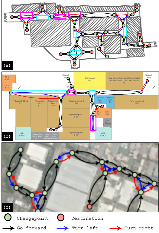
Figure 4: SAMs extracted from (a) hand-drawn maps, (b) floor-plans, (c) satellite maps. The SAMs mostly capture the behaviours and environment structure accurately, apart from occasional errors (circled on maps) like confusing go-forward and turning edges, or missing edges.

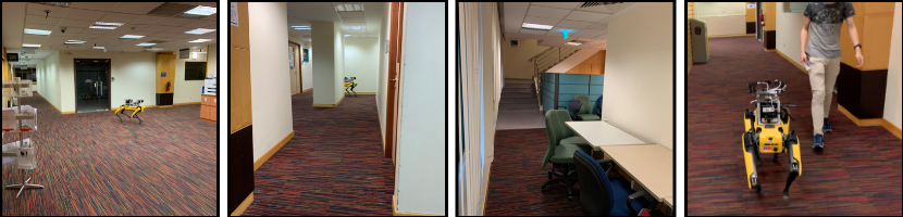
Figure 5: Navigating our test environment is a challenge due to (left-to-right) wide open spaces, complex junctions, cluttered areas and dynamic obstacles.

We run the online behavioural navigation system on a Boston Dynamics Spot robot with an AGX Xavier and 3 Realsense d435i RGB-D cameras with combined 140^∘ FoV.

Our navigation tests are split into 3 difficulty levels based on the number of changepoints the robot must transit through: Easy (2-3 changepoints over 10-25m), Medium (4-5 changepoints over 30-50m), and Hard (6-10 changepoints over 50-100m). All changepoints in the SAM are included in the Easy and Medium routes. Hard routes involve a circuit around the entire building level being tested. Graphnav [6] defines difficulty differently: their corresponding levels contain paths with 1-10 nodes, 11-20 nodes and 21-30 nodes. Their paths are shorter despite having more nodes (median/maximum lengths of 30/60m). Since nodes are closely packed in their environment, their robot easily accumulates ample topological features to localise. In contrast, our environments contain long corridors with sparse junctions and changepoints, forcing our GLN to localise with sparser features. Our real-world tests also include complex environment structure and distractors (Figure 5), making navigation harder than in Graphnav’s simulation tests.

Like Graphnav, we assess navigation performance using Success Rate (SR) and Plan Completion (PC). PC is the proportion of nodes on the path successfully transited through. Based on SR and PC, we define two finer-grained sets of metrics: SR-Nav and PC-Nav to capture overall system performance, and SR-HL and PC-HL to capture the performance of the high-level navigation system - i.e. planner and localisation - in isolation. For the Nav metrics, failure is if an incorrect behaviour is issued or a behaviour fails. For HL, failure only occurs if an incorrect behaviour is issued: a controller failure is manually corrected by the operator.

To answer Q2, we find that the behavioural navigation system using our proposed SAM Localisation System (SLS) performs well on all routes when given high-quality, human-annotated (HA) SAMs, specifically hand-drawn maps (Hand-HA) and floor-plans (Flr-HA). Our SLS outperforms Graphnav’s localisation system GLN-Heu, which combines their vanilla GLN with heuristics that use the edge probability distribution to decide when to switch behaviours. This is due to GLN-Heu’s failure to switch behaviours in time, which SLS mitigates with changepoint proximity detection.

We answer Q3 by showing that effective behavioural navigation is possible with “noisy” predicted SAMs, which may contain defects such as edges labelled with the wrong behaviours or missing nodes/edges (see Figure 4). We evaluate both SLS and SLS-Aug on noisy SAMs, with SLS-Aug using a GLN trained with our proposed data augmentations for enhanced noise robustness. We draw 2 conclusions from Table II. Firstly, navigation performance experiences minimal adverse effects when substituting noisy predicted SAMs for human-annotated SAMs, indicated by the fact that SLS systems see at most a small drop in PC between human-annotated and predicted SAMs. Empirically, SLS and SLS-Aug seem robust to the common modes of noise - i.e. missing edges at a junction or confusing go-forward and turning behaviours - and is often able to use the remaining correct topological features to localise and navigate. Secondly, our data augmentation improves localisation and navigation on predicted SAMs containing noise and artifacts. On predicted SAMs, SLS-Aug generally outperforms other test settings, and even surpasses SLS on human-annotated SAMs. Overall, SLS-Aug shows promising performance even on Hard routes of up to 100m with multiple changepoint transitions, affirming the feasibility of predicting SAMs from 2D maps to localise and navigate in the real world.

TABLE II: Comparing navigation performance on human-annotated (HA) SAMs with GLN-Heu (Graphnav) and our SLS, and on noisy, predicted SAMs with SLS and SLS-Aug

Test settings		SR-HL	PC-HL	SR-Nav	PC-Nav
Easy	Hand-HA (GLN-Heu)	45.5	56.8	45.5	52.3
	Hand-HA (SLS)	70.0	85.0	70.0	85.0
	Hand (SLS)	70.0	85.0	70.0	85.0
	Hand (SLS-Aug)	80.0	90.0	80.0	90.0
	Flr-HA (GLN-Heu)	12.5	43.8	12.5	43.8
	Flr-HA (SLS)	66.7	77.8	66.7	77.8
	Flr (SLS)	88.9	94.4	88.9	94.4
	Flr (SLS-Aug)	68.8	78.1	62.5	71.9
Med	Hand-HA (GLN-Heu)	12.5	21.9	12.5	21.9
	Hand-HA (SLS)	50.0	87.5	50.0	81.3
	Hand (SLS)	75.0	84.4	62.5	75.0
	Hand (SLS-Aug)	75.0	87.5	62.5	75.0
	Flr-HA (GLN-Heu)	0.0	18.8	0.0	12.5
	Flr-HA (SLS)	37.5	62.5	12.5	43.8
	Flr (SLS)	22.2	56.7	22.2	56.7
	Flr (SLS-Aug)	37.5	65.6	37.5	65.6
Hard	Hand-HA (GLN-Heu)	0	12.5	0	12.5
	Hand-HA (SLS)	50.0	75.0	50.0	75.0
	Hand (SLS)	0	71.7	0	71.7
	Hand (SLS-Aug)	50.0	85.0	50.0	85.0
	Flr-HA (GLN-Heu)	0	15.8	0	15.8
	Flr-HA (SLS)	0	73.9	0	73.9
	Flr (SLS)	0	33.3	0	33.3
	Flr (SLS-Aug)	50.0	80.0	50.0	80.0

V Conclusion

We introduced Scene Action Maps, a behavioural topological representation for navigation. We recognise that common, pre-existing maps like floor-plans often encode information on navigational affordances and behaviours, and propose a “map-reading” system to extract SAMs from such maps. We also show effective real-world navigation with SAMs extracted from sketches and floor-plans.

SAMs make a trade-off: by being constrained to specific behaviour sets (and hence robot dynamics) they reduce reliance on metric information. In contrast, geometric maps need accurate data and cannot be built from abstract inputs, but represent the world richly enough to enable navigation with a wide range of robot dynamics. In future work, we intend to test our system in outdoor environments and incorporate richer sources of information into SAMs.

References

- [1] R. Siegwart, I. Nourbakhsh, and D. Scaramuzza, Introduction to autonomous mobile robots. MIT press, 2011.
- [2] M. Bonner and R. Epstein, “Coding of navigational affordances in the human visual system,” Proceedings of the National Academy of Sciences, vol. 114, p. 201618228, 04 2017.
- [3] G. Sepulveda, J. C. Niebles, and Á. Soto, “A deep learning based behavioral approach to indoor autonomous navigation,” 2018 IEEE International Conference on Robotics and Automation (ICRA), pp. 4646–4653, 2018.
- [4] M. Sorokin, J. Tan, C. K. Liu, and S. Ha, “Learning to navigate sidewalks in outdoor environments,” IEEE Robotics and Automation Letters, vol. 7, no. 2, pp. 3906–3913, 2022.
- [5] B. Ai, W. Gao, Vinay, and D. Hsu, “Deep visual navigation under partial observability,” in 2022 International Conference on Robotics and Automation (ICRA), 2022, pp. 9439–9446.
- [6] K. Chen, J. P. de Vicente, G. Sepulveda, F. Xia, A. Soto, M. Vázquez, and S. Savarese, “A behavioral approach to visual navigation with graph localization networks,” in Proceedings of Robotics: Science and Systems, FreiburgimBreisgau, Germany, June 2019.
- [7] C. Cadena, L. Carlone, H. Carrillo, Y. Latif, D. Scaramuzza, J. Neira, I. Reid, and J. Leonard, “Simultaneous localization and mapping: Present, future, and the robust-perception age,” IEEE Transactions on Robotics, vol. 32, 06 2016.
- [8] J. Zhang and S. Singh, “Visual-lidar odometry and mapping: low-drift, robust, and fast,” 2015 IEEE International Conference on Robotics and Automation (ICRA), pp. 2174–2181, 2015. [Online]. Available: https://api.semanticscholar.org/CorpusID:6054487
- [9] K. Ebadi, Y. Chang, M. Palieri, A. Stephens, A. Hatteland, E. Heiden, A. Thakur, N. Funabiki, B. Morrell, S. Wood, L. Carlone, and A.-a. Agha-mohammadi, “Lamp: Large-scale autonomous mapping and positioning for exploration of perceptually-degraded subterranean environments,” in 2020 IEEE International Conference on Robotics and Automation (ICRA), 2020, pp. 80–86.
- [10] Y. Chang, K. Ebadi, C. E. Denniston, M. F. Ginting, A. Rosinol, A. Reinke, M. Palieri, J. Shi, A. Chatterjee, B. Morrell, A.-a. Agha-mohammadi, and L. Carlone, “Lamp 2.0: A robust multi-robot slam system for operation in challenging large-scale underground environments,” IEEE Robotics and Automation Letters, vol. 7, no. 4, pp. 9175–9182, 2022.
- [11] M. Bosse, P. Newman, J. Leonard, and S. Teller, “Simultaneous localization and map building in large-scale cyclic environments using the atlas framework.” I. J. Robotic Res., vol. 23, pp. 1113–1139, 01 2004.
- [12] J. Modayil, P. Beeson, and B. Kuipers, “Using the topological skeleton for scalable global metrical map-building,” in 2004 IEEE/RSJ International Conference on Intelligent Robots and Systems (IROS) (IEEE Cat. No.04CH37566), vol. 2, 2004, pp. 1530–1536 vol.2.
- [13] C. Estrada, J. Neira, and J. Tardos, “Hierarchical slam: real-time accurate mapping of large environments,” IEEE Transactions on Robotics, vol. 21, no. 4, pp. 588–596, 2005.
- [14] K. Konolige, E. Marder-Eppstein, and B. Marthi, “Navigation in hybrid metric-topological maps,” 2011 IEEE International Conference on Robotics and Automation, pp. 3041–3047, 2011. [Online]. Available: https://api.semanticscholar.org/CorpusID:11842333
- [15] L. Schmid, V. Reijgwart, L. Ott, J. Nieto, R. Siegwart, and C. Cadena, “A unified approach for autonomous volumetric exploration of large scale environments under severe odometry drift,” IEEE Robotics and Automation Letters, vol. 6, no. 3, pp. 4504–4511, July 2021.
- [16] S. Lowry, N. Sünderhauf, P. Newman, J. J. Leonard, D. Cox, P. Corke, and M. J. Milford, “Visual place recognition: A survey,” IEEE Transactions on Robotics, vol. 32, no. 1, pp. 1–19, 2016.
- [17] B. Kuipers, “The spatial semantic hierarchy,” Artificial Intelligence, vol. 119, pp. 191–233, 04 2000.
- [18] D. Rawlinson and R. Jarvis, “Topologically-directed navigation,” Robotica, vol. 26, no. 2, p. 189–203, mar 2008. [Online]. Available: https://doi.org/10.1017/S026357470700375X
- [19] P. Beeson, N. Jong, and B. Kuipers, “Towards autonomous topological place detection using the extended voronoi graph,” in Proceedings of the 2005 IEEE International Conference on Robotics and Automation, 2005, pp. 4373–4379.
- [20] F. Fraundorfer, C. Engels, and D. Nister, “Topological mapping, localization and navigation using image collections,” in 2007 IEEE/RSJ International Conference on Intelligent Robots and Systems, 2007, pp. 3872–3877.
- [21] Y. Zhu, R. Mottaghi, E. Kolve, J. J. Lim, A. Gupta, L. Fei-Fei, and A. Farhadi, “Target-driven Visual Navigation in Indoor Scenes using Deep Reinforcement Learning,” in IEEE International Conference on Robotics and Automation, 2017.
- [22] P. Mirowski, R. Pascanu, F. Viola, H. Soyer, A. Ballard, A. Banino, M. Denil, R. Goroshin, L. Sifre, K. Kavukcuoglu, D. Kumaran, and R. Hadsell, “Learning to navigate in complex environments,” in International Conference on Learning Representations, 2017. [Online]. Available: https://openreview.net/forum?id=SJMGPrcle
- [23] F. Codevilla, M. Müller, A. M. López, V. Koltun, and A. Dosovitskiy, “End-to-end driving via conditional imitation learning,” in 2018 IEEE International Conference on Robotics and Automation, ICRA 2018, Brisbane, Australia, May 21-25, 2018. IEEE, 2018, pp. 1–9. [Online]. Available: https://doi.org/10.1109/ICRA.2018.8460487
- [24] W. Gao, D. Hsu, W. S. Lee, S. Shen, and K. Subramanian, “Intention-net: Integrating planning and deep learning for goal-directed autonomous navigation,” in Proceedings of the 1st Annual Conference on Robot Learning, ser. Proceedings of Machine Learning Research, S. Levine, V. Vanhoucke, and K. Goldberg, Eds., vol. 78. PMLR, 13–15 Nov 2017, pp. 185–194. [Online]. Available: http://proceedings.mlr.press/v78/gao17a.html
- [25] N. Savinov, A. Dosovitskiy, and V. Koltun, “Semi-parametric topological memory for navigation,” in International Conference on Learning Representations (ICLR), 2018.
- [26] D. Shah, B. Eysenbach, N. Rhinehart, and S. Levine, “Rapid Exploration for Open-World Navigation with Latent Goal Models,” in 5th Annual Conference on Robot Learning, 2021. [Online]. Available: https://openreview.net/forum?id=d˙SWJhyKfVw
- [27] F. Boniardi, A. Valada, W. Burgard, and G. D. Tipaldi, “Autonomous indoor robot navigation using a sketch interface for drawing maps and routes,” in 2016 IEEE International Conference on Robotics and Automation (ICRA), 2016, pp. 2896–2901.
- [28] K. Chen, M. Vázquez, and S. Savarese, “Localizing against drawn maps via spline-based registration,” in 2020 IEEE/RSJ International Conference on Intelligent Robots and Systems (IROS), 2020, pp. 8521–8526.
- [29] F. Boniardi, T. Caselitz, R. Kümmerle, and W. Burgard, “A pose graph-based localization system for long-term navigation in cad floor plans,” Robotics and Autonomous Systems, vol. 112, 11 2018.
- [30] F. Boniardi, A. Valada, R. Mohan, T. Caselitz, and W. Burgard, “Robot localization in floor plans using a room layout edge extraction network,” 2019 IEEE/RSJ International Conference on Intelligent Robots and Systems (IROS), pp. 5291–5297, 2019.
- [31] G. Máttyus, W. Luo, and R. Urtasun, “Deeproadmapper: Extracting road topology from aerial images,” in 2017 IEEE International Conference on Computer Vision (ICCV), 2017, pp. 3458–3466.
- [32] F. Bastani, S. He, S. Abbar, M. Alizadeh, H. Balakrishnan, S. Chawla, S. Madden, and D. DeWitt, “Roadtracer: Automatic extraction of road networks from aerial images,” in 2018 IEEE/CVF Conference on Computer Vision and Pattern Recognition (CVPR). Los Alamitos, CA, USA: IEEE Computer Society, jun 2018, pp. 4720–4728. [Online]. Available: https://doi.ieeecomputersociety.org/10.1109/CVPR.2018.00496
- [33] Z. Li, J. Wegner, and A. Lucchi, “Topological map extraction from overhead images,” in 2019 IEEE/CVF International Conference on Computer Vision (ICCV). Los Alamitos, CA, USA: IEEE Computer Society, nov 2019, pp. 1715–1724. [Online]. Available: https://doi.ieeecomputersociety.org/10.1109/ICCV.2019.00180
- [34] P. Khosla, P. Teterwak, C. Wang, A. Sarna, Y. Tian, P. Isola, A. Maschinot, C. Liu, and D. Krishnan, “Supervised contrastive learning,” in Advances in Neural Information Processing Systems, H. Larochelle, M. Ranzato, R. Hadsell, M. Balcan, and H. Lin, Eds., vol. 33. Curran Associates, Inc., 2020, pp. 18 661–18 673. [Online]. Available: https://proceedings.neurips.cc/paper/2020/file/d89a66c7c80a29b1bdbab0f2a1a94af8-Paper.pdf
- [35] F. Blöchliger, M. Fehr, M. Dymczyk, T. Schneider, and R. Y. Siegwart, “Topomap: Topological mapping and navigation based on visual slam maps,” 2018 IEEE International Conference on Robotics and Automation (ICRA), pp. 1–9, 2017.
- [36] M. Cuturi, “Sinkhorn distances: Lightspeed computation of optimal transportation distances,” Advances in Neural Information Processing Systems, vol. 26, 06 2013.
- [37] P.-E. Sarlin, D. DeTone, T. Malisiewicz, and A. Rabinovich, “SuperGlue: Learning feature matching with graph neural networks,” in CVPR, 2020.