Spatiotemporal control of structure and dynamics in a polar active fluid
Abstract
We apply optimal control theory to a model of a polar active fluid (the Toner-Tu model), with the objective of driving the system into particular emergent dynamical behaviors or programming switching between states on demand. We use the effective self-propulsion speed as the control parameter (i.e. the means of external actuation). We identify control protocols that achieve outcomes such as relocating asters to targeted positions, forcing propagating solitary waves to reorient to a particular direction, and switching between stationary asters and propagating fronts. We analyze the solutions to identify generic principles for controlling polar active fluids. Our findings have implications for achieving spatiotemporal control of active polar systems in experiments, particularly in vitro cytoskeletal systems. Additionally, this research paves the way for leveraging optimal control methods to engineer the structure and dynamics of active fluids more broadly.
I Introduction
Active systems are a diverse class of non-equilibrium assemblies composed of anisotropic components that transform stored or ambient energy into motion. Idealized realizations that have contributed to the development and refinement of this conceptual framework include bacterial suspensions [1, 2, 3], minimal systems of purified cytoskeletal proteins [4, 5, 6, 7, 8, 9, 10, 11], synthetic self-propelled colloids [12, 13, 14], swarming bacterial cells [15, 16, 17, 18, 19], and model tissues and cell sheets [20, 21, 22, 23] [24, 25, 26, 27, 28, 29, 30, 31, 32]. In these systems, the interplay between internal activity and the interactions among the active agents results in a wide range of emergent collective behaviors [33, 34, 35, 36, 37, 38]. These behaviors emerge spontaneously without requiring a central control mechanism. However, there is typically no means to select which behavior emerges or to switch between states, which significantly limits the functionality of active materials.
Recent experimental advances have put the objective of control within our reach. Experiments have demonstrated that light can be used as a control field to assemble self-limited functional structures in active colloids [39, 40] and to exert spatiotemporal control of motility induced phase-separation (MIPS) [41, 42]. By shining sequences of light that vary in space and time on active materials constructed with light-activated motor proteins, researchers can control the average speed of active flows [43, 44] and steer defects in active nematics [45], and drive the formation and movement of asters in isotropic suspensions [46].
Theoretical progress toward functionalizing active matter has taken two paths. The first has been to impose spatiotemporal activity patterns and observe their effects on the system dynamics [47, 45, 48, 49], thereby identifying easily accessible target states. The second is to use the framework of optimal control [50, 51] and optimal transport [52] to identify spatiotemporal activity patterns that will drive the system to a pre-chosen target dynamics [53, 47, 54].
The work described in this article belongs in this second class. We study the optimal control theory of the classic active matter theory, a dry 2D active polar fluid, first considered by Toner and Tu [55, 56]. We treat the convective speed of the active particles as the control parameter and identify control solutions that drive the system to targeted steady states, including forcing an aster to move to a given spatial location, causing propagating stripes to reorient along a particular direction, and driving a propagating stripe to convert into a stationary aster. In the previous work most closely related to this one, Norton et al. [53] obtained a control solution to switch a confined active nematic between two symmetric attractors (changing handedness of a circular flow state). Here, we show that an optimal control framework can solve much more diverse problems, including switching among attractors with very different broken symmetry patterns and driving the system into states which are not stable attractors at a given set of parameters. Further, we analyze the identified optimal solutions to uncover generic control principles that are broadly applicable to active polar fluids.
This paper is laid out as follows. In section II, we review the hydrodynamic theory and describe the key features of the steady states that arise in the absence of control. Section III describes the method for implementing optimal control theory. In section IV, we report the results of the control solutions for driving the system to particular steady states or switching between them. Then, we analyze the control solutions in terms of the dynamical equations of motion to identify the essential mechanisms that drive the system into the desired behavior, with the goal of identifying generic principles. Finally section V concludes with a discussion on testing these results in experiments.
II Model
We consider a macroscopic description of an active polar fluid in 2D, in terms of a conserved density field and the polarization field , a vector characterizing orientational order in the fluid. As noted by Toner and Tu [55], the order parameter is also a velocity that convects mass in an active fluid. While a number of distinct dynamical equations for these hydrodynamic quantities have been considered in the literature [57, 58, 59, 60], the particular model we study is of the form
| (1) |
| (2) |
We briefly discuss the physics it captures and the emergent phenomenology that results from it. Extensive studies can be found in prior work on this model [61, 62, 63, 64, 65].
The density dynamics Eq. 1 is an advection-diffusion equation where the advective velocity is proportional to the orientational order parameter . The dynamics of the orientational order has three features: (i) It has a self-convection term with coefficent , encoding the absence of Galilean invariance in the ‘dry’ theory [55]. (ii) It has terms consistent with Model A dynamics that drive the system downhill on a free energy landscape where , encoding the fact that the flocking occurs due to spontaneous symmetry breaking. (iii) It contains a hydrostatic pressure term of the form , where encodes the tendency for elongated self-propelled particles to splay due to recollision events [66, 62, 67].
In this study of spatiotemporal control, we choose and , yielding a continuous mean-field transition from an isotropic to a homogeneous, polar or a swarming state () at the critical density . For simplicity, we choose . Without loss of generality we set the critical density . We further reduce the number of independent parameters and set . We set the unit of time as , the relaxation time scale of the orientation field, and the unit of length as .The simplified dimensionless equations are:
| (3) |
| (4) |
They involve three parameters: (1) the mean density , which is set by the initial condition; (2) the dimensionless convective velocity ; and (3) , which is controlled by the strength of interparticle interactions.
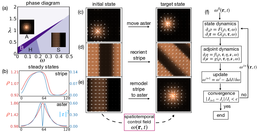
The phenomenology of this model is described in [62] and summarized in Fig. 1a. For the purposes of this work, we note that the dynamics of this system admits two inhomogeneous steady states: (i) propagating stripes composed of ordered swarms moving through a disordered background, which are referred to as polar drops elsewhere in the literature [68, 63], when , and (ii) a stationary high density aster, again in an isotropic background, when . Both of these states arise close to the threshold density for orientational ordering (which we set to ), and correspond to the system phase separating into a dense ordered phase and a dilute disordered phase. In this study, we fix the homogeneous density at and consider the problem of controlling these inhomogeneous steady states using spatiotemporal patterning of the convective strength , referred to as the activity or control parameter in the rest of this paper.
This model has the virtue of mathematical simplicity and a minimal number of parameters, thus enabling physical insight from the optimal control solutions. At the same time, the states we seek to control are directly realizable in experiments (see section V). Further, in the SI [69], we show that this theory is linearly controllable on short length scales. Thus it is ideal for investigating applications of optimal control in active systems.
III OPTIMAL CONTROL
Spatiotemporal control of the system involves identifying an activity field in an interval such that the state of the system evolves from some initial condition , to a chosen target state , within the control window . We define this in terms of to constrain solutions to positive activity. In the optimal control framework, we identify such a solution by minimizing the scalar objective function defined as
| (5) |
subject to the constraints that the dynamical fields , obey Eq.(18) and Eq.(19) at every time point in the control window. The term penalizes deviations of the magnitude of the control variable from some baseline , and thereby discourages control solutions to be away from some chosen value of activity. The terms and promote smoothness of the activity field in space and time. To simplify the presentation of results, we set and thus do not penalize time-variations.
The terms and measure the deviations from the target state, and . We constrain our search of optimal state trajectories to those that obey the system dynamics by introducing Lagrange multipliers, and , which are adjoint variables for and . These dynamical constraints are enforced in the optimization by adding them to the cost function as
| (6) |
The necessary condition for optimality is [70, 71], so , , , , , , . The first two conditions return equations (18)-(19) governing and . The following two conditions yield the dynamical equations for the adjoint variables and ,
| (7) |
| (8) |
with boundary conditions at : , and periodic boundary conditions on the domain. yields an equation to update the control input as,
| (9) |
We use the direct-adjoint-looping (DAL) method [72] to minimize the cost function under the constraint that the dynamics satisfies Eqs. (18) and (19), to yield the optimal schedule of activity in space and time (see SI sections IV and V for more details). Specifically, we construct an initial condition by performing a simulation with unperturbed dynamics (Eqs. (18) and (19)) until reaching steady-state, at a parameter set that leads to a desired initial behavior. We construct a target configuration in the same manner, using a different parameter set that leads to the desired target behavior. We also specify a time duration over which the control protocol will be employed, and an initial trial control protocol. We then perform a series of DAL iterations; in each iteration the system and the adjoint dynamics are integrated from the initial condition for time under the current control protocol, and the cost function (Eq. (20)) is computed from the resulting trajectory. The adjoint equations are integrated backwards in time to propagate the residuals. After each backward run, the control protocol is updated via gradient descent, , to minimize the cost function. We employ Armijo backtracking [73] to adaptively choose the step-size for gradient descent and to ensure convergence of the DAL algorithm. We have implemented this calculation in the open-source Python finite element method solver FEniCS [74].
IV RESULTS
Using the optimal control framework described in section III and the hydrodynamic equations Eqs. (18) and (19), we have computed spatiotemporal control solutions that steer the system state toward the target configuration, for each of the target behaviors shown in Fig. 1 (c-e). In this section, we describe these calculations, and physical insights that can be learned by studying the computed control solutions.
IV.1 Aster advection
First, starting in a parameter regime where a stationary aster is stable ( and ), we seek to advect an aster to a new location. The control problem specifies the initial and final states of the system as well as the elapsed time; that is, the spatial dependence of the density and polarization fields at every point in space at times and .
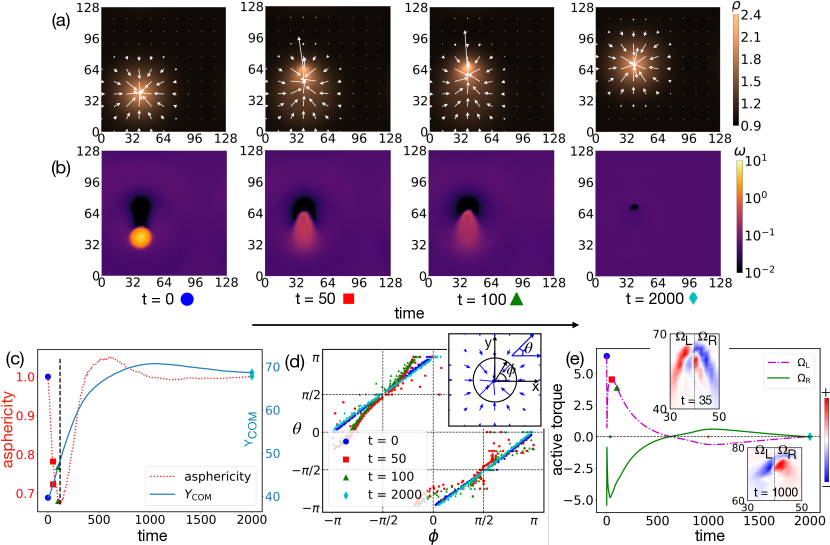
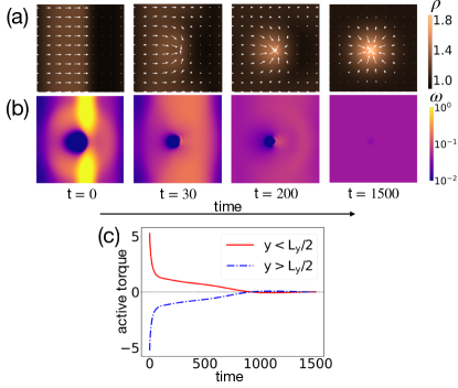
Fig. 2 summarizes the results of this computation. Fig. 2a,b respectively show the time evolution of the system configuration and the applied control field that drives the transformation. At early times, the applied control is strongest at the aster core while it is lowest in front of the aster along the direction we seek to move it. The aster then elongates to assume a comet-like shape, with a denser, polar-ordered head (see snapshots at ), as it advects toward the target location. Note that the activity is largest to the rear of the aster in this region. Thus, the control solution pushes (rather than pulls) the aster.
To quantify how the position and profile of the aster change over the course of advection, we measure its center-of-mass position and asphericity. Here, we track the y-coordinate of the center of mass, which is calculated as , and the asphericity is given by the ratio of eigenvalues of shape tensor: , where Latin indices denote grid points and Greek indices correspond to Cartesian coordinates, and is the distance of the grid point from the center of mass. As shown in Fig. 2c, the control window naturally partitions into two stages. During the initial stage () the aster rapidly changes shape into the comet-like configuration, as seen by the decrease in its asphericity, while simultaneously undergoing advection, moving towards the target point. Then, over the remaining long time window ( the aster reforms slowly, the asphericity increases back to 1, and it moves the remaining small distance to the target position.
For further description of the aster profile during these stages, we present the angle of the polarization field as a function of the azimuthal angle around the aster core at four time points in Fig. 2d. At the initial time () the system is radially symmetric with polarization vectors pointing toward the aster center, while by and the symmetry of in the top and bottom quadrants is broken, with more polarization at the bottom points toward the advection direction, and the front-end remains aster-like with a radial configuration. The orientation returns to the aster configuration by .
Further, we can understand the control solution physically by noting that the dynamics of is such that gradients in the control field create a torque on the orientation field, i.e., or equivalently . We then calculate the integral of the torque () over two domains, on the left and and to the right, with in our case (Fig. 2e). When the aster unwinds and advects, the region to the left has a positive torque (countercockwise rotation) and the region on the right experiences negative torque (clockwise rotation), which correspond to the partial unwinding of the aster. This is also illustrated by the snapshot shown for , where the dashed line () represents the axis along the aster’s motion. During the subsequent reformation phase, as the aster regains circular symmetry, the profile winds back such that the left/right subdomains experience clockwise/counterclockwise torque respectively. The snapshot shown at illustrates this behavior. Eventually, the system relaxes sufficiently close to an unperturbed aster configuration that the net torque becomes zero.
IV.1.1 Specifying the trajectory of aster advection
A limitation of the approach described thus far is that convergence of the control solution becomes unreliable when trying to advect the aster over distances significantly greater than its size (). This is because the gradients in the objective function are extremely shallow for the initial stages of the trajectory when the target state is far from the initial state. While techniques to find global minima can potentially overcome this problem, an alternative approach is to change the objective function to ensure sufficient gradients at all stages. A simple example of the latter strategy is to prescribe the entire trajectory of the aster. This approach has the added benefit of controlling the translocation speed, but has the potential drawback of arriving at a suboptimal solution (either slower translocation or higher control cost), since the problem is more constrained.
We applied the latter strategy to the problem of translocating an aster a distance of . We formulated the control problem to translocate the aster at a constant speed for a time , follow by a time for reformation of the aster. We find that specifying the path in this way allows specifying a target distance that is arbitrarily far without any difficulties in achieving convergence of the control solution.
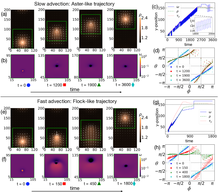
Figs. 3a,b show the system configurations and corresponding control solution for an example with , , and . At , the activity is maximum at the core of the aster, but unlike the previous setup where only initial and final state of the aster are specified, the order of magnitude remains same throughout the advection phase of aster. During the first phase of the solution (constant advection), the aster undergoes partial dissolution and, as intended, a roughly steady rate of translation toward the target (see snapshots at ). However, because we specified the trajectory at discrete intervals spaced by , the optimal control field oscillates with a period of about . This behavior is evident in Fig. 3c, which shows the positions of the maxima of and and the minimum of the y-component of the torque, , as a function of time. The maximum in the control solution exhibits strong oscillations of length units between the front and rear of the aster (while the activity remains low at the aster core, see Fig. 3b), whereas the density maximum moves at a nearly continuous speed toward the target. The minimum tracks polarization toward the direction and it consistently coincides with the high activity point at the front of the aster. Taken together, these observations show that the control solution pushes the aster from the rear, while exerting torques at the front that maintain aster-like polarization. This is captured in Fig. 3d which shows as a function of the azimuthal angle at two intermediate times during the advection phase, t= 1200 and 1900. Finally, during the second (reformation) phase, the aster re-acquires its radially symmetric steady state density and polarization profile. The dynamical interplay among these forces can be seen in the supplemental video [69].
Since we are specifying the path of the aster, we can investigate how the control solution depends on the chosen advection rate. Fig. 3e-h shows analogous results for a trajectory in which the advection phase is shortened to , forcing a higher translation speed . The higher speed leads to a qualitatively different type of trajectory; the aster unwinds into a flock during the advection phase, and then reforms during the second phase. Here the control solution takes a bean-shaped spatial profile, which initially pulsates periodically to unwind the leading edge of the aster and push the aster toward the target position. At early times (by ) the rear of the aster adopts a flock-like state with polarization primarily pointing in the direction; by most of the aster becomes flock-like. The extent of polarization along is particularly clear from the plot of at (Fig. 3h, green triangles).
These two control problems indicate that the specification of the cost function can result in very different activity profiles and intermediate states in the optimal solution. We can introduce other metrics and constraints to obtain solutions that are potentially more readily implementable in experiments.
IV.2 Changing the direction of propagating stripes.
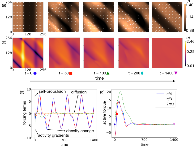
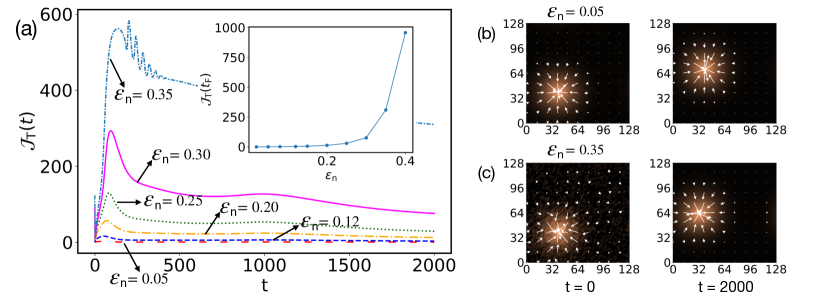
Next, starting at a parameter set for which stripes are stable, we obtain an activity profile to change the stripe propagation direction, with initial direction along and a target direction diagonally oriented along . Note that we obtain similar results for any target orientation, including reversing the stripe direction by . Fig. 4 a,b show the system configurations and corresponding control solutions at several time points. At , the applied activity is strongest at the leading edge of the stripe, and decays over the width of the leading boundary layer (i.e., the region where the polarization changes from isotropic to uniform). These gradients in activity lead to both melting (reduction of the magnitude of polarization) and turning (reorientation of polarization toward the target direction). At the next two time-points () the activity has decreased in magnitude, but continues to turn the polarization. By the activity is nearly uniform in space and approaching its steady-state value of 0.4. However, some curvature remains near the leading edge of the stripe. The stripe has completely reformed by the last time point (). Notably, the timescale for dissolving and reorienting the stripes at this periodic box size (SI Movie S4 [69]) was about in our dimensionless units, which is 2 orders of magnitude lower than obtaining stripes from a random homogenous initial condition in the absence of control.
While an intuitive route to reorienting a strip would be to melt the stripe to an isotropic domain and then have it reform in the new direction, this is not the optimal solution given by the control theory. Starting with the density equation, Eq.(18), we investigate the primary forces influencing density evolution during the stripe reorientation process. For this we choose a subdomain within the simulation box of size . We integrate each of the three terms in Eq.(18) over the specified subdomain as a function of time (Fig. 4c): , which governs the convection of active particles at convection speed ; , which determines the local density dynamics due to gradients in activity; and , which determines the diffusion due to density gradients. We find that, at all times, the dominant contribution arises from self-propulsion, ; contributions from gradients in activity and density have negligible contributions. Thus, we conclude that activity gradients are not the driving force for the density dynamics, but rather lead to the torques that reorient the polarization field, as described in our analysis in IV.1. To quantify the effect of active torque in this case, we illustrate in Fig 4c that as the difference in orientation between the initial state and target state increases, the active torque also increases, and as the system settles into the target orientation, the active torque goes to 0.
IV.3 Remodeling stripe to aster
So far, we have considered cases where the initial and target states are both steady states of the uncontrolled forward dynamics of our system at specified parameters. To demonstrate the power of the control theory, we start in a parameter regime in which propagating stripes are stable, and obtain an activity profile that drives the system into a stationary aster (not a steady state at these parameters). For the initial condition, we run to steady-state under parameters that lead to propagating stripes, and . To obtain a configuration to specify the target state, we perform an independent simulation in which we obtain a stationary aster steady-state with and . Fig. 5 shows the trajectory and corresponding control solution. We see that at early times the applied activity is strongest at the top- and bottom-edges of the leading boundary layer of the stripe, which bends the polarization vectors toward the core of the target aster. The magnitude of the activity field decreases quickly in time, but the spatial profile remains similar, thus continuing to steer polarization toward the core, and decreasing the net momentum in the direction. Due to the coupling between and (see Eq. (18)), the resulting gradients and polarization lead to convection of density toward the core. By , there is a density maximum at the core and the system has achieved a radially symmetric state, which leads to a balance of propulsion forces and thus a stationary state.
IV.4 Robustness of optimal control solution to noise.
Since models are never completely accurate and noise is inevitable in any experimental system, we investigated the robustness of our control solution to errors or noise. Because our implementation uses deterministic PDEs, we tested the effects of noise by perturbing the initial condition for the aster translocation problem presented in Fig. 2. Specifically, we added Gaussian noise with a relative magnitude to the values and at each pixel, and then integrated the dynamics with the control protocol computed in the absence of noise. Fig. 6 shows the performance of the control solution. We plot the deviation from the target state, , and the inset shows the deviation of the final state from the target , as a function of . We see that noise has a relatively small effect on the performance up to a magnitude of about , after which deviations in the objective function rise dramatically. However, even with and a relatively large value of at , the final state is remarkably close to the target in all qualitative aspects (see Fig. 6c), with a well-formed aster close to the target position. Thus, we conclude that the optimal control solution is robust to noise, at least in the initial condition.
V Discussion and conclusions
We demonstrate an optimal control theory framework that can prescribe activity patterns to guide an active material into desired emergent behaviors, focusing on an active polar fluid as a model system. The capabilities include programmed switching among dynamical attractors with very different dynamics and distinct broken symmetry patterns, and reprogramming the dynamics of existing attractor states. As an example of the former, we identify a spatiotemporal activity pattern that converts a propagating stripes state into a stationary aster. As an example of the latter, we show that a stationary aster can be programmed to self-advect to a new target configuration, either via an arbitrary trajectory or along a prescribed path. Similarly, propagating stripes can be forced to reorient in arbitrary directions. Depending on the choice of terms and weights in the objective function, the spatiotemporal variations of the control inputs can be regulated to limit experimental cost or ensure smooth trajectories.
Further, we show that the optimal control solutions are robust to noise. In particular, perturbing the initial condition by up to 20% leads to minimal quantitative deviations from the target behavior, and the solution remains qualitatively accurate for significantly larger perturbations. Also, we note that additional strategies can be employed for experimental systems where larger noise sources or systematic errors are unavoidable. This includes integrating closed-loop control components. For example, one can observe the current state of the system at regular intervals along a trajectory, and recompute the optimal control solution using the current state as the initial condition. Alternatively, one can add linear feedback terms that analyze deviations from the pre-computed optimal control trajectory [75].
In addition to directly applying the computed activity protocols, examination of their forms provides both fundamental and practical insights into controlling active materials. In particular, we show how the spatial gradients in the applied activity field lead to localized torques which rotate polarization directions, leading to the programmed reformulation of the pattern of interest (e.g. aster or stripe). Unsurprisingly, the form of the trajectory is different depending on the task being encoded for — changing the broken symmetry state of the system (e.g. stripe-to-aster, Fig. 5) requires very different spatial arrangements of active torques then advection (Figs. 2 and 3) or reorientation (Fig. 4). Notably however, the applied activity field and corresponding trajectory also depend strongly on the time allowed for the transformation. In the example of advecting the aster over a distance many times its size (Fig. 3), the aster mostly retains its form throughout the course of the trajectory when moving at moderate speed, but when forced to complete the journey faster, the applied activity field reshapes the aster into a localized flock or swarm, which reformulates into an aster upon reaching the target position.
The states we seek to control are realizable in experiments. Propagating concentration waves of aligned self-propelled particles have been observed in dense actin motility assays [76, 77, 78, 79] and in self-chemotactic bacterial systems[80, 81, 82, 83, 84, 85, 86, 87, 88] . Asters are ubiquitous in cell biology in processes such as the formation of the mitotic spindle, oogenesis, and plant cell cytokinesis. [89, 90, 91, 92, 93, 94, 95, 96]. They can be reliably obtained in in vitro suspensions of cytoskeletal filaments and motor proteins[92, 6, 97, 98, 99, 100, 101, 102, 103, 104, 105, 106, 107, 46]. In such systems, activity can be controlled in space and time by constructing active materials with optogenetic molecular motors, and using a digital light projector to shine a programmed spatiotemporal sequence of light on the sample [43, 44, 45, 46]. Thus, our results can be directly tested.
The optimal control framework presented here is highly generalizable, and can be readily applied to any system provided there is a means to externally actuate the system and there is a reasonably accurate continuum model. Importantly, the control variable need not be limited to the activity field, since the objective function can be extended to include any property of the material that can be actuated. With the recent success of automated PDE learning tools in discovering continuum models for active systems (e.g. [108, 109, 110]), applications need not be limited to systems with accurate models already available. Furthermore, since model discovery tools work better when provided with a variety of data, including from non-steady-state observations, we anticipate that combining model discovery tools with optimal control could be a powerful approach to both discover more accurate models and enhance the reliability of the control solutions.
Acknowledgements.
This work was supported by the Department of Energy (DOE) DE-SC0022291. Preliminary data and analysis were supported by the National Science Foundation (NSF) DMR-1855914 and the Brandeis Center for Bioinspired Soft Materials, an NSF MRSEC (DMR-2011846). Computing resources were provided by the NSF XSEDE allocation TG-MCB090163 (Stampede and Expanse) and the Brandeis HPCC which is partially supported by the NSF through DMR-MRSEC 2011846 and OAC-1920147. AB acknowledges support from NSF-2202353.References
- Liu and Lin [2012] K.-A. Liu and I. Lin, Physical Review E 86, 011924 (2012).
- Czirók and Vicsek [2000] A. Czirók and T. Vicsek, Physica A: Statistical Mechanics and its Applications 281, 17 (2000).
- Pierce et al. [2018] C. Pierce, H. Wijesinghe, E. Mumper, B. Lower, S. Lower, and R. Sooryakumar, Physical Review Letters 121, 188001 (2018).
- Needleman and Dogic [2017] D. Needleman and Z. Dogic, Nature reviews materials 2, 1 (2017).
- Sarfati et al. [2022] G. Sarfati, A. Maitra, R. Voituriez, J.-C. Galas, and A. Estevez-Torres, Soft Matter 18, 3793 (2022).
- Ndlec et al. [1997] F. Ndlec, T. Surrey, A. C. Maggs, and S. Leibler, Nature 389, 305 (1997).
- Surrey et al. [2001] T. Surrey, F. Nédélec, S. Leibler, and E. Karsenti, Science 292, 1167 (2001).
- Gardel et al. [2008] M. L. Gardel, K. E. Kasza, C. P. Brangwynne, J. Liu, and D. A. Weitz, Methods in cell biology 89, 487 (2008).
- Gardel et al. [2010] M. L. Gardel, I. C. Schneider, Y. Aratyn-Schaus, and C. M. Waterman, Annual review of cell and developmental biology 26, 315 (2010).
- Dogterom and Koenderink [2019] M. Dogterom and G. H. Koenderink, Nature reviews Molecular cell biology 20, 38 (2019).
- Soares e Silva et al. [2011] M. Soares e Silva, M. Depken, B. Stuhrmann, M. Korsten, F. C. MacKintosh, and G. H. Koenderink, Proceedings of the National Academy of Sciences 108, 9408 (2011).
- Wagner et al. [2022] C. G. Wagner, M. M. Norton, J. S. Park, and P. Grover, Physical Review Letters 128, 028003 (2022).
- Wang et al. [2015] W. Wang, W. Duan, S. Ahmed, A. Sen, and T. E. Mallouk, Accounts of chemical research 48, 1938 (2015).
- Gomez-Solano et al. [2017] J. R. Gomez-Solano, S. Samin, C. Lozano, P. Ruedas-Batuecas, R. van Roij, and C. Bechinger, Scientific reports 7, 14891 (2017).
- Hallatschek et al. [2023] O. Hallatschek, S. S. Datta, K. Drescher, J. Dunkel, J. Elgeti, B. Waclaw, and N. S. Wingreen, Nature Reviews Physics , 1 (2023).
- Liu et al. [2021] S. Liu, S. Shankar, M. C. Marchetti, and Y. Wu, Nature 590, 80 (2021).
- Hamby et al. [2018] A. E. Hamby, D. K. Vig, S. Safonova, and C. W. Wolgemuth, Science advances 4, eaau0125 (2018).
- Ni et al. [2020] B. Ni, R. Colin, H. Link, R. G. Endres, and V. Sourjik, Proceedings of the National Academy of Sciences 117, 595 (2020).
- Lauga and Powers [2009] E. Lauga and T. R. Powers, Reports on progress in physics 72, 096601 (2009).
- Gonzalez-Rodriguez et al. [2012] D. Gonzalez-Rodriguez, K. Guevorkian, S. Douezan, and F. Brochard-Wyart, Science 338, 910 (2012).
- Henkes et al. [2020] S. Henkes, K. Kostanjevec, J. M. Collinson, R. Sknepnek, and E. Bertin, Nature communications 11, 1405 (2020).
- Fodor and Marchetti [2018] É. Fodor and M. C. Marchetti, Physica A: Statistical Mechanics and its Applications 504, 106 (2018).
- Nichol and Khademhosseini [2009] J. W. Nichol and A. Khademhosseini, Soft matter 5, 1312 (2009).
- Zhang et al. [2020] G. Zhang, R. Mueller, A. Doostmohammadi, and J. M. Yeomans, Journal of the Royal Society Interface 17, 20200312 (2020).
- Doostmohammadi et al. [2016] A. Doostmohammadi, S. P. Thampi, and J. M. Yeomans, Physical review letters 117, 048102 (2016).
- Saw et al. [2017] T. B. Saw, A. Doostmohammadi, V. Nier, L. Kocgozlu, S. Thampi, Y. Toyama, P. Marcq, C. T. Lim, J. M. Yeomans, and B. Ladoux, Nature 544, 212 (2017).
- Trepat et al. [2009] X. Trepat, M. R. Wasserman, T. E. Angelini, E. Millet, D. A. Weitz, J. P. Butler, and J. J. Fredberg, Nature physics 5, 426 (2009).
- Trepat and Sahai [2018] X. Trepat and E. Sahai, Nature Physics 14, 671 (2018).
- Duclos et al. [2014] G. Duclos, S. Garcia, H. Yevick, and P. Silberzan, Soft matter 10, 2346 (2014).
- Blanch-Mercader et al. [2018] C. Blanch-Mercader, V. Yashunsky, S. Garcia, G. Duclos, L. Giomi, and P. Silberzan, Physical review letters 120, 208101 (2018).
- Garcia et al. [2015] S. Garcia, E. Hannezo, J. Elgeti, J.-F. Joanny, P. Silberzan, and N. S. Gov, Proceedings of the National Academy of Sciences 112, 15314 (2015).
- Ghibaudo et al. [2008] M. Ghibaudo, A. Saez, L. Trichet, A. Xayaphoummine, J. Browaeys, P. Silberzan, A. Buguin, and B. Ladoux, Soft Matter 4, 1836 (2008).
- Vicsek and Zafeiris [2012] T. Vicsek and A. Zafeiris, Physics reports 517, 71 (2012).
- Chaté [2020] H. Chaté, Annual Review of Condensed Matter Physics 11, 189 (2020).
- Doostmohammadi et al. [2018] A. Doostmohammadi, J. Ignés-Mullol, J. M. Yeomans, and F. Sagués, Nature communications 9, 1 (2018).
- Bechinger et al. [2016] C. Bechinger, R. Di Leonardo, H. Löwen, C. Reichhardt, G. Volpe, and G. Volpe, Reviews of Modern Physics 88, 045006 (2016).
- Gompper et al. [2020] G. Gompper, R. G. Winkler, T. Speck, A. Solon, C. Nardini, F. Peruani, H. Löwen, R. Golestanian, U. B. Kaupp, L. Alvarez, et al., Journal of Physics: Condensed Matter 32, 193001 (2020).
- Marchetti et al. [2013] M. C. Marchetti, J.-F. Joanny, S. Ramaswamy, T. B. Liverpool, J. Prost, M. Rao, and R. A. Simha, Reviews of Modern Physics 85, 1143 (2013).
- Aubret et al. [2018] A. Aubret, M. Youssef, S. Sacanna, and J. Palacci, Nature Physics 14, 1114 (2018).
- Palacci et al. [2013] J. Palacci, S. Sacanna, A. P. Steinberg, D. J. Pine, and P. M. Chaikin, Science 339, 936 (2013).
- Arlt et al. [2018] J. Arlt, V. A. Martinez, A. Dawson, T. Pilizota, and W. C. Poon, Nature communications 9, 768 (2018).
- Frangipane et al. [2018] G. Frangipane, D. Dell’Arciprete, S. Petracchini, C. Maggi, F. Saglimbeni, S. Bianchi, G. Vizsnyiczai, M. L. Bernardini, and R. Di Leonardo, Elife 7, e36608 (2018).
- Lemma et al. [2023] L. M. Lemma, M. Varghese, T. D. Ross, M. Thomson, A. Baskaran, and Z. Dogic, PNAS nexus 2, pgad130 (2023).
- Zarei et al. [2023] Z. Zarei, J. Berezney, A. Hensley, L. Lemma, N. Senbil, Z. Dogic, and S. Fraden, Soft matter 19, 6691 (2023).
- Zhang et al. [2021] R. Zhang, S. A. Redford, P. V. Ruijgrok, N. Kumar, A. Mozaffari, S. Zemsky, A. R. Dinner, V. Vitelli, Z. Bryant, M. L. Gardel, et al., Nature Materials 20, 875 (2021).
- Ross et al. [2019] T. D. Ross, H. J. Lee, Z. Qu, R. A. Banks, R. Phillips, and M. Thomson, Nature 572, 224 (2019).
- Shankar et al. [2022] S. Shankar, L. V. Scharrer, M. J. Bowick, and M. C. Marchetti, arXiv preprint arXiv:2212.00666 (2022).
- Nasiri et al. [2023] M. Nasiri, H. Löwen, and B. Liebchen, Europhysics Letters 142, 17001 (2023).
- Knežević et al. [2022] M. Knežević, T. Welker, and H. Stark, Scientific Reports 12, 19437 (2022).
- Brunton and Kutz [2022] S. L. Brunton and J. N. Kutz, Data-driven science and engineering: Machine learning, dynamical systems, and control (Cambridge University Press, 2022).
- Dullerud and Paganini [2013] G. E. Dullerud and F. Paganini, A course in robust control theory: a convex approach, Vol. 36 (Springer Science & Business Media, 2013).
- Villani et al. [2009] C. Villani et al., Optimal transport: old and new, Vol. 338 (Springer, 2009).
- Norton et al. [2020] M. M. Norton, P. Grover, M. F. Hagan, and S. Fraden, Physical review letters 125, 178005 (2020).
- Sinigaglia et al. [2023] C. Sinigaglia, F. Braghin, and M. Serra, arXiv preprint arXiv:2305.00193 (2023).
- Toner and Tu [1995] J. Toner and Y. Tu, Physical review letters 75, 4326 (1995).
- Toner and Tu [1998] J. Toner and Y. Tu, Physical review E 58, 4828 (1998).
- Lee and Kardar [2001] H. Y. Lee and M. Kardar, Physical Review E 64 (2001), 10.1103/physreve.64.056113.
- Husain and Rao [2017] K. Husain and M. Rao, Physical Review Letters 118 (2017), 10.1103/physrevlett.118.078104.
- Geyer et al. [2018] D. Geyer, A. Morin, and D. Bartolo, Nature Materials 17, 789 (2018).
- Worlitzer et al. [2021] V. M. Worlitzer, G. Ariel, A. Be’er, H. Stark, M. Bär, and S. Heidenreich, New Journal of Physics 23, 033012 (2021).
- Mishra et al. [2010] S. Mishra, A. Baskaran, and M. C. Marchetti, Physical Review E 81 (2010), 10.1103/physreve.81.061916.
- Gopinath et al. [2012] A. Gopinath, M. F. Hagan, M. C. Marchetti, and A. Baskaran, Physical Review E 85, 061903 (2012).
- Caussin et al. [2014] J.-B. Caussin, A. Solon, A. Peshkov, H. Chaté, T. Dauxois, J. Tailleur, V. Vitelli, and D. Bartolo, Physical Review Letters 112 (2014), 10.1103/physrevlett.112.148102.
- Reinken et al. [2018] H. Reinken, S. H. L. Klapp, M. Bär, and S. Heidenreich, Physical Review E 97 (2018), 10.1103/physreve.97.022613.
- Ngamsaad and Suantai [2018] W. Ngamsaad and S. Suantai, Physical Review E 98 (2018), 10.1103/physreve.98.062618.
- Bertin et al. [2006] E. Bertin, M. Droz, and G. Grégoire, Physical Review E 74 (2006), 10.1103/physreve.74.022101.
- Peshkov et al. [2012] A. Peshkov, I. S. Aranson, E. Bertin, H. Chaté, and F. Ginelli, Physical Review Letters 109 (2012), 10.1103/physrevlett.109.268701.
- Solon and Tailleur [2013] A. P. Solon and J. Tailleur, Physical Review Letters 111 (2013), 10.1103/physrevlett.111.078101.
- [69] Supplemental Material: Spatiotemporal control of structure in a polar active fluid.
- Kirk [2004] D. E. Kirk, Optimal control theory: an introduction (Courier Corporation, 2004).
- Lenhart and Workman [2007] S. Lenhart and J. T. Workman, Optimal control applied to biological models (Chapman and Hall/CRC, 2007).
- Kerswell et al. [2014] R. Kerswell, C. C. Pringle, and A. Willis, Reports on Progress in Physics 77, 085901 (2014).
- Borzì and Schulz [2011] A. Borzì and V. Schulz, Computational optimization of systems governed by partial differential equations (SIAM, 2011).
- Dupont et al. [2003] T. Dupont, J. Hoffman, C. Johnson, R. C. Kirby, M. G. Larson, A. Logg, and L. R. Scott, The fenics project (Chalmers Finite Element Centre, Chalmers University of Technology, 2003).
- Bechhoefer [2021] J. Bechhoefer, Control Theory for Physicists (Cambridge University Press, 2021).
- Schaller et al. [2010] V. Schaller, C. Weber, C. Semmrich, E. Frey, and A. R. Bausch, Nature 467, 73 (2010).
- Huber et al. [2018] L. Huber, R. Suzuki, T. Krüger, E. Frey, and A. Bausch, Science 361, 255 (2018).
- Sciortino and Bausch [2021] A. Sciortino and A. R. Bausch, Proceedings of the National Academy of Sciences 118, e2017047118 (2021).
- Suzuki and Bausch [2017] R. Suzuki and A. R. Bausch, Nature communications 8, 41 (2017).
- Saragosti et al. [2011] J. Saragosti, V. Calvez, N. Bournaveas, B. Perthame, A. Buguin, and P. Silberzan, Proceedings of the National Academy of Sciences 108, 16235 (2011).
- Pohl and Stark [2014] O. Pohl and H. Stark, Physical review letters 112, 238303 (2014).
- Bhattacharjee et al. [2022] T. Bhattacharjee, D. B. Amchin, R. Alert, J. A. Ott, and S. S. Datta, Elife 11, e71226 (2022).
- Alert et al. [2022] R. Alert, A. Martínez-Calvo, and S. S. Datta, Physical review letters 128, 148101 (2022).
- Narla et al. [2021] A. V. Narla, J. Cremer, and T. Hwa, Proceedings of the National Academy of Sciences 118, e2105138118 (2021).
- Cremer et al. [2019] J. Cremer, T. Honda, Y. Tang, J. Wong-Ng, M. Vergassola, and T. Hwa, Nature 575, 658 (2019).
- Bhattacharjee et al. [2021] T. Bhattacharjee, D. B. Amchin, J. A. Ott, F. Kratz, and S. S. Datta, Biophysical Journal 120, 3483 (2021).
- Brenner et al. [1998] M. P. Brenner, L. S. Levitov, and E. O. Budrene, Biophysical journal 74, 1677 (1998).
- Fei et al. [2020] C. Fei, S. Mao, J. Yan, R. Alert, H. A. Stone, B. L. Bassler, N. S. Wingreen, and A. Košmrlj, Proceedings of the National Academy of Sciences 117, 7622 (2020).
- Mayer et al. [1999] T. U. Mayer, T. M. Kapoor, S. J. Haggarty, R. W. King, S. L. Schreiber, and T. J. Mitchison, Science 286, 971 (1999).
- Schaffner and José [2006] S. C. Schaffner and J. V. José, Proceedings of the National Academy of Sciences 103, 11166 (2006).
- Loughlin et al. [2010] R. Loughlin, R. Heald, and F. Nédélec, Journal of cell biology 191, 1239 (2010).
- Shirasu-Hiza et al. [2004] M. Shirasu-Hiza, Z. E. Perlman, T. Wittmann, E. Karsenti, and T. J. Mitchison, Current biology 14, 1941 (2004).
- Heidemann and Kirschner [1975] S. R. Heidemann and M. W. Kirschner, The Journal of cell biology 67, 105 (1975).
- Heidemann and Kirschner [1978] S. R. Heidemann and M. W. Kirschner, Journal of Experimental Zoology 204, 431 (1978).
- Schmit et al. [1983] A.-C. Schmit, M. Vantard, J. De Mey, and A.-M. Lambert, Plant cell reports 2, 285 (1983).
- Kumagai and Hasezawa [2001] F. Kumagai and S. Hasezawa, Plant biology 3, 4 (2001).
- Najma et al. [2024] B. Najma, W.-S. Wei, A. Baskaran, P. J. Foster, and G. Duclos, Proceedings of the National Academy of Sciences 121, e2300174121 (2024).
- Wollrab et al. [2019] V. Wollrab, J. M. Belmonte, L. Baldauf, M. Leptin, F. Nédeléc, and G. H. Koenderink, Journal of cell science 132, jcs219717 (2019).
- Foster et al. [2015] P. J. Foster, S. Fürthauer, M. J. Shelley, and D. J. Needleman, Elife 4, e10837 (2015).
- Colin et al. [2018] A. Colin, P. Singaravelu, M. Théry, L. Blanchoin, and Z. Gueroui, Current Biology 28, 2647 (2018).
- Luo et al. [2013] W. Luo, C.-h. Yu, Z. Z. Lieu, J. Allard, A. Mogilner, M. P. Sheetz, and A. D. Bershadsky, Journal of Cell Biology 202, 1057 (2013).
- Stam et al. [2017] S. Stam, S. L. Freedman, S. Banerjee, K. L. Weirich, A. R. Dinner, and M. L. Gardel, Proceedings of the National Academy of Sciences 114, E10037 (2017).
- Berezney et al. [2022] J. Berezney, B. L. Goode, S. Fraden, and Z. Dogic, Proceedings of the National Academy of Sciences 119, e2115895119 (2022).
- Thoresen et al. [2011] T. Thoresen, M. Lenz, and M. L. Gardel, Biophysical journal 100, 2698 (2011).
- Köster et al. [2016] D. V. Köster, K. Husain, E. Iljazi, A. Bhat, P. Bieling, R. D. Mullins, M. Rao, and S. Mayor, Proceedings of the National Academy of Sciences 113, E1645 (2016).
- Glaser et al. [2016] M. Glaser, J. Schnauß, T. Tschirner, B. S. Schmidt, M. Moebius-Winkler, J. A. Käs, and D. M. Smith, New Journal of Physics 18, 055001 (2016).
- Nédélec et al. [2003] F. Nédélec, T. Surrey, and E. Karsenti, Current opinion in cell biology 15, 118 (2003).
- Joshi et al. [2022] C. Joshi, S. Ray, L. M. Lemma, M. Varghese, G. Sharp, Z. Dogic, A. Baskaran, and M. F. Hagan, Physical review letters 129, 258001 (2022).
- Supekar et al. [2023] R. Supekar, B. Song, A. Hastewell, G. P. Choi, A. Mietke, and J. Dunkel, Proceedings of the National Academy of Sciences 120, e2206994120 (2023).
- Golden et al. [2023] M. Golden, R. O. Grigoriev, J. Nambisan, and A. Fernandez-Nieves, Science Advances 9, eabq6120 (2023).
Appendix A Moment of Inertia
The moment of inertia matrix for the aster is given by
| (10) |
with a mask to restrict the calculation to the vicinity of the aster:
| (11) |
where is the Heaviside step function and is the density field. That is, is the density field value at all points with density above the mean value; otherwise . The aster’s center of mass is dynamically tracked, and represents the distance of the -th point from the -th axis, which passes through aster’s center of mass.
Upon diagonalizing this moment of inertia matrix, we obtain the eigenvalues and , which correspond to the principal moments of inertia. We then define the asphericity as the ratio , which quantifies the extent of non-sphericity (asphericity) of the moving object.
A ratio closer to 1 indicates a more spherical shape, while significantly deviating values suggest an elongated or flattened form.
Appendix B Orientation field
We further quantify the motion of aster by measuring the orientation of polarization vectors relative to the polar axis. The reference point of the polar axis is determined by the point where density field has the maximum value. Our region of interest is a circular region of radius (in non-dimensional units), which is roughly the radius of an aster. We mask out the remaining space. This is depicted in the inset to Figure 2 in the main text, where the circle approximates the aster.
Appendix C Analyzing the optimal control solution: calculating the torque
We start with the full hydrodynamic equation for polarization:
| (12) |
During the initial stages, the applied activity profile exhibits large spatial gradients, with the predominant contribution to polarization dynamics largely stemming from the term :
| (13) |
We express , and re-write equation (13) as:
| (14) |
Further simplification yields:
| (15) |
| (16) |
Finally, this formulation results in:
| (17) |
where the expression (17) elucidates the temporal evolution of influenced by the cross product of the gradient of activity and the unit vector in the direction of the torque , normalized by the magnitude of .
Appendix D Direct-adjoint-looping (DAL) method
We use direct-adjoint-looping (DAL), an iterative optimization method [72] to solve for optimal schedule of activity in space and time that accomplishes our control goals. We start by writing the Lagrangian of optimization, Eq. (20), where and act as Lagrange multipliers or adjoint variables that constrain the dynamics to follow Eqs. (18) and (19).
We construct an initial condition by performing a simulation with unperturbed dynamics (Eqs. (18) and (19)) until reaching steady-state, at a parameter set that leads to a desired initial behavior. We construct a target configuration in the same manner, using a different parameter set that leads to the desired target behavior. We also specify a time duration over which the control protocol will be employed, and an initial trial control protocol . We then perform a series of DAL iterations, with each iteration involving the following steps:
- •
- •
-
•
Step 3: The control protocol is updated via gradient descent, , to minimize the cost function.
Iterations are continued until the gradient falls below a user-defined tolerance. We employ Armijo backtracking [73] to adaptively choose the step-size for gradient descent and to ensure convergence of the DAL algorithm.
Appendix E Derivation of Adjoint Equations
We begin with the equation of motion for the state variables:
| (18) |
| (19) |
We write the full objective function, which is the sum of terminal state and running state penalties that we aim to minimize, as follows:
where,
| (20) |
We then introduce Lagrange multipliers and that constrain the dynamics to the equations of motion for density and polarization respectively, and write the Lagrangian as:
| (21) |
The necessary condition for optimality is [70, 71], so , , , , , , and . The first two conditions of optimality yield back the dynamics equations. The next two conditions, , , yield dynamics equations for the adjoint variables and as:
| (22) |
| (23) |
with a boundary condition at time set by , as and . For our computations, we choose for simplicity since we obtained adequate convergence from the time-integrated penalty.
Finally, the condition yields:
| (24) |
which is used to update the control variable during gradient descent.
Appendix F Controllability
Let us consider the problem we want to solve in control theory. If we define , we seek to solve the set of nonlinear partial differential equations for the control solution , subject to a given initial condition , and a boundary condition in time , which is the target state with as the control window. A particular dynamical system is considered controllable if we can demonstrate the existence of a solution to the above problem. When the dynamics is nonlinear, demonstrations of controllability have been limited to a few simple systems where the nonlinearities have special properties. What we do instead is consider the controllability of Eqs. 18 -19 when linearized about the unstable fixed point of a homogeneous polar state. Demonstrating controllability of the homogeneous fixed point tells us that at short enough length scales, we will be able to drive the system to desired values of the dynamical fields, which can be thought of as different fixed points in the continuous space of fixed points associated with translational symmetry and broken rotational symmetry characteristic of our system.
Linearizing our theory using and , and introducing the Fourier transform, , we obtain
where denote the wavevectors along and orthogonal to direction of polarization, , and . Note that for all .
Let us now introduce the notation
, and
Our linearized theory is then of the form,
One can readily establish that this linear system has a solution to the boundary value control problem when the controllability matrix
is of rank 3 [50].
Computing the column vectors of , we obtain
To examine the rank of the matrix in a physically informative way, let us consider 3 special cases. First, let us consider the case of spatial gradients orthogonal to the direction of order. Setting and truncating the matrix elements to quadratic order in we obtain
As is apparent from the form of the matrix, the three column vectors are indeed linearly independent and hence the linearized theory of an active polar fluid is controllable in the presence of gradients in the direction perpendicular to that of the spontaneously broken symmetry. Next, let us consider two cases that show the limits on the controllability of the linear theory. If we consider the long wavelength limit of the controllability matrix , we see that, when truncated to lowest order in wavevector
which clearly is not of rank 3. Thus, the system is not controllable on the longest length scales. To identify the length scale up to which the system is controllable, let us compare the relevant terms in the second column. We will need to retain terms to quadratic order in the gradients when . Setting aside the direction of spatial homegeneity we get an estimate of the length scale up to which the system is controllable as . Given that all the terms on the right hand side scale with the mean density , the length scale up to which the linear system is controllable is set by the strength of the nonlinearities . Recall that our system is non-dimensionalized using the diffusive length scale and has the units of a diffusion coefficient. So, our system is controllable on length scales that are comparable to the diffusive length scale.
Finally, note that when we restrict attention to spatial gradients that lie purely along the direction of broken symmetry, the controllability matrix becomes
and the system is clearly not controllable. Thus, we see that spatial gradients orthogonal to the direction of the local polar order are critical to obtaining control solutions for an active polar fluid.
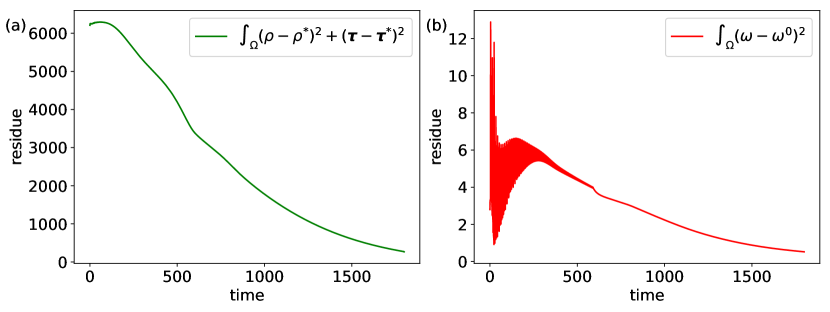
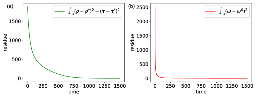
Appendix G Residues: deviations from target state as a function of time
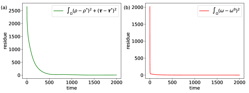
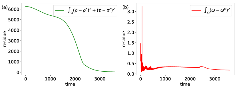
In this section, we assess how quickly the solutions approach their target by plotting the residues, meaning the deviations from the target state, , and the deviation of the control variable from its baseline value, . SI Figs. 7 – 10 show these residues as a function of time for the examples of: aster advection (Fig. 2 main text), aster advection with the trajectory specified (Figs.3a, 3b main text), and remodelling a stripe into an aster (Fig. 5 main text).
Appendix H Movie Descriptions
-
•
Movie S1: Aster translocation and reformation in the case where only the final state of the aster is specified (Fig. 2 main text). The left panel depicts density (color map) and polarization (arrows) profiles. The right panel shows the activity field , with a logarithmic scale colorbar.
-
•
Movie S2: Aster translocation and reformation where the trajectory of aster is specified, with slow advection (Aster-like trajectory, Fig. 3a main text). The left panel depicts density (color map) and polarization (arrows) profiles. The right panel shows the activity field , with a logarithmic scale colorbar.
-
•
Movie S3: Aster translocation and reformation where the trajectory of aster is specified, with fast advection (Flock-like trajectory, Fig. 3b main text).. The left panel depicts density (color map) and polarization (arrows) profiles. The right panel shows the activity field , with a logarithmic scale colorbar.
-
•
Movie S4: Reorienting the direction of propagation of a stripe by (Fig. 4 main text). The left panel depicts density (color map) and polarization (arrows) profiles. The right panel shows the activity field , with a logarithmic scale colorbar.
-
•
Movie S5: Remodelling a propagating stripe to a stationary aster (Fig. 5 main text). The left panel depicts density (color map) and polarization (arrows) profiles. The right panel shows the activity field , with a logarithmic scale colorbar.
-
•
Movie S6: Reorienting the direction of propagation of a stripe by . The left panel depicts density (color map) and polarization (arrows) profiles. The right panel shows the activity field , with a logarithmic scale colorbar.