Can Better Text Semantics in Prompt Tuning Improve VLM Generalization?

Abstract

Going beyond mere fine-tuning of vision-language models (VLMs), learnable prompt tuning has emerged as a promising, resource-efficient alternative. Despite their potential, effectively learning prompts faces the following challenges: (i) training in a low-shot scenario results in overfitting, limiting adaptability and yielding weaker performance on newer classes or datasets; (ii) prompt-tuning’s efficacy heavily relies on the label space, with decreased performance in large class spaces, signaling potential gaps in bridging image and class concepts. In this work, we ask the question if better text semantics can help address these concerns. In particular, we introduce a prompt-tuning method that leverages class descriptions obtained from large language models (LLMs). Our approach constructs part-level description-guided views of both image and text features, which are subsequently aligned to learn more generalizable prompts. Our comprehensive experiments, conducted across 11 benchmark datasets, outperform established methods, demonstrating substantial improvements.

1 Introduction

Foundational Vision-Language Models (VLMs) like CLIP [29] and ALIGN [12] have displayed remarkable zero-shot and open-vocabulary capabilities in recent times. This has led to VLMs being employed in various vision-only downstream tasks such as open-vocabulary image classification [19], object detection [7], and image segmentation [22]. Trained on extensive web data, these models most often use a contrastive loss to align image-text pairs in a shared embedding space, allowing them to represent diverse concepts.

Recently, learnable prompt-tuning [41, 16, 5] has emerged as a promising parameter efficient alternative for fine-tuning foundation models. Such prompt-tuning methods introduce learnable prompt vectors to tailor VLMs for specific tasks without affecting the pre-trained parameters of the VLM. While prompt-tuning methods have shown great promise, efficiently learning prompt vectors faces the following challenges: (i) training such prompts in a low-shot setting leads to overfitting, hindering their generalizability, and exhibiting sub-optimal performance when applied to newer classes or datasets [34, 16, 15], (ii) the performance of prompt-tuning methods can be highly dependent on the label space in which they operate. During inference, if the label space is large, the performance tends to decrease (see empirical evidence in § 5) due to bias towards the seen classes the model was fine-tuned on. This hints at a lack of understanding of images and categories in terms of their constituent concepts. This prods us to ask the question: can better text semantics in prompt tuning improve VLM generalization?

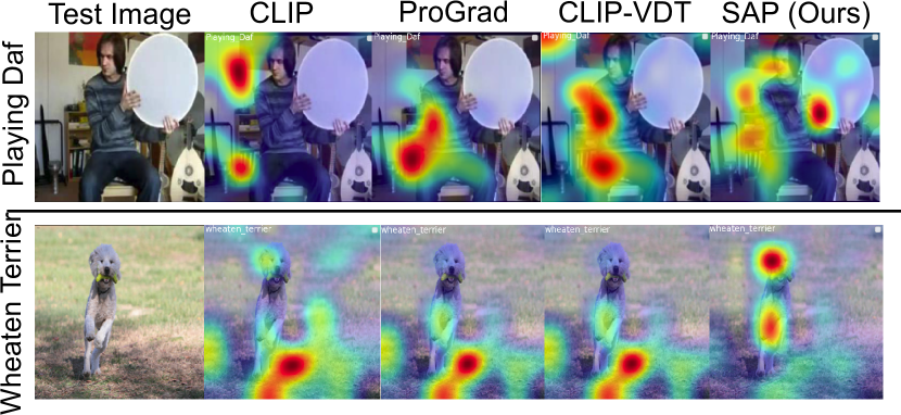
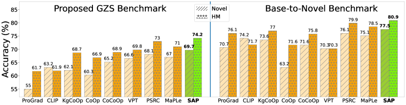
Figure 1: Left: Comparison of GradCAM [33] visualizations for our proposed method SAP against other baselines, on novel classes “Playing Daf” from an Action Recognition dataset [35] and “Wheaten Terrier” from Oxford Pets dataset [28]. The saliency maps indicate image regions that are most relevant to the descriptions “A photo of a person playing daf, with fingers hitting the drumhead” and “A photo of a wheaten terrier, which is wheat colored and has a square-shaped head” respectively. SAP effectively localizes the text semantics in images compared to baselines. Right: SAP surpasses other baselines on Generalized Zero-Shot (GZS) and Base-to-Novel (B2N) benchmarks, showing improvements of +1.6% and +1.2 on Novel Accuracy and Harmonic Mean (HM) for GZS, and +1.4% and +0.9 for B2N compared to best performing baseline.

Based on our studies in this direction, we propose SAP, Semantic Alignment for Prompt-tuning, which utilizes auxiliary text information in the form of easily obtained class descriptions to learn generalizable prompts. We however observe that mere use of such additional text semantics does not address the objective. Careful semantic alignment between image and text features, at different levels, plays an important role in leveraging such information. More specifically, given a set of class descriptions, we show how to construct class description-guided views of both image and text features. We then define semantic alignment as the average of similarities between corresponding views of image and text features. We use pre-trained Large Language Models (LLMs) to generate class descriptions in an inexpensive manner. A recent set of works [25, 39] has shown that class descriptions obtained from LLMs can be naively used to classify images on a given dataset with fixed categories. We go beyond and leverage these class descriptions to perform low-resource prompt-tuning, and show that such adapted VLMs show better generalization to unseen, novel classes. Fig. 1 illustrates the effectiveness of SAP over other baselines on two benchmarks, GZS and B2N (refer to § 5). Due to our part-level image-text alignment, SAP also showcases superior localization of visual concepts relevant to a class description, as seen through class activation maps, compared to other baselines including ones that use such auxiliary information (external knowledge) themselves.

Tab. 1 delineates the key differentiators of our approach compared to other baselines. Most existing prompt-tuning methods do not use such additional text semantics; even among the recent few that use such information, our method utilizes class descriptions at a part-level for both image and text. This strategy leads to non-trivial performance enhancements across benchmark datasets and improved localizations in novel classes or datasets. Additionally, we highlight a gap in the evaluation scheme used in existing prompt-tuning efforts, which demonstrate the performance of learned prompts primarily on the tasks of base-to-novel class generalization and cross-dataset evaluation. Inspired by the traditional Generalized Zero-Shot Learning (G-ZSL) [37, 20] paradigm, we posit that generalization in the zero-shot setting is more realistic when considering both base and novel classes at inference. We call this protocol GZS evaluation – the first such effort among prompt-tuning methods. We also propose another benchmark – Classification without class name – where the method is exclusively evaluated using class descriptions to classify images when its label lies outside CLIP’s vocabulary. To summarize our contributions:

• We propose a prompt-tuning method to fine-tune VLMs that can leverage class descriptions obtained from an LLM. Our novel approach to align class descriptions with image patch information allows us to utilize local features of an image, thus bridging image and text modalities using class descriptions.

• Our approach leverages auxiliary text semantics (class descriptions) to improve both image and text features in prompt-tuning for VLMs.

• We carry out a comprehensive suite of experiments with comparisons against state-of-the-art and very recent methods on standard benchmark datasets. We outperform existing baselines with a significant margin on all evaluation protocols.

• We propose two new evaluation protocols: GZS evaluation and classification without class name to better study the generalizability of prompt-tuning methods for VLMs. Our method consistently outperforms earlier baselines on these protocols, too.

	Text	Image	Use of External	Part-level	Evaluation	# of Additonal
Method	Prompts	Prompts	Knowledge	img-text	Benchmarks	Trainable
				alignment		Parameters
CoOp [41], CoCoOp [42], KgCoOp [40]	✓	✗	✗	✗	B2N, XDataset, DG	2k - 36k
ProGrad [43], ProDA [21]
MaPLe [15], PSRC [16],LoGoPrompt [34]	✓	✓	✗	✗	B2N, XDataset, DG	36k - 3.55M
KAPT [14], CoPrompt [32], CLIP-VDT [24]	✓	✓	✓	✗	B2N, XDataset, DG	1.3M - 4.74M
SAP (Ours)	✓	✓	✓	✓	GZS, B2N, XDataset, DG,	36K
					Classification w/o class names

Table 1: Comparison of the proposed method, SAP, with other related work on various key aspects involving Fine-tuning VLMs for better generalization. B2N: Base-to-Novel, XDataset: Cross Dataset, DG: Domain Generalization, GZS: Generalized Zero-Shot.

2 Related Work

Vision-Language Models. Vision-language models exhibit significant promise in acquiring generic visual representations. These models aim to harness natural language guidance for image representation learning and concurrently align both the text and image features within a shared embedding space. Conceptually, a vision-language model comprises three components: a text encoder, an image encoder, and a learning methodology that effectively utilizes information from both modalities. Recent research delves into establishing semantic connections between linguistic and visual elements, capitalizing on a vast reservoir of internet-based image-text pairs. For instance, CLIP [29] is the product of contrastive learning from 400 million carefully curated image-text pairs, while ALIGN [12] utilizes 1.8 billion noisy image-text pairs extracted from raw alt-text data. Nonetheless, a substantial challenge persists in transferring these foundational models to downstream tasks while preserving their initial capacity for generalization, which we aim to solve.

Prompt-Tuning. Prompt-tuning introduces task-specific text tokens designed to be learnable to customize the pre-trained VLM for downstream tasks. Context Optimization (CoOp) [41] marks the pioneering effort in replacing manually crafted prompts with adaptable soft prompts, fine-tuned on labeled few-shot samples. Conditional Context Optimization (CoCoOp) [42] builds upon this by generating image-specific contexts for each image and merging them with text-specific contexts for prompt-tuning. In contrast, Visual Prompt Tuning [13] introduces learnable prompts exclusively at the vision branch, resulting in sub-optimal performance for transferable downstream tasks. ProDA [21] focuses on learning the distribution of diverse prompts. KgCoOp [40] introduces regularization to reduce the discrepancy between learnable and handcrafted prompts, enhancing the generalizability of learned prompts to unseen classes. PSRC [16] shares a similar concept with KgCoOp [40] but introduces Gaussian prompt aggregation. ProGrad [43] selectively modifies prompts based on gradient alignment with general knowledge. MaPLe [15] introduces prompts at text and image encoder branches to strengthen coupling. In a distinct approach, LoGoPrompt [34] capitalizes on synthetic text images as effective visual prompts, reformulating the classification problem into a min-max formulation. All the existing methods focus on learning prompts but lack the ability to use class descriptions to capture finer contexts for better generalizability toward newer classes or datasets.

Use of External Knowledge A set of recent works [25, 39] provide evidence that visual recognition can be improved using concepts, and not just class names. However, [25] does not facilitate a way to perform fine-tuning on a downstream dataset. In contrast, [39] is a concept bottleneck model with a fixed label space and thus cannot be used for zero-shot classification. In fine-tuning methods incorporating external knowledge, KAPT [14] introduces complementary prompts to simultaneously capture category and context but lacks semantic alignment of each class description at the part-level of both image and text. On the other hand, CLIP-VDT [24] utilizes semantic-rich class descriptions only in the text modality, without semantic alignment with images. In a concurrent work CoPrompt[32], class descriptions are utilized via a regularizer acting as a consistency constraint to train the text prompts. There is no consideration of explicit semantic alignment with the image modality. Our approach utilizes class descriptions to semantically construct both text and image features, enhancing alignment between the two modalities. It helps unveil the hidden structures and promotes greater generalizability towards newer classes or datasets.

3 Preliminaries and Background

VLMs perform image classification on a downstream dataset by comparing an image representation with text representations of the class names in the dataset’s label space. When a small amount of labeled data is available, it has been shown that fine-tuning VLMs substantially boosts downstream performance [41, 42]. However, the fine-tuned model does not generalize to novel classes that were absent during fine-tuning [42]. In this work, we propose Semantic Alignment for Prompt Learning (SAP), that leverages class descriptions to fine-tune VLMs for better generalization to novel classes. Before we describe our methodology, we briefly discuss the required preliminaries, beginning with CLIP [29], the VLM chosen as our backbone following earlier work [41, 42, 15, 21, 40, 16, 43]. A summary of notations and terminology is presented in Appendix § 0.A.

CLIP Preliminaries. CLIP consists of an image encoder $\mathcal{I}$ and a text encoder $\mathcal{T}$, which are trained contrastively on paired image-text data to learn a common multi-modal representation space. $\mathcal{I}$ is typically a vision transformer [4] (we also show results with a ResNet [9]-based backbone, see Appendix § 0.D) and $\mathcal{T}$ is a transformer. $\mathcal{I}$ takes an image $\mathbf{x}\in\mathbb{R}^{C\times H\times W}$ as input and returns a $d$-dimensional feature vector. That is, $\mathbf{x}$ is divided into $M$ patches that are passed through the first layer of $\mathcal{I}$ to obtain patch tokens $\{\mathbf{e}_{1},\dots,\mathbf{e}_{M}\}$. A cls-token $\mathbf{cls}_{\mathcal{I}}$ is then added at the beginning of $\{\mathbf{e}_{1},\dots,\mathbf{e}_{M}\}$ to get $\{\mathbf{cls}_{\mathcal{I}},\mathbf{e}_{1},\dots,\mathbf{e}_{M}\}$. These tokens are passed through the transformer layers of $\mathcal{I}$. The $\mathbf{cls}_{\mathcal{I}}$ from the last layer undergoes a final projection to get an image feature vector $\mathbf{v}^{\mathbf{x}}$.

$\mathcal{T}$ processes a text string $S$ into a $d$-dimensional feature vector. The input text $S$ is tokenized into a sequence of $q$ word embeddings ${\mathbf{w}_{1},\dots,\mathbf{w}_{q}}$, appended with start and end tokens $\mathbf{w}_{s}$ and $\mathbf{w}_{e}$ respectively. The sequence ${\mathbf{w}_{s},\mathbf{w}_{1},\dots,\mathbf{w}_{q},\mathbf{w}_{e}}$ is then encoded by $\mathcal{T}$, producing the text feature vector $\mathbf{t}^{S}$. CLIP is trained with InfoNCE loss [27] to enhance cosine similarity for matching image-text pairs and to reduce it for non-matching pairs.

Zero-shot Classification using CLIP. CLIP performs zero-shot visual recognition of an image $\mathbf{x}$ by choosing the most similar class name from a set of candidate class names $\mathcal{Y}$, i.e., predicted class $\hat{y}=\operatorname*{arg\,max}\limits_{y\in\mathcal{Y}}sim(\mathbf{v}^{\mathbf{x}},\mathbf{t}^{y})$, where the similarity measure $sim$ is cosine-similarity. In practice, for a class name $y$, $\mathbf{t}^{y}$ is the text representation of a manually crafted prompt encapsulating $y$ such as ‘a photo of a [y]’. Zero-shot classification performance significantly depends on the label set $\mathcal{Y}$ considered, and can also vary with the template of the text prompt [29].

Fine-Tuning CLIP with Learnable Prompts. To perform efficient adaptation under limited supervision, prompt-tuning methods add a small number of learnable tokens to the input token sequence of either modality which are fine-tuned to generate task-specific representations. For instance, CoOp [41] adds $n$ learnable text-prompts $\mathcal{P}_{t}=\{\mathbf{p}_{1}^{t},\dots,\mathbf{p}_{n}^{t}\}$ to the input text token sequence $\{\mathbf{w}_{s},\mathbf{w}_{1},\dots,\mathbf{w}_{q},\mathbf{w}_{e}\}$. The final sequence $\{\mathbf{w}_{s},\mathbf{p}_{1}^{t},..,\mathbf{p}_{n}^{t},\mathbf{w}_{1},..,\mathbf{w}_{q},\mathbf{w}_{e}\}$ is passed through $\mathcal{T}$ to obtain the prompted text feature $\mathbf{t}_{p}(\mathcal{P}_{t})$. We follow IVLP [31], which adds learnable prompt tokens at transformer layers of both image and text encoders. That is, along with text prompts, IVLP appends learnable visual prompts $\mathcal{P}_{v}$ to image patch tokens, which are passed through $\mathcal{I}$ to yield the prompted visual feature $\mathbf{v}_{p}(\mathcal{P}_{v})$. Let $\theta=\{\mathcal{P}_{t},\mathcal{P}_{v}\}$ denote the set of all trainable text and visual prompts. These prompts are trained to maximize the similarity between a prompted image feature and the corresponding prompted text feature of its class name. Given $B$ image-text pairs $\{(\mathbf{x}_{i},y_{i})\}_{i=1}^{B}$, where $y_{i}\in\mathcal{Y}$, the likelihood of $\mathbf{x}_{i}$ predicting class $y_{i}$ is given by: $P_{\theta}(y_{i}\mid\mathbf{x}_{i})=\frac{\exp(s\cdot sim(\mathbf{v}_{p}^{\mathbf{x}_{i}}(\theta),\mathbf{t}_{p}^{y_{i}}(\theta)))}{\sum\limits_{y\in\mathcal{Y}}\exp(s\cdot sim(\mathbf{v}_{p}^{\mathbf{x}_{i}}(\theta),\mathbf{t}_{p}^{y}(\theta)))}$, where $s$ is the inverse temperature. The negative log-likelihood loss to be optimized is $L_{ce}(\theta)=\frac{-1}{B}\sum\limits_{i\in[B]}\log(P_{\theta}(y_{i}\mid\mathbf{x}_{i}))$.

With the above background, we now present our methodology to use class descriptions to learn prompts that can help VLMs generalize better to unseen, novel classes.

4 SAP: Methodology

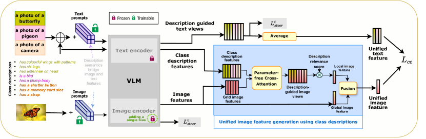
Figure 2: Our proposed workflow, SAP, performs part-based semantic alignment between image and text features. SAP integrates class descriptions into the text template and passed through the text encoder to construct description guided text views, which are then averaged to form a unified text feature. Global and grid image features are obtained from the image encoder. Description guided image views are obtained by performing parameter free cross-attention between class descriptor features and grid features. These image views are pooled into a local image feature, which is then fused with a global image feature to obtain the unified image feature. Unified text and image features contain part-level semantic information, and are aligned using a cross-entropy loss $L_{ce}$, and two steering losses $L_{steer}^{v}$, and $L_{steer}^{t}$.

Given labeled data, existing works learn prompts that largely limit themselves to incorporating class label-text information. We propose SAP, Semantic Alignment for Prompt-tuning, which utilizes auxiliary information in the form of class descriptions obtained from LLMs to learn more generalizable prompts. Our method constructs description guided text views and description guided image views that are aligned with each other. Conceptually, a class description provides a semantic context, and a description guided view is a feature conditioned on this context. We show how to construct such semantic-views for both image and text features using class descriptors. The alignment between image and text features is then simply the aggregate similarity between various semantic-views of the features. We term this robust, multidimensional alignment as semantic alignment. This external semantic knowledge, when integrated into the model, transfers to novel classes since the semantics are common concepts shared across multiple classes. The overview of our methodology is shown in Figure 2. We begin by describing how class descriptions are generated using LLMs.

4.1 Generating Class Descriptions

Large language models (LLMs) act as vast knowledge corpora that can be queried for the semantics of real-world objects. We use the popular LLM GPT-3.5 [8] to obtain textual descriptions for each class in a given dataset. Class descriptions commonly contain visual cues such as shape, texture, and color, as well as narratives of objects commonly correlated with the class. To keep our method cost-efficient, we use descriptions that are class-specific but not image-specific, thus making them reusable for a set of image samples. (Note that this is done only once per class label.) We use the responses from the LLM as they are, and do not manually curate or filter them any further. This keeps our approach low-cost while integrating finer semantic details into fine-tuning of VLMs. Some examples of our class descriptions are provided in Appendix § 0.E.

Class Description Features. For each class $y\in\mathcal{Y}$, where $\mathcal{Y}$ is the label space under consideration, we denote by $A_{y}$ the set of generated class descriptions. Let $A=\bigcup\limits_{y\in\mathcal{Y}}A_{y}$, $N=|A|$ denote the set of descriptions of all classes and the size of the set, respectively. Class description features $\mathbf{t}^{A}\in\mathbb{R}^{N\times d}$ are obtained by passing the class descriptions through $\mathcal{T}$. We denote class description features for class $y$ as $\mathbf{t}^{A_{y}}$. In the following sections, we describe how SAP leverages class descriptions and their feature representations to learn generalizable prompts.

4.2 Leveraging Class Descriptions for Text Features

The text feature $\mathbf{t}^{y}$ for a class $y\in\mathcal{Y}$ is generally obtained by encapsulating the class name in a text template and passing it through $\mathcal{T}$. We use aforementioned class descriptions $A_{y}$ to construct $\lvert A_{y}\rvert$ description guided views of this text feature. For a class description $a\in A_{y}$, the description guided text template for $y$ looks like: ‘a photo of a [y], which has [a]’ (e.g., ‘a photo of a cat, which has whiskers’). Learnable text prompts are then added to the above token sequence as described in § 3, which are passed through $\mathcal{T}$ to get the prompted, description guided view of class $y$ conditioned on $a$, $\mathbf{t}_{p}^{y,a}$. We denote the unprompted view as $\mathbf{t}^{y,a}$. The set of description guided text views of $y$ is denoted as $\mathbf{t}_{p}^{y,A_{y}}\in\mathbb{R}^{|A_{y}|\times d}$.

The various text views are averaged to generate a unified text feature, which is then utilized for image classification. Specifically, for class $y$, the unified text feature is $t_{pu}^{y}=\frac{1}{|A_{y}|}\sum_{a\in A_{y}}\frac{\mathbf{t}_{p}^{y,a}}{\lVert\mathbf{t}_{p}^{y,a}\rVert}$. The dot product between a normalized image feature $\frac{\mathbf{v}^{\mathbf{x}}}{\lVert\mathbf{v}^{\mathbf{x}}\rVert}$ and $\mathbf{t}^{y}_{pu}$ gives the average similarity w.r.t each view i.e, $\frac{\mathbf{v}^{\mathbf{x}}}{\lVert\mathbf{v}^{\mathbf{x}}\rVert}\cdot\mathbf{t}_{pu}^{y}=\frac{1}{\lvert A_{y}\rvert}\sum\limits_{a\in A_{y}}sim(\mathbf{v}^{\mathbf{x}},t_{p}^{y,a})$. Note that we take the average of normalized views to obtain the unified text feature. We validate our design choices in Tab. 6 by comparing against alternative ways to incorporate class descriptions.

4.3 Leveraging Class Descriptions for Image Features

As shown in Fig. 2, we also leverage the class descriptions in image representations through a Unified image feature generation module, where description-guided-views of an image are pooled into a class-agnostic local image feature. This local feature is then fused with the class-specific global image feature to form a unified image feature. We describe this process below.

Global and Grid Image Features. An image batch of size $B$ is passed through $\mathcal{I}$ (vision transformer) and the output of the final transformer block of shape $B\times(1+M+n)\times d^{\prime}$ is collected. Here, $1$ corresponds to the $\textbf{cls}_{\mathcal{I}}$ token, $M$ is the number of grid tokens, $n$ is the number of learnable prompt tokens, and $d^{\prime}$ is the dimension of the transformer layer. In all earlier works, including CLIP, the $\textbf{cls}_{\mathcal{I}}$ output token is passed through the final projection layer $proj\in\mathbb{R}^{d^{\prime}\times d}$ of $\mathcal{I}$ to obtain the global image features $\mathbf{V}_{g}\in\mathbb{R}^{B\times d}$. These features capture the global context of the image but may not capture local object-level semantics [30].

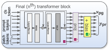
Figure 3: Addition of a bias vector to the last transformer block in $\mathcal{I}$

We aim to utilize the rich patch-level local information hidden in the $M$ grid tokens and establish their association with class descriptions. To obtain the grid image features $\mathbf{V}_{r}\in\mathbb{R}^{B\times M\times d}$, we pass the grid tokens through $proj$ and add a learnable $d$-dimensional bias offset as shown in the expanded $\mathcal{I}$ block in Fig. 3. This bias is added to fine-tune $proj$ with local information, which otherwise is used only to obtain global image features from the last transformer block. We represent the prompted global image features by $\mathbf{V}_{pg}$ and the prompted grid image features by $\mathbf{V}_{pr}$.

Constructing Description Guided Image Views using Grid Features. We use class description features $\mathbf{t}^{A}\in\mathbb{R}^{N\times d}$ together with prompted grid features of a given image $\mathbf{v}_{pr}\in\mathbb{R}^{M\times d}$ to construct $N$ description guided views for the image. To this end, we compute a parameter-free cross-attention with descriptor features as queries and grid features as keys and values. The cross-attention map $\mathbf{x}_{att}\in\mathbb{R}^{N\times M}$ between all descriptors (recall that $A$ is the union of all class-specific descriptions) and the grid features is:

$$\mathbf{x}_{att}=row\_softmax(\mathbf{t}^{A}\cdot\mathbf{v}_{pr}^{\intercal})\vspace{-4pt}$$

where the $i^{th}$ row of $\mathbf{x}_{att}$ gives the probability distribution of the alignment between the $i^{th}$ description and $M$ image patches. The description guided views of the image are then obtained by averaging the grid features using $\mathbf{x}_{att}$. Let $\hat{\mathbf{v}}_{pr}=\mathbf{x}_{att}\cdot\mathbf{v}_{pr}\in\mathbb{R}^{N\times d}$ denote the $N$ description guided views of the image. The $i^{th}$ row of $\hat{\mathbf{v}}_{pr}$ is a feature vector that describes the image in terms of the $i^{th}$ description i.e this semantic-view captures local visual phenomena pertinent to the $i^{th}$ description. Since descriptions are common across classes and even datasets, these features contain information that can transfer to novel classes.

Pooling Image Views into Local Image Features. The description guided view of grid features described above use class descriptions from all classes, and not just the ground-truth class of the image. Since the class descriptions generated by LLMs may be noisy, not all descriptions are relevant to a specific image. To address this, we introduce a description relevance score $\mathbf{r}\in[0,1]^{N}$, which quantifies each description’s similarity to the image. This is computed as $\mathbf{r}=softmax(\mathbf{v}_{pg}\cdot(\textbf{t}^{A})^{\intercal})$. To obtain a local representation of an image, we weigh each image view by its relevance score to compute a weighted mean of views. The local image feature $\mathbf{v}_{pl}\in\mathbb{R}^{d}$ thus captures finer contexts in an image and is computed as $\mathbf{v}_{pl}=\mathbf{r}\cdot\hat{\mathbf{v}}_{pr}$.

Fusing Global and Local Image Features. For an image, the global feature $\mathbf{v}_{pg}\in\mathbb{R}^{d}$ encodes class information pertaining to the image and the local feature $\mathbf{v}_{pl}\in\mathbb{R}^{d}$ encodes finer visual context. The final image feature is a fusion of the global and local features. We give a higher weight to the local score of an image if the descriptions attend strongly to specific grid patches of the image. For each description, the maximum attention weight over image patches is a proxy for the specificity of the description. We define the local score $l_{s}\in[0,1]$ as the weighted average of the maximum attention weight over the columns of $\mathbf{x}_{att}$. That is, $l_{s}=\mathbf{r}\cdot max(\mathbf{x}_{att},dim=1)$. We then weight the max-attention values using the relevance score; the final prompted unified image feature $\mathbf{v}_{pu}\in\mathbb{R}^{d}$ is an $l_{s}$-weighted combination of the global and local features defined as $\mathbf{v}_{pu}=(1-l_{s})\cdot\mathbf{v}_{pg}+l_{s}\cdot\mathbf{v}_{pl}$. We denote the prompted unified features for a batch of images as $\mathbf{V}_{pu}\in\mathbb{R}^{B\times d}$.

4.4 Aligning Prompted Image and Text Features

Given labeled data from a downstream dataset $\{(\mathbf{x}_{i},y_{i})\}_{i=1}^{B}$ with label space $\mathcal{Y}$, we obtain the prompted and unprompted unified image features, $\mathbf{V}_{pu}\in\mathbb{R}^{B\times d}$ and $\mathbf{V}_{u}\in\mathbb{R}^{B\times d}$ respectively, as described in § 4.3. For every class $y\in\mathcal{Y}$, description guided prompted and unprompted text features, $\mathbf{t}_{p}^{y,A_{y}}\in\mathbb{R}^{|A_{y}|\times d}$ and $\mathbf{t}^{y,A_{y}}\in\mathbb{R}^{|A_{y}|\times d}$ respectively, are obtained from $\mathcal{T}$. As outlined in § 3, we denote the set of all learnable text and visual prompts by $\theta$. Prompts are trained by minimizing the negative log-likelihood of the data:

$$\footnotesize L_{ce}(\theta)=-\frac{1}{B}\sum\limits_{i=1}^{B}\log\frac{\exp(s\cdot O_{\theta}(\mathbf{x}_{i},y_{i}))}{\sum\limits_{y\in\mathcal{Y}}\exp(s\cdot O_{\theta}(\mathbf{x}_{i},y))}\vspace{-2pt}$$

where $O_{\theta}(\mathbf{x}_{i},y)=\frac{1}{|A_{y}|}\sum_{a\in A_{y}}sim(\mathbf{v}_{pu}^{\mathbf{x}_{i}}(\theta),\mathbf{t}_{p}^{y,a}(\theta))$, $s$ is the scale (inverse temperature) parameter and logit $O(\mathbf{x},y)$ is the similarity between image $\mathbf{x}$ and class $y$. $sim(\mathbf{v}_{pu}^{x_{i}},\mathbf{t}_{p}^{y,a})$ is the similarity between the unified image feature and a single description guided text feature. We aggregate such similarities over all pertinent class descriptions and normalize by their count. A relevant description in the image enhances its similarity to the class; however, the absence of a description in the image does not penalize its similarity to the class. Following [40, 16], we add regularization terms designed to penalize prompted features that deviate significantly from their unprompted counterparts. We use the $L1$ penalty to regularize global image features and description guided text features.

$$\footnotesize L_{steer}^{v}(\theta)=\frac{1}{B}\sum\limits_{i=1}^{B}\lVert\mathbf{v}_{pg}^{\mathbf{x}_{i}}(\theta)-\mathbf{v}_{g}^{\mathbf{x}_{i}}\rVert_{1}\hskip 20.0ptL_{steer}^{t}(\theta)=\frac{1}{|\mathcal{Y}|}\sum\limits_{y\in\mathcal{Y}}\lVert\mathbf{t}_{p}^{y,A_{y}}(\theta)-\mathbf{t}^{y,A_{y}}\rVert_{1}$$

The final objective to optimize is: $\small{\mathcal{L}(\theta)=L_{ce}(\theta)+\lambda_{1}L_{steer}^{v}(\theta)+\lambda_{2}L_{steer}^{t}(\theta)}$, where $\lambda_{1}$ and $\lambda_{2}$ are hyperparameters.
Inference: Let $\mathcal{Y}^{\prime}$ be the inference time label space, and $A^{\prime}$ be the class descriptions of all classes in $\mathcal{Y}^{\prime}$. To predict the class of a test image $\mathbf{x}^{\prime}$, we compute the prompted unified image and text feature using the learned prompts, and compute logits as $O_{\theta}(\mathbf{x}^{\prime},y^{\prime})=\frac{1}{|A^{\prime}_{y}|}\sum_{a\in A^{\prime}_{y}}sim(\mathbf{v}_{pu}^{\mathbf{x}^{\prime}}(\theta),\mathbf{t}_{p}^{y^{\prime},a}(\theta))$. The class with highest score is predicted as the final label.

5 Experiments and Results

In this section, we comprehensively evaluate the generalization performance of SAP on four benchmark settings. (i) Generalized Zero-Shot (GZS) Benchmark: In this setting, the label space of a dataset is equally split into disjoint base and novel classes. Only a small number (16-shot) of labeled samples from the base classes are available as training data. However, during evaluation, the classification label space is the union of base and novel classes. As explained in § 3, zero-shot classification performance depends on the label set considered, and introducing base classes into the label space tests the bias of the fine-tuned model towards them. Though this setting has existed in traditional zero-shot learning [37], we introduce it back into the realm of VLMs. We believe this benchmark is a more realistic measure of the generalization performance of VLM fine-tuning methods. (ii) Base-to-Novel (B2N) Generalization: In this setting, followed by all prior work [41, 42, 15, 40, 16, 34], the dataset is split into equal disjoint base and novel classes, and the model is fine-tuned on few-shot (K=16) training split of the base classes. During evaluation, the label space is constrained to the set of classes (base or novel) the test image belongs to. The testing phase for B2N is thus separate for base and novel classes, whereas the GZS benchmark has a unified testing phase.(iii) Classification without Class Names (CwC): VLMs requires explicit class names to perform classification. This is a limitation for images whose label lies outside the VLM’s vocabulary. This benchmark tests the ability of a VLM to classify truly novel images without explicitly using the class-name. During inference, all class names are replaced with the word “object”, and the model is tested on it’s ability to classify an image based on descriptions alone. The model is fine-tuned on base classes, and evaluated on base and novel classes separately by replacing all class names. (iv) Cross-Dataset Generalization: In this setting, the model is fine-tuned on ImageNet [3] and tested on the remaining datasets. This measures the ability of a VLM fine-tuning method to generalize to novel datasets.

Baselines. We exhaustively compare our proposed approach, SAP, against state-of-the-art baselines (summarized in Tab. 1), which include very recent prompt-tuning methods – CLIP [29], CoOp [41], VPT [13], CoCoOp [42], ProDA [21], MaPLe [15], KgCoOp [40], ProGrad [43], PSRC [16] and LoGoPrompt [34]. We also compare against contemporary works that use external knowledge, such as KAPT [14], CLIP-VDT [24] and against concurrent work CoPrompt [32].

Datasets. We follow [41, 42, 15, 16] to evaluate our method on 11 image classification datasets of varying complexity. These datasets encompass diverse domains, including generic object datasets like ImageNet [3] and Caltech101 [6]; fine-grained datasets like Stanford Cars [17], OxfordPets [28], Flowers102 [26], Food101 [1], FGVCAircraft [23]; scene recognition dataset SUN397 [38]; action recognition dataset UCF101 [35]; texture dataset DTD [2], and satellite image dataset EuroSAT [11].

Overview of Results. We present average results of 11 datasets on GZS, B2N, CwC and Cross-Dataset benchmarks in § 5.1 – Tabs. A6, 3, Fig. 4, and Tab. 5 respectively. Dataset-wise expanded tables for all benchmarks, along with Domain Generalization and ResNet-50 backbone results are present in Appendix § 0.D. In § 5.2, we show class activation maps to visualize image regions most relevant to a class description, where SAP demonstrates better localization capabilities. We study the goodness of our design choices in § 5.2 and show that part-level semantic alignment between image and text features learns better prompts.

5.1 Empirical Results

Generalized Zero-Shot Benchmark Evaluation. This benchmark tests the ability of a method to generalize to novel classes within a dataset. We compare SAP against baselines and report the results in Tab. A6. The metric gBase is the average accuracy of test images belonging to base classes when the label space is the set of all classes (union of base and novel classes). The metric gNovel is the average accuracy of test novel class images when the label space is the set of all classes. gHM is the harmonic mean of the generalized base and novel accuracies. SAP’s ability to leverage descriptions helps in mitigating the bias towards base classes, resulting in good generalized novel class accuracy. We outperform a recent state-of-the-art method PSRC, achieving better results in 8 out of 11 datasets (see Appendix § 0.D), with a +1.21 margin in gHM averaged over all 11 datasets. Compared to the second-best method MaPLe, we have a significant margin of +3.25 in average gHM, outperforming it on all 11 datasets. We don’t report the results of ProDA, LoGoPrompt and KAPT due to code unavailability.

Dataset		CLIP	CoOp	VPT	CoCoOp	MaPLe	KgCoOp	ProGrad	PSRC	CLIP-VDT	SAP
		(ICML ’21)	(IJCV ’22)	(ECCV ’22)	(CVPR ’22)	(CVPR ’23)	(CVPR ’23)	(ICCV ’23)	(ICCV ’23)	(ICCVW ’23)	(Ours)
Average	gBase	60.81	75.19	73.48	73.13	75.47	76.86	70.15	78.81	63.75	79.47 (+0.66)
on 11	gNovel	63.21	60.39	66.62	65.23	67.09	62.12	55.07	68.13	63.89	69.75 (+1.62)
datasets	gHM	61.99	66.99	69.89	68.96	71.04	68.71	61.70	73.08	63.82	74.29 (+1.21)

Table 2: Comparison on the GZS benchmark. gNovel & gBase indicate the accuracy of the novel classes and base classes respectively under the joint classification label space. gHM is the harmonic mean of gBase and gNovel. The best numbers are in bold, and the second best are underlined. SAP outperforms the best performing baseline on average gBase (by $+0.66\%$), gNovel (by $+1.62\%$), and gHM (by $+1.21$) computed across all datasets.

Base-to-Novel Generalization. In this setting, we compare our method with twelve baselines and report the average accuracies in Tab. 3, where we outperform all baselines. We report per dataset accuracies in the Appendix § 0.D, and show that SAP outperforms the state-of-the-art method PSRC in 7 out of 11 datasets while retaining performance in the others. We show significant gains in challenging datasets such as EuroSAT and DTD, where we outperform PSRC by a margin of +5.66 and +2.92 in HM respectively. We also show a considerable boost in performance on the UCF-101 dataset, which contains a wide variety of human actions captured in diverse settings, where we show an improvement of +2.49 in HM over PSRC. These results indicate that SAP can integrate class-agnostic knowledge provided by class descriptions to learn generalizable prompts.

Dataset		CLIP	CoOp	VPT	CoCoOp	ProDA	MaPLe	KgCoOp	ProGrad	PSRC	L.Prompt	CLIP-VDT	KAPT	SAP (Ours)
Average on 11 datasets	Base	69.34	82.69	80.81	80.47	81.56	82.28	80.73	82.48	84.26	84.47	82.48	81.10	84.68 (+0.21)
	Novel	74.22	63.22	70.36	71.69	72.30	75.14	73.60	70.75	76.10	74.24	74.50	72.24	77.51 (+1.41)
	HM	71.70	71.66	70.36	75.83	76.65	78.55	77.00	76.16	79.97	79.03	78.28	76.41	80.94 (+0.97)

Table 3: Comparison on Base-to-Novel Generalization benchmark. The best numbers are in bold, and the second best are underlined. SAP outperforms the best performing baseline on average Base (by $+0.21\%$), Novel (by $+1.41\%$) and HM (by $+0.97$) computed over all datasets.

		CoPrompt	CoPrompt*	SAP (Ours)
		(ICLR ’24)	(ICLR ’24)
		prompts+adapter	prompts	prompts
		both	only	only
Average on 11 datasets	Base	84.00	83.40	84.68 (+1.28)
	Novel	77.23	76.90	77.51 (+0.61)
	HM	80.48	80.02	80.94 (+0.92)

Table 4: Comparison on the B2N benchmark against a concurrent method CoPrompt. SAP outnumbers the prompt-only version by a margin on Base (by +1.28%), Novel (by +0.61%) and HM (by +0.92).

Comparison against a recent concurrent method that uses External Knowledge. In Tab. 4 we compare SAP against CoPrompt[32] on the B2N benchmark. CoPrompt[32] is a concurrent work that uses class descriptions to tune prompts and adapters, with a total of $4.74M$ additional parameters over CLIP. SAP outperforms CoPrompt by +0.46 average HM, despite only having $36K$ additional learnable parameters. We also compare SAP against a prompt-only version of CoPrompt, as indicated by CoPrompt* in Tab. 4, in which we outperform by +0.92 in average HM.

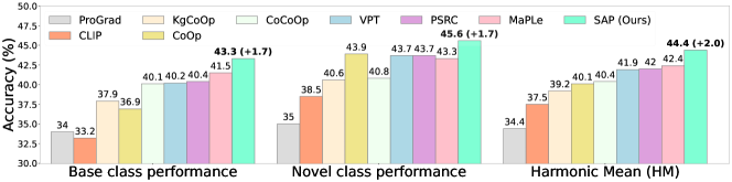
Figure 4: Comparison in the CwC setting. We show average Base, Novel, and HM accuracies over all 11 datasets. During evaluation, descriptions of each class are provided instead of the class name, and visual recognition is conducted based on these descriptions. SAP outperforms baselines by average Base (by $+1.75\%$), Novel (by $+1.76\%$) and HM (by $+2.04$) computed over all datasets.

Classification without Class-names. In this benchmark, we study the ability of a pretrained VLM to classify images without explicit class-names. For all baselines (including ours), for an image $x$ and an unknown class name $y$ with class descriptions $A_{y}$, we find the similarity as $sim(\mathbf{x},y)=\frac{1}{|A_{y}|}\sum\limits_{a\in A_{y}}sim(\mathbf{v}_{pu}^{\mathbf{x}},\mathbf{t}_{p}^{\text{object},a})$, where the class name in the description guided text template is replaced by the word ‘object’. We report average accuracies on 11 datasets in Fig. 4, where we beat MaPLe[15] by +2.04 in HM.

Cross-Dataset generalization. We compare our method with nine baselines and outperform all of them as shown in Tab. 5. SAP outperforms PSRC[16] by +1% and MaPLe[15] by +0.5% on average test accuracy over all datasets, which indicates that our method learns prompts that generalize across datasets.

Dataset	CoOp	CoCoOp	VPT	MaPLe	KgCoOp	ProGrad	PSRC	CLIP-VDT	KAPT	SAP (Ours)
Avg. on 10 Datasets	63.88	65.74	63.42	66.30	65.49	57.36	65.81	53.98	61.50	66.85 (+0.55)

Table 5: Cross-Dataset Generalization benchmark. Models are trained on Imagenet and tested on the entire label space of new datasets without fine-tuning. SAP outperforms all baselines on average.

5.2 Additional Results

Class Activation Maps. We show CAMs for the ResNet-50[10] backbone encoder to visualize image regions that most correlate to a given description.

Figure 5: Class Activation Maps

In addition to Fig. 1, Fig. 5 shows the GradCAM [33] visualizations for novel class “River” w.r.t class description “A photo of a river, is a flowing body of water which has shores” and for class “Spring Crocus” w.r.t description “A photo of a Spring Crocus, has vibrant purple petals which grow in clusters”. SAP effectively localizes the text semantics in image compared to baselines.

Study on Leveraging Class Descriptions for Text Features. In this section we justify our design choice of averaging various class description guided semantic views to generate unified text feature.

Method	Avg HM
SAP	80.94
SAP w/ norm	80.31
SAP w/ agg descriptions	79.17
CLIP-VDT Text + SAP’s Visual	78.63

Table 6: Comparison with other text design alternatives.

Our key contribution is not just integrating descriptions into prompt learning for VLMs, but how descriptions are integrated into both visual and text modalities. We show average HM results across all 11 datasets of other design choices herein, including CLIP-VDT[24]. We consider three alternative ways to incorporate class descriptions and show that our methodology leads to the best results. For our first alternative, we show that normalizing the unified text feature leads to a drop in performance (SAP w/ norm in Tab. 6). We also find that simply appending all class descriptions at once to generate a single semantic view also leads to a drop in performance (SAP w/ agg descriptions in Tab. 6). Finally we show that replacing our text modality construction with that used by CLIP-VDT leads to a significant drop in average HM. These experiments show that how we add class descriptions is important, and that our approach is different from recent approaches that uses external information.

Effect of Removing Learnable Bias. To study the effect of adding a learnable bias to obtain grid features, we conduct an ablation study. Tab. 7 shows that adding a bias is a parameter-efficient way to learn good local image features.

Effect of Removing Class Descriptions. Our method SAP incorporates class descriptions in both image and text modalities, as described in § 4.2 & § 4.3. Here we study the effect of removing description guidance from both modalities. To remove description guidance from images, we simply use the global feature $\mathbf{v}_{pg}$ to compute $L_{ce}$ instead of the unified feature $\mathbf{v}_{pu}$. We denote this by SAP-VG.

Method	Avg. Base	Avg. Novel	Avg. HM
Effect of Removing Learnable Bias
SAP w/o bias	84.55	75.72	79.9
SAP	84.68	77.51	80.94
Effect of Removing Class descriptions
SAP - TG	84.62	74.79	79.41
SAP - VG	84.56	77.04	80.63
SAP	84.68	77.51	80.94
Effect of Unified Image Features
SAP w/ global	84.56	77.04	80.63
SAP w/ global & grid	84.66	76.81	80.55
SAP	84.68	77.51	80.94

Table 7: Ablation Studies. All results are on the B2N generalization benchmark, and are average results over 11 datasets.

Similarly, to remove description guidance from text, we just use the default class name template i.e. ‘a photo of a [y]’. We denote this baseline as SAP-TG. The results shown in Tab. 7 indicate that adding class descriptions to both modalities, as SAP does, is best performing. Furthermore our method to incorporate class descriptions into images is through a fully non-parametric cross-attention, and adds little computational overhead.

Effect of Unified Image Feature. Here we study the goodness of the unified image feature $\mathbf{v}_{pu}$. As described in § 4.3, class descriptions are incorporated into the grid features to generate description guided image views which are averaged into local features and finally fused into unified features. We consider a baseline that uses just the global image feature $\mathbf{v}_{pg}$ instead of the unified feature. We call this SAP w/ global. Then, we consider a baseline that naively combines global and grid features (without constructing semantic-views) by averaging them and denoting it by SAP w/ global & grid. Note that both baselines construct description guided text views. The results presented in Tab. 7 justify our choice of using semantic-views of grid features to generate unified image features.

6 Conclusions

Prompt learning has emerged as a valuable technique for fine-tuning VLMs for downstream tasks. However, existing methods encounter challenges such as overfitting due to limited training data and difficulties handling larger label spaces during evaluation, resulting in bias towards seen classes. Additionally, these methods struggle when class labels are not present in the vocabulary. We study if better text semantics can improve prompt learning, and propose an approach, named SAP, that learns prompts which better generalize to novel classes. Our proposed approach highlights that careful part-level semantic alignment between image and text features is crucial to leverage additional semantic information. We showcase the efficacy of our approach across four benchmarks, demonstrating significant improvements. We hope this work inspires further exploration into leveraging class descriptions in VLMs.

Appendix

In this appendix, we present the following details, which we could not include in the main paper due to space constraints.

• List of notations used in this paper and their descriptions are in § 0.A.

• Overall algorithm of SAP is presented in § 0.B.

• Implementation details are in § 0.C.

• Expanded dataset-wise tables, and additional experiments are presented in § 0.D.

• Examples of class descriptions generated using GPT-3.5 are presented in § 0.E.

• Limitations and Broader Impact in § 0.F.

Appendix 0.A Summary of Notations and Terminology

We denote vectors, matrices, and tensors using small-case bold letters. We use capital-case bold letters to denote batched data. E.g., $\mathbf{x}$ denotes a single image, and $\mathbf{X}$ denotes a batch of images. We use $\cdot$ (dot) to represent various types of multiplication operations – matrix multiplication, matrix-vector or vector-matrix product, and vector dot-product. Detailed descriptions of notations are presented in Tab. A1.

Notation	Description	Dimension
$\mathcal{I}$	Image Encoder
$\mathcal{T}$	Text Encoder
$\mathcal{Y}$	Classification label space
$\theta$	Set of all learnable text and visual prompts
$B$	Batch size
$M$	Number of grid tokens
$N$	Size of the set of descriptions
$n$	Number of the learnable prompt tokens
$d$	Dimension of the multimodal space
$A_{y}$	LLM generated descriptions for class $y$
$A$	Union of all descriptions of the classification label space
$\mathbf{t}^{A}$	Unprompted text features of all descriptions	$\mathbb{R}^{N\times d}$
$\mathbf{t}^{y,j}$	Unprompted description guided text view
	for class $y$ and description $j$	$\mathbb{R}^{d}$
$\mathbf{t}^{y,j}_{p}$	Prompted description guided text view for
	class $y$ and description $j$	$\mathbb{R}^{d}$
$\mathbf{v}_{g}$	Unprompted global image feature	$\mathbb{R}^{d}$
$\mathbf{v}_{pg}$	Prompted global image feature	$\mathbb{R}^{d}$
$\mathbf{v}_{pr}$	Prompted grid image feature	$\mathbb{R}^{M\times d}$
$\mathbf{x}_{att}$	Cross-attention map for an image computed
	using its grid image feature and all descriptions	$\mathbb{R}^{N\times M}$
$\hat{\mathbf{v}}_{pr}$	Prompted description guided views of a single image	$\mathbb{R}^{N\times d}$
$\mathbf{r}_{att}$	Description relevance score for an image	$\mathbb{R}^{N}$
$\mathbf{v}_{pl}$	Prompted local image feature	$\mathbb{R}^{d}$
$l_{s}$	Local score of an image	$\mathbb{R}$
$\mathbf{v}_{pu}$	Prompted unified image feature	$\mathbb{R}^{d}$

Table A1: Notations used in this paper and their descriptions. We denote batched features using bold capital letters. E.g., $\mathbf{V}_{pu}$ are the prompted unified image features for a batch of images.

Appendix 0.B Algorithm

Algorithm 1 outlines the SAP methodology. The algorithm is summarized as follows: In a given dataset, descriptions for each class are acquired by querying the LLM (L1 - L4). Class description features are then derived by passing the descriptions through $\mathcal{T}$ (L5). Unprompted and prompted image features are obtained by processing images through $\mathcal{I}$ (L7-L8). The description-guided image views are obtained via a parameter-free cross-attention between grid features and description features (L9-L10). The local image features are a weighted average of the description-guided views based on the relevance of each description to the image (L11 - L12). Finally, the local and global image features are fused to create the unified image feature (L13 - L14). Unprompted and prompted description-guided text views are obtained by passing the description-guided text templates through $T$ (L15-L16). $L_{ce}$, $L_{steer}^{v}$, and $L_{steer}^{t}$ loss functions are employed to train the prompts.

Algorithm 1 SAP Algorithm

0: Dataset D = $\{\mathbf{x}_{i},y_{i}\}_{i=1}^{B}$; Classification label space: $\mathcal{Y}$; Vision and Language encoders: (${\mathcal{I}}$, ${{\mathcal{T}}}$); LLM: ChatGPT-3.5 model; Hyperparameters: coefficients $\lambda_{1}$,$\lambda_{2}$, scaling parameter $s$, learning rate $\delta$; Learnable Prompts: $\theta=\{\mathcal{P}_{t},\mathcal{P}_{v}\}$

0: Trained parameters $\hat{\theta}$/* Get descriptions for each class by querying LLM */

1: for all y $\in$ $\mathcal{Y}$ do

2:    $A_{y}$ = LLM(Visual features for distinguishing $y$ in a photo?)

3: end for

4: $A=\bigcup\limits_{y\in\mathcal{Y}}$$A_{y}$

5: $\mathbf{t}^{{A}}$ = ${\mathcal{T}}$($A$) /* Get class description features */

6: for all epochs do

6:    /* Get unprompted and prompted image features for every image $\mathbf{x}$ in the batch */

7:    $\mathbf{v}_{g}$, _ = ${\mathcal{I}}$($\mathbf{x}$)

8:    $\mathbf{v}_{pg}$, $\mathbf{v}_{pr}$ = $\mathcal{I}$($\mathbf{x}$; $P_{v}$)/* Get description-guided image views using parameter-free cross-attention */

9:    $\mathbf{x}_{att}$ = $row\_softmax(\mathbf{t}^{A}$ $\cdot$ $\mathbf{v}_{pr}^{\intercal}$)

10:    $\hat{\mathbf{v}}_{pr}$ = $\mathbf{x}_{att}$ $\cdot$ $\mathbf{v}_{pr}$/* Get local image feature using description relevance score and image views */

11:    $\mathbf{r}_{att}=softmax(\mathbf{v}_{pg}\cdot(\textbf{t}^{A})^{\intercal})$

12:    $\mathbf{v}_{pl}$ = $\mathbf{r}_{att}$ $\cdot$$\hat{\mathbf{v}}_{pr}$/* Get unified image feature by fusing global and local feature using local score $l_{s}$ */

13:    $l_{s}$ = $\mathbf{r}_{att}$ $\cdot$ $max(\mathbf{x}_{att},dim=1)$

14:    $\mathbf{v}_{pu}$ = ($1-l_{s}$) $\cdot$ $\mathbf{v}_{pg}$ + $l_{s}$ $\cdot$ $\mathbf{v}_{pl}$/* Get unprompted and prompted description guided text views for every class $y$ */

15:    $\mathbf{t}^{y,A_{y}}$ = ${\mathcal{T}}(y,A_{y})$

16:    $\mathbf{t}^{y,A_{y}}_{p}$ = ${\mathcal{T}}(y,A_{y};P_{t}$)/* Similarity between an image and a class is the aggregate of similarities over pertinent descriptions of a class */

17:    $O_{\theta}(\mathbf{x}_{i},y)=\frac{1}{|A_{y}|}\sum_{a\in A_{y}}sim(\mathbf{v}_{pu}^{\mathbf{x}_{i}}(\theta),\mathbf{t}_{p}^{y,a}(\theta))$

18:    $L_{ce}(\theta)=-\frac{1}{B}\sum\limits_{i=1}^{B}log\frac{exp(s\cdot O_{\theta}(\mathbf{x}_{i},y_{i}))}{\sum\limits_{y\in\mathcal{Y}}exp(s\cdot O_{\theta}(\mathbf{x}_{i},y))}$/* Compute Steering Losses */

19:    $L_{steer}^{v}(\theta)=\frac{1}{B}\sum\limits_{i=1}^{B}\lVert\mathbf{v}_{pg}^{\mathbf{x}_{i}}(\theta)-\mathbf{v}_{g}^{\mathbf{x}_{i}}\rVert_{1}$

20:    $L_{steer}^{t}(\theta)=\frac{1}{|\mathcal{Y}|}\sum\limits_{y\in\mathcal{Y}}\lVert\mathbf{t}_{p}^{y,A_{y}}(\theta)-\mathbf{t}^{y,A_{y}}\rVert_{1}$/* Perform gradient descent on the total loss */

21:    $\small{\mathcal{L}(\theta)=L_{ce}(\theta)+\lambda_{1}L_{steer}^{v}(\theta)+\lambda_{2}L_{steer}^{t}(\theta)}$

22:    $\hat{\theta}$ = $\theta$ - $\delta\nabla$ $\mathcal{L}(\theta)$

23: end for

24: return  $\hat{\theta}$

Appendix 0.C Implementation Details

Training Details. We use the ViT-B/16 [4]-based CLIP model as our backbone. For the GZS and B2N benchmarks, we fine-tune the model on $K=16$ shot training data from the base classes. Prompts are learned in the first three layers for the Cross-dataset benchmark and the first nine layers for the remaining two benchmarks. We introduce a $d$-dimensional bias as the sole additional parameter compared to  [16]. The text prompts in the initial layer are initialized with the word embeddings of ‘a photo of a’, and the rest are randomly initialized from a normal distribution, similar to [16]. Our models are trained on a single Tesla V100 GPU with Nvidia driver version 470.199.02. We train for $20$ epochs, with a batch size of 4 images, $\lambda_{1}=10$ and $\lambda_{2}=25$. The hyperparameter setup is common across all datasets. We use the SGD optimizer with a momentum of $0.9$, a learning rate of $0.0025$, and weight decay $5e-4$. A cosine learning rate scheduler is applied with a warmup epoch of $1$. Image pre-processing involves random crops, random horizontal and vertical flips, and normalization using mean values of $[0.48,0.46,0.41]$ and standard deviation values of $[0.27,0.26,0.27]$. All baselines utilize publicly available codes and models. All results are averages over three seeds. We use PyTorch 1.12, CUDA 11.3, and build on the Dassl code repository: https://github.com/KaiyangZhou/Dassl.pytorch. We will open-source our code on acceptance.

Appendix 0.D Expanded Tables and Additional Results

Using Random Text in place of Class Descriptions. To study the usefulness of valid descriptions, we replace the descriptions for each class by randomly generated texting in Tab. A2. Examples of random descriptions are “Raindrops pattered softly against the roof”, “A solitary figure walked down the empty street”. We observe that descriptions matter for unusual datasets having texture-based images, satellite images, aircraft images and action recognition images. The average HM using random text across 11 datasets on B2N benchmark is 78.27, while SAP reports an average HM of 80.94. A drop of 2.67 is noted.

	UCF101	EuroSAT	DTD	OxfordPets	StanfordCars	Flowers102	Food101	FGVCAircraft	SUN397	Caltech101	ImageNet	Average
Base	86.27	95.83	83.1	95.07	78.2	97.5	90.13	41.37	81.87	98.07	76.7	84.01
Novel	76.37	69.23	54.1	95.33	72.33	75.53	89.9	34.8	76.63	94.1	67.7	73.27
HM	81.02	80.39	65.54	95.2	75.15	85.12	90.01	37.8	79.16	96.04	72.17	78.27

Table A2: B2N benchmark results using random text in place of class descriptions. The results show that using irrelevant descriptions hurts model performance.

Few-shot Setting. Our main objective is to train prompts that can generalize effectively to novel classes and datasets. As such, we present results primarily on settings that test generalizability, such as the GZS benchmark, Base-to-Novel benchmark, and the Classification without class names benchmark. For completeness, we present results in a few-shot classification setting, where limited training samples are provided for all classes. Note that there are no novel classes in this setting. We showcase outcomes for $K=1,2,4,8,\text{and }16$ shots. As shown in Fig. A1, on average, across 11 datasets, we perform competitively against the best baseline PSRC.

	Source	Target
	ImageNet	-V2	-A	-S	-R	Avg
MaPLe	77.10	71.00	53.70	50.00	77.70	63.10
PSRC	76.30	71.00	54.10	50.00	77.80	63.22
SAP	76.40	71.10	55.70	49.80	77.50	63.52

Table A3: DG benchmark. SAP outperforms baselines on avg.

Domain Generalization. We show results on Domain Generalization in Tab. A3. We train on $K=16$ shot training data from base classes of source dataset ImageNet and evaluation on ImageNetV2, ImageNet-A, ImageNet-Setch, and ImageNet-R target datasets. SAP outperforms two strong baselines PSRC and MaPLe.

ResNet-50 Backbone as Image Encoder. Herewe show the GZS and B2N performance of SAP using the ResNet-50 CLIP model as a backbone. We compare against five baselines which also use the ResNet-50 backbone and present our results in Tab. A4. For all methods including ours, we train the models without tuning any hyperparameters such as prompt-depth, regularization weight, learning rate etc. and use the same values as those of ViT-B/16 CLIP backbone. We observe that PSRC performs particularly poorly with a ResNet backbone. Although we use similar hyperparameters as PSRC, SAP shows good results, indicating that class descriptions help greatly in this setting. We show a gain of +0.98 on average gHM for GZS, and +2.32 on average HM in the B2N setting.

Dataset		CLIP	CoOp	KgCoOp	ProGrad	PSRC	SAP (Ours)
Generalized Zero-Shot Learning Benchmark
Average on 11 datasets	gBase	57.01	68.65	69.25	69.89	47.41	71.52 (+1.63)
	gNovel	60.73	50.35	59.08	52.26	29.16	59.13 (-1.60)
	gHM	58.81	58.1	63.76	59.81	36.12	64.74 (+0.98)
Base-to-Novel Generalization Benchmark
Average on 11 datasets	Base	65.27	77.24	75.51	77.98	55.13	78.49 (+0.51)
	Novel	68.14	57.40	67.53	63.41	38.72	69.32 (+1.79)
	HM	66.68	65.86	71.30	69.94	45.49	73.62 (+2.32)

Table A4: Results on GZS and B2N settings using a ResNet-50 backbone. On average, SAP outperforms all the baselines.

Depth	1	3	5	7	9	11
HM	76.84	79.35	79.25	80.85	81.76	80.68

Table A5: Prompt depth analysis

Prompt Depth. Tab. A5 shows the average HM for the B2N benchmark across nine datasets, excluding SUN397 and ImageNet. As seen from the table, adding prompts till depth 9 for image and text encoders is ideal for SAP performance and is used for B2N, GZS and CwC benchmarks.

Additional Class Activation Maps (CAMs). We show additional CAMs for the ResNet-50[10] backbone encoder to visualize image regions that most correlate to a given description. Fig. A2 shows the GradCAM [33] visualizations for base classes “Floor gymnastics” w.r.t class description “A photo of a floor gymnastics, which has a person performing flips or somersaults”, class “Hammering” w.r.t description “A photo of a hammering, which has a person holding a hammer”, class “Cape Flower” w.r.t class description “A photo of a cape flower, which has vibrant and colorful petals”, class “Highway” w.r.t class description “A photo of a highway, which is a long and straight path”. SAP effectively localizes the text semantics in the image compared to baselines.

Expanded Dataset-wise Tables. We present the elaborate tables dataset-wise for the Generalized Zero-Shot setting in Tab. A6 and Base-to-Novel generalization setting in Tab. A7. SAP outperforms the best-performing baseline, PSRC, in 7 of the 11 considered datasets. We perform very well in challenging datasets such as EuroSAT, DTD, and UCF-101. We present dataset-wise results for the Classification without class name benchmark in Tab. A8. Tab. A10 has the dataset-wise results for the Cross-Dataset generalizatin benchmark. In Tab. A4 we show average results on the GZS benchmark and the Base-to-Novel benchmark for the ResNet-50 backbone Image Encoder. We also present detailed, dataset-wise results for the same in Tab. A9.

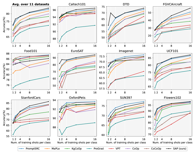
Figure A1: Performance of SAP in the few-shot setting. Our method achieves competitive performance compared to all baselines on average across 11 datasets.

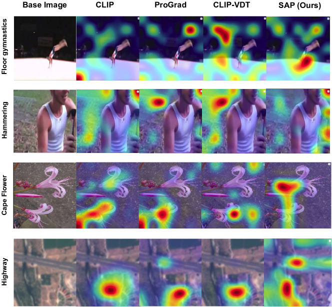
Figure A2: Class activation maps

Dataset		CLIP	CoOp	VPT	CoCoOp	MaPLe	KgCoOp	ProGrad	PSRC	CLIP-VDT	SAP
		(ICML ’21)	(IJCV ’22)	(ECCV ’22)	(CVPR ’22)	(CVPR ’23)	(CVPR ’23)	(ICCV ’23)	(ICCV ’23)	(ICCVW ’23)	(Ours)
Average	gBase	60.81	75.19	73.48	73.13	75.47	76.86	70.15	78.81	63.75	79.47 (+0.66)
on 11	gNovel	63.21	60.39	66.62	65.23	67.09	62.12	55.07	68.13	63.89	69.75 (+1.62)
datasets	gHM	61.99	66.99	69.89	68.96	71.04	68.71	61.70	73.08	63.82	74.29 (+1.21)
UCF101	gBase	62.70	80.26	75.76	76.56	76.90	78.96	74.63	82.67	66.19	82.23
	gNovel	64.40	84.76	67.73	64.76	70.40	62.33	51.36	71.40	67.00	76.40
	gHM	63.53	82.45	71.52	70.17	73.51	69.67	60.85	76.62	66.59	79.21
EuroSAT	gBase	51.40	69.26	88.22	70.86	84.06	82.02	76.26	86.60	55.09	94.37
	gNovel	38.90	36.26	53.36	41.03	43.90	31.26	23.43	54.16	50.79	58.53
	gHM	44.28	47.60	66.50	51.97	57.68	45.28	35.85	66.65	52.85	72.25
DTD	gBase	42.70	65.36	58.92	60.29	63.00	66.42	57.19	68.73	55.79	66.47
	gNovel	45.79	34.30	44.26	46.09	47.49	39.73	33.36	47.53	51.00	54.27
	gHM	44.19	44.99	50.55	52.25	54.16	49.72	42.14	56.20	53.28	59.75
Oxford Pets	gBase	84.80	89.56	89.06	91.12	91.69	91.99	88.36	93.00	83.80	91.97
	gNovel	90.19	90.46	93.23	92.50	93.93	92.69	87.76	91.00	90.40	92.30
	gHM	87.41	90.01	91.10	91.81	92.80	92.34	88.06	91.99	86.97	92.13
Stanford Cars	gBase	56.00	74.43	65.13	67.29	69.33	72.56	64.46	74.77	59.50	76.40
	gNovel	64.19	57.16	70.56	68.82	69.86	66.56	55.66	71.23	61.59	69.33
	gHM	59.81	64.67	67.74	68.05	69.61	69.43	59.74	72.96	60.52	72.69
Flowers102	gBase	62.09	93.40	83.12	87.36	91.19	92.80	84.86	95.00	69.90	95.69
	gNovel	69.80	56.92	65.56	65.53	68.29	65.76	62.39	71.00	77.00	71.13
	gHM	65.71	70.74	73.31	74.89	78.10	76.97	71.92	81.27	73.20	81.60
Food101	gBase	79.90	83.59	85.96	86.15	86.76	85.76	78.46	87.07	75.90	86.43
	gNovel	80.90	76.82	84.99	86.50	87.20	83.72	76.23	85.90	77.69	86.09
	gHM	80.39	80.07	85.49	86.33	86.98	84.73	77.33	86.48	76.78	86.26
FGVC Aircraft	gBase	14.50	29.92	25.12	25.90	25.90	32.69	23.93	34.90	16.10	35.00
	gNovel	23.79	22.83	28.03	26.36	28.53	22.06	15.63	28.40	18.60	30.23
	gHM	18.01	25.90	26.50	26.13	27.15	26.35	18.93	31.32	17.59	32.44
SUN397	gBase	60.50	72.56	69.40	71.19	72.76	73.36	67.69	75.63	63.09	75.40
	gNovel	63.70	56.52	67.50	67.26	68.93	61.75	57.00	68.70	66.00	69.80
	gHM	62.05	63.55	68.44	69.17	70.79	67.06	61.89	72.00	64.51	72.30
Caltech101	gBase	91.40	95.92	95.66	95.09	95.83	95.89	91.53	96.20	93.59	96.30
	gNovel	91.69	85.09	92.26	90.93	92.03	92.06	85.26	91.73	86.19	92.82
	gHM	91.54	90.19	93.94	92.97	93.89	93.94	88.29	93.91	89.73	94.53
Imagenet	gBase	63.00	72.80	71.9	72.59	72.80	73.00	64.19	72.30	61.79	73.97
	gNovel	62.00	63.20	65.40	67.80	67.40	65.40	57.70	68.40	56.59	66.66
	gHM	62.49	67.66	68.50	70.11	70.00	68.99	60.77	70.30	59.07	70.13

Table A6: Accuracy comparison on the GZS benchmark. gNovel & gBase indicate the accuracy of the novel classes and base classes respectively under the joint classification label space. gHM is the harmonic mean of gBase and gNovel. The best numbers are in bold, and the second best are underlined. As reported in the first row, SAP outperforms all baselines on average gBase (by $+0.66\%$), gNovel (by $+1.62\%$), and gHM (by $1.21\%$) computed across all datasets. We indicate the margin of improvement over the corresponding best-performing baseline for each metric in green.

Dataset		CLIP	CoOp	VPT	CoCoOp	ProDA	MaPLe	KgCoOp	ProGrad	PSRC	L.Prompt	CLIP-VDT	KAPT	SAP
Average	Base	69.34	82.69	80.81	80.47	81.56	82.28	80.73	82.48	84.26	84.47	82.48	81.10	84.68 (+0.21)
on 11	Novel	74.22	63.22	70.36	71.69	72.30	75.14	73.60	70.75	76.10	74.24	74.50	72.24	77.51 (+1.41)
datasets	HM	71.70	71.66	70.36	75.83	76.65	78.55	77.00	76.16	79.97	79.03	78.28	76.41	80.94 (+0.97)
UCF101	Base	70.53	84.69	82.67	82.33	85.23	83.00	82.89	84.33	87.10	86.19	84.10	80.83	86.60
	Novel	77.50	56.05	74.54	77.64	78.04	80.77	76.67	76.94	78.80	73.07	76.40	67.10	83.90
	HM	73.85	67.46	78.39	77.64	78.04	80.77	79.65	79.35	82.74	79.09	80.07	73.33	85.23
EuroSAT	Base	56.48	92.19	93.01	87.49	83.90	94.07	85.64	90.11	92.90	93.67	88.50	84.80	96.10
	Novel	64.05	54.74	54.89	60.04	66.00	73.23	64.34	60.89	73.90	69.44	70.50	67.57	81.13
	HM	60.03	68.69	69.04	71.21	73.88	82.35	73.48	72.67	82.32	79.75	78.48	75.21	87.98
DTD	Base	53.24	79.44	79.15	77.01	80.67	80.36	77.55	77.35	83.37	82.87	81.80	75.97	84.27
	Novel	59.90	41.18	50.76	56.00	56.48	59.18	54.99	52.35	62.97	60.14	62.30	58.30	67.03
	HM	56.37	54.24	61.85	64.85	66.44	68.16	64.35	62.45	71.75	69.70	70.73	65.97	74.67
Oxford Pets	Base	91.17	93.67	94.81	95.20	95.43	95.43	94.65	95.07	95.33	96.07	94.40	93.13	95.27
	Novel	97.26	95.29	96.00	97.69	97.83	97.76	97.76	97.63	97.30	96.31	97.70	96.53	96.90
	HM	94.12	94.47	95.40	96.43	96.62	96.58	96.18	96.33	96.30	96.18	95.68	94.80	96.08
Stanford Cars	Base	63.37	78.12	72.46	70.49	74.70	72.94	71.76	77.68	78.27	78.36	76.80	69.47	79.70
	Novel	74.89	60.40	73.38	73.59	71.20	74.00	75.04	68.63	74.97	72.39	72.90	66.20	73.47
	HM	68.65	68.13	72.92	72.01	72.91	73.47	73.36	72.88	76.58	75.26	74.80	67.79	76.46
Flowers102	Base	72.08	97.60	95.39	94.87	97.70	95.92	95.00	95.54	98.07	99.05	97.40	95.00	97.83
	Novel	77.80	59.67	73.87	71.75	68.68	72.46	74.73	71.87	76.50	76.52	75.30	71.20	76.50
	HM	74.83	74.06	83.26	81.71	80.66	82.56	83.65	82.03	85.95	86.34	84.94	81.40	86.86
Food101	Base	90.10	88.33	89.88	90.70	90.30	90.71	90.50	90.37	90.67	90.82	90.40	86.13	90.40
	Novel	91.22	82.26	87.76	91.29	88.57	92.05	91.70	89.59	91.53	91.41	91.20	87.06	91.43
	HM	90.66	85.19	88.81	90.99	89.43	91.38	91.09	89.98	91.10	91.11	90.80	86.59	90.91
FGVC Aircraft	Base	27.19	40.44	33.10	33.41	36.90	37.44	36.21	40.54	42.73	45.98	37.80	29.67	42.93
	Novel	36.29	22.30	30.49	23.71	34.13	35.61	33.55	27.57	37.87	34.67	33.00	28.73	38.87
	HM	31.09	28.75	31.74	27.74	35.46	36.50	34.83	32.82	40.15	39.53	35.24	29.19	40.80
SUN397	Base	69.36	80.60	79.66	79.74	78.67	80.82	80.29	81.26	82.67	81.20	81.40	79.40	82.57
	Novel	75.35	65.89	72.68	76.86	76.93	78.70	76.53	74.17	78.47	78.12	76.80	74.33	79.20
	HM	72.23	72.51	79.63	78.27	77.79	79.75	78.36	77.55	80.52	79.63	79.03	76.78	80.85
Caltech101	Base	96.84	98.00	97.86	97.96	98.27	97.74	97.72	98.02	98.10	98.19	98.30	97.10	98.23
	Novel	94.00	89.91	93.76	93.81	93.23	94.36	94.39	93.89	94.03	93.78	95.90	93.53	94.37
	HM	95.40	93.73	95.77	95.84	95.68	96.02	96.03	95.91	96.02	95.93	97.09	95.28	96.26
ImageNet	Base	72.43	76.47	70.93	75.98	75.40	76.66	75.83	77.02	77.60	76.74	76.40	71.10	77.60
	Novel	68.14	67.88	65.90	70.43	70.23	70.54	69.96	66.66	70.73	70.83	68.30	65.20	69.83
	HM	70.22	71.92	73.66	73.10	72.72	73.47	72.78	71.46	74.01	73.66	72.12	68.02	73.51

Table A7: Accuracy comparison on Base-to-Novel Generalization benchmark. The best numbers are in bold, and the second best are underlined. SAP outperforms all baselines on average Base (by $+0.21\%$), Novel (by $+1.41\%$) and HM (by $+0.97\%$) computed over all datasets. We indicate the margin of improvement over the corresponding best-performing baseline for each metric in green.

Dataset		CLIP	CoOp	VPT	CoCoOp	MaPLe	KgCoOp	ProGrad	PSRC	SAP
Average	Base	33.28	36.97	40.28	40.12	41.56	37.95	34.00	40.40	43.31 (+1.75)
on 11	Novel	38.55	43.90	43.72	40.80	43.30	40.69	35.01	43.78	45.66 (+1.76)
datasets	HM	35.72	40.14	41.93	40.46	42.41	39.27	34.50	42.02	44.46 (+2.04)
UCF101	Base	56.60	61.20	61.20	61.70	64.20	62.00	59.70	63.10	64.70
	Novel	62.20	66.80	63.20	70.70	70.40	68.80	63.50	69.40	69.10
	HM	59.27	63.88	62.18	65.89	67.16	65.22	61.54	66.10	66.83
EuroSAT	Base	39.90	47.10	76.50	62.90	84.30	59.70	47.60	71.4	88.70
	Novel	71.10	78.70	83.20	49.00	58.30	57.60	45.80	82.10	80.90
	HM	51.12	58.93	79.71	55.09	68.93	58.63	46.68	76.38	84.62
DTD	Base	40.20	40.90	47.20	44.20	44.90	41.90	39.20	42.70	52.40
	Novel	42.40	44.10	44.30	47.10	42.90	44.40	40.20	44.00	49.00
	HM	41.27	42.44	45.70	45.60	43.88	43.11	39.69	43.34	50.64
Oxford Pets	Base	24.50	32.00	22.30	34.20	32.80	25.40	23.10	27.40	23.60
	Novel	35.20	40.80	40.70	44.10	46.40	39.70	36.00	41.60	44.10
	HM	28.89	35.87	28.81	38.52	38.43	30.98	28.14	33.04	30.75
Stanford Cars	Base	13.50	15.60	17.60	16.30	10.30	12.50	10.00	21.00	22.50
	Novel	15.90	20.70	18.90	11.70	25.80	15.30	8.50	20.40	23.40
	HM	14.60	17.79	18.23	13.62	14.72	13.76	9.19	20.70	22.94
Flowers102	Base	7.40	14.10	12.40	17.70	18.30	12.00	16.40	18.80	19.60
	Novel	9.30	20.40	18.40	17.60	23.20	12.30	13.80	19.30	26.00
	HM	8.24	16.67	14.82	17.65	20.46	12.15	14.99	19.05	22.35
Food101	Base	35.10	42.70	44.00	43.40	35.50	47.10	42.10	41.20	42.20
	Novel	33.80	45.40	44.80	44.40	38.90	44.60	41.80	40.50	44.20
	HM	34.44	44.01	44.40	43.89	37.12	45.82	41.95	40.85	43.18
FGVC Aircraft	Base	6.10	9.50	8.00	7.00	13.40	6.80	5.20	8.30	9.40
	Novel	7.90	15.80	12.80	8.30	15.50	10.70	8.20	12.30	12.30
	HM	6.88	11.87	9.85	7.59	14.37	8.32	6.36	9.91	10.66
SUN397	Base	46.60	49.20	50.50	51.30	50.20	50.10	40.10	50.00	51.40
	Novel	48.30	50.00	51.40	52.50	52.20	53.20	42.90	51.40	51.40
	HM	47.43	49.60	50.95	51.89	51.18	51.60	41.45	50.69	51.40
Caltech101	Base	77.80	76.00	83.00	83.00	82.30	80.80	72.30	81.10	81.70
	Novel	74.80	74.30	75.90	75.80	75.50	76.20	63.20	75.10	75.20
	HM	76.27	75.14	79.29	79.24	78.75	78.43	67.44	77.98	78.32
ImageNet	Base	18.40	18.40	20.40	19.70	21.00	19.20	18.30	19.4	20.30
	Novel	23.20	26.00	27.40	27.60	27.30	24.80	21.30	25.50	26.70
	HM	20.52	21.55	23.39	22.99	23.74	21.64	19.69	22.04	23.06

Table A8: Accuracy comparison in the classification without class names setting. We show average Base, Novel, and HM accuracies over all 11 datasets. During evaluation, descriptions of each class are provided instead of the class name, and visual recognition is conducted based on these descriptions. SAP outperforms baselines by average Base (by $+1.75\%$), Novel (by $+1.76\%$) and HM (by $+2.04\%$) computed over all datasets.

	GZS Benchmark							Base-to-Novel Benchmark
Dataset		CLIP	CoOp	KgCoOp	Pro-	PSRC	SAP		CLIP	CoOp	KgCoOp	Pro-	PSRC	SAP
					Grad							Grad
Average	gBase	57.01	68.65	69.25	69.89	47.41	71.52 (+1.63)	Base	65.27	77.24	75.51	77.98	55.13	78.49 (+0.51)
on 11	gNovel	60.73	50.35	59.08	52.26	29.16	59.13 (-1.60)	Novel	68.14	57.40	67.53	63.41	38.72	69.32 (+1.79)
datasets	gHM	58.81	58.10	63.76	59.81	36.12	64.74 (+0.98)	HM	66.68	65.86	71.30	69.94	45.49	73.62 (+2.32)
UCF101	gBase	61.20	73.20	71.05	72.75	51.55	74.73	Base	68.40	79.78	77.16	81.04	59.95	80.70
	gNovel	61.79	45.10	56.95	48.05	30.25	63.80	Novel	61.50	48.31	70.13	60.07	38.85	72.67
	gHM	61.49	55.81	63.22	57.87	38.13	68.33	HM	64.77	60.18	73.48	69.00	47.15	76.47
EuroSAT	gBase	32.79	62.70	71.25	73.60	61.15	72.77	Base	55.80	90.25	84.28	88.44	70.35	91.33
	gNovel	46.50	23.45	33.95	19.40	09.00	32.32	Novel	66.90	31.30	53.53	49.49	33.90	67.00
	gHM	38.46	34.13	45.99	30.71	15.69	44.76	HM	60.85	46.48	65.47	63.47	45.75	77.30
DTD	gBase	43.50	60.60	64.80	62.30	42.60	62.73	Base	53.70	75.12	74.73	73.80	51.35	75.97
	gNovel	41.29	27.05	40.45	27.05	18.30	44.27	Novel	55.60	37.08	48.39	46.38	29.85	57.90
	gHM	42.37	37.40	49.81	37.72	25.60	51.91	HM	54.63	49.65	58.74	56.96	37.75	65.72
Oxford Pets	gBase	85.90	84.70	85.75	85.95	67.65	87.00	Base	91.20	90.15	92.57	92.36	77.60	91.90
	gNovel	85.59	85.25	90.45	87.10	65.65	89.27	Novel	93.90	90.70	94.61	94.48	79.40	94.57
	gHM	85.74	84.97	88.04	86.52	66.63	88.12	HM	92.53	90.42	93.58	93.41	78.49	93.22
Stanford Cars	gBase	48.29	64.70	62.25	64.30	17.35	68.20	Base	55.50	68.89	63.28	71.79	26.35	71.43
	gNovel	64.09	48.05	59.20	53.45	21.65	57.60	Novel	66.50	57.13	66.92	59.36	25.50	64.77
	gHM	55.08	55.15	60.69	58.38	19.26	62.45	HM	60.50	62.46	65.05	64.99	25.92	67.94
Flowers102	gBase	62.59	89.40	85.70	88.80	65.00	92.52	Base	69.70	95.22	91.45	94.71	73.75	96.40
	gNovel	68.30	50.70	63.85	52.75	10.85	61.62	Novel	73.90	59.53	71.75	68.86	19.75	70.30
	gHM	65.32	64.70	73.18	66.18	18.60	73.97	HM	71.74	73.26	80.41	79.74	31.16	81.31
Food101	gBase	75.80	73.80	78.30	76.30	32.65	77.97	Base	83.10	81.70	83.90	83.77	37.85	83.57
	gNovel	78.90	68.50	78.25	72.90	17.60	76.60	Novel	84.50	78.13	85.23	83.74	27.15	84.13
	gHM	77.32	71.05	78.27	74.56	22.87	77.28	HM	83.79	79.88	84.56	83.75	31.62	83.85
FGVC Aircraft	gBase	12.69	24.15	20.20	21.60	8.65	23.17	Base	18.80	28.39	24.91	30.17	14.20	28.97
	gNovel	22.10	14.75	18.20	14.25	6.95	17.45	Novel	26.00	20.02	25.69	19.70	9.05	25.33
	gHM	16.12	18.31	19.15	17.17	7.71	19.91	HM	21.82	23.48	25.29	23.84	11.05	27.03
SUN397	gBase	56.70	66.65	67.05	67.15	54.25	70.40	Base	66.40	76.33	75.33	76.90	63.25	78.20
	gNovel	60.50	53.30	61.80	56.50	45.85	62.20	Novel	70.10	62.89	72.25	68.09	57.50	73.27
	gHM	58.54	59.23	64.32	61.37	49.70	66.05	HM	70.10	68.96	73.76	72.23	60.24	75.65
Caltech101	gBase	88.59	91.35	91.65	91.50	79.35	92.13	Base	91.00	95.20	95.35	95.72	84.80	95.67
	gNovel	81.69	82.15	88.05	86.30	58.65	87.50	Novel	90.60	87.55	91.92	89.92	65.65	91.13
	gHM	85.00	86.51	89.81	88.82	67.45	89.76	HM	90.80	91.21	93.60	92.73	74.01	93.34
ImageNet	gBase	59.09	63.90	63.75	64.55	41.40	65.05	Base	64.40	68.5	67.67	69.13	47.00	69.20
	gNovel	57.29	55.60	58.75	57.15	36.05	57.85	Novel	60.10	58.76	62.45	57.39	39.35	61.40
	gHM	58.18	59.46	61.15	60.63	38.54	61.24	HM	62.18	63.29	64.96	62.72	42.84	65.07

Table A9: GZS benchmark and Base-to-Novel Generalization benchmark using ResNet backbone. Metrics for the GZS benchmark, such as gBase, gNovel, and gHM, are employed in the left section of the table. Conversely, metrics like Base, Novel, and HM are utilized to assess the Base-to-Novel benchmark in the right section. On average, our method outperforms all the baselines. We regret the mistake in Tab A4 of the main paper, where we incorrectly stated our method outperformed CLIP in the GZS benchmark. This error will be rectified in the revised version.

	Source	Target
	ImageNet	Caltech101	OxfordPets	StanfordCars	Flowers102	Food101	Aircraft	SUN397	DTD	EuroSAT	UCF101	Average
CoOp	71.51	93.70	89.14	64.51	68.71	85.30	18.47	64.15	41.92	46.39	66.55	63.88
CoCoOp	71.02	94.43	90.14	65.32	71.88	86.06	22.94	67.36	45.73	45.37	68.21	65.74
VPT	70.60	91.80	90.40	63.70	67.30	83.10	22.70	66.10	46.10	37.10	65.90	63.42
MaPLe	70.72	93.53	90.49	65.57	72.23	86.20	24.74	67.01	46.49	48.06	68.69	66.30
KgCoOp	69.94	94.08	90.13	65.63	71.21	86.48	23.85	67.47	45.80	41.98	68.33	65.49
ProGrad	62.17	88.30	86.43	55.61	62.69	76.76	15.76	60.16	39.48	28.47	58.70	57.36
PSRC	71.27	93.60	90.25	65.70	70.25	86.15	23.90	67.10	46.87	45.50	68.75	65.81
CLIP-VDT	68.10	85.40	83.50	50.30	56.00	72.50	14.60	56.30	42.70	24.70	53.80	53.98
KAPT	N/A	88.90	89.40	58.15	68.00	79.95	17.95	N/A	44.80	41.35	65.05	61.50
SAP (Ours)	71.40	94.53	90.14	64.58	71.31	86.23	24.47	68.09	48.61	49.10	71.52	66.85

Table A10: Cross-Dataset Generalization benchmark. Models are trained on Imagenet and tested on the entire label space of new datasets without fine-tuning. SAP outperforms all baselines on average. N/A: not available in [14].

Appendix 0.E Generation of Class Descriptions

Tab. A11 shows class names sampled from different datasets and their respective descriptions retrieved using GPT-3.5 [8]. We use the query – ‘‘What are useful visual features for distinguishing a [classname] in a photo? Answer concisely.’’ Class descriptions differ from well-curated attributes found in datasets with annotated attributes such as AwA [18] and CUB [36] in three ways: (i) Our class descriptions may be noisy since no manual curation is used; (ii) They may not necessarily contain class-discriminative information, especially for similar classes; and (iii) Descriptions of a class are generated independently, and may not contain comparative traits w.r.t. other classes. These choices are primarily to keep our approach low-cost while integrating these finer details into fine-tuning of VLMs. It’s important to note that our description generation occurs at the class level, not the image level, making it cost-efficient.

Appendix 0.F Limitations and Broader Impact

A key dependency of our framework is the need for an LLM to provide descriptions at a class level. We however believe that this has become increasingly feasible in recent times, especially since we require at a class level and not at the image level. Our work deals with learning prompts for generalizable image classification by leveraging cheaply available semantic knowledge in the form of class descriptions. We believe that our work can serve as a stepping stone for incorporating semantic information to solve multi-modal tasks like captioning and VQA. To the best of our knowledge, there are no direct detrimental effects of our work.

Class	Descriptions	Class	Descriptions
(Dataset)		(Dataset)
Breast stroke	1. Arms moving in a circular motion	Diving	1. Person in mid-air or jumping
(UCF101)	2. Kicking legs in a frog-like motion	(UCF101)	2. Person wearing diving gear
	3. Head above water during stroke		3. water splashing or ripples
	4. Positioned horizontally in the water		4. Person wearing gogglesr
	5. Pushing water forward and outwards		5. Person wearing swim cap
Highway or road	1. Long and straight path	Permanent cropland	1. Uniform vegetation or crops
(EuroSAT)	2. Multiple lanes for traffic	(EuroSAT)	2. Irrigation systems or canals
	3. Traffic signs		3. Organized rows or patterns
	4. Smooth and paved surface		4. Fences or boundaries
	5. Guardrails or barriers		5. Distinct crop types or varieties
Striped	1. Alternating bands or lines	Wrinkled	1. Irregular and uneven surface
(DTD)	2. Regular pattern of stripes	(DTD)	2. Creases or folds
	3. Varying widths of stripes		3. Shadows indicating unevenness
	4. Contrasting colors between stripes		4. Lack of smoothness
	5. Horizontal, vertical, diagonal stripes		5. Distorted or crumpled appearance
Maine coon	1. Large domestic cat	Chihuahua	1. Small breed of dog
(Oxford Pets)	2. Long, bushy tail	(Oxford Pets)	2. Rounded apple-shaped head
	3. Tufted ears with lynx-like tips		3. Erect, pointy ears
	4. Rectangular body shape		4. Short snout
	5. Tufted paws		5. Short legs and long tail
2008 chrysler pt	1. Convertible top	2012 ferrari ff coupe	1. Sleek and sporty design
cruiser convertible	2. Chrome grille	(Stanford Cars)	2. Large and stylish alloy wheels
(Stanford Cars)	3. PT cruiser badge		3. Low and wide stance
	4. Alloy wheels		4. Ferrari logo on the front and rear
	5. Boxy shape		5. Dual exhaust pipes
Watercress	1. Small, round-shaped leaves	Trumpet creeper	1. Bright orange or red flowers
(Flowers102)	2. Vibrant green color	(Flowers102)	2. Trumpet-shaped blossoms
	3. Thin, delicate stems		3. Long, tubular petals
	4. Water or moist environments		4. Green leaves with serrated edges
	5. Clusters of small white flowers		5. Hummingbirds and bees
Hot dog	1. Cylindrical-shaped food	Sushi	1. Bite-sized and compact
(Food101)	2. Bun or bread	(Food101)	2. Rice as a base
	3. Sausage or frankfurter		3. Raw or cooked fish
	4. Visible grill marks		4. Seaweed wrapping (nori)
	5. Toppings like onions or relish		5. Served with soy sauce
737-200	1. Two engines on the wings	Industrial area	1. Factories or warehouses
(FGVC Aircraft)	2. Low wing configuration	(SUN397)	2. Smokestacks or chimneys
	3. Narrow body		3. Cranes or heavy machinery
	4. Distinctive short fuselage		4. Conveyor belts or assembly lines
	5. Swept-back wings		5. Trucks or shipping containers
Gramophone	1. Phonograph Cylinder or Disc	Buckle	1. Metal or plastic object
(Caltech101)	2. Horn Speaker	(Imagenet)	2. Rectangular or circular shape
	3. Hand-Cranked Operation		3. Fastening or securing
	4. Nostalgic and Vintage Appeal		4. Opened and closed
	5. Vinyl or Shellac Records		5. Found on belts or straps

Table A11: Sample classes from various datasets and the corresponding descriptions provided by GPT-3.5.

References

- [1] Bossard, L., Guillaumin, M., Gool, L.V.: Food-101 - mining discriminative components with random forests. In: European Conference on Computer Vision (2014), https://api.semanticscholar.org/CorpusID:12726540
- [2] Cimpoi, M., Maji, S., Kokkinos, I., Mohamed, S., Vedaldi, A.: Describing textures in the wild. 2014 IEEE Conference on Computer Vision and Pattern Recognition pp. 3606–3613 (2013), https://api.semanticscholar.org/CorpusID:4309276
- [3] Deng, J., Dong, W., Socher, R., Li, L.J., Li, K., Fei-Fei, L.: Imagenet: A large-scale hierarchical image database. 2009 IEEE Conference on Computer Vision and Pattern Recognition pp. 248–255 (2009), https://api.semanticscholar.org/CorpusID:57246310
- [4] Dosovitskiy, A., Beyer, L., Kolesnikov, A., Weissenborn, D., Zhai, X., Unterthiner, T., Dehghani, M., Minderer, M., Heigold, G., Gelly, S., Uszkoreit, J., Houlsby, N.: An image is worth 16x16 words: Transformers for image recognition at scale. In: International Conference on Learning Representations (2021), https://openreview.net/forum?id=YicbFdNTTy
- [5] Fahes, M., Vu, T.H., Bursuc, A., Pérez, P., de Charette, R.: Pøda: Prompt-driven zero-shot domain adaptation. In: ICCV (2023)
- [6] Fei-Fei, L., Fergus, R., Perona, P.: Learning generative visual models from few training examples: An incremental bayesian approach tested on 101 object categories. 2004 Conference on Computer Vision and Pattern Recognition Workshop pp. 178–178 (2004), https://api.semanticscholar.org/CorpusID:2156851
- [7] Feng, C., Zhong, Y., Jie, Z., Chu, X., Ren, H., Wei, X., Xie, W., Ma, L.: Promptdet: Towards open-vocabulary detection using uncurated images. In: Proceedings of the European Conference on Computer Vision (2022)
- [8] Hagendorff, T., Fabi, S., Kosinski, M.: Machine intuition: Uncovering human-like intuitive decision-making in gpt-3.5 (12 2022). https://doi.org/10.48550/arXiv.2212.05206
- [9] He, K., Zhang, X., Ren, S., Sun, J.: Deep residual learning for image recognition. 2016 IEEE Conference on Computer Vision and Pattern Recognition (CVPR) pp. 770–778 (2015), https://api.semanticscholar.org/CorpusID:206594692
- [10] He, K., Zhang, X., Ren, S., Sun, J.: Deep residual learning for image recognition. 2016 IEEE Conference on Computer Vision and Pattern Recognition (CVPR) pp. 770–778 (2015), https://api.semanticscholar.org/CorpusID:206594692
- [11] Helber, P., Bischke, B., Dengel, A.R., Borth, D.: Eurosat: A novel dataset and deep learning benchmark for land use and land cover classification. IEEE Journal of Selected Topics in Applied Earth Observations and Remote Sensing 12, 2217–2226 (2017), https://api.semanticscholar.org/CorpusID:11810992
- [12] Jia, C., Yang, Y., Xia, Y., Chen, Y.T., Parekh, Z., Pham, H., Le, Q., Sung, Y.H., Li, Z., Duerig, T.: Scaling up visual and vision-language representation learning with noisy text supervision. In: International conference on machine learning. pp. 4904–4916. PMLR (2021)
- [13] Jia, M., Tang, L., Chen, B.C., Cardie, C., Belongie, S.J., Hariharan, B., Lim, S.N.: Visual prompt tuning. ArXiv abs/2203.12119 (2022), https://api.semanticscholar.org/CorpusID:247618727
- [14] Kan, B., Wang, T., Lu, W., Zhen, X., Guan, W., Zheng, F.: Knowledge-aware prompt tuning for generalizable vision-language models. 2023 IEEE/CVF International Conference on Computer Vision (ICCV) pp. 15624–15634 (2023), https://api.semanticscholar.org/CorpusID:261064889
- [15] Khattak, M.U., Rasheed, H., Maaz, M., Khan, S., Khan, F.S.: Maple: Multi-modal prompt learning. 2023 IEEE/CVF Conference on Computer Vision and Pattern Recognition (CVPR) pp. 19113–19122 (2022), https://api.semanticscholar.org/CorpusID:252735181
- [16] Khattak, M.U., Wasim, S.T., Naseer, M., Khan, S., Yang, M.H., Khan, F.S.: Self-regulating prompts: Foundational model adaptation without forgetting. In: Proceedings of the IEEE/CVF International Conference on Computer Vision (ICCV). pp. 15190–15200 (October 2023)
- [17] Krause, J., Stark, M., Deng, J., Fei-Fei, L.: 3d object representations for fine-grained categorization. 2013 IEEE International Conference on Computer Vision Workshops pp. 554–561 (2013), https://api.semanticscholar.org/CorpusID:14342571
- [18] Lampert, C.H., Nickisch, H., Harmeling, S.: Learning to detect unseen object classes by between-class attribute transfer. In: IEEE Conference on Computer Vision and Pattern Recognition (CVPR). pp. 951–958. IEEE (2009)
- [19] Liang, F., Wu, B., Dai, X., Li, K., Zhao, Y., Zhang, H., Zhang, P., Vajda, P., Marculescu, D.: Open-vocabulary semantic segmentation with mask-adapted clip. 2023 IEEE/CVF Conference on Computer Vision and Pattern Recognition (CVPR) pp. 7061–7070 (2022), https://api.semanticscholar.org/CorpusID:252780581
- [20] Liu, M., Li, F., Zhang, C., Wei, Y., Bai, H., Zhao, Y.: Progressive semantic-visual mutual adaption for generalized zero-shot learning. 2023 IEEE/CVF Conference on Computer Vision and Pattern Recognition (CVPR) pp. 15337–15346 (2023), https://api.semanticscholar.org/CorpusID:257767397
- [21] Lu, Y., Liu, J., Zhang, Y., Liu, Y., Tian, X.: Prompt distribution learning. 2022 IEEE/CVF Conference on Computer Vision and Pattern Recognition (CVPR) pp. 5196–5205 (2022), https://api.semanticscholar.org/CorpusID:248562703
- [22] Lüddecke, T., Ecker, A.: Image segmentation using text and image prompts. In: Proceedings of the IEEE/CVF Conference on Computer Vision and Pattern Recognition (CVPR). pp. 7086–7096 (June 2022)
- [23] Maji, S., Rahtu, E., Kannala, J., Blaschko, M.B., Vedaldi, A.: Fine-grained visual classification of aircraft. ArXiv abs/1306.5151 (2013), https://api.semanticscholar.org/CorpusID:2118703
- [24] Maniparambil, M., Vorster, C., Molloy, D., Murphy, N., McGuinness, K., O’Connor, N.E.: Enhancing clip with gpt-4: Harnessing visual descriptions as prompts. 2023 IEEE/CVF International Conference on Computer Vision Workshops (ICCVW) pp. 262–271 (2023), https://api.semanticscholar.org/CorpusID:260091777
- [25] Menon, S., Vondrick, C.: Visual classification via description from large language models. ICLR (2023)
- [26] Nilsback, M.E., Zisserman, A.: Automated flower classification over a large number of classes. 2008 Sixth Indian Conference on Computer Vision, Graphics & Image Processing pp. 722–729 (2008), https://api.semanticscholar.org/CorpusID:15193013
- [27] van den Oord, A., Li, Y., Vinyals, O.: Representation learning with contrastive predictive coding. ArXiv abs/1807.03748 (2018), https://api.semanticscholar.org/CorpusID:49670925
- [28] Parkhi, O.M., Vedaldi, A., Zisserman, A., Jawahar, C.V.: Cats and dogs. 2012 IEEE Conference on Computer Vision and Pattern Recognition pp. 3498–3505 (2012), https://api.semanticscholar.org/CorpusID:383200
- [29] Radford, A., Kim, J.W., Hallacy, C., Ramesh, A., Goh, G., Agarwal, S., Sastry, G., Askell, A., Mishkin, P., Clark, J., Krueger, G., Sutskever, I.: Learning transferable visual models from natural language supervision. In: International Conference on Machine Learning (2021), https://api.semanticscholar.org/CorpusID:231591445
- [30] Rao, Y., Zhao, W., Chen, G., Tang, Y., Zhu, Z., Huang, G., Zhou, J., Lu, J.: Denseclip: Language-guided dense prediction with context-aware prompting. 2022 IEEE/CVF Conference on Computer Vision and Pattern Recognition (CVPR) pp. 18061–18070 (2021), https://api.semanticscholar.org/CorpusID:244800733
- [31] Rasheed, H., Khattak, M.U., Maaz, M., Khan, S., Khan, F.S.: Fine-tuned clip models are efficient video learners. 2023 IEEE/CVF Conference on Computer Vision and Pattern Recognition (CVPR) pp. 6545–6554 (2022), https://api.semanticscholar.org/CorpusID:254366626
- [32] Roy, S., Etemad, A.: Consistency-guided prompt learning for vision-language models. In: The Twelfth International Conference on Learning Representations (2024), https://openreview.net/forum?id=wsRXwlwx4w
- [33] Selvaraju, R.R., Cogswell, M., Das, A., Vedantam, R., Parikh, D., Batra, D.: Grad-cam: Visual explanations from deep networks via gradient-based localization. In: 2017 IEEE International Conference on Computer Vision (ICCV). pp. 618–626 (2017)
- [34] Shi, C., Yang, S.: Logoprompt: Synthetic text images can be good visual prompts for vision-language models. In: Proceedings of the IEEE/CVF International Conference on Computer Vision (ICCV). pp. 2932–2941 (October 2023)
- [35] Soomro, K., Zamir, A.R., Shah, M.: Ucf101: A dataset of 101 human actions classes from videos in the wild. ArXiv abs/1212.0402 (2012), https://api.semanticscholar.org/CorpusID:7197134
- [36] Wah, C., Branson, S., Welinder, P., Perona, P., Belongie, S.J.: The caltech-ucsd birds-200-2011 dataset. In: . California Institute of Technology (2011)
- [37] Xian, Y., Schiele, B., Akata, Z.: Zero-shot learning — the good, the bad and the ugly. 2017 IEEE Conference on Computer Vision and Pattern Recognition (CVPR) pp. 3077–3086 (2017), https://api.semanticscholar.org/CorpusID:739861
- [38] Xiao, J., Hays, J., Ehinger, K.A., Oliva, A., Torralba, A.: Sun database: Large-scale scene recognition from abbey to zoo. 2010 IEEE Computer Society Conference on Computer Vision and Pattern Recognition pp. 3485–3492 (2010), https://api.semanticscholar.org/CorpusID:1309931
- [39] Yang, Y., Panagopoulou, A., Zhou, S., Jin, D., Callison-Burch, C., Yatskar, M.: Language in a bottle: Language model guided concept bottlenecks for interpretable image classification. 2023 IEEE/CVF Conference on Computer Vision and Pattern Recognition (CVPR) pp. 19187–19197 (2022), https://api.semanticscholar.org/CorpusID:253735286
- [40] Yao, H., Zhang, R., Xu, C.: Visual-language prompt tuning with knowledge-guided context optimization. 2023 IEEE/CVF Conference on Computer Vision and Pattern Recognition (CVPR) pp. 6757–6767 (2023), https://api.semanticscholar.org/CorpusID:257687223
- [41] Zhou, K., Yang, J., Loy, C.C., Liu, Z.: Learning to prompt for vision-language models. International Journal of Computer Vision 130, 2337 – 2348 (2021), https://api.semanticscholar.org/CorpusID:237386023
- [42] Zhou, K., Yang, J., Loy, C.C., Liu, Z.: Conditional prompt learning for vision-language models. 2022 IEEE/CVF Conference on Computer Vision and Pattern Recognition (CVPR) pp. 16795–16804 (2022), https://api.semanticscholar.org/CorpusID:247363011
- [43] Zhu, B., Niu, Y., Han, Y., Wu, Y., Zhang, H.: Prompt-aligned gradient for prompt tuning. In: Proceedings of the IEEE/CVF International Conference on Computer Vision (ICCV). pp. 15659–15669 (October 2023)